
Antarctic Ice Mass Change Products from GRACE/GRACE-FO Using Tailored Sensitivity Kernels


Institut für Planetare Geodäsie, Technische Universität Dresden, 01062 Dresden, Germany
*
Author to whom correspondence should be addressed.
Remote Sens. 2021, 13(9), 1736; https://0-doi-org.brum.beds.ac.uk/10.3390/rs13091736
Submission received: 8 March 2021
/
Revised: 18 April 2021
/
Accepted: 26 April 2021
/
Published: 29 April 2021
(This article belongs to the Special Issue GRACE Satellite Gravimetry for Geosciences)
Abstract
:We derived gravimetric mass change products, i.e., gridded and basin-averaged mass changes, for the Antarctic Ice Sheet (AIS) from time-variable gravity-field solutions acquired by the Gravity Recovery and Climate Experiment (GRACE) mission and its successor GRACE-FO, covering more than 18 years. For this purpose, tailored sensitivity kernels (TSKs) were generated for the application in a regional integration approach. The TSKs were inferred in a formal optimization approach minimizing the sum of both propagated mission errors and leakage errors. We accounted for mission errors by means of an empirical error covariance model, while assumptions on signal variances of potential sources of leakage were used to minimize leakage errors. To identify the optimal parameters to be used in the TSK generation, we assessed a set of TSKs by quantifying signal leakage from the processing of synthetic data and by inferring the noise level of the derived basin products. The finally selected TSKs were used to calculate mass change products from GRACE/GRACE-FO Level-2 spherical harmonic solutions covering 2002-04 to 2020-07. These products were compared to external data sets from satellite altimetry and the input–output method. For the period under investigation, the mass balance of the AIS was quantified to be Gt a, corresponding to a mean sea-level rise of mm a.
1. Introduction
The Gravity Recovery and Climate Experiment (GRACE) [1] mission was dedicated to the space-borne observation of changes in the distribution of masses within the Earth system. Launched in 2002, GRACE ceased operation in 2017. The more than 15 years long record of the Earth’s time-variable gravity field acquired by GRACE has been used to quantify mass redistributions in the different compartments of the Earth system and to better understand the underlying causes. This includes changes in terrestrial water storage, ocean mass, glacier and ice sheet mass, and solid Earth processes [2]. Since 2018 the GRACE record is continued by the GRACE Follow-on (GRACE-FO) mission [3], leaving a one-year gap.
Different methods have been applied to the GRACE/GRACE-FO Level-2 (L2) data, i.e., the monthly sets of spherical harmonic coefficients (SHCs) describing the Earth’s gravitational potential (Stokes coefficients), to conclude on the causing mass changes. A wide range of studies have made use of different variants of the regional integration approach [4] and have applied it both in the space (e.g., [5]) and in the spectral domain (e.g., [6,7]). Mass concentration (mascon) approaches have been applied to L2 data both in the space (e.g., [8]) and in the spectral domain (e.g., [7]). The used spatial discretization and functionals of the Earth gravity field have differed among various studies [9,10,11,12].
To accurately infer the mass changes inducing the observed changes of the Earth gravity field, the applied methods need to reduce the spatially correlated errors inherent to the L2 data, which manifest in terms of north-south stripping patterns in the spatial domain. For this purpose, commonly used filtering approaches account for the unisotropic characteristics of errors of the monthly gravity-field solutions (e.g., [13,14]), hereinafter referred to as mission errors, although isotropic filters [4] have been applied as well (e.g., [9]). Leakage errors [4] caused by the limited spatial resolution provided by GRACE/GRACE-FO, and often amplified by the applied filtering, hamper the exact spatial allocation of mass signals. In many cases, signal leakage is largest at the boundary of the region under investigation, in particular for ice sheet studies where most of the mass changes take place at the ice sheet margins. Different methods have been used to reduce signal leakage. For example, signal damping may be reduced by extending the target region beyond its actual border, assuming no or clearly smaller signals in the adjacent region, e.g., the ocean surrounding the ice sheets [7]. Other studies have rescaled the weight function applied in the regional integration using scaling factors derived from the processing of synthetic data (e.g., geophysical models) (e.g., [15]). Whereas these methods rely on model data or assumptions on the mass distribution within the region, purely data-driven approaches for restoring leaked signals have also been proposed (e.g., [16]). In mascon approaches signal leakage is reduced by, e.g., including additional nuisance parameters to absorb signals from outside the region of interest (e.g., [17]). In general, filtering techniques and methods for reducing signal leakage have been mutually combined to minimize both mission errors and signal leakage (e.g., [18]).
In this study, we aim at the generation of gravimetric mass change products, i.e., time series of gridded and basin-averaged mass changes derived from GRACE/GRACE-FO, for the Antarctic Ice Sheet (AIS) and its drainage basins. Instead of applying a particular filter and correcting for signal leakage separately, we implement a method to tailor sensitivity kernels (or weight functions) in a formal optimization procedure which minimizes the sum of both propagated mission errors and leakage errors. The tailored sensitivity kernels (TSKs) are consequently used to generate mass change products by means of a regional integration approach. To control the propagation of mission errors we introduce an empirical error covariance model. Signal leakage is minimized by means of differing signal variances for points over the AIS and in its surrounding. Thus, we pursue the idea of constructing an optimized kernel using signal and error covariance information as first outlined by Swenson and Wahr [4]. We assess a range of TSKs derived using different weights for the error covariance model as well as different signal variances. Signal leakage inherent to each set of TSKs is quantified by means of synthetic data mimicking mass redistributions in the Earth system. In addition, we quantify the noise level of the generated products. Both measures allow us to identify the set of TSKs most suitable to calculate mass change products from the GRACE/GRACE-FO data. This product is compared to external data sets and used to infer the contemporary mass balance of the AIS and its contribution to present-day sea-level rise.
This study was conducted within the European Space Agency’s (ESA) Climate Change Initiative (CCI) (https://climate.esa.int, accessed on 7 March 2021) project on the AIS (AIS_cci) (https://climate.esa.int/en/projects/ice-sheets-antarctic, accessed on 7 March 2021). The CCI program aims at the generation of long-term, satellite-derived data records for various essential climate variables (ECVs) (e.g., the ice sheets) and addresses different parameters of the ECVs (e.g., ice sheet mass, surface elevation and ice flow). The paper is structured in four sections. Section 2 describes the data sets and methods used to generate and assess TSKs, and the inferred mass changes. In Section 3 we present the variants of TSKs and select the kernels most suitable to derive mass change products, which are discussed in detail. Section 4 presents our conclusions and gives an outlook on future developments.
2. Data and Methods
2.1. GRACE/GRACE-FO Monthly Solutions
We made use of unconstrained GRACE/GRACE-FO monthly gravity-field solutions of Release 06 provided by the Center for Space Research (CSR RL06) [19,20]. Sets of SHCs of degree l and order m, describing the Earth’s gravitational potential, are provided with a maximum SH degree and . Here we made use of 187 monthly solutions during the period 2002-04–2020-07 with , although only those SHCs up to were considered. GRACE/GRACE-FO is not sensitive for mass changes of degree . Hence, we added SHCs of degree using estimates from a data combination approach [21,22]. For this purpose, we combined GRACE/GRACE-FO SHCs for with SHCs for from a GRACE/GRACE-FO-derived change in ocean mass, which was uniformly distributed over the ocean, using the optimal parameters identified by Sun et al. [23]. The SHC related to changes in Earth’s oblateness () is poorly defined by the missions. We replaced for the entire time series by an estimate based on satellite laser ranging (SLR) observations [24] provided in TN-14 by the GRACE/GRACE-FO Science Data System (SDS). Starting with the solution for November 2016, coefficient exhibits exceptional large variations as well. These variations are related to the permanent switch-off of the accelerometer on-board of GRACE-B in October 2016 and the degraded performance of the GRACE-D accelerometer starting shortly after the GRACE-FO launch. Hence, for all affected GRACE/GRACE-FO solutions, i.e., from 2016-11 onwards, we replaced by the SLR estimate [25] provided in TN-14. Replacing earlier solutions is not necessary and would also not be possible for epochs prior to 2012, due to the insufficient quality of the SLR estimates [25]. By replacing and we follow the recommendations of the SDS [26], although replacing single SHCs breaks existing correlations with other SHCs, which is avoided in combined GRACE/SLR solutions based on the corresponding normal equations (e.g., [27]).
To remove the effect of glacial isostatic adjustment (GIA), which is the solid Earth’s still ongoing response to past ice mass changes, we subtracted the GIA-induced linear trend according to the IJ05_R2 model ( km, Pa s, Pa s) [28] from the monthly gravity-field solutions.
Finally, anomalies of Stokes coefficients (), i.e., residuals with respect to a distinct background model, were converted to SHCs of the underlying surface density anomalies (given in kg m or as the height of an equivalent water column in mm, i.e., mm w.eq., assuming a density of water kg m) [4]:
with a being the Earth’s radius, implying a spherical approximation. M denotes the Earth’s mass and are the elastic load Love numbers [29]. For a solution on the reference ellipsoid see [30,31]. The background model was chosen to be the gravity field as of 2011-01-01 according to a linear, periodic (1 a, 0.5 a) and quadratic model, hereinafter referred to as the ‘standard model’. The model was fitted to the monthly SHCs in the 14-year period 2002-08–2016-08.
2.2. Synthetic Data Sets
Twenty-seven synthetic data sets (Table 1), mimicking the spatial pattern of mass variations in different compartments of the Earth system, were used in simulations to assess signal leakage (Section 2.5). These data sets cover both the AIS as well as the surrounding ocean and far-field areas. Perennial model time series form the basis for data sets 01–06, 08–13 and 16–27. Out of these time series, only six epochs, which are evenly distributed over the model period and are representative for the entire range of model predictions, were considered to reduce the computational efforts. All remaining data sets are based on observational results. Hence, the 27 synthetic data sets must be considered individual, since they do not constitute a time series.
We used six monthly solutions of cumulative surface mass balance (SMB) anomalies for Antarctica (01–06) and Greenland (08–13) modelled by a regional atmospheric climate model [32,33]. Patterns of the mean annual mass change of the AIS (07), the Greenland Ice Sheet (GIS, 14) and the Canadian Arctic Archipelago (CAA, 15) were derived from satellite altimetry observations [34,35,36]. Six monthly solutions of residual oceanic mass changes (16–21), mimicking potential errors in de-aliasing products, were considered by taking the differences between two consecutive GAD product releases [37,38]. Finally, we made use of six selected monthly solutions (22–27) from a global continental hydrology model [39]. Where necessary, the synthetic data were converted to SHCs with and were complemented by a mass conserving, gravitationally consistent mass layer over the ocean.
A comprehensive description of the used synthetic data, including their spatial and temporal resolutions as well as details on the pre-processing is given by Groh et al. [18].
2.3. Regional Mass Change Estimates
2.3.1. Regional Integration Approach
We search for the integral mass anomaly within a particular geographical region, e.g., a drainage basin of the ice sheet. This mass anomaly at a given time t can be derived by integrating the globally defined surface density anomalies multiplied by the region function as follows [4]:
where and are the spherical longitude and latitude, respectively and denotes the surface integral over the entire unit sphere and is used as an abbreviation for . The region function defines the region under investigation and is 0 outside and 1 inside the region. Hence, can be understood as the weight function in the integration, giving zero weight to points outside the target region. By replacing all location-dependent functions in Equation (2) by their SH equivalents, e.g., with being the SH base-functions of degree l and order m, Equation (2) can be expressed in the SH domain:
Here, and are the SHCs of the weight function and the time-dependent surface density anomalies, respectively. By limiting the SHCs to the finite spectrum provided by the monthly gravity-field solutions, e.g., limited to SH degrees between based on SHCs for from external sources and , Equation (3) turns into:
The SHCs defined over a finite spectral domain from to replace the infinite spectrum of the weight function defined by all SHCs used in Equation (3). We refer to as the SH representation of the sensitivity kernel. are the SHCs of the satellite-observed surface density anomalies. Hence, the estimated mass change is a linear functional of the satellite data, with the estimator being the sensitivity kernel. The right-hand side gives the same relation in vector notation assuming and are column vectors holding all corresponding SHCs. The sensitivity kernel may also account for any filter operation or further amendments (e.g., a rescaling) applied to the weight function [7]. In the spatial domain Equation (4) reads:
2.3.2. Mascon Approach
The basic idea of this approach is to model mass variations as a linear combination of a finite number of so-called mass concentrations (mascons). Generally speaking, mascons are patterns of surface mass changes (or alternative functionals of the gravity field). They may represent geographical regions (e.g., drainage basins) [7], spherical dishes [10], point masses [17] or arbitrary geometries [8]. Linear scaling parameters are estimated for each pattern from the monthly gravity-field solutions. This implies the following Gauss Markov model:
The design matrix summarizes all column vectors holding the SHCs of the mascons, while holds the scaling factors at epoch t to be estimated for each mascon. The errors of the observed surface density anomalies are arranged in the vector , with their covariance matrix being . For the sake of simplicity, a time dependency of is not considered here. The mass change over a certain region defined by mascons is obtained by summing up the a priori known masses of each mascon scaled by the estimated factors :
where is the vector summarizing all a priori masses . Since Equation (7) involves a sequence of linear operations, which constitute a linear functional, it can also be expressed by means of a sensitivity kernel. By introducing the least-squares solution of Equation (6) into Equation (7) and comparing the result to Equation (4), we can identify the sensitivity kernel corresponding to the mascon approach:
Hence, the mascon approach can be considered a distinct variant of the regional integration approach. Variances and covariances of the patterns’ amplitudes may be considered by means of the covariance matrix , corresponding to a regularization which may bias the solution. This turns the estimated scaling factors into and changes the related sensitivity kernel to:
2.3.3. Tailored Sensitivity Kernels
Here we introduce sensitivity kernels to be used in Equation (4), which are tailored with the aim to explicitly minimize the sum of propagated mission, i.e., GRACE/GRACE-FO, errors and leakage errors. These tailored sensitivity kernels (TSK) can be designed for any arbitrarily shaped region, e.g., for an AIS drainage basin. Here we aim at the determination of TSKs for individual cells of a dense grid covering the AIS. Each TSK realizes a compromise, in a least-squares minimization sense, between different conflicting requirements:
- (A)
- mass changes inside the cell are correctly reproduced by the estimate for this cell
- (B)
- mass changes outside the cell have zero effect on the estimate for this cell
- (C)
- the influence of mission errors on the mass change estimate of the cell is zero
Whereas (A) and (B) address signal leakage, (C) addresses mission error effects. To determine the TSK for a given grid cell of the target region (which is the AIS in our case), we establish one condition of type (A) where we prescribe a mass change pattern that is limited to the given cell and require that its integration by using the TSK yields the a priori mass change of this pattern. Several conditions of type (B) are established by prescribing several patterns of mass change outside the given cell and by requiring that their integration by the TSK yields zero. To control the propagation of errors of the observed surface density anomalies , their covariance matrix needs to be taken into account. Signal variances and covariances of the different mass change patterns prescribed for the conditions of type (A) and (B) may be accounted for by means of their covariance matrix, which is analogous to the covariance matrix introduced in the previous section. To solve for the SHCs of a TSK up to SH degree , at least conditions of type (A) and (B) need to be established. These conditions constitute a system of normal equations whose solution yields the TSK as follows:
where holds the SHCs of the mass change patterns prescribed for conditions of type (A) and (B), and holds the a priori mass changes of these patterns for the given grid cell, i.e., all elements of corresponding to conditions of type (B) are zero. Due to the linearity of Equation (10), the TSK for an aggregation of two regions is equal to the sum of their individual TSKs. The same holds for the estimated mass change according to Equation (4).
It can be shown that Equations (9) and (10) are equivalent, i.e., . If both sides of this equation are multiplied by from left and from right, both sides become . Hence, our TSK approach can be considered a variant of the mascon approach (Equation (7)). If the spatial discretization, the mission error covariance matrix and the signal covariance matrix are chosen in the same way, the resulting sensitivity kernels and are identical.
2.4. Tailored Sensitivity Kernels for the Antarctic Ice Sheet
2.4.1. General Parametrization
We derived TSKs for each cell of a dense grid (4931 points) covering the AIS. In this way, mass change products, i.e., mass change time series, can be generated for each grid cell, resulting in a gridded mass change product. In addition, by combining TSKs for individual grid cells, mass changes can be inferred for AIS drainage basins and their aggregations, providing a mass change basin product. The grid was defined in a polar-stereographic projection according to the spatial reference EPSG3031 with a spatial resolution of , i.e., . The mass change patterns prescribed for conditions of type (A) and (B) consist of point masses located in the center of the grid cells. To derive a TSK for a give cell of the AIS grid, we established one condition of type (A) using the point mass located in the given cell and we established 4930 conditions of type (B) using point masses in each of the remaining ice sheet grid cells. Hereinafter, this parametrization is referred to as ICE. In addition, conditions of type (B) were formulated using point masses in cells of a coarser globally extended icosahedron grid (35,119 points) covering the far-field region outside the AIS (denoted as FAR). The area represented by each of these grid cells is about .
The ocean surrounding Antarctica exhibits less variability in surface density than the AIS. Regions outside the AIS characterized by a comparable or even larger mass variability, e.g., GIS, have a reduced impact on AIS mass estimates due to their greater distance. Thus, we assumed a larger signal variance for points over the AIS than for points outside the AIS. A signal variance of (400 mm w.eq.), corresponding to an integrated mass of 1 Gt ( kg), was considered for ICE points. The signal variance for FAR points was chosen to be about (33.6 mm w.eq.). This corresponds to an ICE-FAR ratio of about 12 in terms of the surface densities’ standard deviation. We did not account for spatial correlations between any of the points. This results in a diagonal covariance matrix to be used in Equation (10) with the signal variances for points from clusters ICE and FAR being constant within each cluster. It should be mentioned that the ratio between the signal variances assigned to the different points rather than their absolute values define their weights in the least-squares adjustment used to solve for the TSKs.
To control the propagation of mission errors, was approximated by an empirical covariance matrix. This matrix was derived from the short-term month-to-month scatter (i.e., residuals with respect to the standard model) of the unfiltered surface density anomalies . It solely accounts for correlations between coefficients of a particular SH order and varying SH degree (of odd or even parity) [13], resulting in a block-diagonal matrix. Since the underlying residuals may still contain geophysical signals, especially on lower SH degrees, we decided to not consider the error variances and covariances for SH degrees and downweighted the error variances and covariances between SH degree 35 and 55 by weights that gradually increase from 0 to 1 according to . Moreover, we downweighted the off-diagonal elements of the error covariance matrix by a factor 2. To adjust the impact of the mission error constraint on the derived TSKs, we applied and varied a weight on the error covariance matrix in Equation (10) by means of the scaling parameter .
2.4.2. Accounting for Residual Oceanic Mass Changes
Over the Antarctic Ocean, signals in the monthly gravity-field solutions mainly originate from AIS mass changes leaking into the ocean and from oceanic mass signals not included in the applied AOD1B de-aliasing product [40]. Here we illustrate oceanic mass signals in the GRACE/GRACE-FO solutions. To reveal these oceanic mass changes, we subtract temporal variations that are dominated by ice mass signals. Therefore, we subtract cumulative SMB anomalies [32] over the AIS and we subtract the standard model, which is likely dominated by ice mass changes. The residual monthly fields thus obtained were filtered by the approximately de-correlating filter proposed by Swenson and Wahr [13] in combination with a Gaussian filter with a half-width radius of 300 km.
The standard deviation of these residual changes in surface density is shown in Figure 1a. Pronounced residual signals are revealed over the West Antarctic Ice Sheet (WAIS), which are mainly related to changes on inter-annual time scales not captured by the standard model. The imperfect reduction of mission errors becomes visible in terms of remaining striping artefacts. However, since ice mass signals are largely reduced, residual oceanic mass signals are clearly revealed. The largest residuals coincide with the location of the two largest ice shelves, the Ross (RIS) and the Filchner-Ronne Ice Shelf (FRIS) (Figure 4b). It is worth mentioning that starting with RL06, these regions are no longer part of the spatial domain covered by the AOD1B ocean product (GAB) [40].
The dominant spatial patterns of the residuals over the Antarctic Ocean () were extracted by means of an empirical orthogonal function (EOF) analysis [41]. The first EOF, shown in Figure 1b, explains about 17% of the residuals’ total variance and exhibits coherent oceanic mass variations around Antarctica. These mass variations associated with variations of the Antarctic Circumpolar Current (ACC) [42] are not captured by the de-aliasing products and are therefore still included in the CSR RL06 solutions. Higher order EOFs are dominated by residual mission error effects. However, oceanic mass variations on temporal scales covered by the standard model are not included in the residuals, although they are a potential source of signal leakage. An EOF analysis applied to the time series of the full monthly solutions, instead of the residuals, revealed that linear and seasonal variations are mainly explained by the first EOF and the corresponding principal component. In this case, the first EOF (not shown here), depicts large mass variations close to the ice sheet margin, in particular along the coast of WAIS. This reveals their ice-dynamical origin and the difficulty of separating them from oceanic mass variations on linear and seasonal time scales. The second EOF exhibits a high level of agreement with the first EOF derived from the residuals.
Hence, to reduce potential signal leakage caused by oceanic mass variations as revealed by the first EOF derived from residual surface density variations (Figure 1b), we introduced an additional condition of type (B) in the design of our TSKs for each AIS grid cell (Table 2). This condition requires that the integral effect from the derived mass variation pattern over the Antarctic Ocean (denoted by ANTOC), given on the same icosahedron grid as used for cluster FAR, should vanish. Considering the entire ANTOC pattern is equivalent to considering all ANTOC points individually and assuming them fully correlated.
Details on all used parametrizations are summarized in Table 2.
2.5. Product Generation and Assessment
2.5.1. Gravimetric Mass Change Products
TSKs derived for each grid cell covering the AIS, i.e., all points forming the cluster ICE, were used to integrate the satellite-observed monthly surface density anomalies according to Equation (4). By dividing the calculated mass anomalies for each grid cell by the corresponding area of the cell on the reference ellipsoid, a grid of surface density anomalies (given in mm w.eq.) was derived at each epoch t. The time series of surface density anomalies per grid cell form the gridded product. Basin-averaged mass change time series were calculated for the AIS drainage basins as defined by Zwally et al. [43] (Figure 4b). As outlined in Section 2.3.3, this was achieved by a simple linear combination of the mass change estimates of all grid cells constituting the respective basin. These time series form the basin product. However, the gridded product can be used to derive integrated mass changes for every possible region. Finally, the mass change products were corrected for signals associated with the 161 day alias period [44], by fitting the standard model together with a 161 day periodic component and subtracting the latter.
The optimal parameterization and weights for the mission error constraint to be used for the final generation of TSKs and the corresponding mass change products was chosen out of the set of considered TSK realizations. For this purpose, the noise level of the consequently derived basin product and the leakage errors derived by means of the synthetic data sets were evaluated, to find the most suitable trade-off for the minimization of both effects.
2.5.2. Noise Level
To quantify the noise level of the basin product we calculated residuals with respect to the standard model, assuming that its temporal components are mainly induced by actual mass variations. However, in addition to error effects, the residuals may still contain mass change signals, e.g., on inter-annual time scales. To remove the retained mass signals, a high-pass filter was applied to the residuals by subtracting the low-pass filtered residuals. For this purpose, a Gaussian filter ( months) was used. The root mean square (rms) of these high-pass filtered residuals was used as a measure for the temporally uncorrelated noise level of the time series. Since parts of the high-frequent signal components were damped by the previously applied high-pass filtering, a scaling factor (1.11), which was derived using simulated random noise time series, was applied to the rms. This provides us with a single noise measure for each mass change time series, hereinafter referred to as the noise level of the time series. In addition to the noise level per drainage basin, we applied the same approach for each grid cell of the gridded product. This allows us to study the spatial distribution of the gridded product’s inherent noise. It is noteworthy that the method ignores possible temporal correlations of the errors in monthly gravity-field solutions. On the other hand, the applied approach may overestimate the actual noise level, since the residuals may still contain residual signals.
2.5.3. Signal Leakage
We assessed signal leakage for each Antarctic basin and aggregation by taking the difference between the estimated mass change and the true mass change derived from the 27 synthetic data sets listed in Table 1. The estimates were inferred by applying the same processing to the SHCs of each synthetic data set as to the monthly gravity fields, i.e., using the different realizations of TSKs to derive integrated mass changes for the corresponding region of interest. The true mass change, in the following referred to as ‘synthetic truth’, was inferred by integrating the original high-resolution gridded input data set (Section 2.2) over the region under investigation. Hence, the synthetic truth of data sets addressing mass changes outside the AIS (GIS SMB, GIS MB, CAA MB, OCN, HYD) is zero by definition. A detailed description of the leakage error assessment by means of synthetic data is given by Groh et al. [18].
2.5.4. Mass Balance Estimation and Uncertainty Assessment
The linear trend derived by fitting the standard model to the basin product serves as mass balance estimate. The corresponding uncertainty includes five major components. First, we accounted for the formal error of the trend derived from the least-squares adjustment used to fit the model (1 ). Second, the spread between the trend estimates derived from different GIA model predictions (2 ) was used as an uncertainty measure for the errors in recent GIA models. For this purpose, we considered six variants of IJ05_R2 [28] based on different rheologies, three variants of W12a [45], namely the preferred variant and the lower and upper bound variants, ICE-6G_D [46] and the prediction by Caron et al. [47], which was derived from a forward model ensemble. Third, the impact of signal leakage on the linear trend was assessed based on an altimetry-derived spatial pattern of the AIS mass balance and the trend in surface mass changes outside the AIS derived from the monthly gravity-field solutions. The quantification of signal leakage is described in Section 2.5.3. Fourth, the uncertainty in the trend of the added degree SHCs was assessed by an inter-comparison of different degree time series (2 ). This data set comprises an SLR-based record [48], a time series derived from an inversion approach using satellite gravimetry, GNSS and ocean model data [49] and ten realizations of the combination approach [21,22,23] used to generate the degree time series for our study. These variants account for differences in the methodology [22,23], GRACE/GRACE-FO solutions series from different processing centers as well as releases (i.e., RL05 and RL06) and GIA models [46,47,50] used in the combination approach. Finally, the trend uncertainty of the replaced time series was quantified by an inter-comparison of different realizations (). Therefore, we made use of five different SLR-based time series [24,51,52,53,54], one combined GRACE/SLR estimate [27] and one estimate from a data combination approach [23]. All uncertainty measures listed above were derived by integrating the corresponding data set by means of the finally selected TSKs.
3. Results and Discussion
In this section, we first present the different variants of the derived TSKs. Inspection of the kernels immediately provides information on the weights used in the integration of observed surface density anomalies (Equation (4)), both inside and outside the region of interest, and hence, a first idea on potential signal leakage. We discuss TSKs from solely considering points on the ice sheet and non-AIS points (ICE,FAR) and kernels derived by including an additional constraint on the mass change pattern of the Antarctic Ocean (ICE,FAR,ANTOC). Both parameterizations were combined with a mission error constraint with a weight of , yielding the variants (ICE,FAR,0.1) and (ICE,FAR,ANTOC,0.1), while a stronger constraint () was only applied for the (ICE,FAR,ANTOC) parameterization, yielding TSK-variant (ICE,FAR,ANTOC,1.0). Based on these three variants of TSKs, we analyzed the generated mass change products with respect to their noise levels and temporal changes as well as basin scale leakage errors. In addition to the entire AIS, our results focus on two selected drainage basins. Basin 06 and Basin 21 Figure 4b) are representative for different types of ice mass changes. The mass changes of Basin 06, located in Dronning Maud Land (East Antarctica), are dominated by fluctuations in SMB. In contrast, Basin 21, the drainage basin of the Thwaites-Haynes-Pope-Smith-Kohler glacier complex (West Antarctica), is dominated by ice-dynamical changes. Results for all other basins and aggregations are included in the supplementary material (SM). TSKs are also shown for a selected grid cell located in Basin 21.
3.1. Tailored Sensitivity Kernels
Figure 2a–c depicts three variants of TSKs for the entire AIS. A global view on all kernels shown in Figure 2 can be found in the SM (Figure S1). The (ICE,FAR,0.1)-TSK for AIS (Figure 2a) is close to 1 over most of the ice sheet interior and the outermost contour line with a value of 1 closely approximates the ice sheet margin, except for the narrow Antarctic Peninsula (AP). Overshoots do not exceed 1.07, with the maxima located close to the AIS margin. This corresponds to a slight overweighting of mass variations in these regions. Over the ocean the kernel decreases smoothly and becomes zero about 300 km offshore, followed by undershoots reaching down to . Hence, because of the limited spatial resolution provided by GRACE/GRACE-FO, mass variations over the near-coastal ocean are inevitably sampled with a weight different from zero. The subsequent positive and negative undulations decrease with increasing distance and drop below an absolute value of 0.02 about 1000 km offshore (Figure S1). The fact that the TSK is close to 1 over the entire AIS up to the margin originates from the larger signal variance, i.e., the weight, assigned to points of cluster ICE than to points of cluster FAR when solving for the TSK. This implies that potential signal leakage from the adjacent ocean (condition (B)) is less damaging than signal leakage from the AIS itself (condition (A)). Consequently, the TSK is close to 1 near the ice-ocean-boundary, thus reducing signal attenuation close to the AIS margin, but at the same time allows for larger deviations from 1 over the adjacent ocean.
The kernel variant generated by including the ANTOC pattern (ICE,FAR,ANTOC,0.1; Figure 2b) resembles the variant (ICE,FAR,0.1; Figure 2a) over the ice sheet area itself. However, larger undershoots, covering a wider area, become evident over coastal ocean regions, with a minimum of . By means of these negative undulations the impact of the Antarctic Ocean mass change pattern (Figure 1b) on the ice sheet grid cells is minimized by the TSK. These undershoots are most pronounced over ocean regions semi-enclosed by land, e.g., east and west of the AP or in the area of FRIS and RIS. Moreover, the first zero crossing is closer to the ice sheet margin, reducing the undesired integration of oceanic mass variations.
The (ICE,FAR,ANTOC,1.0)-TSK (Figure 2c) was derived using a stronger mission error constraint, i.e., a larger scaling parameter . Hence, the envisaged stronger damping of mission errors leads to a smoother kernel than the (ICE,FAR,ANTOC,0.1)-TSK. Although the extreme values are similar for both variants of TSKs, the (ICE,FAR,ANTOC,1.0)-TSK reveals smoother variations over both the ice sheet and the adjacent ocean. Consequently, the outermost contour line with a value of 1 as well as the first zero crossing are slightly further away from the ice sheet margin. This indicates a potential source for additional signal leakage.
Comparable differences between the three variants can be observed for the TSKs of Basin 06 (Figure 2d–f) and Basin 21 (Figure 2g–i). Depending on the shape and the size of the basins, the single-basin TSKs deviate stronger from 1 along the basin boundary than the AIS TSKs. These deviations are largest for those parts of the basins bordering other AIS drainage basins, i.e., regions whose points are also part of cluster ICE. Hence, for any point of a basin close to the boundary to another drainage basin, the assumed signal variance is the same as for the points outside the basin. Thus, the weight applied for conditions (A) and (B) is identical, leading to TSKs which amount to 0.5 along the border between two contiguous drainage basins. In contrast to the AIS TSKs with and without considering the ANTOC pattern, the corresponding kernels for individual basins exhibit less pronounced differences between these two versions. Although these variations are smaller in magnitude, their existence is clearly revealed in the global view on the TSKs given in Figure S1. The minimization of the ANTOC pattern has a larger impact for Basin 06, which is larger in size and whose boundary shares a larger portion with the adjacent ocean than Basin 21. The basin size has also a major influence on the effect caused by the application of a larger constraint on mission errors, whose effect is larger for smaller basins. For Basin 21, the (ICE,FAR,ANTOC,1.0)-TSK does not even exceed 1.
The dependency of the TSKs on the basin size is most clearly revealed by the TSKs for an individual grid cell (Figure 2j–l). It should be recalled that the TSKs for single grid cells are the original target quantities solved for through Equation (10). Any TSK of a larger region, e.g., a drainage basin or an arbitrary aggregation, is derived by summing up the TSKs of all grid cells constituting this region. The limited spatial resolution provided by the satellite gravimetry missions does not allow at all to fully recover the mass change inside such a small region. Hence, the TSKs do not exceed 0.03, i.e., no more than 3% of the surface density anomalies in the corresponding grid cell are recovered. At the same time, surface density anomalies in the neighboring grid cells enter the mass change estimate with a comparable weight. Hence, the mass estimates for single grid cells, which constitute the gridded product, are rather an estimate for the region surrounding this cell than for the cell itself.
The global view on the TSKs (Figure S1) reveals their global support and gives an idea on potential signal leakage stemming from far-field regions. For the different regions, far-field mass signals are integrated with a weight clearly below 0.02 (2%) and are largest for the northern polar regions. However, although the magnitude of the TSKs is small in the far-field, signals from extended regions, e.g., the oceans or continental hydrology, may still contribute significant leakage to the Antarctic mass estimates.
3.2. Gravimetric Mass Change Products
In this section, we present the basin and gridded products inferred by means of the derived TSKs. Basin products are shown for all three variants of TSKs and were analyzed regarding their noise level and inherent signal leakage. Based on this assessment the variant most suitable for the final product generation was selected. The mass balance estimates for the final basin products are discussed and compared to results from independent techniques. Finally, we discuss the mass balance and the noise level of the gridded products.
3.2.1. Basin Products
Mass Change Time Series
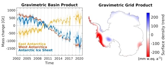
Figure 3 shows the mass change time series for AIS, Basin 06 and Basin 21 based on different variants of TSKs. Time series for all other basins (Figure 4b) are given in Figures S7–S11 in the SM. The AIS time series reveals changes on differing temporal scales. Beside seasonal variations, inter-annual changes, e.g., a less negative mass balance prior to 2008, become evident. Comparable changes are visible for Basin 21 (West Antarctica), whose mass balance is clearly negative throughout the entire observational period and is dominated by ice-dynamical mass losses. Basin 06 (East Antarctica) exhibits even more pronounced variations between the mass balance for different periods. Whereas no significant trend is observed between 2002 and 2009, the mass balance is clearly positive after 2009 and even for the period following two exceptional accumulation events in 2009 and 2011 [55]. A visual inspection of the time series shown in Figure 3 reveals differences between both the signal, e.g., the mass balance, and the noise level among the different variants, to be discussed in the following sections. The noise level also differs with time, e.g., a larger scatter is visible in the AIS time series in 2017, a period that suffered from the use of transplanted accelerometer data [25].
Noise Level
The noise level, assessed as described in Section 2.5.2, of the different variants of basin products is illustrated in Figure 4. It can be seen that considering the ANTOC pattern in the kernel design slightly reduces the noise level of the mass change time series. The largest overall reduction in the noise level between variant (ICE,FAR,0.1) and (ICE,FAR,ANTOC,0.1) is observed for AIS and is no larger than 1.1 Gt, while Basin 20 experienced the largest relative reduction (0.2 Gt, i.e., 2.3%). This indicates that there is only a low contamination risk by residual mass changes over the Antarctic Ocean. The level of noise reduction due to considering the ANTOC pattern differs between GRACE/GRACE-FO solution series and was found to be clearly larger for older data releases (e.g., RL05) exhibiting a larger noise level (e.g., [56]). Basin products of variant (ICE,FAR,ANTOC,1.0) have a clearly lower noise level than version (ICE,FAR,ANTOC,0.1), which was calculated using a weaker constraint on the mission error. The reduction in noise level, visible for all basins and aggregations except for Basin 08, is largest for Basin 06 (4.0 Gt) and can be as large as 32% of the absolute noise level (Basin 09). The lowest relative noise reduction is observed for the aggregations of EAIS, WAIS and AIS (below 2%), while the median over all basins is 16%.
An increased weight for the mission error constraint, i.e., a larger degree of smoothing, may lead to increased signal leakage. This is also revealed by the differing mass balance estimates and becomes even visible from the mass change time series shown in Figure 3. The mass loss inherent to the AIS time series decreases from 92.5 Gt a for variant (ICE,FAR,ANTOC,0.1) to 90.9 Gt a for version (ICE,FAR,ANTOC,1.0). Since signal leakage depends on the spatial pattern of the ongoing mass changes, both over the region of interest as well as in its surrounding, an increased mission error constraint does not necessarily lead to a reduced mass loss. For example, applying a stronger mission error constraint for Basin 21 increases the mass loss by 1.7 Gt a. These indications are supported by the leakage assessment.
Signal Leakage
Figure 5 indicates the differences between mass changes estimates derived by applying the various variants of TSKs to the synthetic data sets, and the synthetic truth of these data sets, to be used as a measure for the leakage errors induced by the TSKs (Section 2.2). Results for all other basins are shown in Figures S12–S16.
For AIS and Basin 06 largest signal leakage is caused by far-field mass signals such as from the global ocean (OCN) or continental hydrology (HYD), including their complementing oceanic component. As visible from Figure 5, TSKs which account for the ANTOC pattern are capable of significantly reducing the signal leakage stemming from OCN and HYD. This reduction is largest for the two data sets 18 and 19, which can be considered an upper limit for the approximated GAD uncertainty [18]. Basin 21, which has only a small ice-ocean-boundary and is smaller in size, is less sensitive to far-field signals and their oceanic complement. This is immediately revealed by the global view on the TSKs given in Figure S1. Signals of Antarctic surface mass balance and the mean annual mass balance cause the largest signal leakage for basins comparable to Basin 21 (Figures S12–S16).
In general, signal leakage strongly depends on the chosen ratio between the signal variances for clusters ICE and FAR. TSKs inferred with an increased ICE/FAR ratio will exhibit larger deviations from zero outside the ice-covered regions and hence, lead to increased leakage from signals outside the ice sheet, while leakage caused by AIS-signals is reduced. Reducing the ICE/FAR ratio will have the opposite effect. Hence, the ICE/FAR ratio needs to realize a trade-off between these two aspects of leakage. We found this trade-off best realized by the empirically derived ICE/FAR ratio of about 12 (Section 2.4).
To avoid a potential bias of the long-term changes in ice mass, a sound assessment of signal leakage associated with the pattern of the mean annual mass balance (i.e., the mass balance, AIS MB) is of particular importance. AIS MB leakage is largest for basins located in regions dominated by ice-dynamical changes (e.g., compare Basin 06 and 21). For the entire AIS, AIS MB leakage is below 1 Gt a and shows little variations among the different TSK-variants. This underlines that the TSKs are suitable to reliably reproduce the AIS mass balance. For Basin 21, considering the ANTOC pattern in the kernel design has a negligible effect, while the increased mission error constraint decreases the AIS MB leakage from 7.3 to 5.3 Gt a. Hence, the larger leakage-out caused by the smoother TSK of variant (ICE,FAR,ANTOC,1.0) is over-compensated by additional leakage-in. This finding is consistent with more negative mass balance estimate (1.7 Gt a) inferred from the basin product of the same variant compared to (ICE,FAR,ANTOC,0.1). Other synthetic data sets, e.g., AIS SMB for Basin 06 as well as Basin 21, indicate an amplified signal leakage caused by the smoother TSK. Although this does not apply for all regions (e.g., AIS) it is true for most basins and data sets as indicated by the RMS over all basins shown in Figure 5d.
TSK Selection
Based on the assessment of both the noise level of the basin products and the estimated signal leakage for all basins and aggregations we have selected the TSK-variant out of the three version under consideration most suitable for the final mass change product generation. It could be shown that considering the ANTOC pattern in the kernel design is important, particularly for the reduction of signal leakage stemming from the far-field. A larger mission error constraint, i.e., smoother TSKs lead to a clearly reduced noise level for most basins. This improvement is achieved at the cost of a potential increase of signal leakage. However, due to the dependencies of leakage errors on the spatial patterns of the ongoing mass changes, this increase in leakage is not consistently observed for all basins and synthetic data sets. Hence, we consider the noise reduction more valuable than a possibly small increase in signal leakage.
Therefore, we have chosen variant (ICE,FAR,ANTOC,1.0) for the final generation of our gravimetric mass change products. Figures showing TSKs for this variant and all basins are included in the SM, providing both a regional (Figures S2–S4) and a global view (Figures S5 and S6).
Mass Balance Estimates
The mass balance estimates, i.e., the linear trend derived by fitting the standard model to the basin product of the preferred variant (ICE,FAR,ANTOC,1.0), and the corresponding uncertainties are shown in Figure 6. Numbers for the different components of the uncertainty measures are provided in Table S1.
Over the entire GRACE/GRACE-FO period from 2002-04 through 2020-07, the AIS lost mass on an average rate of Gt a. Uncertainties account for the different components shown in Figure 6 (bars) and described in Section 2.5.4. This negative mass balance corresponds to an average contribution to global sea-level rise of mm a. Whereas AP and WAIS exhibit a negative mass balance of and Gt a, respectively, EAIS gained mass on an average rate of Gt a. The major contributions to WAIS mass loss arise from Basin 21 (Pine Island Glacier) and Basin 22 (Thwaites-Haynes-Pope-Smith-Kohler glacier complex), part of the Amundsen Sea Sector (ASS), with a mass balance of and Gt a, respectively. The only significantly positive mass balance in West Antarctica is evident for Basin 18 and coincides with the stagnating Kamb Ice Stream [57]. The positive mass balance of EAIS is dominated by the drainage basins of Dronning Maud Land (DML), in particular Basin 06 ( Gt a) and Basin 07 ( Gt a). Mass balance of Basin 06 was not entirely positive through the observational period. Whereas no mass balance different from zero was observed prior to 2009 ( Gt a), a pronounced mass gain between 2009 and 2011 ( Gt a) is followed by a smaller but still positive mass balance of Gt a after 2011 (note that the uncertainties given here are 1 formal errors of the fit).
Signal leakage is the dominating component of the overall mass balance uncertainty for single drainage basins located in West Antarctica (e.g., Basins 01, 20–24, 27) and can make up to 98.7% (Basin 22) of the total uncertainty (in terms of the variance, here and in the following). Another major contributor is the uncertainty of the GIA model correction, which strongly depends on the basin size and its location. In East Antarctica, where GIA models exhibit significant differences [58], their contribution can be as large as 93% (Basin 03). For larger basins or aggregations (e.g., Basin 17, EAIS, AIS) uncertainties in the trends of used auxiliary data sets like for SH degree or , which can make up to 25% and 17%, respectively, contribute significantly to the overall uncertainties. The AIS mass balance’s uncertainty is dominated by uncertainties in GIA ( Gt a, 56.2%), degree ( Gt a, 25.1%) and ( Gt a, 16.9%).
Velicogna et al. [59] found the AIS mass balance to be Gt a for the period 2002-04–2019-09. For the same period, we derived a mass balance estimate of Gt a. Both estimates were inferred from mass change time series based on CSR RL06 monthly solutions. Differences may be related to the applied GIA model correction. Although both studies make use of the IJ05_R2 model [28], an alternative GIA far-field component was applied by Velicogna et al. [59]. If GIA corrections would always be quantified, they could be compared across studies, but would of course still depend on the applied method, i.e., the sensitivity kernel. Our GIA corrections for all basins are given in Table S1. Loomis et al. [60] inferred a mass balance of Gt a for the period 2002-04–2019-08 from JPL RL06 SH solutions, which is clearly more negative than our estimate, although within the uncertainty ranges. The differing GRACE/GRACE-FO release adds an others degree of freedom to the search for the underlying reasons. Loomis et al. [60] indicate to apply the IJ05_R2 correction as well, again without providing an estimate for their correction. However, it is stated that their mass balance estimate would be 11 Gt a more negative when using ICE-6G_D instead. In contrast, when we switched from IJ05_R2 to ICE-6G_D our mass balance got 32 Gt a more negative, which is in better agreement with the differences between both models found by other studies [58]. Consequently, we are not able to finally prove that both mass balance estimates are at least comparable with respect to the applied model corrections. Besides differences in the input data, the approach applied for the mass change estimation can induce differences in the order of 10% of the AIS mass balance [18] and can only be quantified by means of a rigorous inter-comparison exercise as described by Groh et al. [18]. These aspects hamper a direct comparison of mass balances from literature or make it even impossible.
Inter-Comparison
We used mass change time series derived from independent observations for the inter-comparison with our GRACE/GRACE-FO-derived basin products (Figure 7). First, we used mass change time series derived from altimetry-observed surface elevation changes (SEC) [61] available for the period 1992–2018 and all basins constituting EAIS and WAIS. The temporal resolution of the SEC data set (140 d) is lower than for our product (monthly). Second, a monthly AIS time series from the input–output method (IOM) [59] covering 2002–2019 was used. For this purpose, we reverted the adjustments in trends applied by the authors to make the IOM data match their GRACE time series.
Figure 7a clearly reveals that IOM exhibits a larger loss in Antarctic ice mass than the gravimetric product, while the uncertainty ranges of both time series barely overlap. The revealed differences are confirmed by the corresponding mass balance estimates derived for the period where the gravimetric product is not affected by GRACE single accelerometer solutions, i.e., 2002-04–2016-08. The IOM mass balance ( Gt a) is more negative than the one derived from the gravimetric basin product ( Gt a), which agrees with the findings from the Ice Sheet Mass Balance Inter-comparison Exercise (IMBIE) [62]. Here, the uncertainty of the IOM mass balance was adopted from Rignot et al. [63] given for the period 1992–2017. It is noteworthy that the IOM data used in this study [59] are an update of Rignot et al. [63]. The mass balance derived from the IOM data of Velicogna et al. [59] is clearly less negative than those published by Rignot et al. [63] (cf. Gt a and Gt a, respectively, for the period 2009–2017).
To compare all three techniques, we also consider the aggregations of basins in DML (Basins 05–08, East Antarctica) and ASS (Basins 21–22, West Antarctica). For DML the overall trends in ice mass from SEC and IOM are in good agreement, while a larger mass gain is visible for the gravimetric product (Figure 7b). Between 2002 and 2009 distinct differences are visible among the three data sets. Whereas our product and SEC exhibit a mass gain, IOM suggests a decrease in ice mass. After 2015 all three time series reveal a comparable gain in mass. Moreover, the large mass gains caused by the two exceptional accumulation events in 2009 and 2011 are equally well reproduced by our product and IOM, but exhibit a significant smaller amplitude in the SEC record. For ASS, all time series show a significant mass loss, while the largest decrease is visible for IOM, followed by SEC and the gravimetric product (Figure 7). Disagreeing mass balance estimates from our product and SEC are primarily found for basins in DML (Basins 04–08) and entire EAIS. Here, uncertainties of GIA corrections and potential time-variable penetration of radar signals into the firn layer are limiting factors of GRACE/GRACE-FO- and SEC-derived mass balance estimates, respectively. Mass balance estimates for all regions are summarized in Table S2.
To check for a seamless continuation of the basin product within the GRACE-FO period and to rule out the presence of a potential offset between GRACE and GRACE-FO, we used the IOM and the SEC mass change time series. For this purpose, we assume that all three products just differ by a bias in the linear trend. Hence, we reduced the individual linear trends over the GRACE period not affected by single accelerometer gravity-field solutions (2002-04–2016-08) from each data set and compared the residuals with respect to this linear trend over the GRACE-FO period. From this comparison shown in Figure 7 (faint lines) we could not find an indication for a potential offset between the GRACE and GRACE-FO results in the gravimetric product. However, due to the uncertainties of the individual data sets and the varying discrepancies in the trend over different time periods, the SEC and IOM data do not provide a suitable reference for a rigorous assessment of the gravimetric product.
3.2.2. Gridded Products
The gridded mass change product can be considered the original product from which the basin products were derived by the summation of the kernels, or mass change estimates, for single grid cells. This allows for a flexible investigation of mass changes over arbitrarily defined regions of interest, such as e.g., the aggregations shown in Figure 7. The gridded product itself facilitates the investigation of the spatial patterns of mass changes signal, e.g., linear trends or seasonal amplitudes, over individual periods. As an example, Figure 8a depicts the spatial pattern of the linear trend over the entire study period (2002-04–2020–07) derived from the final product of variant (ICE,FAR,ANOTC,1.0). The pattern reveals the well-known pronounced mass losses along coastal WAIS, AP and in Basin 13 (Totten Glacier) as well as positive mass anomalies in DML and Basin 18 (Kamb Ice Stream). Figure 7a clearly reveals smaller changes in ice mass during the first six year of the observational period (2002-04–2007-12). The associated spatial pattern shown in Figure 8b depicts a less strong spread of the dynamic mass losses in WAIS. Moreover, negative mass balances are visible at the tip of AP and over a limited coastal region of Basin 13. For the period 2008-01–2020-07, Figure 8c reveals a pattern comparable to Figure 8a, but with increased amplitudes over WAIS, DML and Basin 13. When applying the TSKs with smaller mission error constraints, the patterns of the linear trends derived from the mass change products include artefacts of the north-south stripes (Figure S17).
Figure 8d shows the noise level of the final gridded product with an RMS over all grid cells of 86.7 mm w.eq. This RMS value is about half the RMS of the two variants of products derived with a weaker mission error constraint (173 mm w.eq.). The largest noise can be found along the coastal margins, stemming from residual oceanic mass changes as revealed by the analysis the synthetic data sets on a grid cell level [18]. However, compared to our products contributed to the round robin experiment of the CCI ice sheet projects [18], the noise level could be significantly decreased. This reduction goes back to an improved data quality of the up-to-date GRACE/GRACE-FO solutions as well as an adapted weighting of the cluster FAR, whose increased weight led to a reduction of leakage from near-coastal oceanic signals.
4. Conclusions and Outlook
We introduced an approach to directly tailor sensitivity kernels to be used in a regional integration approach for the generation of mass change products from GRACE/GRACE-FO time-variable gravity-field solutions. Our kernels minimize the sum of both propagated mission errors and leakage errors. TSKs are an intuitive tool for identifying potential signal leakage since they immediately provide insights in the weights applied to the data inside and outside the region of interest. They can be easily compared to kernels from different methods (e.g., a kernel derived by filtering and rescaling) and allow for an assessment of the individual methods. We did not just infer TSKs for ice sheet drainage basins and aggregations, but also for individual grid cells providing the basis for the gridded product. This product provides detailed insights in the spatial signatures of present-day ice mass changes. Moreover, it gives great flexibility to the users, since it allows the derivation of consistent basin products for any region of interest, e.g., the low accumulation zone in central East Antarctica or any basin aggregation not included in our basin product, just by combining the corresponding grid cells. The round robin experiment revealed the benefits of our methods and the competitiveness of the derived products [18].
Several enhancements of the proposed method are conceivable and subject of ongoing developments. We have demonstrated that by accounting for residual mass variations over the Antarctic Ocean (i.e., TSK variants including ANTOC), the noise level of the mass change products and signal leakage could be reduced. A further reduction would be possible be including additional information on sources of signal leakage. For example, the two largest ice shelves surrounding AIS, i.e., RIS and FRIS (Figure 4b), are not included in the ocean component of the AOD1B products (Section 2.4.2). Hence, by an additional parameterization of these two regions complementing the ANTOC pattern a further reduction of both the noise level and the signal leakage can be expected, in particular for adjacent regions. Considering additional spatial correlations of signals would allow a more realistic modelling of potential sources of leakage and increase consistency with the signal content of the L2 data. This may include the consideration of the ocean’s gravitational consistent response to the assumed signal variance for each point over land. Moreover, spatial correlations could be introduced by means of an autocorrelation function retrieved from geophysical models or by simply replacing the independent point masses used in the parametrization by spherical basis function with a suitable correlation length (e.g., a spherical Gaussian function or spherical splines) [64]. In this way, differing correlation lengths for signals in different compartments of the Earth system could be taken into account. Moreover, the used empirical error covariance model can be replaced by an actual error covariance model, if provided by the processing centers, to allow for a more realistic description of the mission errors. Finally, a future update of our mass change products will overcome the limitations of the spherical approximation used so far and will account for the Earth’s elliptical shape (e.g., [30,31]).
The gravimetric mass change products have been made available on an interactive data portal (data1.geo.tu-dresden.de/aisgmb, accessed on 7 March 2021), which provides convenient functionalities to browse, explore and download the data. The products receive regular, at least quarterly, updates, depending on the availability of new GRACE-FO L2 data. In particular, we provide the gridded product in different file formats (netcdf, geotiff, ascii) and the basin product (ascii format) for 26 drainage basins and the aggregations of AP, EAIS, WAIS and AIS including the noise level for each region. The mass balance estimates for all basins and aggregations, their overall uncertainties, the applied GIA corrections as well as the corresponding changes in mean sea level are provided as an additional product (ascii format). All basin-related time series and estimates are also available in a single netcdf file. TSKs can be provided upon request.
Supplementary Materials
The following are available online at https://0-www-mdpi-com.brum.beds.ac.uk/article/10.3390/rs13091736/s1, Figure S1: Global view on different variants of TSKs, Figures S2–S4: Preferred variant of TSKs for all regions, Figures S5–S6: Global view on preferred variant of TSKs for all regions, Figures S7–S11: basin products for all regions, Figures S12–S16: Results from synthetic data sets for all regions, Table S1: Mass balance estimates and uncertainties, Table S2: Mass balance estimates GRACE/GRACE-FO, SEC, IOM, Figure S17: Linear trends and noise levels for gridded products.
Author Contributions
Conceptualization, A.G. and M.H.; data curation, A.G.; methodology, A.G. and M.H.; software, A.G. and M.H.; formal analysis, A.G.; investigation, A.G.; writing—original draft preparation, A.G.; writing—review & editing, M.H.; visualization, A.G.; supervision, M.H. Both authors have read and agreed to the published version of the manuscript.
Funding
This study was supported by the European Space Agency through the Climate Change Initiative (CCI) projects Antarctic Ice Sheet CCI+ (contract number 4000126813/19/I-NB), Greenland Ice Sheet CCI+ (contract number 4000126523/19/I-NB) and Sea-level Budget Closure CCI (contract number 4000119910/17/I-NB). We acknowledge support by the Open Access Publication Funds of the SLUB/TU Dresden.
Data Availability Statement
The mass change products presented in this study are openly available in the data portal at data1.geo.tu-dresden.de/aisgmb (accessed on 7 March 2021). The tailored sensitivity kernels are available on request from the corresponding author.
Acknowledgments
We thank the German Space Operations Center (GSOC) of the German Aerospace Center (DLR) for providing continuously and nearly 100% of the raw telemetry data of the twin GRACE satellites.
Conflicts of Interest
The authors declare no conflict of interest. The funders had no role in the design of the study; in the collection, analyses, or interpretation of data; in the writing of the manuscript, or in the decision to publish the results.
References
- Tapley, B.; Bettadpur, S.; Ries, J.; Thompson, P.; Watkins, M. GRACE Measurements of Mass Variability in the Earth System. Science 2004, 305, 503–505. [Google Scholar] [CrossRef] [PubMed] [Green Version]
- Tapley, B.; Watkins, M.; Flechtner, F.; Reigber, C.; Bettadpur, S.; Rodell, M.; Sasgen, I.; Famiglietti, J.; Landerer, F.; Chambers, D.; et al. Contributions of GRACE to understanding climate change. Nat. Clim. Chang. 2019, 9, 358–369. [Google Scholar] [CrossRef] [PubMed]
- Landerer, F.; Flechtner, F.; Save, H.; Webb, F.; Bandikova, T.; Bertiger, W.; Bettadpur, S.; Byun, S.; Dahle, C.; Dobslaw, H.; et al. Extending the global mass change data record: GRACE Follow-On instrument and science data performance. Geophys. Res. Lett. 2020, 47, e2020GL088306. [Google Scholar] [CrossRef]
- Swenson, S.; Wahr, J. Methods for inferring regional surface-mass anomalies from Gravity Recovery and Climate Experiment (GRACE) measurements of time-variable gravity. J. Geophys. Res. 2002, 107, 2193. [Google Scholar] [CrossRef] [Green Version]
- Baur, O.; Kuhn, M.; Featherstone, W. GRACE-derived ice-mass variations over Greenland by accounting for leakage effects. J. Geophys. Res. 2009, 114, B06407. [Google Scholar] [CrossRef] [Green Version]
- Velicogna, I.; Wahr, J. Greenland mass balance from GRACE. Geophys. Res. Lett. 2005, 32, L18505. [Google Scholar] [CrossRef] [Green Version]
- Horwath, M.; Dietrich, R. Signal and error in mass change inferences from GRACE: The case of Antarctica. Geophys. J. Int. 2009, 177, 849–864. [Google Scholar] [CrossRef] [Green Version]
- Jacob, T.; Wahr, J.; Pfeffer, W.; Swenson, S. Recent contributions of glaciers and ice caps to sea level rise. Nature 2012, 482, 514–518. [Google Scholar] [CrossRef]
- Wouters, B.; Chambers, D.; Schrama, E. GRACE observes small-scale mass loss in Greenland. Geophys. Res. Lett. 2008, 35, L20501. [Google Scholar] [CrossRef] [Green Version]
- Schrama, E.; Wouters, B.; Rietbroek, R. A mascon approach to assess ice sheet and glacier mass balances and their uncertainties from GRACE data. J. Geophys. Res. Solid Earth 2014, 119, 6048–6066. [Google Scholar] [CrossRef]
- Forsberg, R.; Sørensen, L.; Simonsen, S. Greenland and Antarctica Ice Sheet Mass Changes and Effects on Global Sea Level. Surv. Geophys. 2017, 38, 89–104. [Google Scholar] [CrossRef] [Green Version]
- Ran, J.; Ditmar, P.; Klees, R.; Farahani, H. Statistically optimal estimation of Greenland Ice Sheet mass variations from GRACE monthly solutions using an improved mascon approach. J. Geod. 2018, 92, 299–319. [Google Scholar] [CrossRef] [PubMed] [Green Version]
- Swenson, S.; Wahr, J. Post-processing removal of correlated errors in GRACE data. Geophys. Res. Lett. 2006, 33, L08402. [Google Scholar] [CrossRef]
- Kusche, J. Approximate decorrelation and non-isotropic smoothing of time-variable GRACE-type gravity field models. J. Geod. 2007, 81, 733–749. [Google Scholar] [CrossRef] [Green Version]
- Landerer, F.; Swenson, S. Accuracy of scaled GRACE terrestrial water storage estimates. Water Resour. Res. 2012, 48. [Google Scholar] [CrossRef]
- Vishwakarma, B.; Horwath, M.; Devaraju, B.; Groh, A.; Sneeuw, N. A Data-Driven Approach for Repairing the Hydrological Catchment Signal Damage Due to Filtering of GRACE Products. Water Resour. Res. 2017, 53, 9824–9844. [Google Scholar] [CrossRef]
- Barletta, V.; Sørensen, L.; Forsberg, R. Scatter of mass changes estimates at basin scale for Greenland and Antarctica. Cryosphere 2013, 7, 1411–1432. [Google Scholar] [CrossRef] [Green Version]
- Groh, A.; Horwath, M.; Horvath, A.; Meister, R.; Sørensen, L.; Barletta, V.; Forsberg, R.; Wouters, B.; Ditmar, P.; Ran, J.; et al. Evaluating GRACE Mass Change Time Series for the Antarctic and Greenland Ice Sheet—Methods and Results. Geosciences 2019, 9, 415. [Google Scholar] [CrossRef] [Green Version]
- Bettadpur, S. UTCSR Level-2 Processing Standards Document for Level-2 Product Release 0006, v5.0; Technical Report; Center for Space Research, The University of Texas at Austin: Austin, TX, USA, 2018. [Google Scholar]
- Save, H. CSR Level-2 Processing Standards Document for Level-2 Product Release 06, v1.1. Technical Report; Center for Space Research, The University of Texas at Austin: Austin, TX, USA, 2019. [Google Scholar]
- Swenson, S.; Chambers, D.; Wahr, J. Estimating geocenter variations from a combination of GRACE and ocean model output. J. Geophys. Res. 2008, B113, B08410. [Google Scholar] [CrossRef] [Green Version]
- Bergmann-Wolf, I.; Zhang, L.; Dobslaw, H. Global Eustatic Sea-Level Variations for the Approximation of Geocenter Motion from Grace. J. Geod. Sci. 2014, 4. [Google Scholar] [CrossRef]
- Sun, Y.; Riva, R.; Ditmar, P. Optimizing estimates of annual variations and trends in geocenter motion and J2 from a combination of GRACE data and geophysical models. J. Geophys. Res. Solid Earth 2016, 121, 8352–8370. [Google Scholar] [CrossRef] [Green Version]
- Loomis, B.; Rachlin, K.; Luthcke, S. Improved Earth oblateness rate reveals increased ice sheet losses and mass-driven sea level rise. Geophys. Res. Lett. 2019, 46, 6910–6917. [Google Scholar] [CrossRef]
- Loomis, B.; Rachlin, K.; Wiese, D.; Landerer, F.; Luthcke, S. Replacing GRACE/GRACE-FO C30 with satellite laser ranging: Impacts on Antarctic Ice Sheet mass change. Geophys. Res. Lett. 2020. [Google Scholar] [CrossRef]
- Landerer, F.; Flechtner, F.; Save, H.; Dahle, C.; Watkins, M. GRACE Follow-on Science Data System Newsletter Report: June/July 2020 (No. 14). 2020. Available online: ftp://isdcftp.gfz-potsdam.de/grace-fo/DOCUMENTS/NEWSLETTER/2020/GRACE-FO_SDS_NL_014_202006.pdf (accessed on 7 March 2021).
- Bruinsma, S.; Lemoine, J.M.; Biancale, R.; Valès, N. CNES/GRGS 10-day gravity field models (release 2) and their evaluation. Adv. Space Res. 2010, 45, 587–601. [Google Scholar] [CrossRef]
- Ivins, E.; James, T.; Wahr, J.; Schrama, E.; Landerer, F.; Simon, K. Antarctic contribution to sea level rise observed by GRACE with improved GIA correction. J. Geophys. Res. Solid Earth 2013, 118, 3126–3141. [Google Scholar] [CrossRef] [Green Version]
- Farrell, W. Deformation of the Earth by Surface Loads. Rev. Geophys. Space Phys. 1972, 10, 761–797. [Google Scholar] [CrossRef]
- Ditmar, P. Conversion of time-varying Stokes coefficients into mass anomalies at the Earth’s surface considering the Earth’s oblateness. J. Geod. 2018, 92, 1401–1412. [Google Scholar] [CrossRef] [Green Version]
- Ghobadi-Far, K.; Šprlák, M.; Han, S.C. Determination of ellipsoidal surface mass change from GRACE time-variable gravity data. Geophys. J. Int. 2019, 219, 248–259. [Google Scholar] [CrossRef]
- Van Wessem, J.; Reijmer, C.; Morlighem, M.; Mouginot, J.; Rignot, E.; Medley, B.; Joughin, I.; Wouters, B.; Depoorter, M.; Bamber, J.; et al. Improved representation of East Antarctic surface mass balance in a regional atmospheric climate model. J. Glaciol. 2014, 60, 761–770. [Google Scholar] [CrossRef] [Green Version]
- Noël, B.; van de Berg, W.; van Meijgaard, E.; Kuipers Munneke, P.; van de Wal, R.; van den Broeke, M. Evaluation of the updated regional climate model RACMO2.3: Summer snowfall impact on the Greenland Ice Sheet. Cryosphere 2015, 9, 1831–1844. [Google Scholar] [CrossRef] [Green Version]
- McMillan, M.; Shepherd, A.; Sundal, A.; Briggs, K.; Muir, A.; Ridout, A.; Hogg, A.; Wingham, D. Increased ice losses from Antarctica detected by CryoSat-2. Geophys. Res. Lett. 2014, 41, 3899–3905. [Google Scholar] [CrossRef]
- Groh, A.; Ewert, H.; Rosenau, R.; Fagiolini, E.; Gruber, C.; Floricioiu, D.; Abdel Jaber, W.; Linow, S.; Flechtner, F.; Eineder, M.; et al. Mass, volume and velocity of the Antarctic Ice Sheet: Present-day changes and error effects. Surv. Geophys. 2014, 35, 1481–1505. [Google Scholar] [CrossRef] [Green Version]
- Gardner, A.; Moholdt, G.; Wouters, B.; Wolken, G.; Burgess, D.; Sharp, M.; Cogley, J.; Braun, C.; Labine, C. Sharply increased mass loss from glaciers and ice caps in the Canadian Arctic Archipelago. Nature 2011, 473, 357–360. [Google Scholar] [CrossRef] [PubMed]
- Flechtner, F. AOD1B Product Description Document for Product Releases 01 to 04; Technical Report; Deutsches GeoForschungsZentrum GFZ: Potsdam, Germany, 2007. [Google Scholar]
- Flechtner, F.; Dobslaw, H.; Fagiolini, E. AOD1B Product Description Document for Product Release 05, Rev. 4.3; Technical Report; Deutsches GeoForschungsZentrum GFZ: Potsdam, Germany, 2015. [Google Scholar]
- Döll, P.; Kaspar, F.; Lehner, B. A global hydrological model for deriving water availability indicators: Model tuning and validation. J. Hydrol. 2003, 270, 105–134. [Google Scholar] [CrossRef]
- Dobslaw, H.; Bergmann-Wolf, I.; Dill, R.; Poropat, L.; Thomas, M.; Dahle, C.; Esselborn, S.; König, R.; Flechtner, F. A new high-resolution model of non-tidal atmosphere and ocean mass variability for de-aliasing of satellite gravity observations: AOD1B RL06. Geophys. J. Int. 2017, 211, 263–269. [Google Scholar] [CrossRef] [Green Version]
- Preisendorfer, R. Principal Component Analysis in Meteorology and Oceanography; Elsevier Science Publishers B.V.: Amsterdam, The Netherlands, 1988. [Google Scholar]
- Bergmann, I.; Dobslaw, H. Short-term transport variability of the Antarctic Circumpolar Current from satellite gravity observations. J. Geophys. Res. Ocean. 2012, 117, C05044. [Google Scholar] [CrossRef] [Green Version]
- Zwally, H.; Giovinetto, M.; Beckley, M.; Saba, J. Antarctic and Greenland Drainage Systems. 2012. Available online: http://icesat4.gsfc.nasa.gov/cryo_data/ant_grn_drainage_systems.php (accessed on 7 March 2021).
- Ray, R.; Luthcke, S. Tide model errors and GRACE gravimetry: Towards a more realistic assessment. Geophys. J. Int. 2006, 167, 1055–1059. [Google Scholar] [CrossRef] [Green Version]
- Whitehouse, P.; Bentley, M.; Milne, G.; King, M.; Thomas, I. A new glacial isostatic adjustment model for Antarctica: Calibrated and tested using observations of relative sea-level change and present-day uplift rates. Geophys. J. Int. 2012, 190, 1464–1482. [Google Scholar] [CrossRef] [Green Version]
- Peltier, W.; Argus, D.; Drummond, R. Comment on “An Assessment of the ICE-6G_C (VM5a) Glacial Isostatic Adjustment Model” by Purcell et al. J. Geophys. Res. Solid Earth 2018, 123, 2019–2028. [Google Scholar] [CrossRef]
- Caron, L.; Ivins, E.; Larour, E.; Adhikari, S.; Nilsson, J.; Blewitt, G. GIA Model Statistics for GRACE Hydrology, Cryosphere, and Ocean Science. Geophys. Res. Lett. 2018, 45. [Google Scholar] [CrossRef]
- Cheng, M.; Ries, J.; Tapley, B. Geocenter Variations from Analysis of SLR Data. In Reference Frames for Applications in Geosciences; International Association of Geodesy Symposia; Altamimi, Z., Collilieux, X., Eds.; Springer: Berlin/Heidelberg, Germany, 2013; Volume 138, pp. 19–25. [Google Scholar] [CrossRef]
- Rietbroek, R.; Fritsche, M.; Brunnabend, S.E.; Daras, I.; Kusche, J.; Schröter, J.; Flechtner, F.; Dietrich, R. Global surface mass from a new combination of GRACE, modelled OBP and reprocessed GPS data. J. Geodyn. 2012, 59–60, 64–71. [Google Scholar] [CrossRef]
- A, G.; Wahr, J.; Zhong, S. Computations of the viscoelastic response of a 3-D compressible Earth to surface loading: An application to Glacial Isostatic Adjustment in Antarctica and Canada. Geophys. J. Int. 2013, 192, 557–572. [Google Scholar] [CrossRef]
- Cheng, M.; Tapley, B.; Ries, J. Deceleration in the Earth’s oblateness. J. Geophys. Res. Solid Earth 2013, 118, 740–747. [Google Scholar] [CrossRef]
- Bloßfeld, M.; Müller, H.; Gerstl, M.; Štefka, V.; Bouman, J.; Göttl, F.; Horwath, M. Second-degree Stokes coefficients from multi-satellite SLR. J. Geod. 2015, 89, 857–871. [Google Scholar] [CrossRef]
- Cheng, M.; Ries, J. Decadal variation in Earth’s oblateness (J2) from satellite laser ranging data. Geophys. J. Int. 2017, 212, 1218–1224. [Google Scholar] [CrossRef]
- König, R.; Schreiner, P.; Dahle, C. Monthly estimates of C(2,0) generated by GFZ from SLR satellites based on GFZ GRACE/GRACE-FO RL06 background models. V. 1.0. GFZ Data Services 2019. [Google Scholar] [CrossRef]
- Lenaerts, J.; van Meijgaard, E.; van den Broeke, M.; Ligtenberg, S.; Horwath, M.; Isaksson, E. Recent snowfall anomalies in Dronning Maud Land, East Antarctica, in a historical and future climate perspective. Geophys. Res. Lett. 2013, 40, 2684–2688. [Google Scholar] [CrossRef]
- Dahle, C.; Murböck, M.; Flechtner, F.; Dobslaw, H.; Michalak, G.; Neumayer, K.; Abrykosov, O.; Reinhold, A.; König, R.; Sulzbach, R.; et al. The GFZ GRACE RL06 Monthly Gravity Field Time Series: Processing Details and Quality Assessment. Remote Sens. 2019, 11, 2116. [Google Scholar] [CrossRef] [Green Version]
- Pritchard, H.; Arthern, R.; Vaughan, D.; Edwards, L. Extensive dynamic thinning on the margins of the Greenland and Antarctic ice sheets. Nature 2009, 461, 971–975. [Google Scholar] [CrossRef]
- Martín-Español, A.; King, M.; Zammit-Mangion, A.; Andrews, S.; Moore, P.; Bamber, J. An assessment of forward and inverse GIA solutions for Antarctica. J. Geophys. Res. Solid Earth 2016, 121, 6947–6965. [Google Scholar] [CrossRef] [Green Version]
- Velicogna, I.; Mohajerani, Y.; Landerer, F.; Mouginot, J.; Noel, B.; Rignot, E.; Sutterley, T.; van den Broeke, M.; van Wessem, J.; Wiese, D. Continuity of ice sheet mass loss in Greenland and Antarctica from the GRACE and GRACE Follow-On missions. Geophys. Res. Lett. 2020, 47, e2020GL087291. [Google Scholar] [CrossRef] [Green Version]
- Loomis, B.; Luthcke, S.; Sabaka, T. Regularization and error characterization of GRACE mascons. J. Geod. 2019. [Google Scholar] [CrossRef] [PubMed]
- Shepherd, A.; Gilbert, L.; Muir, A.; Konrad, H.; McMillan, M.; Slater, T.; Briggs, K.; Sundal, A.; Hogg, A.; Engdahl, M. Trends in Antarctic Ice Sheet Elevation and Mass. Geophys. Res. Lett. 2019. [Google Scholar] [CrossRef] [Green Version]
- The IMBIE Team. Mass balance of the Antarctic Ice Sheet from 1992 to 2017. Nature 2018, 558, 219–222. [Google Scholar] [CrossRef] [PubMed] [Green Version]
- Rignot, E.; Mouginot, J.; Scheuchl, B.; van den Broeke, M.; Van Wessem, J.; Morlighem, M. Four decades of Antarctic Ice Sheet mass balance from 1979–2017. Proc. Natl. Acad. Sci. USA 2019, 116, 1095–1103. [Google Scholar] [CrossRef] [PubMed] [Green Version]
- Baxter, B.; Hubbert, S. Radial Basis Functions for the Sphere. In Recent Progress in Multivariate Approximation; Haussmann, W., Jetter, K., Reimer, M., Eds.; Birkhäuser: Basel, Switzerland, 2001; pp. 33–47. [Google Scholar] [CrossRef] [Green Version]
Figure 1.
Residual surface density anomalies with respect to the standard model derived from filtered CSR RL06 monthly solutions (corrected for cumulative surface mass balance anomalies over the Antarctic Ice Sheet): (a) standard deviation and (b) first empirical orthogonal function (EOF) from a principal component analysis of the residuals over the adjacent ocean. The spatial pattern in (b) is scaled by the standard deviation of the corresponding principal component.

Figure 2.
Different realizations (columns) of tailored sensitivity kernels (unitless) for integrating mass changes of (a–c) the Antarctic Ice Sheet, (d–f) Basin 06, (g–i) Basin 21 and (j–l) a grid cell marked by the red cross. Contour lines (thin) are given at intervals of 0.1 and 0.005 for panels (a–i) and (j–l), respectively. Thick contours lines are shown for multiples of 0.5. Red lines depict the basin outlines. Faint blue dots in panel (j) indicate the locations of additional points from the cluster ICE. Please note the differing color scales for panels (a–i) and (j–l).

Figure 3.
Mass change time series, i.e., the gravimetric basin product, for (a) the entire Antarctic Ice Sheet, (b) Basin 06 and (c) Basin 21 derived using different realizations of tailored sensitivity kernels.
Figure 3.
Mass change time series, i.e., the gravimetric basin product, for (a) the entire Antarctic Ice Sheet, (b) Basin 06 and (c) Basin 21 derived using different realizations of tailored sensitivity kernels.

Figure 4.
(a) Root mean square of the noise in gravimetric basin products for individual drainage basins and aggregations. Colored symbols indicate different realizations of tailored sensitivity kernels used to derive the basin products. Grey bars show the ratio between the basin area and the area of the entire AIS (linear scale at the right-hand side ordinate axis). (b) Overview of Antarctic drainage basins and aggregations (grey shades) based on the basin definitions by Zwally et al. [43]. FRIS and RIS indicate the location of the Filchner-Ronne Ice Shelf and the Ross Ice Shelf, respectively.

Figure 5.
Differences between mass change estimates derived from synthetic data sets (Table 1) and the their corresponding true mass changes for (a) the entire Antarctic Ice Sheet, (b) Basin 06, (c) Basin 21 derived using different realizations of tailored sensitivity kernels and (d) the root mean square (RMS) over all basins and aggregations (Figure 4b).

Figure 6.
Components (bars) contributing to the overall uncertainty of the mass balance (numbers) for the final mass change basin products of variant (ICE,FAR,ANTOC,1.0). The overall uncertainty accounts for formal errors from the least-squares adjustment, for uncertainties of the degree addition, related to the replacement, of the glacial isostatic adjustment (GIA) model correction and for leakage errors. Bars indicate the components’ share of the total variance.

Figure 7.
Mass change time series from GRACE/GRACE-FO using tailored sensitivity kernels of variant (ICE,FAR,ANTOC,1.0), from satellite altimetry-derived surface elevation changes (SEC, [61]) and from the input–output-method (IOM, [59]) for (a) the entire Antarctic Ice Sheet (AIS), (b) Dronning Maud Land (i.e., Basins 05–08) and (c) Amundsen Sea Sector (i.e., Basins 21–22). Faint lines indicate the corresponding residuals with respect to the linear trend over the period from 2002-04 through 2016-08.

Figure 8.
(a–c) Linear trends over different periods derived from the gridded mass change product using the standard model. (d) Noise level of each grid cell, assessed as described in Section 2.5.2. All results are based on variant (ICE,FAR,ANTOC,1.0) of the gridded product.
Figure 8.
(a–c) Linear trends over different periods derived from the gridded mass change product using the standard model. (d) Noise level of each grid cell, assessed as described in Section 2.5.2. All results are based on variant (ICE,FAR,ANTOC,1.0) of the gridded product.


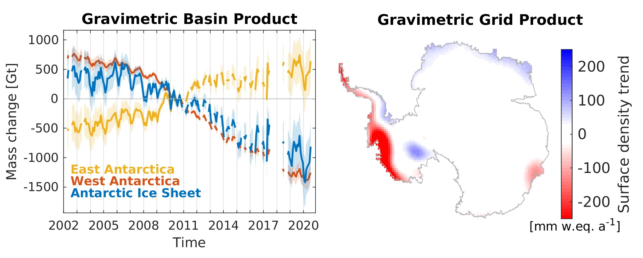
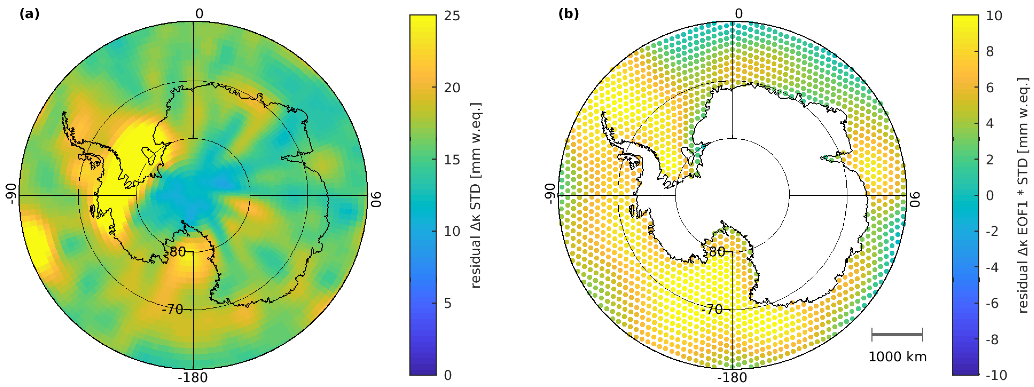
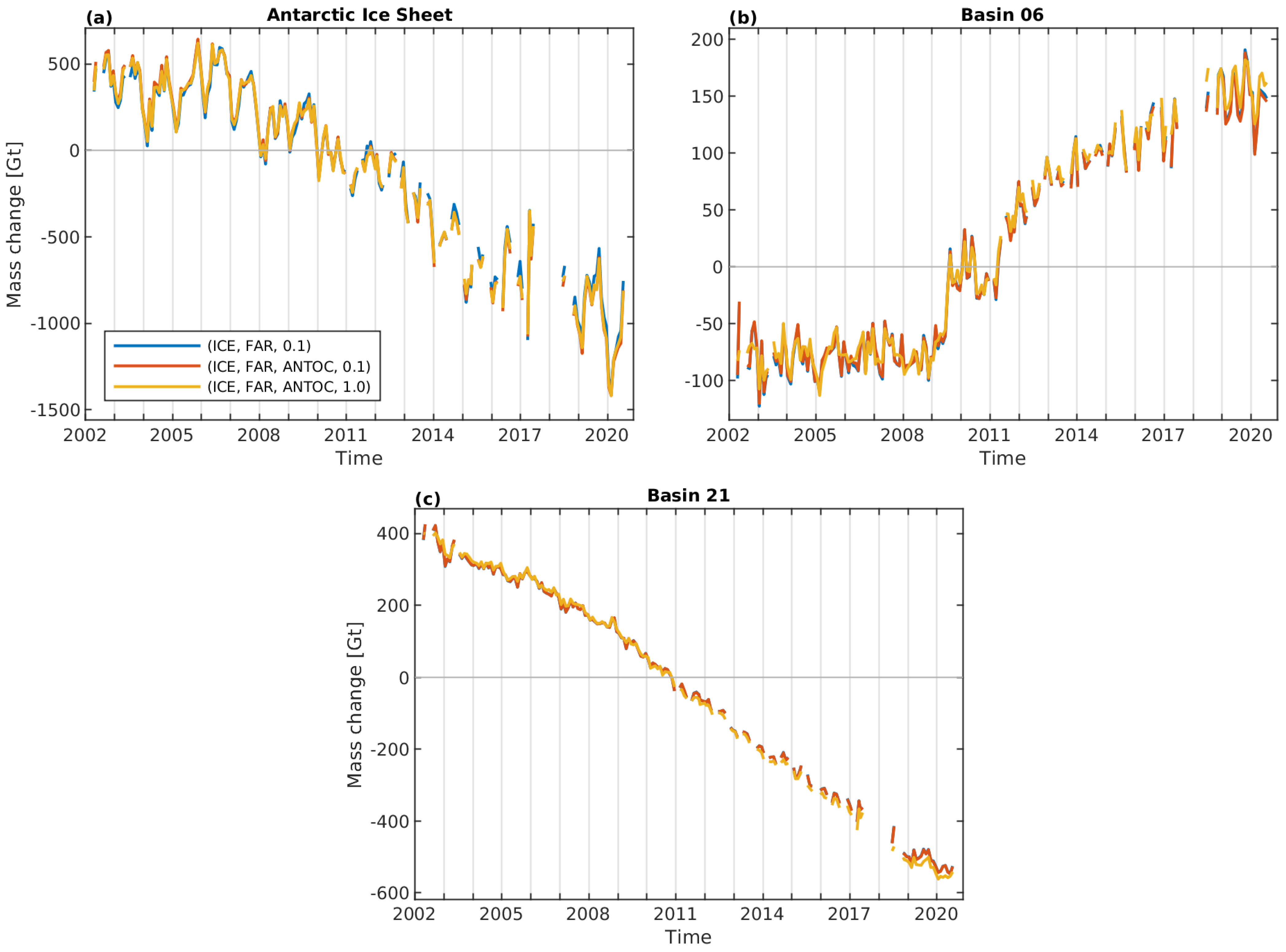
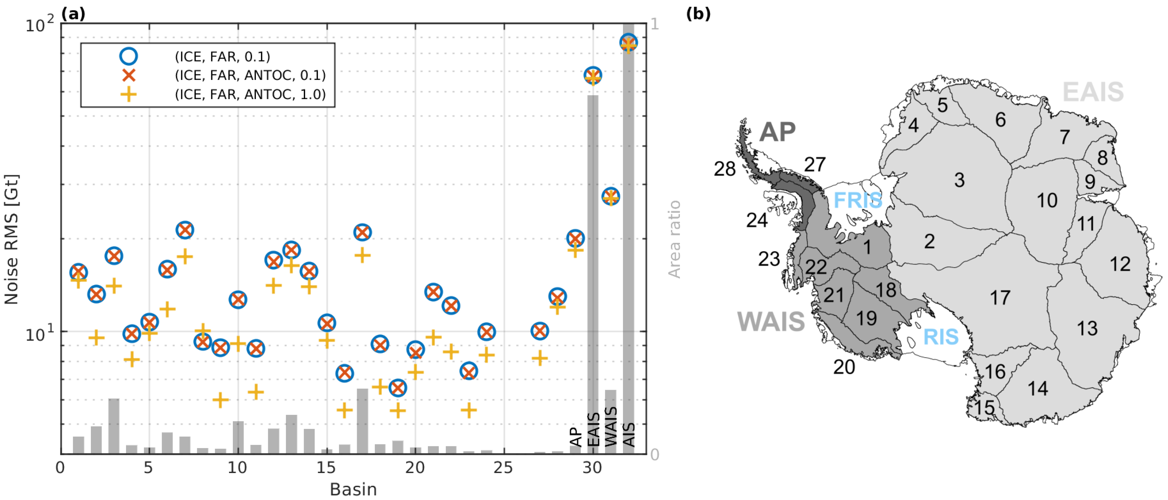
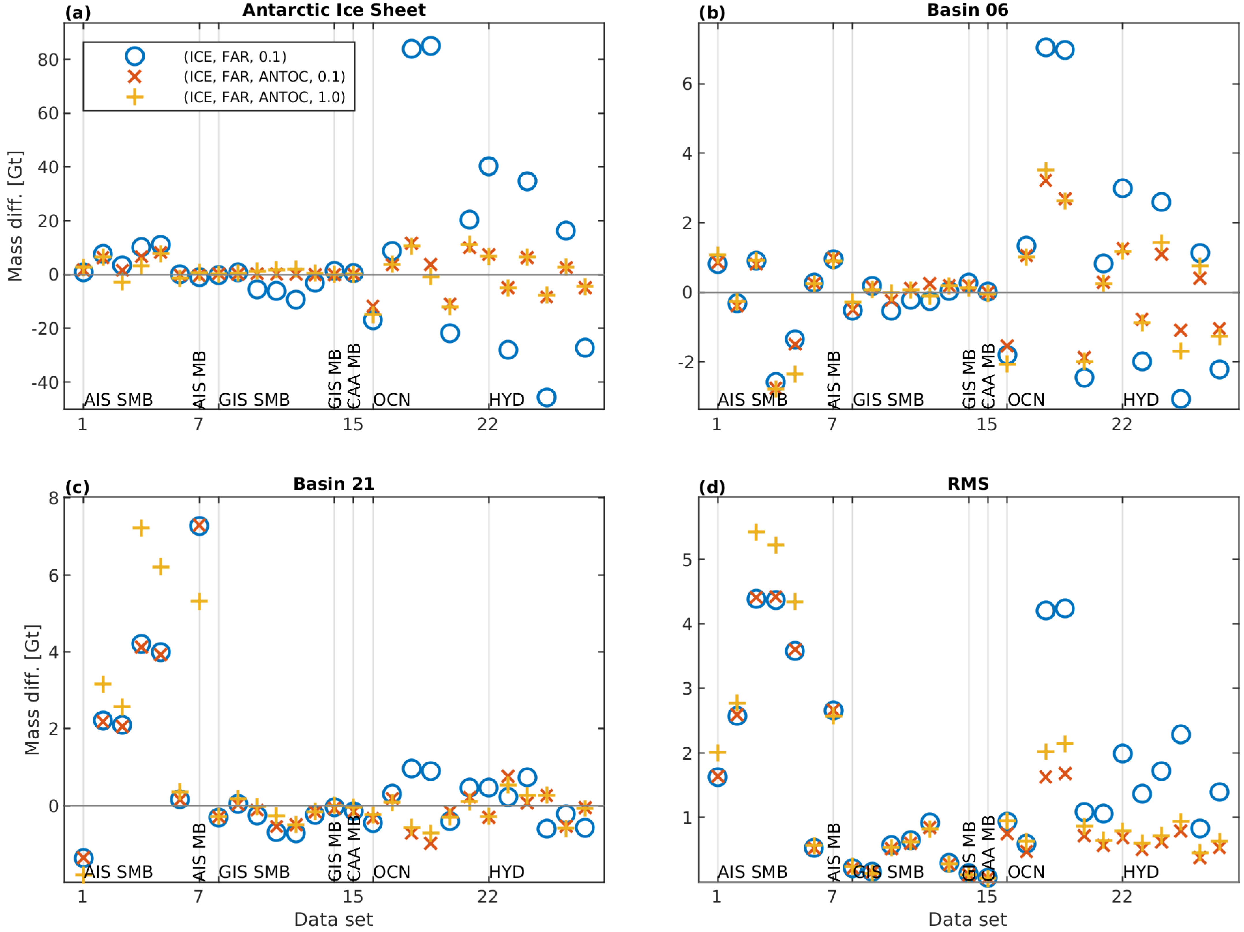
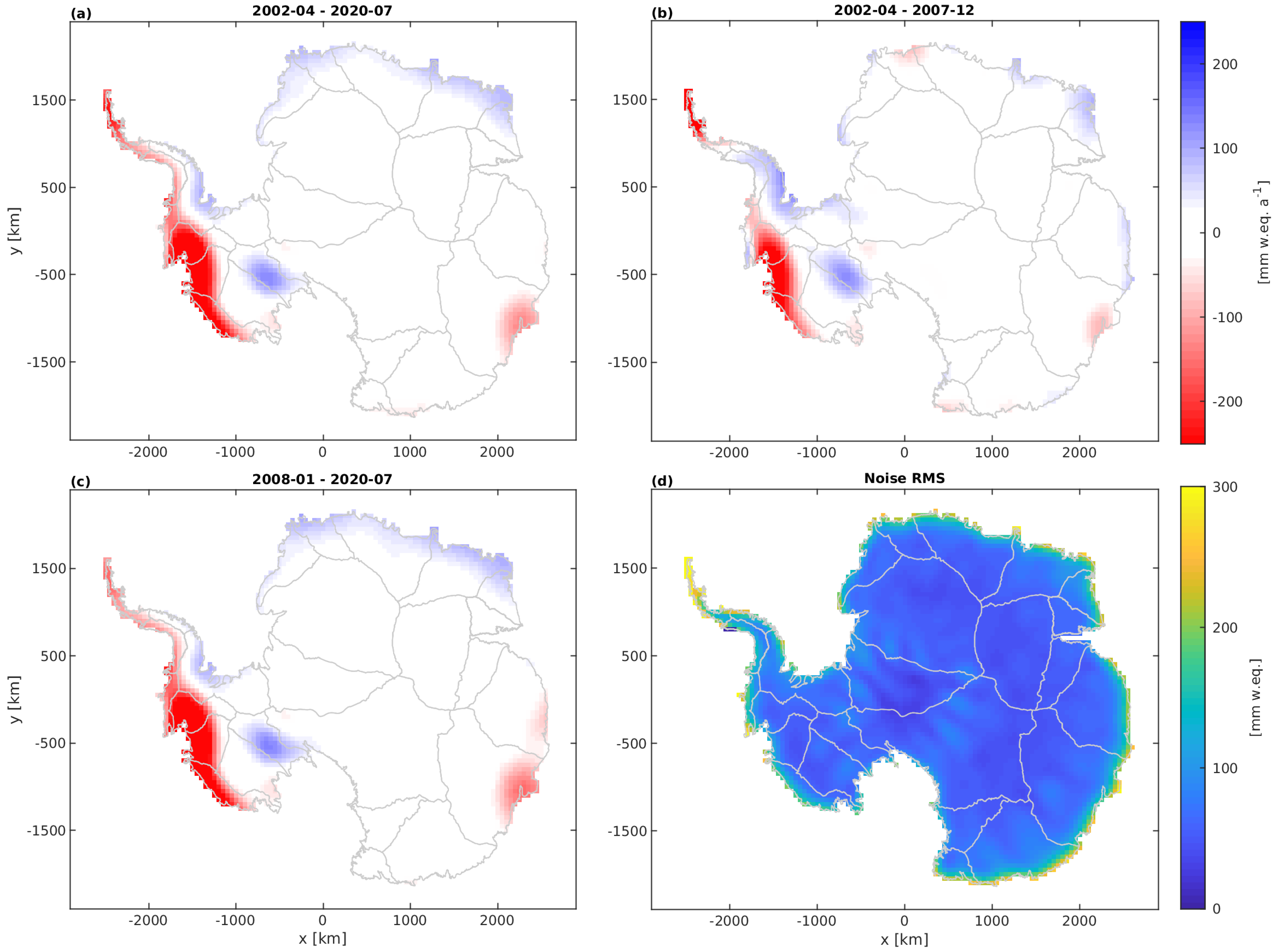
Table 1.
Synthetic data sets used to assess signal leakage. Dates indicate the epochs selected from perennial model time series.
Table 1.
Synthetic data sets used to assess signal leakage. Dates indicate the epochs selected from perennial model time series.
| ID | Acronym | Description |
|---|---|---|
| 01–06 | AIS SMB | Six data sets of modelled spatial variability in Antarctic surface mass balance |
| Epochs: 1980-01, 1986-10, 1996-01, 2004-08, 2009-02, 2014-08 | ||
| 07 | AIS MB | Spatial pattern of the mean annual AIS mass change as observed by satellite altimetry |
| 08–13 | GIS SMB | Six data sets of modelled spatial variability in Greenland surface mass balance |
| Epochs: 1960-05, 1970-10, 1980-05, 1990-10, 2000-05, 2010-10 | ||
| 14 | GIS MB | Spatial pattern of the mean annual GIS mass change as observed by satellite altimetry |
| 15 | CAA MB | Spatially uniform mean annual ice mass change over the Canadian Arctic Archipelago |
| 16–21 | OCN | Six data sets simulating residual global oceanic mass variations (e.g., due to errors in the GRACE de-aliasing products) |
| Epochs: 2002-09, 2005-03, 2006-09, 2009-03, 2010-09, 2013-03 | ||
| 22–27 | HYD | Six data sets of modelled mass changes in global continental hydrology (excluding AIS and GIS) |
| Epochs: 2004-03, 2005-09, 2007-01, 2009-01, 2010-12, 2011-10 |
Table 2.
Overview of parametrizations, i.e., spatial coverage of the different clusters of points, grid type, grid cell area and assumed signal variance, used to derive tailored sensitivity kernels .
Table 2.
Overview of parametrizations, i.e., spatial coverage of the different clusters of points, grid type, grid cell area and assumed signal variance, used to derive tailored sensitivity kernels .
| Cluster | Coverage | Grid/Cell Area | Signal Variance |
|---|---|---|---|
| ICE | Grid cells covering the AIS | polar-stereo. () | (400 mm w.eq.) |
| FAR | Far-field grid cells outside the AIS | icosahedron () | (33.6 mm w.eq.) |
| ANTOC | Spatial pattern covering the Antarctic Ocean () | icosahedron () | Spatially variable, median: (14.7 mm w.eq.) |
Publisher’s Note: MDPI stays neutral with regard to jurisdictional claims in published maps and institutional affiliations. |
© 2021 by the authors. Licensee MDPI, Basel, Switzerland. This article is an open access article distributed under the terms and conditions of the Creative Commons Attribution (CC BY) license (https://creativecommons.org/licenses/by/4.0/).
Share and Cite
MDPI and ACS Style
Groh, A.; Horwath, M. Antarctic Ice Mass Change Products from GRACE/GRACE-FO Using Tailored Sensitivity Kernels. Remote Sens. 2021, 13, 1736. https://0-doi-org.brum.beds.ac.uk/10.3390/rs13091736
AMA Style
Groh A, Horwath M. Antarctic Ice Mass Change Products from GRACE/GRACE-FO Using Tailored Sensitivity Kernels. Remote Sensing. 2021; 13(9):1736. https://0-doi-org.brum.beds.ac.uk/10.3390/rs13091736
Chicago/Turabian StyleGroh, Andreas, and Martin Horwath. 2021. "Antarctic Ice Mass Change Products from GRACE/GRACE-FO Using Tailored Sensitivity Kernels" Remote Sensing 13, no. 9: 1736. https://0-doi-org.brum.beds.ac.uk/10.3390/rs13091736
Note that from the first issue of 2016, this journal uses article numbers instead of page numbers. See further details here.