
Comparison of Target Detectors to Identify Icebergs in Quad-Polarimetric L-Band Synthetic Aperture Radar Data


Department of Biological and Environmental Sciences, Faculty of Natural Sciences, University of Stirling, Stirling FK9 4LA, UK
*
Author to whom correspondence should be addressed.
Remote Sens. 2021, 13(9), 1753; https://0-doi-org.brum.beds.ac.uk/10.3390/rs13091753
Submission received: 12 March 2021
/
Revised: 28 April 2021
/
Accepted: 29 April 2021
/
Published: 30 April 2021
(This article belongs to the Special Issue Emerging Techniques and Applications of Polarimetric SAR (PolSAR))
Abstract
:Icebergs represent hazards to ships and maritime activities and therefore their detection is essential. Synthetic Aperture Radar (SAR) satellites are very useful for this, due to their capability to acquire data under cloud cover and during day and night passes. In this work, we compared six state-of-the-art polarimetric target detectors to test their performance and ability to detect small-sized icebergs <120 m in four locations in Greenland. We used four single-look complex (SLC) ALOS-2 quad-polarimetric images from JAXA for quad-polarimetric detection and we compared with dual-polarimetric detectors using only the channels HH and HV. We also compared these detectors with single-polarimetric intensity channels and we tested using two scenarios: open ocean and sea ice. Our results show that the multi-look polarimetric whitening filter (MPWF) and the optimal polarimetric detector (OPD) provide the most optimal performance in quad- and dual-polarimetric mode detection. The analysis shows that, overall, quad-polarimetric detectors provide the best detection performance. When the false alarm rate (PF) is fixed to 10−5, the probabilities of detection (PD) are 0.99 in open ocean and 0.90 in sea ice. Dual-polarimetric or single-polarimetric detectors show an overall reduction in performance (the ROC curves show a decrease), but this degradation is not very large (<0.1) when the value of false alarms is relatively high (i.e., we are interested in bigger icebergs with a brighter backscattering >120 m, as they are easier to detect). However, the differences between quad- and dual- or single-polarimetric detectors became much more evident when the PF value was fixed to low detection probabilities 10−6 (i.e., smaller icebergs). In the single-polarimetric mode, the HV channel showed PD values of 0.62 for open ocean and 0.26 for sea ice, compared to values of 0.81 (open ocean) and 0.77 (sea ice) obtained with quad-polarimetric detectors.
1. Introduction
Satellite observations in polar regions have become increasingly important in the field of remote sensing. The Arctic has been warming in recent decades [1]. Maritime activities such as commercial shipping and oil extraction bring people and resources into Arctic regions [2]. Icebergs represent a climate change indicator since they provide visible evidence of temperature and precipitation changes, and they are hazards to such maritime activities and ecological disasters that may rise from collisions [3]. Smaller icebergs that have sources from Greenland glaciers are estimated to range from 10,000 to 30,000 annually [4], and therefore are significant hazards to ships. Detection ability is paramount to ensure the safety of maritime shipping [5]. Synthetic Aperture Radar (SAR) is well known for the ability to function in harsh environments with no solar illumination and it is especially useful in areas with extended cloud cover or polar nights [6]. For this reason, it has been routinely used to monitor the Arctic [7]. The detection of icebergs has seen major progress within the last ten years [8,9,10,11,12]. Detectors have also been proposed based on the polarimetric behaviour of targets (i.e., the structures of the scattering and covariance matrices). There are two types of detectors which have been used: those that are designed for single-channel data (single polarimetric), and those based on multi-channel polarimetric information (dual polarimetric and quad polarimetric). Different detectors include the intensity dual-polarisation ratio anomaly detector (iDPolRAD) [13], the polarimetric notch filter (PNF) [14], the polarimetric match filter (PMF) [15], the reflection symmetry detector [16], the multi-look polarimetric whitening filter (MPWF) [17] and the optimal polarimetric detector (OPD) [18]. Most iceberg detectors apply methodologies previously developed to detect ships but new detection algorithms have recently been introduced for ice bodies. These include icebergs and sea ice. The complex nature of icebergs and sea ice unfortunately does not allow for the discrimination of icebergs with respect to other large sea ice features such as hummocks. A new detector (iDPolRaD) devised by Marino et al. [13] has tried to address the problem of detecting small icebergs (<120 m) embedded within sea ice [19].
The clean sea polarimetric characteristic at the C and L bands can be mostly modelled using a Bragg surface [20], since, in open water, specular reflection is produced without wind effects. In contrast, icebergs show different polarimetric characteristics [21]. Work carried out by Dierking et al. [21] showed that icebergs strongly exhibit volume scattering. This was echoed by work carried out by Bailey et al. [22] on icebergs in Greenland, which showed that targets exhibit a mix of volume and surface scattering, with minimal dihedral behaviour. This is likely due to the effects of these irregularly shaped icebergs toppling over, as explained in Bailey et al. [22]. As smaller irregular icebergs begin to drift away from their source, they begin to melt, affecting the centre of mass, which can lead to them toppling over. This introduces liquid water on the surface of the ice body that increases the dielectric constant and reduces the penetration. Additionally, the area that was previously in water is more saline, which also increases the dielectric constant. In return, this makes the scattering more directional. The toppling over reduces the effect of horizontal surfaces but it also increases the effect of multiple reflections and corners. Scattering behaviour can also be explained by ice volume characteristics. Several papers have reported the polarimetric scattering behaviour of other mediums such as permafrost, snow, soil and other coherent targets [23,24,25,26]. It is known that the polarimetric behaviour of a target can be affected by pixel size, and so multi-analysis is required in different window sizes [21,22]. However, detectors can still identify icebergs at sizes of approximately 1–4 pixels. Several papers [19,27,28] highlight the ability to detect icebergs of medium to large size (120 m or larger). Nevertheless, as pointed out in Soldal et al. [19], work is still required to improve the detection ability for icebergs smaller than 120 m. These icebergs are mostly calving off glacier tongues and ice sheets in the Arctic, and their smaller masses can go undetected due to factors such as the sea state and meteorological conditions [29,30].
The aim of this paper is to compare six different detectors applied to ALOS-2 PALSAR data for iceberg detection in Greenland. ALOS-2 is an L-band quad-polarimetric SAR and therefore has a high spatial resolution (4.5 × 5.1 m) and L-band wavelength (~23 cm) which can penetrate ice bodies and reveal more volume scattering. These aims will be achieved by comparing previous detection methods that have originally been applied to ship detection and extending their use with L-band data on icebergs. In order to compare detection performance, we considered two scenarios: icebergs found in open water, and icebergs embedded within sea ice. Due to volume scattering and multiple reflection, icebergs are expected to have a cross-polarisation backscattering coefficient which is higher than the surrounding sea or sea ice. This work is the first comparison of several detectors applied to L-band polarimetric SAR (PolSAR) for Arctic icebergs.
The paper is organised as follows. Detection methodologies are presented in Section 2. The data are introduced in Section 3, the methods are outlined in Section 4 and results are given in Section 5. Discussions and conclusions are outlined in Section 6 and Section 7.
Polarimetry
The polarimetric backscattering property of a single coherent target can be characterised according to the elements of the scattering matrix [S]. In a quad-polarimetric (also known as full-polarimetric) system, the matrix is [6,31]:
where H is a linear horizontal wave and V is a linear vertical wave. The first letter indicates the transmitted wave and the second indicates the received wave. The elements of the matrix are the complex backscattering and they are called polarisation channels. HH and VV are known as co-channels and VH and HV are known as cross-channels. A single target is any deterministic (fully polarised) target that does not vary spatially or temporally. It is characterised by one scattering matrix.
The matrix can also be arranged into a scattering vector.
Tr is the sum of the two diagonal elements of the scattering matrix. T refers to the matrix transpose and ψ refers to a set of 2 × 2 Hermitian matrices [6]. Here, the scattering vector in (2) is a four-dimensional complex vector; but in the case of a reciprocal medium and a monostatic sensor, then HV = VH and therefore the vector reduces to a three-dimensional form. In other words, where the wave is transmitted and received at approximately the same position, the scattering vector is a complex vector in three dimensions. The targets on the ground are often distributed and non-deterministic (i.e., the target has a random scattering so that the polarimetric behaviour changes spatially and temporally), and they are known as partial targets. In the case of icebergs, it cannot be said in advance whether they are single or partial targets, since this depends on the dimensions and distribution of iceberg scatterers [22]. Due to the statistical nature, a partial target cannot be characterised by a single scattering matrix. We can extract the second-order statistics of a partial target using a covariance matrix [C] or a coherency matrix [T] if we are expressing the target in terms of a Pauli vector:
where 〈. 〉 is an averaging operator (i.e., spatially averaging over neighbour pixels) and * refers to the complex conjugate. In order to manifest the underlying physics in an easier way, we may express the components of a matrix with the Pauli vector.
In Bailey et al. [22], it was shown that at the L band, icebergs seem to exhibit a mix of surface scattering (which is especially strong in the SHH + SVV channel) and a significant volume component (which appears in the 2SHV, channel). This is because dry icebergs have reflective surfaces/interfaces and volume scattering from the ice body, whereas wet icebergs have surfaces that scatter more in the specular direction that, if oriented toward the sensor, may still produce a substantial surface scattering. This is supported by Akbari et al., who found that under melting conditions, wet glaciers scatter in the specular direction [32]. Additionally, icebergs in the Arctic are not expected to be tabular as they break off glacier tongues and therefore may have very random orientation of the corners, which are expected to have a strong cross-polarisation.
2. Detectors
In this section, we determine and discuss various target detectors and review the literature that describes their application. Some (but not all) of these state-of-the-art detectors have been validated only with SAR imagery of ships. This work extends the analysis to icebergs and to the use with the L band.
2.1. The IDPolRAD and the DPolRAD
These detectors have been designed to identify icebergs embedded within sea ice. They are based on the intensity of the cross-and co-polarisation channels. The detector therefore identifies an increase in depolarisation. The algorithm consists of two boxcar filters in two window sizes within the HV and HH intensity images.
The two window sizes <>target and <>clutter denote spatial sample averaging within the target and clutter windows, respectively, as is the case for boxcar filters [33]. The clutter window is larger than the target window. is a threshold. Marino et al. [13] have provided an extensive derivation of the formula. We tested this detector for performance on the iceberg dataset.
In general, a detection is triggered if an iceberg of the right size is found in the target window, which increases the value of . The size of the detectable iceberg is dependent on the size of the target and clutter windows. The threshold is set by using a constant false alarm rate (CA-CFAR) as in other detectors. An iceberg that is much larger than the target window will not trigger a detection. If the surface clutter is spatially homogeneous, then the numeric value of the detector is equal to zero and if there is a reduction in volume (the volume scattering reduces from the clutter to target window), the numeric value of the detector becomes negative. The detector was tested using Sentinel-1 dual-polarimetric data [13]. First, the test statistic is applied, which improves the contrast between target and clutter before applying the threshold. The detector improved the contrast (the intensity of the target over the intensity of the clutter) between icebergs and sea ice clutter by up to 75-fold, greatly increasing the probability of accurate detection. The average sea ice-clutter was found to reduce by a factor of 35. Here, the detector is tested on L-band ALOS-2 data for the very first time. Several other papers test the detector on ship detection and found similar performances better than that of the CFAR method [34]. We also try for the first time a different version of the DPolRAD, which exploits quad-polarimetric data:
The intensity dual-polarisation ratio anomaly detector (iDPolRAD) is similar to the DPolRAD, with the difference being that the cross-channel HV is multiplied as two boxcar filters are applied over the HV and VV intensity images. Here, the scattering properties between the clutter and the target are exploited. The detector can detect anomalies depending on whether the target is producing an increase in volume scattering or multiple reflections. The detector is written as follows:
The data are calibrated as normalised radar cross-sections (RCS), shown by σ0. Λ is a term that can be written as follows:
where is known as the depolarisation ratio and used to determine whether the estimation is performed in the clutter window or the area between the target and clutter window (ring). RVH, c and are derived from the following:
where Nclutter and Ntarget are the number of pixels inside the clutter and target windows. The detector was tested in a case study in which SAR images were acquired from the Sentinel-1 satellite.
2.2. The Polarimetric Notch Filter
This method is based on the fact that targets at sea and the sea clutter have different polarimetric properties. It is based on the Geometrical Perturbation analysis proposed in Marino. It considers the full-polarimetric information (phase or intensity), and assumes that the surrounding sea is homogeneous (has a similar scattering behaviour). The expression for the GP-PNF is presented here.
where t is the partial feature vector (a six-dimensional complex vector obtained by stacking the independent elements of the covariance matrix) for the target area, Tn is the threshold and RedR is set as a constant for the minimum target to be detected and avoids numerical errors when computing the detection mask. The sea clutter tclutter is the normalised partial feature vector for the sea background. As this algorithm is focused on targets different from the sea (not just ships), it can also be used for the detection of other polarised targets, such as icebergs. In some cases, acquiring four polarisations is not feasible, and thus a dual-polarimetric detector was proposed based on the GP-PNF. The detector expression is shown:
where
refers to the dual-polarised partial feature vector of the sea clutter and is a threshold.
2.3. The Polarimetric Match Filter
The polarimetric match filter (PMF) was proposed by Novak et al. and optimises the contrast between targets and the clutter [15]. The difference with the GP-PNF is that in the PMF, we apply an optimisation of the contrast, whereas the PNF considers mean information. In particular, the highest contrast is achieved through selecting the specific scattering mechanism ω that optimises this. In other words, the detector processes the polarimetric return to provide maximum target-to-clutter ratio. The expressions are as follows:
ω is defined either as a scattering mechanism or a projection vector which is not a scattering vector. and are general covariance matrices for the target and clutter, respectively. is a threshold value. Since the quadratic forms represent power of a specific projection vector, this detector finds the optimal projection vector in the space of unitary polarimetric targets that provides the maximum ratio between the power of target over clutter. For the PMF, we present the maximum and minimum eigenvalues as sigma1 (σ1) and sigma3 (σ3).
2.4. The Reflection Symmetry Detector
The reflection symmetry detector is derived on the basis of scattering reflection symmetry and was proposed by Nunziata et al. [16]. The detection is built using the complex values of HH and HV, with a cross-correlation evaluated in the element C12 of the covariance matrix. In theory, C12 should be equal to zero if the scenario is reflection symmetric. From this assumption, the C12 element should equal zero for the sea as a homogeneous surface, whereas targets such as ship and icebergs should return a higher C12 value, since heterogeneous asymmetric scatterers compose them. The expression is as follows:
2.5. Optimal Polarimetric Detector
The optimal polarimetric detector (OPD) was proposed by Novak et al. and is based on the likelihood ratio test (LRT) under complex Gaussian statistics [15,18]. The LRT can be given when both the target and clutter distributions are known. The optimal polarimetric detector takes into account both the target to clutter ratio (TCR) and the speckle reduction.
Here, and are scattering vectors and and are covariance matrices for target and clutter. is a threshold value. This function is a quadratic used to construct an image. In the case of icebergs, it is difficult to say what the covariance matrix of the radar backscatter of a general iceberg is. Therefore, in the following, we will use a scaled identity matrix assuming icebergs are fully depolarised. This is a gross approximation, which may limit the detector performance. We leave this as future work to find a better approximation of the covariance matrix of icebergs.
2.6. The Polarimetric Whitening Filter
The polarimetric whitening filter (PWF) is a detector that is designed to maximally reduce the speckle variation [17]. It has been shown that, in some circumstances, the PWF provides a similar performance to the OPD in PolSAR images. The PWF was also extended to multi-look scenarios [35] and this is the version we will use in this work. Performance of the PWF depends on the quality of estimating the clutter. If the estimation of the clutter covariance matrix is closer to the real one, then we achieve the best performance. The formula of the PWF is as follows.
where is a threshold. However, the PWF has been extended for use in multi-look estimation by Liu et al. [35], and Lopes and Sery [36]. The output for the MPWF is as follows:
Here, tr(.) is a trace operator, y is the speckled image and L is the number of independent samples. is a threshold value. The covariance matrix for the Gaussian speckle is represented by r, and Y is a random matrix that is only affected by speckle. The term z is known to obey the Gamma distribution [37]. However, it is difficult to say whether the probability density function (pdf) of the scatterers in icebergs obeys the Gamma distribution and in future work we will compare histograms to see which pdf best fits the scatterers. Since there is an absence of texture, the covariance matrix obeys the Wishart distribution [15]. In the case of a scenario with texture, the MPWF is rewritten as:
where τ is a unitary texture variable, k is the scattering vector and x = tr(r−1Y). When L = 1, the gamma distribution is presented in the single-look complex (SLC) case. Akbari et al. [38] has also shown that L can be approximated by the Fisher (F) distribution [39]. If L increases, then the MPWF can be approximated by the gamma distribution. C is the multi-look covariance matrix and sigma represents the statistical mean of multi-look covariance matrix C. The same threshold is applied as in (26). Here, the statistics of z are unknown under texture models.
3. Dataset
All ALOS-2 data were collected in four locations in Greenland. Areas surveyed were in close proximity to named Greenlandic glaciers; data for which are available [40]. These glaciers are the Hammer glacier, Nakkala glacier, Apuseeq glacier and Morell glacier and all of them are ocean terminating. This meant that the abundance of icebergs was high. Two scenarios were considered. First, two locations in which targets were located in open ocean, and second, two locations in which targets were embedded within sea ice, and ice floes. All data are quad-polarimetric, with an ascending mode and single-look complex (SLC) format, with three images having an average incidence angle of 39° (in the centre of each image) and one with 31°. The resolution in ground range is 5.1 m, whereas the azimuth resolution is 4.3 m. All data are processed as sigma nought. In our previous paper [22], we focused on the polarimetric behaviour of radar scattering from icebergs. In this work, we focus on target detection as a continuation of our previous work. Table 1 shows the dates of acquisition for each SAR image, and Figure 1 shows the location of acquisition.
4. Methods
4.1. Preliminary Image Analysis
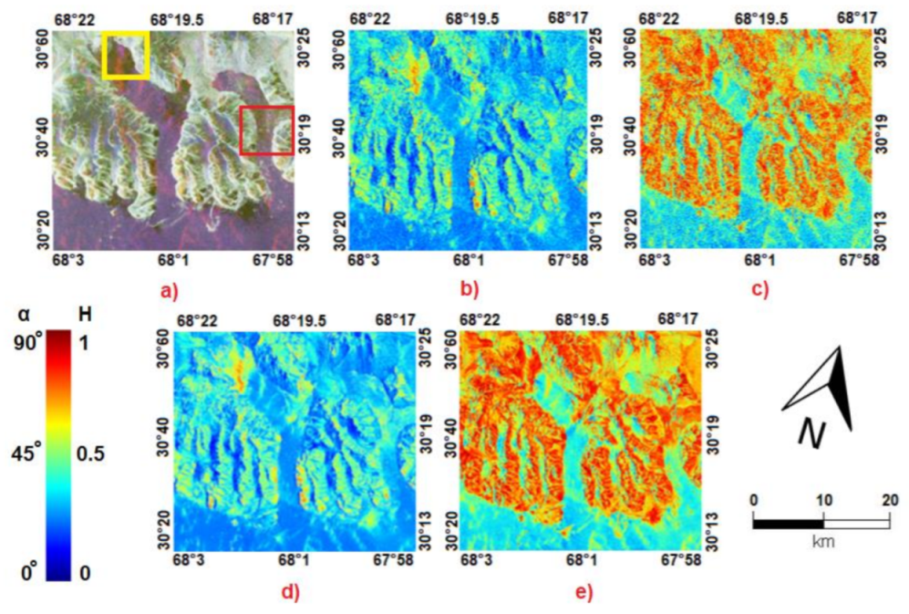
In this section, we present the Pauli RGB images as a reference for the detector analysis. These images were also presented in our previous paper [22]. Figure 2 presents the Pauli RGB for Blosseville, Figure 3 presents Nuugaatsiaq, Figure 4 presents Isortoq and Figure 5 presents Savissivik. RGB images are composed of the three intensities (colours) of the Pauli components: red = HH + VV, green = HH − VV and blue = 2HV. Iceberg identification was similar to our previous work [22]. Here, we used visual analysis to identify icebergs based on whether an iceberg was a bright spot on an image, or had a shadow. We also excluded other targets such as ships, islands and buoys from the analysis whether it was suspected that a target was not an iceberg. For example, ships tend to present as elongated targets on an image. The alpha and entropy are calculated using the Cloude–Pottier eigenvalue/eigenvector polarimetric decomposition [41]. In this case, the entropy is calculated as the logarithmic sum of the eigenvalues of the covariance matrix. Entropy refers to the randomness of the scattering behaviour and can be used to estimate whether polarimetric targets are depolarised or have a more dominant scattering mechanism. Alpha is calculated from the eigenvectors of the covariance matrix. It is related to the incidence angle and dielectric constant of the scatterers [42]. Therefore, it can be used to determine a particular scattering mechanism (odd bounce, even bounce, dihedral scattering). Within sea ice, we focused on bright pixels to identify any icebergs embedded within floes. We also indicate the coastline with a red line in the images. It should be noted that in Figure 5, Blosseville Coast S is not included in our analysis. We will call the image for Blosseville Coast N [22] as Blosseville for short. In Figure 2, a yellow box indicates the area used for detection imaging in Figures 8–10.
4.2. Identifying Targets and Clutter
Icebergs were visually identified in images using RGB images in which the contrast could be adjusted accordingly. It is important to note that due to missing in situ validation data, this analysis is restricted to icebergs that can be identified through visual analysis, so we cannot reliably detect smaller icebergs (<120 m). In order to evaluate the statistics for probability of false alarms (PF), we considered areas inside images that were presenting either open ocean or sea ice. Figure 6 shows the clutter area as a red polygon and icebergs as yellow dots for Blosseville. Nuugaatsiaq and Isortoq, and Savissivik. As we can see, the clutter in Blosseville and Nuugaatsiaq is open ocean, while in Isortoq and Savissivik it is sea ice. Note that in Figure 6a, azimuth ambiguities are visible in the centre to the left of the glacier tongues and just below the clutter area. These are caused by the elevation of the mountains by the coastline. It should also be noted that in Isortoq, the icebergs are indicated by blue dots, and in Savissivik, the green areas. In total, we selected 3242 icebergs for this analysis.
4.3. Preliminary Detection Comparison
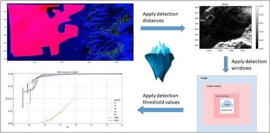
Here, we show the comparison of the different detectors in three polarimetric modes, quad-polarisation, dual-polarisation and single-polarisation. We will first present the detector images for a qualitative assessment over a zoomed area and after that, receiver operating characteristic (ROC) curves for a quantitative assessment. Dual-polarimetric detection is achieved by using the channels HH and HV to work with the detectors designed only for dual-polarimetric data. Single-polarimetric intensities are achieved by focusing on the C11, C22, C33, T11 and T22 elements of the covariance and coherency matrices. All detection images have been created using a window size for the target area or 5 × 5 and (when required) a clutter area of 105 × 105 pixels using a guard window of 35 × 35. Figure 7 represents the guard window approach we used. In the following, we will also test changes in this window configuration.
Detection Distances
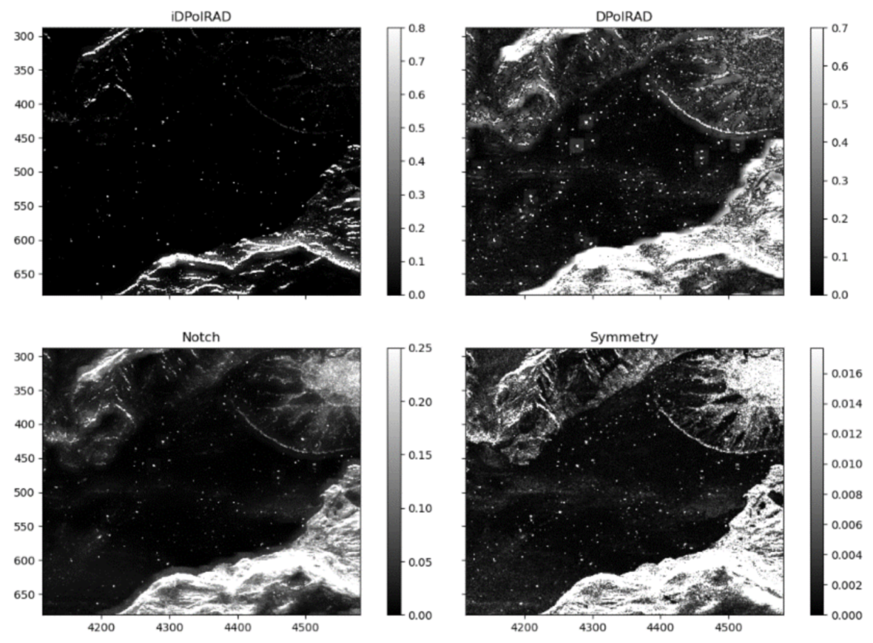
Here, we show the images of detection thresholds that are set as distances generated by the detector algorithms. This method allows for a preliminary understanding of the detection capabilities and the contrast without having to select threshold values. We apply threshold values afterwards to generate results in Section 5. Figure 8 shows iDPolRAD, DPolRAD, n filter and symmetry detection images for Blosseville. Please note: land (bottom and top of the image) will be detected too, but we can exclude it using land masks. If we look at the images, we seem to have the clearest detection using the reflection symmetry detector followed by the notch filter and the DPolRAD close behind. The next images in Figure 9 show parameters from the Cloude–Pottier decomposition, with alpha, entropy, first eigenvalue (λ1) and third eigenvalue (λ3) [6].
From the images, it is clear that the alpha and entropy are not perfect detectors. Rather, they are better to show classification of sea ice as in Section 4.1. λ1 and λ3 seem to be more suited for the detection task. The images in Figure 10 show the first (σ1) and third (σ3) eigenvalues from the PMF, then the PWF and the OPD.
From the images, it is clear that σ1, the PWF and the OPD detectors tend to give the visually best performance, while σ3 is missing many icebergs. Detector output shows similar trends in other locations. It is clear that a quantitative analysis is needed to evaluate the performance in a better way. This follows in the next section.
5. Results
In this section, we present the ROC curves. These are plots of probability of detection (PD) against probability of false alarms (PF). We first present the quad-polarimetric results, and then move to dual-polarimetric and single-polarimetric results. We will first show the ROC curves and then summarise them in tables in next section.
5.1. Quad-Polarimetric ROC Curves
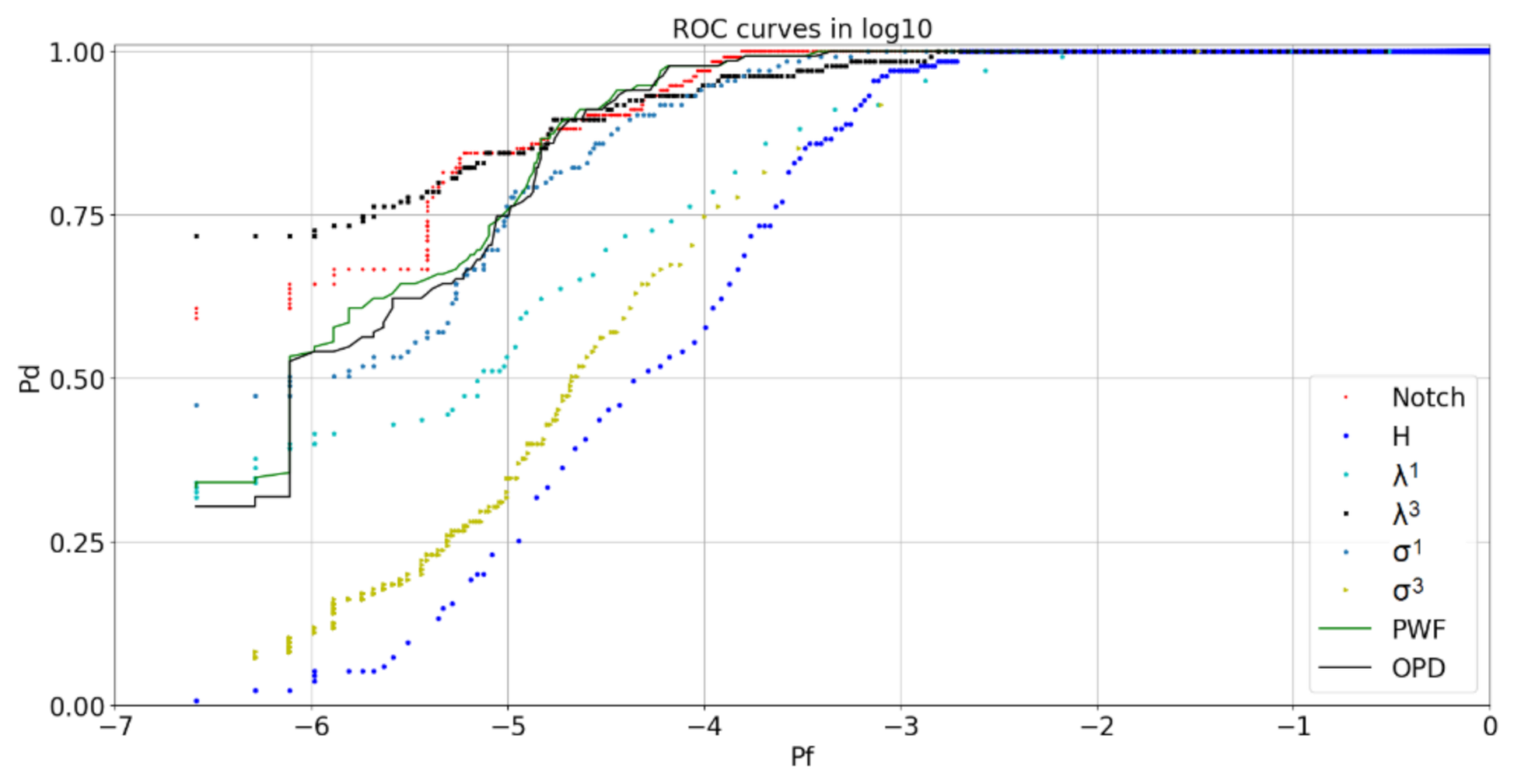
Figure 11 presents a ROC curve for the case of open ocean clutter (Blosseville and Nuugaatsiaq) using a target window size of 5 × 5 and a clutter window size of 105 × 105.
From Figure 11, we can see that in case of open ocean, σ3 of the PMF does not perform properly. This is expected, since icebergs are brighter than the background in most open ocean conditions. All the other detectors provide a similar performance, but we can see some differences when we consider different levels of false alarm rates.
(1)
Here, we can see that the PWF and the OPD both seem to provide the best performance (0.990) followed by σ1, the notch filter, entropy, λ3 and λ1. The worst performance is σ3 of the PMF, with a PD of 0.034.
(2)
Here, the best detector is the entropy (0.808) followed by λ3, the PWF, σ3, the OPD, and the notch filter. The worst performance is λ1 (0.345).
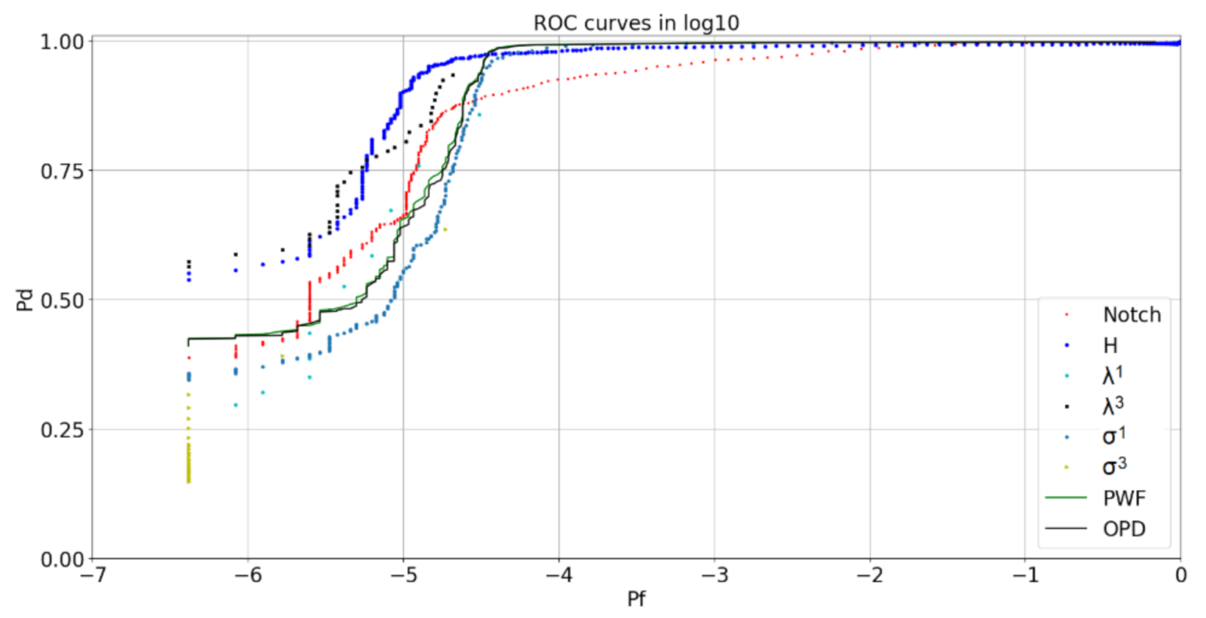
Figure 12 presents a ROC for the case of sea ice (Isortoq and Savissivik).
Interestingly, we can see that in Figure 15, the entropy performance declines, which is most likely due to the number of scatterers present in the sea ice, which increases their entropy. Other adaptive detectors (e.g., the PMF, the PWF, and the PNF) also show a decreased performance in sea ice, since they are detecting heterogeneity of the sea ice.
(1)
The best detector is the λ3 eigenvalue with PD equal to 0.770. This is followed by the notch filter, λ1, the PWF, the OPD, σ1 and σ3. The worst performance is the entropy (0.074).
(2)
Here, the performance degrades, but λ3 remains the best detector, with a PD of 0.770. This is followed by λ1, the notch filter, the PWF, the OPD, and σ1, with no result for σ3. The entropy shows the worst overall performance, with a PF of 0.015.
We now want to test in a different clutter window. We show the quad-polarimetric ROC curves with a target window of 15 × 15 and a train window of 255 × 255 window, including a guard of 205 × 205 pixels (Figure 13 and Figure 14).
It is interesting to see that by using a larger window, the performance has been reduced. This is because the icebergs analysed here are particularly small (<120 m) and a larger window seems to impede detection. For instance, in open oceans, some of the smaller icebergs can only be detected with probability of false alarms proximal to 1.
5.2. Dual-Polarimetric ROC Curves
For the dual-polarimetric ROC curves, we present the same window size with a guard window, but this time we are only considering three elements of the covariance matrix C11, C22 and C12 for analysis. This means that only the images HH and HV are used. Figure 17 shows a dual-polarimetric ROC curve with a 5 × 5 target window, a 35 × 35 guard window size and a 105 × 105 clutter window size. All the dual-polarimetric detectors tested provide relatively similar performances. Again, we want to analyse performances using two different levels of false alarm rates.
(1)
The PWF provides the best performance (0.990) followed by σ1, the OPD, the notch and both the DPolRAD and the iDPolRAD. The reflection symmetry detector has the worst performance (0.969). No performance is shown from σ3 because in dual-polarimetric detection, we do not have the third eigenvalues.
(2)
When compared to the quad-polarimetric results, we can see a substantial difference in PD values. The reflection symmetry detector becomes the best detector (0.612) followed by the PWF, the OPD, σ1, the DPolRAD, the iDPolRAD and the notch filter with the worst performance (0.451).
Figure 18 presents the same result with sea ice clutter. Note that we can see differences between quad and dual for all levels of PF.
(1)
Here, we can see that the DPolRAD provides the best performance (0.874) followed by the symmetry, the iDPolRAD, the PWF, σ1, and the OPD. The notch filter has the worst performance (0.793).
(2)
Here, we can see that there is a range of PD values for all the detectors. The DPolRAD and the iDPolRAD show the best performance (0.593). This is followed by the notch filter and σ1, PWF and symmetry. The OPD detector appears to show the worst performance, with a PD value of 0.313.
The first thing to notice from Figure 17 and Figure 18 is that the notch filter gives an improved performance in sea ice, to the quad-polarimetric version, which helps understand how the improved power of some adaptive detectors may produce several false alarms when there is sea ice. Performance between other detectors is also similar, with, PWF showing the best performance (0.990) in open ocean when PF is 10−5. The DPolRAD slightly outperforms with a PD of 0.874 in sea ice when PF is 10−5. As an important finding, we show that the dual-polarimetric performance is overall lower than the quad-polarimetric performance.
5.3. Intensities ROC Curves
In this section, we investigate detectors set with intensity of backscattering representing an appropriate scattering mechanism. These certainly include the single-polarimetric detectors when we use the co-polarisation or cross-polarisation channels on their own. However, they also include quad-polarimetric detectors when we consider coherence combinations of co-polarisation channels. We show ROC curves in Figure 19 and Figure 20 using C11, C22 and C33, plus T11 and T22 images. We apply to a window of 5 × 5. Again, we want to analyse performances using two different levels of false alarm rates.
(1)
The HV cross-channel seems to provide the best performance (0.989) followed by HH, HH + VV and HH − VV. The VV channel gives the worst performance (0.851). In open ocean, there is not a significant difference in performance compared to the dual-polarimetric results.
(2)
Here, the performance degrades and HH − VV shows the best performance (0.822) followed by HH, and HV with the worst performance (0.624). Now the difference is much more apparent in all the channels except HH − VV, but this requires quad-polarimetric analysis as above.
Figure 20 shows the ROC performance in sea ice clutter. Again, we want to analyse performances using two different levels of false alarm rates.
(1)
Here, we can see that the VV channel provides the best performance (0.719) followed in order by HV, HH + VV and HH − VV with the worst performance (0.561). No matter what PF value, the performance has declined.
(2)
The performance here has degraded, with HH − VV providing the best performance (0.334) followed only by HV (0.255).
5.4. Best Detectors
Table 2 and Table 3 summarise the results and reveal that the best detectors for quad-polarimetric appear to be the PWF, the OPD and σ1 detectors, with the worst performance from the σ3 in open ocean, and entropy in sea ice. Table 4 and Table 5 show that the best detectors for dual-polarimetric detection again appear to be the OPD and the PWF in open ocean. However, for sea ice, the best detectors appear to be the reflection symmetry detector and the DPolRAD. Finally, Table 6 and Table 7 show that the best detection intensity appears to be the HV channel when the detection is easier and the HH − VV channel in more complex environments. Note that numbers in green represent the highest PD values after fixing the PF.
6. Discussion
In this section, we outline and evaluate the results of the analysis.
Using a target window of 5 × 5 and clutter window of 105 × 105, the ROC curves suggest that the best performance for detecting icebergs in open ocean provides a PD of 0.99 with a PF of 10−5 or 0.81 for PF 10−6. When we compare with iceberg detection in sea ice with the same false alarm rate, we have a PD of 0.9 and 0.77, respectively, indicating that detection in sea ice is more complex. This can be explained by the fact that sea ice can trigger false alarms, especially in more powerful detectors [13].
Interestingly, we can see that performance evaluation in dual-polarimetric detectors shows a reduction in PD for small values of false alarms. For instance, fixing PF to 10−6, the PD is 0.61 in open ocean and 0.59 in sea ice. This is in line with the fact that by reducing the number of polarisation channels, our discrimination capability is reduced. However, in open ocean, the detection task is easier and we use larger values of PF. As a result, the difference in performance between dual and quad detection is very limited.
Results from detectors based on intensities show again that in easier scenarios (such as in open ocean), where PF = 10−5, the difference is minor, with HV reaching a PD of 0.985 (compared to 0.99 for quad). However, when more complex scenarios are considered (such as in sea ice), the performance of HV degrades and a quad-polarimetric detector performs better. For instance, with PF = 10−6 in open ocean, the VV channel shows PD = 0.78 (compared to 0.99 of quad); and within sea ice in the same channel, the PD values are 0.71 for PF = 10−5 (compared to 0.90 of quad) and 0.25 for PF = 10−6 (compared to 0.77 of quad).
To summarise, when the detection task is easier because larger icebergs in open ocean are easier to visualise, a single-polarisation channel will perform relatively similarly to a quad-polarimetric one. However, for the detection of icebergs in sea ice or for smaller icebergs (smaller false alarm rate), adding polarimetric information will help. Finally, we saw that when we increase the target window to 15 × 15 and clutter window to 255 × 255, the PD value reduces. This is in line with the fact that when we use a bigger window, more pixels are included, thus the target is smeared (when averaging), and the probability of detection is reduced. Moreover, when ring windows are not used, then the results show a degradation of performance. The absolute values for PD need to be taken with care since we only restricted the analysis to the icebergs that are clearly identifiable. However, the relative comparison of detectors should still be preserved if fainter icebergs were introduced. It should also be noted that additional data to determine whether detection is impeded by temperature or precipitation in winter and summer was not available.
7. Conclusions
In this work, we tested an ALOS-2 dataset with six state-of-the art detectors, most of them designed to be used for ship detection. The detectors are the intensity dual-polarisation ratio anomaly detector (iDPolRAD), the polarimetric notch filter (PNF), the polarimetric match filter (PMF), the reflection symmetry detector, the multi-look polarimetric whitening filter (MPWF) and the optimal polarimetric detector (OPD). We estimated detection performance over four ALOS-2 quad-polarimetric single-look complex SAR images, in four locations in Greenland. To compare the performances of each detector, we performed the analysis using two scenarios. Two of the images had icebergs in an open ocean setting, and two showed icebergs embedded within sea ice. In total, we considered 3,242 icebergs in this analysis. We show that, overall, the quad-polarimetric detectors, the OPD and the PWF, provide the best detection performance, with a PD of 0.99 in open ocean when the false alarm is set to 10−5. However, in sea ice, λ3 shows the best performance (0.90). For dual-polarimetric performance, we conclude that the PWF gives the best performance in open ocean (0.90). In the sea ice, the best detector is the DPolRAD (0.978). Finally, we tested the data in the single-polarisation mode, showing that the best performance is HV in the open ocean (0.99) and in the sea ice (0.87). The differences between quad- and dual- or single-polarimetric detectors are more evident with low detection probabilities set at PF = 10−6 when compared to the HV channel as quad-polarimetric detectors increase the PD from 0.62 to 0.81 for open ocean and from 0.26 to 0.77 for sea ice.
Author Contributions
Conceptualization, J.B. and A.M.; methodology, J.B.; software, A.M.; validation, J.B., A.M. and V.A.; formal analysis, J.B.; investigation, J.B; resources, A.M.; data curation, J.B.; writing—original draft preparation, J.B.; writing—review and editing, J.B. and V.A.; visualization, J.B.; supervision, A.M.; project administration, J.B. All authors have read and agreed to the published version of the manuscript.
Funding
This research received no external funding.
Acknowledgments
All data were provided by the project number 1151. ALOS-2 Product-JAXA 2017, all rights reserved.
Conflicts of Interest
The authors do not declare any conflicts of interest.
References
- Hanna, E.; Mernild, S.H.; Cappelen, J.; Steffen, K. Recent warming in Greenland in a long-term instrumental (1881–2012) climatic context: I. Evaluation of surface air temperature records. Environ. Res. Lett. 2012, 7, 045404. [Google Scholar] [CrossRef]
- Akbari, V.; Brekke, C. Iceberg detection in open water and sea ice using C-band radar polarimetry. In Proceedings of the 2017 IEEE International Geoscience and Remote Sensing Symposium (IGARSS), Fort Worth, TX, USA, 23–28 July 2017; pp. 2298–2301. [Google Scholar]
- Bigg, G.R. Icebergs: Their Science and Links to Global Change; Cambridge University Press: Cambridge, UK, 2015. [Google Scholar]
- Frost, A.; Ressel, R.; Lehner, S. Automated iceberg detection using high-resolution X-band SAR images. Can. J. Remote Sens. 2016, 42, 354–366. [Google Scholar] [CrossRef] [Green Version]
- Wesche, C.; Dierking, W. Estimating iceberg paths using a wind-driven drift model. Cold Reg. Sci. Technol. 2016, 125, 31–39. [Google Scholar] [CrossRef]
- Cloude, S. Polarisation: Applications in Remote Sensing; Oxford University Press: New York, NY, USA, 2010. [Google Scholar]
- Heiselberg, H. Ship-iceberg classification in SAR and multispectral satellite images with neural networks. Remote Sens. 2020, 12, 2353. [Google Scholar] [CrossRef]
- Lopez-Lopez, L.; Parmiggiani, F.; Moctezuma-Flores, M.; Guerrieri, L. SAR image observations of the A-68 iceberg drift. Cryosphere Discuss. 2020, 1–16. [Google Scholar]
- Heiselberg, H. Ship-iceberg detection & classification in sentinel-1 SAR images. TransNav Int. J. Mar. Navig. Saf. Sea Transp. 2020, 14, 235–241. [Google Scholar]
- Powell, R.; Domack, G.W. Modern glaciomarine environments. In Modern and Past Glacial Environments; Elsevier: Amsterdam, The Netherlands, 2002; pp. 361–389. [Google Scholar]
- Wadhams, P.; Woodwort-Lynas, C. Icebergs; Butterworth-Heinemann Limited: Oxford, UK, 2004. [Google Scholar]
- Akbari, V.; Brekke, C.; Doulgeris, A.P.; Storvold, R.; Sivertsen, A.H. Quad-polarimetric SAR for detection and characterization of icebergs. In Proceedings of the ESA Living Planet Symposium 2016, Prague, Czech Republic, 9–13 May 2016. [Google Scholar]
- Marino, A.; Dierking, W.; Wesche, C. A depolarization ratio anomaly detector to identify icebergs in sea ice using dual-polarization SAR images. IEEE Trans. Geosci. Remote Sens. 2016, 54, 5602–5615. [Google Scholar] [CrossRef] [Green Version]
- Marino, A. A notch filter for ship detection with polarimetric SAR data. IEEE J. Sel. Top. Appl. Earth Obs. Remote Sens. 2013, 6, 1219–1232. [Google Scholar] [CrossRef] [Green Version]
- Novak, L.M.; Sechtin, M.B.; Cardullo, M.J. Studies of target detection algorithms that use polarimetric radar data. IEEE Trans. Aerosp. Electron. Syst. 1989, 25, 150–165. [Google Scholar] [CrossRef] [Green Version]
- Nunziata, F.; Migliaccio, M.; Brown, C.E. A physically-based approach to observe man-made metallic objects in dual-polarized SAR data. In Proceedings of the 2010 IEEE International Geoscience and Remote Sensing Symposium, Honolulu, HI, USA, 25–30 July 2010; pp. 3007–3010. [Google Scholar]
- Chaney, R.; Bud, M.; Novak, L. On the performance of polarimetric target detection algorithms. IEEE Aerosp. Electron. Syst. Mag. 1990, 5, 10–15. [Google Scholar] [CrossRef]
- Novak, L.M.; Burl, M.C. Optimal speckle reduction in polarimetric SAR imagery. IEEE Trans. Aerosp. Electron. Syst. 1990, 26, 293–305. [Google Scholar] [CrossRef]
- Soldal, I.H.; Dierking, W.; Korosov, A.; Marino, A. Automatic Detection of Small Icebergs in Fast Ice Using Satellite Wide-Swath SAR Images. Remote Sens. 2019, 11, 806. [Google Scholar] [CrossRef] [Green Version]
- Crisp, D.J. The State-of-the-Art in Ship Detection in Synthetic Aperture Radar Imagery; DSTO-RR-0272; Defence Science And Technology Organisation Edinburgh: Edinburgh, Australia, 2004. [Google Scholar]
- Dierking, W.; Wesche, C. C-band radar polarimetry—Useful for detection of icebergs in sea ice? IEEE Trans. Geosci. Remote Sens. 2013, 52, 25–37. [Google Scholar] [CrossRef]
- Bailey, J.; Marino, A. Quad-Polarimetric Multi-Scale Analysis of Icebergs in ALOS-2 SAR Data: A Comparison between Icebergs in West and East Greenland. Remote Sens. 2020, 12, 1864. [Google Scholar] [CrossRef]
- Jagdhuber, T.; Stockamp, J.; Hajnsek, I.; Ludwig, R. Identification of soil freezing and thawing states using SAR polarimetry at C-band. Remote Sens. 2014, 6, 2008–2023. [Google Scholar] [CrossRef] [Green Version]
- Park, S.-E. Variations of microwave scattering properties by seasonal freeze/thaw transition in the permafrost active layer observed by ALOS PALSAR polarimetric data. Remote Sens. 2015, 7, 17135–17148. [Google Scholar] [CrossRef] [Green Version]
- Muhuri, A.; Manickam, S.; Bhattacharya, A. Scattering mechanism based snow cover mapping using RADARSAT-2 C-Band polarimetric SAR data. IEEE J. Sel. Top. Appl. Earth Obs. Remote Sens. 2017, 10, 3213–3224. [Google Scholar] [CrossRef]
- Touzi, R. Target scattering decomposition in terms of roll-invariant target parameters. IEEE Trans. Geosci. Remote Sens. 2006, 45, 73–84. [Google Scholar] [CrossRef]
- Willis, C.; Macklin, J.; Partington, K.; Teleki, K.; Rees, W.; Williams, R. Iceberg detection using ERS-1 synthetic aperture radar. Int. J. Remote Sens. 1996, 17, 1777–1795. [Google Scholar] [CrossRef]
- Wesche, C.; Dierking, W. Iceberg signatures and detection in SAR images in two test regions of the Weddell Sea, Antarctica. J. Glaciol. 2012, 58, 325–339. [Google Scholar] [CrossRef] [Green Version]
- Gladstone, R.; Bigg, G. Satellite tracking of icebergs in the Weddell Sea. Antarct. Sci. 2002, 14, 278–287. [Google Scholar] [CrossRef]
- Collares, L.L.; Mata, M.M.; Kerr, R.; Arigony-Neto, J.; Barbat, M.M. Iceberg drift and ocean circulation in the northwestern Weddell Sea, Antarctica. Deep Sea Res. Part II Top. Stud. Oceanogr. 2018, 149, 10–24. [Google Scholar] [CrossRef]
- Yamaguchi, Y. Polarimetric SAR Imaging: Theory and Applications; CRC Press: Boca Raton, FL, USA, 2020. [Google Scholar]
- Akbari, V.; Doulgeris, A.P.; Eltoft, T. Non-Gaussian clustering of SAR images for glacier change detection. In Proceedings of the ESA Living Planet Symposium, Bergen, Norway, 28 June–2 July 2010. [Google Scholar]
- Lee, J.-S.; Jurkevich, L.; Dewaele, P.; Wambacq, P.; Oosterlinck, A. Speckle filtering of synthetic aperture radar images: A review. Remote Sens. Rev. 1994, 8, 313–340. [Google Scholar] [CrossRef]
- Chen, J.Y.; Reed, I.S. A detection algorithm for optical targets in clutter. IEEE Trans. Aerosp. Electron. Syst. 1987, 1, 46–59. [Google Scholar] [CrossRef]
- Liu, G.; Huang, S.; Torre, A.; Rubertone, F. The multilook polarimetric whitening filter (MPWF) for intensity speckle reduction in polarimetric SAR images. IEEE Trans. Geosci. Remote Sens. 1998, 36, 1016–1020. [Google Scholar]
- Lopes, A.; Séry, F. Optimal speckle reduction for the product model in multilook polarimetric SAR imagery and the Wishart distribution. IEEE Trans. Geosci. Remote Sens. 1997, 35, 632–647. [Google Scholar] [CrossRef]
- Khan, S.; Guida, R. On fractional moments of multilook polarimetric whitening filter for polarimetric SAR data. IEEE Trans. Geosci. Remote Sens. 2013, 52, 3502–3512. [Google Scholar] [CrossRef] [Green Version]
- Akbari, V.; Anfinsen, S.N.; Doulgeris, A.P.; Eltoft, T. A change detector for polarimetric SAR data based on the relaxed Wishart distribution. In Proceedings of the 2015 IEEE International Geoscience and Remote Sensing Symposium (IGARSS), Milan, Italy, 26–31 July 2015; pp. 3806–3809. [Google Scholar]
- Galland, F.; Nicolas, J.-M.; Sportouche, H.; Roche, M.; Tupin, F.; Réfrégier, P. Unsupervised synthetic aperture radar image segmentation using Fisher distributions. IEEE Trans. Geosci. Remote Sens. 2009, 47, 2966–2972. [Google Scholar] [CrossRef]
- Bjørk, A.A.; Kruse, L.; Michaelsen, P. Brief communication: Getting Greenland’s glaciers right–a new data set of all official Greenlandic glacier names. Cryosphere 2015, 9, 2215–2218. [Google Scholar] [CrossRef] [Green Version]
- Cloude, S.R.; Pottier, E. A review of target decomposition theorems in radar polarimetry. IEEE Trans. Geosci. Remote Sens. 1996, 34, 498–518. [Google Scholar] [CrossRef]
- Cloude, S.R.; Pottier, E. An entropy based classification scheme for land applications of polarimetric SAR. IEEE Trans. Geosci. Remote Sens. 1997, 35, 68–78. [Google Scholar] [CrossRef]
Figure 1.
Google Earth image of data acquisition. Red boxes indicate the image footprints. Yellow numbers correspond to the image IDs in Table 1. Compass point indicates north. Scale: 900 m. Reprinted with permission from ref. [22] Copyright 2020 Remote Sensing

Figure 2.
Output images for Blosseville, 15 August 2015 01:26: (a) Pauli RGB image with extent shown, (b) alpha image in a 5 × 5 window, (c) entropy image in a 5 × 5 window, (d) alpha image in an 11 × 11 window, and (e) entropy image in an 11 × 11 window. The red box indicates the extent of previous analysis in this location. The yellow box indicates the area used in the detection tests. Adapted with permission from ref. [22]. Copyright 2020 Remote Sensing.

Figure 3.
Output images for Nuugaatsiaq, 15 August 2015 01:26: (a) Pauli RGB image, (b) alpha image in a 5 × 5 window, (c) entropy image in a 5 × 5 window, and (d) visual identification of icebergs and land mask. Yellow dots are icebergs. The red line represents the shoreline. Reprinted with permission from ref. [22] Copyright 2020 Remote Sensing.

Figure 4.
Output images for Isortoq, 15 August 2015 01:26, (a) Pauli RGB image, (b) alpha image in a 5 × 5 window, (c) entropy image in a 5 × 5 window, (d) visual identification of icebergs and land mask Yellow dots are icebergs. The red line represents the shoreline. Reprinted with permission from ref. [22] Copyright 2020 Remote Sensing.

Figure 5.
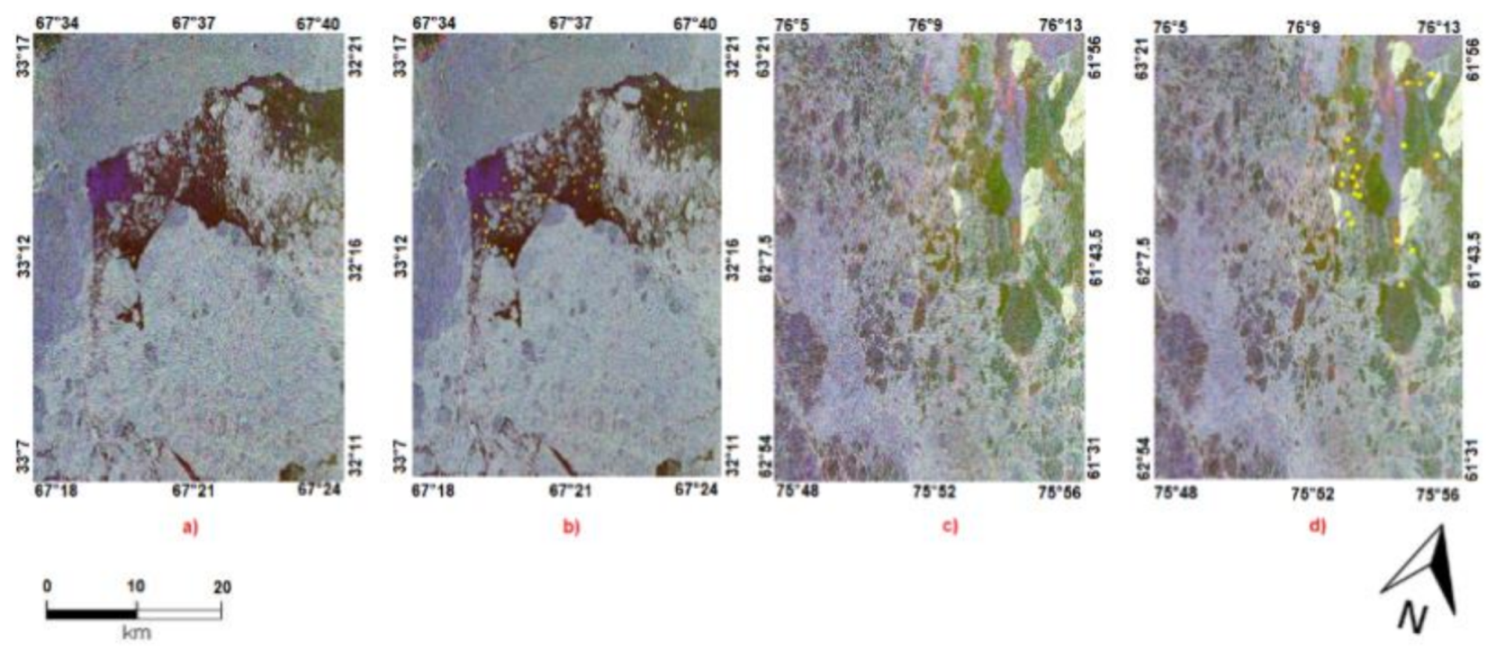
Output images for (a) Blosseville Coast S Pauli RGB image 20 June 2015 01:26, (b) Blosseville Coast S visual analysis, (c) Savissivik RGB image 6 December 2017 02:52, and (d) Savissivik visual analysis. Yellow dots are icebergs. Note that Blosseville Coast S is not used in this paper. Reprinted with permission from ref. [22] Copyright 2020 Remote Sensing.
Figure 5.
Output images for (a) Blosseville Coast S Pauli RGB image 20 June 2015 01:26, (b) Blosseville Coast S visual analysis, (c) Savissivik RGB image 6 December 2017 02:52, and (d) Savissivik visual analysis. Yellow dots are icebergs. Note that Blosseville Coast S is not used in this paper. Reprinted with permission from ref. [22] Copyright 2020 Remote Sensing.

Figure 6.
Pauli images of each location. (a) Target and clutter mask for Blosseville. Scenario is a mix of open ocean, and glacier tongues. Azimuth ambiguities are present in the middle of the image. (b) Nuugaatsiaq. Scenario is a mix of open ocean, and islands. (c) Isortoq. Scenario is a mix of sea ice and ice floes. Note blue dots for icebergs. (d) Savissivik. Scenario is mainly sea ice, with embedded targets, and green areas indicate icebergs. Red polygons indicate clutter.

Figure 7.
The guard window approach. The blue area represents image pixels, the light pink area represents the clutter window, and the dark pink area represents the guard window, to eliminate background clutter from the target window (white). In the case of this analysis, the target is an iceberg.
Figure 7.
The guard window approach. The blue area represents image pixels, the light pink area represents the clutter window, and the dark pink area represents the guard window, to eliminate background clutter from the target window (white). In the case of this analysis, the target is an iceberg.

Figure 8.
Iceberg detection iDPolRAD, DPolRAD, notch filter and symmetry for Blosseville. Image size is 350 × 500 pixels. Greyscales indicate detection intensity.
Figure 8.
Iceberg detection iDPolRAD, DPolRAD, notch filter and symmetry for Blosseville. Image size is 350 × 500 pixels. Greyscales indicate detection intensity.

Figure 9.
Iceberg detection entropy H, alpha, λ1 and λ3 for Blosseville. Image size is 350 × 600 pixels. Greyscales indicate detection intensity.
Figure 9.
Iceberg detection entropy H, alpha, λ1 and λ3 for Blosseville. Image size is 350 × 600 pixels. Greyscales indicate detection intensity.

Figure 10.
Iceberg detection σ1, σ3, the PWF, and the OPD for Blosseville. Image size is 400 × 600 pixels. Colourmaps indicate detection intensity.
Figure 10.
Iceberg detection σ1, σ3, the PWF, and the OPD for Blosseville. Image size is 400 × 600 pixels. Colourmaps indicate detection intensity.

Figure 11.
Iceberg detection ROC curves for open ocean, target size 5 × 5, clutter size 105 × 105. Notch means the polarimetric notch filter, H means entropy, λ1 and λ3 are the first and third eigenvalues of the covariance matrix, σ1 and σ3 are from the polarimetric match filter, PWF means the polarimetric whitening filter, and OPD means the optimal polarimetric detector.

Figure 12.
Iceberg detection ROC curves for sea ice, target window 5 × 5, clutter window 105 × 105. Notch means the polarimetric notch filter, H means entropy, λ1 and λ3 are the first and third eigenvalues of the covariance matrix, σ1 and σ3 are from the polarimetric match filter, PWF means the polarimetric whitening filter, and OPD means the optimal polarimetric detector.

Figure 13.
Iceberg detection ROC curves for open ocean, target window 15 × 15, clutter window 255 × 255 with a guard window of 205 × 205. Notch means the polarimetric notch filter, H means entropy, λ1 and λ3 are the first and third eigenvalues of the covariance matrix, σ1 and σ3 are from the polarimetric match filter, PWF means the polarimetric whitening filter, and OPD means the optimal polarimetric detector.

Figure 14.
Iceberg detection ROC curves for sea ice, target window 15 × 15, clutter window 255 × 255 with a guard window of 205 × 205. Notch means the polarimetric notch filter, H means entropy, λ1 and λ3 are the first and third eigenvalues of the covariance matrix, σ1 and σ3 are from the polarimetric match filter, PWF means the polarimetric whitening filter, and OPD means the optimal polarimetric detector.

Figure 15.
Iceberg detection ROC curves for open ocean, target window 5 × 5, clutter window 105 × 105 with no guard window. Notch means the polarimetric notch filter, H means entropy, λ1 and λ3 are the first and third eigenvalues of the covariance matrix, σ1 and σ3 are from the polarimetric match filter, PWF means the polarimetric whitening filter, and OPD means the optimal polarimetric detector.

Figure 16.
Iceberg detection ROC curves for sea ice, target window 5 × 5, clutter window 105 × 105 with no guard window. Notch means the polarimetric notch filter, H means entropy λ1 and λ3 are the first and third eigenvalues of the covariance matrix, σ1 and σ3 are from the polarimetric match filter, PWF means the polarimetric whitening filter, and OPD means the optimal polarimetric detector.

Figure 17.
Iceberg detection dual-polarimetric ROC curves for open ocean, 5 × 5, clutter window size 105 × 105. Sym means symmetry detector. iDPolRAD and DPolRAD mean intensity dual-polarisation ratio anomaly detector, and σ1 is from the polarimetric match filter.
Figure 17.
Iceberg detection dual-polarimetric ROC curves for open ocean, 5 × 5, clutter window size 105 × 105. Sym means symmetry detector. iDPolRAD and DPolRAD mean intensity dual-polarisation ratio anomaly detector, and σ1 is from the polarimetric match filter.

Figure 18.
Iceberg detection dual-polarimetric ROC curves for sea ice, 5 × 5, clutter window size 105 × 105. Sym means symmetry detector. iDPolRAD and DPolRAD mean intensity dual-polarisation ratio anomaly detector, σ1 is from the polarimetric match filter.
Figure 18.
Iceberg detection dual-polarimetric ROC curves for sea ice, 5 × 5, clutter window size 105 × 105. Sym means symmetry detector. iDPolRAD and DPolRAD mean intensity dual-polarisation ratio anomaly detector, σ1 is from the polarimetric match filter.

Figure 19.
Iceberg detection intensity ROC curves for open ocean, 5 × 5, clutter window size 105 × 105. C11 is a HH polarisation, C22 is a cross-polarised HV polarisation, C33 is a VV polarisation, T11 is a HH + VV polarisation and T22 is a HH − VV polarisation.
Figure 19.
Iceberg detection intensity ROC curves for open ocean, 5 × 5, clutter window size 105 × 105. C11 is a HH polarisation, C22 is a cross-polarised HV polarisation, C33 is a VV polarisation, T11 is a HH + VV polarisation and T22 is a HH − VV polarisation.

Figure 20.
Iceberg detection intensity ROC curves for sea ice, 5 × 5, clutter window 105 × 105. C11 is a HH polarisation, C22 is a cross-polarised HV polarisation, C33 is a VV polarisation, T11 is a HH + VV polarisation and T22 is a HH − VV polarisation.
Figure 20.
Iceberg detection intensity ROC curves for sea ice, 5 × 5, clutter window 105 × 105. C11 is a HH polarisation, C22 is a cross-polarised HV polarisation, C33 is a VV polarisation, T11 is a HH + VV polarisation and T22 is a HH − VV polarisation.


Table 1.
ALOS-2/PALSAR-2 image properties. Latitude and longitude use centre degrees, minutes, seconds (DMS) coordinates. Incidence angle range is min, centre, and max to indicate the near, mid and far range of each image. Ground resolution is ALOS-2 quad-polarimetric mode. Time is UTC. Note that Savissivik was acquired in winter months.
| ID | Location | Lat/Lon (DMS) | Resolution (m) | Incidence Angle Range (°) | Date/Time |
|---|---|---|---|---|---|
| (1) ALOS2066231 360-150815 | Blosseville Coast | 68°02′13.2″ N 30°19′58.8″ W | 4.3 × 5.1 | 37, 39, 41.5 | 15 August 2015 01:26 |
| (2) ALOS2064761 430-150805 | Nuugaatsiaq | 71°25′26.4″ N 53°26′52.8″ W | 4.3 × 5.1 | 37, 39, 41.5 | 5 August 2015 02:48 |
| (3) ALOS2064461 300-150803 | Isortoq | 65°07′08.4″ N 39°13′37.2″ W | 4.3 × 5.1 | 37, 39, 41.5 | 3 August 2015 02:07 |
| (4) ALOS2191031 530-171206 | Savissivik | 75°52′19.2″ N 62°10′48″ W | 4.3 × 5.1 | 29, 31, 33.6 | 6 December 2017 02:52 |
Table 2.
Probabilities of detection for quad-polarimetric open ocean. Bold numbers indicate highest PD values.
Table 2.
Probabilities of detection for quad-polarimetric open ocean. Bold numbers indicate highest PD values.
| λ1 | λ3 | H | PNF | σ1 | σ3 | PWF | OPD | |
|---|---|---|---|---|---|---|---|---|
| PF = 16 | 0.345 | 0.800 | 0.809 | 0.412 | 0.668 | 0.671 | 0.663 | |
| PF = 15 | 0.799 | 0.944 | 0.948 | 0.950 | 0.983 | 0.034 | 0.990 | 0.990 |
| PF = 14 | N/A | 0.986 | 0.982 | 0.986 | 0.994 | 0.218 | 0.995 | 0.994 |
Table 3.
Probabilities of detection for quad-polarimetric sea ice. Bold numbers indicate highest PD values.
Table 3.
Probabilities of detection for quad-polarimetric sea ice. Bold numbers indicate highest PD values.
| λ1 | λ3 | H | PNF | σ1 | σ3 | PWF | OPD | |
|---|---|---|---|---|---|---|---|---|
| PF = 16 | 0.570 | 0.770 | 0.015 | 0.541 | 0.222 | 0.296 | 0.244 | |
| PF = 15 | 0.785 | 0.904 | 0.074 | 0.837 | 0.674 | 0.111 | 0.711 | 0.689 |
| PF = 14 | 0.970 | 0.970 | 0.548 | 0.970 | 0.956 | 0.615 | 0.963 | 0.963 |
Table 4.
Probabilities of detection for dual-polarimetric open ocean. Bold numbers indicate highest PD values.
Table 4.
Probabilities of detection for dual-polarimetric open ocean. Bold numbers indicate highest PD values.
| iD | D | PNF | σ1 | Sym | PWF | OPD | |
|---|---|---|---|---|---|---|---|
| PF = 1−6 | 0.462 | 0.487 | 0.451 | 0.535 | 0.612 | 0.551 | 0.542 |
| PF = 1−5 | 0.972 | 0.970 | 0.978 | 0.988 | 0.969 | 0.990 | 0.985 |
| PF = 1−4 | 0.993 | 0.994 | 0.993 | 0.994 | 0.994 | 0.993 |
Table 5.
Probabilities of detection for dual-polarimetric sea ice. Bold numbers indicate highest PD values.
Table 5.
Probabilities of detection for dual-polarimetric sea ice. Bold numbers indicate highest PD values.
| iD | D | PNF | σ1 | Sym | PWF | OPD | |
|---|---|---|---|---|---|---|---|
| PF=1−6 | 0.593 | 0.593 | 0.556 | 0.385 | 0.363 | 0.370 | 0.313 |
| PF=1−5 | 0.837 | 0.874 | 0.793 | 0.808 | 0.867 | 0.815 | 0.800 |
| PF=1−4 | 0.963 | 0.963 | 0.963 | 0.970 | 0.970 | 0.978 | 0.978 |
Table 6.
Probabilities of detection for intensities open ocean. Bold numbers indicate highest PD values.
Table 6.
Probabilities of detection for intensities open ocean. Bold numbers indicate highest PD values.
| HV | HH | VV | HH + VV | HH-VV | |
|---|---|---|---|---|---|
| PF = 1−6 | 0.624 | 0.782 | 0.822 | ||
| PF=1−5 | 0.989 | 0.977 | 0.851 | 0.962 | 0.890 |
| PF=1−4 | 0.995 | 0.993 | 0.911 | 0.982 | 0.930 |
Table 7.
Probabilities of detection for intensities sea ice. Bold numbers indicate highest PD values.
Table 7.
Probabilities of detection for intensities sea ice. Bold numbers indicate highest PD values.
| HV | HH | VV | HH + VV | HH − VV | |
|---|---|---|---|---|---|
| PF = 1−6 | 0.255 | 0.334 | |||
| PF = 1−5 | 0.706 | 0.719 | 0.663 | 0.561 | |
| PF = 1−4 | 0.940 | 0.910 | 0.926 | 0.920 | 0.905 |
Publisher’s Note: MDPI stays neutral with regard to jurisdictional claims in published maps and institutional affiliations. |
© 2021 by the authors. Licensee MDPI, Basel, Switzerland. This article is an open access article distributed under the terms and conditions of the Creative Commons Attribution (CC BY) license (https://creativecommons.org/licenses/by/4.0/).
Share and Cite
MDPI and ACS Style
Bailey, J.; Marino, A.; Akbari, V. Comparison of Target Detectors to Identify Icebergs in Quad-Polarimetric L-Band Synthetic Aperture Radar Data. Remote Sens. 2021, 13, 1753. https://0-doi-org.brum.beds.ac.uk/10.3390/rs13091753
AMA Style
Bailey J, Marino A, Akbari V. Comparison of Target Detectors to Identify Icebergs in Quad-Polarimetric L-Band Synthetic Aperture Radar Data. Remote Sensing. 2021; 13(9):1753. https://0-doi-org.brum.beds.ac.uk/10.3390/rs13091753
Chicago/Turabian StyleBailey, Johnson, Armando Marino, and Vahid Akbari. 2021. "Comparison of Target Detectors to Identify Icebergs in Quad-Polarimetric L-Band Synthetic Aperture Radar Data" Remote Sensing 13, no. 9: 1753. https://0-doi-org.brum.beds.ac.uk/10.3390/rs13091753
Note that from the first issue of 2016, this journal uses article numbers instead of page numbers. See further details here.