
Uncertainty of Drone-Derived DEMs and Significance of Detected Morphodynamics in Artificially Scraped Dunes


1
Department of Physics and Earth Sciences, University of Ferrara, 44122 Ferrara, Italy
2
School of Geography and Earth Sciences, Ulster University, Coleraine BT52 1SA, UK
*
Author to whom correspondence should be addressed.
Remote Sens. 2021, 13(9), 1823; https://0-doi-org.brum.beds.ac.uk/10.3390/rs13091823
Submission received: 31 March 2021
/
Revised: 26 April 2021
/
Accepted: 4 May 2021
/
Published: 7 May 2021
(This article belongs to the Special Issue UAV Application for Monitoring Coastal Morphology)
Abstract
:This work capitalises on the morphodynamic study of a scraped artificial dune built on the sandy beach of Porto Garibaldi (Comacchio, Italy) as a barrier to protect the touristic facilities from sea storms during the winter season and contributes to understanding of the role of elevation data uncertainty and uniform thresholds for change detection (TCDs) on the interpretation of volume change estimations. This application relies on products derived from unmanned aerial vehicle (UAV) surveys and on the evaluation of the uncertainty associated with volume change estimations to interpret the case study morphodynamics under non-extreme sea and wind conditions. The analysis was performed by comparing UAV-derived digital elevation models (DEMs)—root mean squared error (RMSE) vs. global navigation satellite system (GNSS) < 0.05 m—and orthophotos, considering the significance of the identified changes by applying a set of TCDs. In this case, a threshold of ~0.15 m was able to detect most of the morphological variations. The set of TCD ≤ 0.15 m was considered to discuss the significance of minor changes and the uncertainty of volume change calculations. During the analysed period (21 December 2016–20 January 2017), water levels and waves affected the front of the artificial dune by eroding the berm area; winds remodelled the entire dune, moving the loose sand around the dune and further inland; sediment volumes mobilised by sea and wind forcing were comparable. This work suggests that UAV-derived coastal morphological variations should be interpreted by integrating: (i) a set of uniform thresholds to detect significant changes; (ii) the uncertainty generated by the propagation of the original uncertainty of the elevation products; (iii) the characteristics of the morphodynamic drivers evaluated by adopting uncertainty-aware approaches. Thus, the contribution of subtle morphological changes—magnitudes comparable with the instrumental accuracy and/or the assessed propagated uncertainty—can be properly accounted for.
1. Introduction
Beaches with high touristic appeal are often intensely managed in order to preserve their recreational and commercial functionalities. In addition to building on them, man can modify the beach morphology to obtain specific advantages, such as an increased protection from coastal storms. However, these actions also affect the local morphodynamics, as in the case of scraped artificial dunes. A specific study case of the latter, from the Northern Adriatic Italian coast (Figure 1), is presented in this paper by discussing its morphodynamics in relation to the uncertainty of drone-derived elevation data and the significant morphological variation identified by applying a set of thresholds on vertical changes.
1.1. Artificial Dunes and Beach Scraping
Artificial dunes are human-made sandy features built on an emerged beach to protect the inner part of the coast and its assets. Acting as barriers and sand deposits, they offer an effective countermeasure to flooding and erosion when properly designed (Bruun, 1983 [1]). The so-called “winter dune” investigated in this study—unlike the artificial dunes in Figure 2a and b that are examples of long-/medium-term measures—is a temporary small-scale measure put in place as a seasonal protective measure. Every autumn before the storm season, it is built at several locations along the Emilia-Romagna (Italy) coast (Figure 1 and Figure 2c,d) and is dismantled in spring before the touristic season begins (Harley and Ciavola, 2013 [2]). Temporary dunes or embankments are generally built by beach scraping (see examples in Figure 2c,d), which consists of moving the sand of the beach from where a surplus is available to the desired position by means of machines, such as bulldozers (Bruun, 1983 [1]). This represents the most commonly applied approach (e.g., Bruun, 1983; Wells and McNinch, 1991; Harley and Ciavola, 2013; Cooke et al., 2012 [1,2,3,4]) when enough sediment is available, as it is fast and non-expensive compared to building dunes with nourished sand.
The morphodynamic response of scraped beaches has been thoroughly studied over the years, highlighting both positive and negative effects. It is clear that scraped dunes do not replicate natural dunes, and their behaviour may consistently differ (Smyth and Hesp (2015) [5]; Ellis and Román-Rivera, 2019 [6]). Nonetheless, scraping represents an effective way to provide temporary protection for properties (e.g., Kelley, 2013; Harley and Ciavola, 2013; Harley et al., 2016; Scarelli et al., 2017; Sanuy et al., 2018 [2,7,8,9,10]). However, its effectiveness is strongly site- and project-dependant. Indeed, artificial temporary dunes (or embankments), built with loose scraped sand, are affected by meteorological forcing (e.g., wind) as well. Sea forcing is primarily responsible for erosion at scraped beaches, but, also depending on the dune shape (Smyth and Hesp (2015) [5]), aeolian ones may generate substantial losses as well (Conaway and Wells, 2005; Ellis and Román-Rivera, 2019 [6,11]). Thus, due to the local scale of such interventions and the fact that beach scraping may affect several aspects of the coast functions, it is important to study the effects of such measures at the local scale through, for example, laser scanner or aerial drone surveys. To properly understand their morphodynamics, morphological changes should be monitored through pre- and post-storm surveys, as seasonal surveys can only give information on the cumulative variations, making it difficult to relate morphological variations and forcing events.
1.2. Coastal Monitoring with Drones
The use of unmanned aerial vehicles (UAVs) for coastal studies has increased in the last few years, leading to countless applications. These systems have the ability to survey large areas in a few minutes and output photogrammetric products—e.g., dense point clouds, 3D models, digital elevation models (DEMs), orthophotos, etc.—with high accuracy, allowing the extraction of many types of information about the coast, such as morphology and morphodynamics (e.g., Chen et al., 2018; [12]), nearshore hydrodynamics (e.g., Dérian and Almar, 2017 [13]), storm hazard impacts (e.g., Duo et al., 2018 [14]), flora (e.g., Berni et al., 2009 [15]) and fauna status (e.g., Gomes et al., 2018 [16]), marine litter mapping (e.g., Gonçalves et al., 2020 [17]) and others. In addition, drone-derived products are used to validate large-scale datasets based on other techniques, such as satellite-derived information (e.g., vegetation coverage on Galápagos Islands; Rivas-Torres et al., 2018 [18]) or products derived from historical aerial photography (Grottoli et al., 2021 [19]).
Most of the applications dealt with morphodynamic assessments implemented by exploiting the capacity of drones to perform repeated surveys in diverse conditions and environments. Drone-derived DEMs are at the basis of such assessments represented in high resolution (<10 cm) datasets, with errors ranging from a few cm (e.g., Turner et al., 2016; Scarelli et al., 2017; Casella et al., 2020 [9,20,21]) to ~10–15 cm (e.g., Casella et al., 2014, 2016; Dohner et al., 2016; Chen et al., 2018; Duo et al., 2018 [12,14,22,23,24]) when compared to global navigation satellite system (GNSS) data. Note that deviations from Laser Scanner data are generally larger, but drones are more competitive in the economic aspects (e.g., Mancini et al., 2013; Seymour et al., 2018 [25,26]). Actually, the latter is the reason why drones are likely to become (if they are not already) the most used approach to survey coastal areas, although recent attempts to propose alternative methodologies have been made (e.g., Godfrey et al., 2020 [27]). For the moment, low-cost drones are the best cost-effective option for local-scale monitoring of coastal topography (Moloney et al., 2018; Casella et al., 2020 [20,28]), even recently accredited for aeolian morphodynamic studies (Sherman, 2020 [29]).
1.3. Accounting for the Digital Elevation Model’s Uncertainties in Morphodynamic Assessments
DEMs, being digital surface (DSM) or terrain (DTM) models, are commonly used in any geomorphic setting to perform spatial (static and dynamic) assessments. The uncertainty of a DEM depends on various factors (Li, 1994; Erdogan, 2009 [30,31]), such as the source of the sampling data (e.g., satellite observations, aerial images, LiDAR, etc.), the way it is manipulated (e.g., filtering, interpolation, etc.) to generate the model, the characteristics of the modelled surface/terrain and others, and it can affect (static and dynamic) hydro-morphologic analyses (e.g., Cowell and Zeng, 2003; Wechsler and Kroll, 2006; Wheaton et al., 2010; Leon et al., 2014; Passalacqua et al., 2015 [32,33,34,35,36]). The uncertainty can span from a few centimetres up to a metre and must be considered in relation to the horizontal resolution of the DEM and, therefore, the scale of the represented domain. The uncertainty acquires diverse degrees of importance depending on the aim and scale of the study.
The uncertainty of the elevation data becomes extremely important when evaluating morphological changes over a time period. Through repeated surveys it is possible to calculate a DEM of Difference (DoD) as the difference between two consecutive DEMs. This is regularly carried out in order to detect morphological changes in natural and/or semiartificial environments by subtracting the older DEM from the newest one. However, a simple subtraction does not allow for a proper detection of significant changes if the uncertainty of the input DEMs and its propagation are not considered (Wheaton et al., 2010; Passalacqua et al., 2015 [34,36]). By applying theory of errors and uncertainty propagation (e.g., Taylor, 1982 [37]), some early works, such as those of Brasington et al. (2000, 2003) [38,39] and Lane et al. (2003) [40], set the theoretical basis to identify significant morphological changes. Wheaton et al. (2010) [34] standardised these approaches to calculate significant elevation and volume differences between DEMs, including uncertainty assessments. Several recent studies on both riverine and coastal environments were based on the application of the Geomorphic Change Detection (GCD) tool provided by Wheaton et al. (2010) (e.g., Neverman et al., 2016; Brunetta et al., 2019 [41,42]) or the practical concepts developed in that work (e.g., Le Mauff et al., 2018; Fryirs et al., 2019 [43,44]). For example, the study of Chen et al. (2018) [12] at the beach of Wujiao Bay (Dongshan Island, China) demonstrated the potential of combining drone-derived products and analysis of significant morphological changes in the coastal environment.
1.4. Aim of the Paper
The aim of this work is to contribute to the understanding of the role of elevation data uncertainty and uniform thresholds for change detection in the interpretation of volume change estimations. The local-scale morphodynamic behaviour of a scraped artificial temporary (i.e., winter) sandy dune was observed at a low-energetic, microtidal coast under non-extreme conditions. The objective was pursued by means of UAV surveys analysis combined with an in-depth evaluation of the significance of threshold-filtered morphological changes considering the uncertainty of elevation data (DEMs). The analysis was implemented for two drone-based surveys of the winter dune built on the southern section of a sandy beach at Porto Garibaldi (Comacchio) in the Northern Adriatic, to protect beach touristic concessions from coastal storms during the winter of 2016–17. The significant morphological changes of the artificial dune were analysed for the period 21 December 2016–20 January 2017. The changes were interpreted in relation to meteorological (i.e., wind) and sea forcing. Considerations of the role of elevation data uncertainty and thresholds for change detection in the interpretation of volume change assessments on the coast are extracted and discussed.
2. Case Study
2.1. Regional Context
The Emilia-Romagna coast (Figure 1a) on the Northern Adriatic is about 130 km long and is characterised by low-lying sandy beaches, alternating highly touristic and natural protected areas. The human pressure is high with main infrastructures, economic and touristic activities located within a few kilometres (or even hundreds of metres) from the shoreline. This, in combination with the morphological characteristics of the coastal corridor (i.e., low elevation; with lagoons, wetlands and highly managed canals) and the hydrodynamics of the Northern Adriatic (i.e., microtidal; low energetic wave climate; intense ENE and SE wave storms, in combination with extreme storm surges), increases the level of risk for flooding and erosion (Armaroli et al., 2012 [45]). Indeed, the regional coast is threatened by extreme coastal events that cause damages to its residents and economy (Armaroli et al., 2012; Armaroli and Duo, 2018 [45,46]). Armaroli et al. (2012) [45] provided a thorough classification of potential damaging events, identifying the combined critical thresholds for waves (i.e., significant wave height, Hs) and total water levels (TWLs) for natural beaches with dunes (Hs > 3.3 m, and TWL > 0.85 m), and anthropic ones (Hs > 2 m, and TWL > 0.7 m). Regional coastal managers, often supported by local research groups, are active in assessing coastal risk and updating disaster risk reduction (DRR) solutions (e.g., Perini et al., 2016 [47]), such as the so-called “winter dunes”.
The construction of artificial (temporary) dunes in Emilia-Romagna is a long practiced tradition (Armaroli et al., 2012 [45]). As the beach surface is highly exploited for tourism, these features are built on the emerged beach during the winter season to protect the beach concessions from flooding and erosion due to coastal storms. Local companies take care of building the artificial protections through beach scraping (Figure 2c,d) or sand replenishment (less frequent option), basing their work on hands-on past experience. Therefore, in general there is no clear control over the design of the dunes and the way that beach scraping may affect the morpho-hydrodynamics of the beach at the local level. Nonetheless, guidelines on how to properly build such temporary measures exist at the regional level (Regione Emilia-Romagna, 2011 [48]) and are further adopted at the national level (MATTM-Regioni, 2018 [49]). They were mostly based on research outcomes of local scientists. Harley and Ciavola (2013) [2] numerically studied the cross-shore behaviour of artificial dunes in the Ravenna area, proposing design guidelines and methods. Recently, Scarelli et al. (2017) [9] focused on the evolution of artificial dunes (“bulldozer dunes” in their paper) during the winter season of 2014–15 in the Ravenna area by analysing the products of two drone-based surveys. This study highlighted the importance of these temporary measures in protecting beach concessions, but also pointed out the considerable morphological variations induced by their construction. A more recent numerical investigation by Sanuy et al. (2018) [10] quantified the effectiveness of this particular DRR for the Ferrara area: in current and climate change scenarios, flooding was consistently reduced by applying artificial temporary dunes but they were less effective in reducing erosion.
2.2. Scraped Dunes at Porto Garibaldi
The Porto Garibaldi (Comacchio) touristic town (Figure 1b) is located in the north of the regional domain, to the north of the Lido degli Estensi. The town hosts a small canal harbour that represents the centre of the economic activities (mainly fishery and tourism) along with the touristic facilities (i.e., concessions) located on the beach (Figure 1a,b). As can be seen in Figure 1b, the town is built right behind the beach concessions. Erosion represents a major threat to local stakeholders and their activities since the cross-shore protection provided by the dock interrupts the natural northward directed drift, as demonstrated by the updrift accretion and the wider beach located south of the channel (Figure 1b). The presence of breakwaters (already in place in the 1920s; Garnier et al., 2017 [50]) partially counterbalances the sediment starvation that characterises this location. Flooding impacts can also be intense, as demonstrated by the most recent extreme coastal storm to hit the area, the "Saint Agatha" event in February 2015 (Perini et al., 2015; Duo et al., 2018 [14,51]). During this storm, characterised by the interaction of extreme sea conditions and intense discharges from the canal, the town and the beach concessions were flooded. The study site of this work is located just north of the canal (Figure 1b) and, during that event, the winter dunes built to protect the beach concessions were severely impacted, as shown in Figure 3. During the following winters, the level of temporary protection was improved by increasing the dune’s elevation, width and alongshore continuity (Figure 2c,d and Figure 4a). In Figure 4b, a representative profile (i.e., elevations are referenced to the mean sea level) of the northern part of the dune from the winter of 2016–17 is shown and compared with a non-scraped one. Profile locations are shown in Figure 5c. The elevation of the scraped dune is ~3.7 m, the widths (base and top) are ~15 m and 3–5 m, respectively. Its front slope is ~0.2, while its back slope is ~0.6. The cross-shore volume, calculated considering the elevation where the two profiles cross (~1.5 m) as baseline, is estimated to be ~24 m3/m. As can be observed in Figure 4b, the sand was scraped from the lowest part of the intertidal area, which is in contrast with the regional guidelines (Regione Emilia-Romagna, 2011 [48]) that suggest scraping the sand seaward from the back of the beach. Nonetheless, the slope of the beach was not significantly modified, but its elevation was decreased by ~0.3 m. The elevation is higher than the maximum suggested (i.e., 2.5 m) by the regional authorities (Regione Emilia-Romagna, 2011 [48]), while the front slope is lower than the maximum suggested (i.e., 0.25). Since the winter season considered in this work did not show extreme sea and weather conditions, the artificial dune location and characteristics seemed appropriate to the regional guidelines, which suggest building the dune landward and beyond the reach of frequent (i.e., low intensity) coastal storms.
3. Methods and Data
3.1. Field Surveys
The field activities were undertaken on 21 December 2016 at 14:30 and 20 January 2017 at 13:05 (GMT+01). A quadcopter DJI Phantom 3 Professional and a real time kinematic differential GNSS (RTK DGNSS; in the following referred to as GNSS for simplicity) Trimble R6 were used. The drone missions were planned with a freeware application (i.e., Drone Deploy) setting a flight altitude of ~80 m and lateral and frontal image overlap of ~70%. Ground control points (GCPs) were distributed on the emerged beach (~20 for each survey) and measured with the GNSS in order to be used in the photogrammetric process. Moreover, random cross-shore profiles and scattered points along and around the artificial dune were measured with stop-and-go and kinematic techniques, respectively. These measurements were used for the error assessment of the drone-derived products (e.g., digital elevation model). The GNSS measurements were performed in geographical coordinates and elevations based on the WGS84 (ellipsoid). Then, they were projected to the UTM 33N system with elevations based on the ETRF2000 (geoid) for the photogrammetric process and post-process analysis. The activities were performed when weather and daylight conditions allowed safe flights, avoiding moments when the beach was crowded.
3.2. Photogrammetric Reconstruction
The drone images were processed with Agisoft Photoscan Professional (Version 1.3.2 build 4205), which is a licensed software based on the application of the Structure from Motion (SfM) algorithm for photogrammetric reconstruction (e.g., Westoby et al., 2012; James et al., 2017 [52,53]). The procedure followed previous examples from Turner et al. (2016), Scarelli et al. (2017), and Casella et al. (2020) [9,20,21]. Since the image alignment was not based on the embedded GNSS position of the images—as the accuracy of the UAV GNSS is not good enough for proper processing—the surveyed GCPs were used to optimise the camera calibration and georeferencing of the sparse cloud model (i.e., UTM 33N ETRF2000) after the image alignment and before the generation of the dense point cloud. The DEM and orthomosaic were then exported with 0.1 m resolution, in .tiff format. The point cloud was not filtered from vegetation, buildings or objects to acquire the bare ground elevation; therefore, the final DEM product was actually a DSM. However, the presented analyses were performed on the beach where no vegetation or buildings were present, and major objects or debris piles were masked. Thus, the only limitation was related to the presence of minor debris (see discussion in Section 5.1).
3.3. Digital Elevation Model Error Analysis
The error analysis of the DEM was performed by comparing it with the observed GNSS point elevations. In particular, the error on the single point was calculated as the difference between the drone-derived DEM elevation and the GNSS observed one. A positive value of the error means that the DEM overestimates the GNSS observed elevation and vice versa. The mean and standard deviation of the error were calculated considering all of the observed points. As the synthetic error indicator, the root mean squared error (RMSE) was also computed for each survey. Moreover, an R2 linear fitting indicator was calculated between the DEM and GNSS elevations.
3.4. Significant Morphological Variations
Wheaton et al. (2010) [34] standardised approaches to calculate significant elevation and volume differences between two DEMs and provided a free plugin for ArcGIS, the Geomorphic Change Detection tool. The tool includes a series of approaches to account for the uncertainty of the input elevation data, by propagating uniform or spatially varying uncertainty (when available) while calculating morphologic changes. The reliability of the approach and the easy-to-use, freely available tool represent valuable solutions for significant change detection assessments.
In this study, a DoD between the surveys of December 2016 and January 2017 was calculated and filtered with spatially uniform threshold(s) for change detection (TCD) (Wheaton et al., 2010 [34]). This, when translated into practice, means that the DoD values are considered significant only if their absolute value is equal to or higher than the TCD. A TCD is defined to be (at least) higher than the uncertainty of the DoD, which can be assessed by propagating the uncertainty of the input DEMs, generally by applying the root of the sum of the square. Additionally, a TCD can be refined in probabilistic terms by assigning a significance level, multiplying the propagated uncertainty (of the DoD) by a statistical t-value (see the works of Lane et al., 2003; Milan et al., 2007; Wheaton et al., 2010 [34,40,54]). For example, a t-value of 1 refers to a significance level of 68%, while one of 1.96 refers to 95%. Notably, more robust methodologies exist to derive reliable DoDs on the basis of probabilistic spatially varying thresholds. Wheaton et al. (2010) [34] provided an overview of these methodologies, comparing them with the approach adopted here. In this work, given the heterogeneous and partial coverage of the domain of the measurements used to derive the accuracy assessment and the fact that a proper spatially variable map of the uncertainty was not available, the TCD approach was preferred. Different values of TCD were tested to analyse the sensitivity of the significance of the morphological variations to the threshold. The applied values were 0.05, 0.10, 0.15, 0.20 and 0.25 m and results were compared with the unfiltered DoD. The calculations were implemented through the Geomorphic Change Detection (GCD) tool for ArcGIS (Wheaton et al., 2010 [34]) which, in addition to calculating vertical variations, also allows for volume change assessment, including an uncertainty evaluation. In this case, the propagation of the uncertainty calculated through the GCD tool is based on the linear theory of error propagation, under the assumption that the calculated DoD has a spatially constant error (Wheaton et al., 2010 [34]). Thus, the uncertainties of the average vertical variation and volume change can be assessed a priori, being, respectively, equal to the selected TCD and proportional to it by a factor given by the ratio of the calculated volume change and the average vertical variation. The average vertical variations, volume changes and related uncertainties were calculated for the applied values of TCDs.
3.5. Morphodynamic Drivers
The morphological interpretation of the detected significant changes was carried out by including the main drivers (i.e., forcing) of the sediment dynamics in the analysis: the sea (i.e., waves and total water levels, TWLs) and wind (i.e., wind velocity and direction) conditions. The wind and water level data for the monitored period were retrieved from the meteorological station and the tide gauge of Porto Garibaldi (Figure 1b), respectively. The wave data were obtained by the Cesenatico wave buoy (Figure 1a).
3.5.1. Sea Forcing
Coastal storm events were isolated considering the storm definition described by Harley (2017) [55], based on the peak-over-threshold (POT) method. The adopted parameters were: minimum Hs of 1.5 m, minimum duration of 6 hours (Armaroli et al., 2012 [45]), and meteorological independence criterion of 12 hours (Boccotti, 1997 [56]). In contrast with Armaroli et al. (2012) [45], who isolated storms by also considering a minimum threshold for the maximum TWL of the event (specifically, 0.45 m), in this study, no minimum threshold was applied to the TWL. However, the role of the identified storms and their max TWLs (reached during the storm duration or 12 hours before and after its peak; Armaroli et al., 2012 [45]) on the morphodynamics of the area is discussed in Section 5.2.1 considering the critical thresholds proposed by Armaroli et al. (2012) [45], previously described in Section 2.1.
The observed wave and water level data were used to assess the maximum elevation reached by the water on the beach (runup + tides + surge). The wave runup (i.e., 2% exceedance value of runup peaks) was calculated following Stockdon et al. (2006) [57], considering both setup and swash components. This was carried out by taking into account the presence of breakwaters by manipulating the observed waves and water levels following the methodology proposed by Armaroli et al. (2009) [58], based on linear wave propagation and Van Der Meer and Daemen (1994) [59]. The calculations were implemented by considering beach foreshore slopes in the range of 0.025–0.035 (representative of the area). Based on later (October 2017) GNSS and bathymetric measurements in the area of interest (not reported here), it was assumed that the base of coastal defences was located at 2–2.5 m depth, whereas the freeboard was in the range 0.6–0.8 m above MSL (see also the work of Perini and Calabrese, 2010 [60]). Adopting an uncertainty-aware approach in order to (partially) account for the variability of the data, five uniformly spaced values within the mentioned ranges of beach foreshore slope, base and freeboard of the breakwaters were used for the calculations. The maximum elevation reached by the water was calculated by adding the observed tide and surge components to the runup.
Moreover, the assessment of the maximum elevation reached by the sea was also performed using the drone-derived products. Similarly to Casella et al. (2014) [23], the raster (DSM) values were extracted around the ingression line that was digitalised from the orthophoto by observing the dry–wet border and the position of debris on the beach.
3.5.2. Aeolian Forcing
A POT analysis was performed on wind velocity observations by applying the 90% quantile of the observations collected between 2009 and 2017 as the threshold. Values below 2.06 m/s (4 knots) were considered calm conditions and were excluded from the POT analysis (Pirazzoli and Tomasin, 1999 [61]).
An investigation on wind data was performed by applying Fryberger and Dean’s methodology (Fryberger, 1978 [62]) to estimate sand drift potential (DP), which is defined as the relative amount of sand potentially moved by only wind energy, during a specific period (Kalma et al., 1988 [63]). This widely used model estimates sediment transport potential in aeolian environments (McKee, 1979 [64]) using measurements of wind speed and direction, as well as sand grain size. The latter is used to evaluate a transport speed threshold (Bagnold, 1937 [65]): only wind observations exceeding this transport threshold are considered effective in transporting sand and are, therefore, considered in the calculation. After determining wind speed classes (usually from 7 to 9), to which an increasing impact (weighting factor) on potential transport is associated due to their absolute value, DP is estimated for all possible wind speed–direction categories, summed (i.e., sum of vectors) for each of the 16 directions, and then totalled as a non-dimensional DP value. This was carried out by applying the Lettau and Lettau (1978) [66] modified formula (Equation (1)):
where: Q is the annual rate of potential sediment drift in vector units (VUs); V is the averaged measured horizontal wind speed; Vt is the transport speed threshold, calculated using Bagnold’s equation (Bagnold, 1941 [67]) modified by Belly (1964) [68]; and f represents the frequency of transporting winds in each direction. According to Pearce and Walker (2005) [69], Q is a relative measure, in non-dimensional VUs, of potential sediment transport solely defined by available wind energy. It is expressed as m3/m/year (i.e., not a true measure of sediment flux), but it can be readily converted to a flux value using m/s to measure wind speed, and applying a proper bulk value of sand density (Pearce and Walker, 2005) [69].
Q ∝ V2·(V − Vt)·f = DP,
Once DP was evaluated for all possible wind speed–direction categories, vector analysis was used to calculate the resultant drift direction (RDD) and the resultant drift potential (RDP), which are the direction and the actual magnitude of the potential transport, respectively.
Fryberger (1978) [62], and many others (Wilson, 1971; Tsoar, 1983; Lancaster and Baas, 1998 [70,71,72]) utilised the RDP/DP ratio (values from 0 to 1) to describe the directional variability of wind regime: values close to 1 describe unimodal regimes; in contrast, values close to 0 refer to more variable regimes. Potential errors connected with Fryberger’s method are mostly linked to the transport threshold calculation and the number of chosen classes, as has been widely discussed (Fryberger, 1978; Arens, 1997; Bullard, 1997 [62,73,74]).
For this work, a total of 9 speed classes were considered using m/s as units, based on the work of Pierce and Walker (2005) [69] and Miot da Silva and Hesp (2010) [75]. The transport threshold calculation followed Zingg (1953) [76], considering an average grain size of around 0.23 mm. This value was based on recent and local field measurements (not reported here) and is in line with previous works in the area (e.g., Armaroli et al., 2013 [77]).
4. Results
4.1. Digital Elevation Model Error Analysis
Synthetic information on the comparison between DEMs and GNSS points is shown in Figure 5 and Figure 6 for the surveys implemented in December 2016 and January 2017, respectively. A comparison between some representative GNSS observed profiles and the values extracted from the DEM (UAV-derived) is given in Figure 7 for the surveys performed in December 2016 (a, b and c) and January 2017 (d and e). The profiles are represented with associated uncertainty bands (i.e., defined a priori: ±15 cm for drone-derived data and ±5 cm for GNSS data). For each profile, the error assessment is given (i.e., RMSE; a posteriori). A map shows the position of the profiles.
The error analysis showed a reasonably good agreement between the DEMs produced through the photogrammetric process of the drone images, and the observed GNSS points (R2 > 0.99, in both cases). The UAV survey performed in December 2016 produced a DEM that presented larger errors (standard deviation and RMSE > 0.04 m) when compared with the one derived from the survey of January 2017 (standard deviation and RMSE < 0.03 m). The error distributions differ. While the one for the December 2016 dataset (Figure 5a) presents asymmetry, with two distinct peaks that resemble a curve produced by the sum of two Gaussians, the distribution for January 2017 (Figure 6a) is more similar to a classic Gaussian. In both cases, standard deviations and RMSEs are comparable, indicating that the distributions can be considered to be, in general, rather centred.
Figure 5.
Error analysis for the survey implemented on the 21 December 2016: (a) distribution of the errors and synthetic descriptors; (b) correlation between the digital elevation model (DEM) and global navigation satellite system (GNSS) measurements; (c) orthophoto, spatial distribution and entity of the errors, position of the ground control points (GCPs) and the track of the profiles shown in Figure 4b; and (d) digital elevation model.

Figure 6.
Error analysis for the survey implemented on the 20 January 2017: (a) distribution of the errors and synthetic descriptors; (b) correlation between the DEM and GNSS measurements; (c) orthophoto, spatial distribution and entity of the errors, and position of the GCPs; and (d) digital elevation model.

Figure 7.
Examples of profile comparison (drone-derived DEM vs. GNSS measurements) for the surveys of December 2016 (a–c) and January 2017 (d,e). The profiles are represented with uncertainty bands defined a priori (±15 cm for the UAV-derived DEM and ±5 cm for GNSS) for visualisation purposes. The root mean squared error (RMSE), calculated a posteriori comparing the drone-derived DEM and the GNSS measurements, is reported for each profile. A map shows the position of the profiles.

4.2. Significant Morphological Variations
The morphological variations that occurred between the surveys of December 2016 and January 2017 are shown in Figure 8. The analysis of the DoD was performed by applying different TCDs (i.e., none, 0.05, 0.10, 0.15, 0.20 and 0.25 m). The erosion patterns are shown with colours from light orange to red, while deposits are shown from dark yellow to green. Notably, the map in Figure 8a (DoD with no TCD applied) shows a general erosive trend on the shoreline, the artificial dune’s front and top, and in the areas at the back of the dune. Deposits of sediment can be found on the back slope of the artificial dune, on the inland limit of the domain and in front of the southern portion of the dune, where the mild sand gain follows the tombolo landform already present and generated by wave refraction between the breakwaters (see Figure 1c). As expected, by increasing the threshold of detection, the area showing morphological variations decreases. For example, the 0.05, 0.15 and 0.25 m selected TCD highlighted changes in 58%, 11.8% and 3.5% of the total area, respectively. The average vertical variations and volume changes calculated for the same TCDs are shown in Figure 9 along with a visual representation of their uncertainties. As expected, the average vertical changes (Figure 9a) increase for both erosion and deposition while increasing the TCD, which also represents their uncertainty. Generally, the volume changes and their uncertainty range (Figure 9b) decrease by increasing the TCD. The significance of the vertical and volume changes is discussed in Section 5.2.
4.3. Morphodynamic Drivers
An overview of the marine and aeolian forcing is presented in Figure 10. In the figure, the blue shadows show the coastal storms that were identified as described in Section 3.5.1. The green shadows indicate the wind exceedances identified with POT method (Section 3.5.2). The red vertical lines indicate the time of the performed surveys.
4.3.1. Sea Forcing
Four coastal storms were identified. The first two events (labelled as CS1 and CS2, respectively) showed Hs with peaks of 2.3 (main direction ENE; duration 14.5 h.) and 2.8 m (main direction NE; duration 45.5 h.), respectively, and maximum TWLs lower than 0.25 m. The third event (CS3) showed maximum Hs of 1.9 m and a max TWL of 0.53 m. The last storm (CS4) showed maximum Hs of 3.6 m and a max TWL of 0.63 m. The third and fourth coastal events, both coming from ENE, had durations of 17 and 96.5 h., respectively.
The runup assessment was implemented for the time-series of the last identified storm. The calculated maximum elevation reached by the water on the beach (runup + tides + surge) during the entire evolution of the storm was ~1.29 m, with minimum variability (<1 cm) for the set of used parameters (see Section 3.5.1). The runup values corresponding to the maximum water elevations were found under extremely dissipative conditions (i.e., ξ0 < 0.3). The result should be considered along with the uncertainty of the empirical model to calculate the runup component. Assuming that the error associated with the observed time-series is negligible, a value of 1.29 ± 0.21 m is obtained (average ± RMSE, for dissipative conditions; Stockdon et al., 2006 [57]).
By analysing both drone-derived DEMs from 21 December 2016 and 20 January 2017, and the orthophoto from the most recent survey (Figure 6), the assessed average maximum water elevation was 1.05 ± 0.10 m (average ± 2·standard deviation of the sample of elevation extracted from the DEM).
4.3.2. Aeolian Forcing
The wind conditions (Figure 10) showed three main clusters of over-threshold occurrences (wind velocity observations, 2009–2017; POT 90% quantile threshold: 7.61 m/s), hereafter referred to as aeolian events (AEs). The first two reached forces 6–7 on the Beaufort Scale (strong breeze-near gale). The last Aeolian event reached forces 7–8 (near gale-gale), with a maximum velocity of ~19.8 m/s. This event, in particular, was characterised by directions between ~60 and ~80 °N (ENE–E).
The calculated transport speed threshold was 6.68 m/s. The wind rose and sand rose diagrams for the entire analysed period are shown in Figure 11. During the analysed period, winds blowing from NNW were more frequent, but with the slowest speed. On the other hand, winds blowing from ENE (Bora) were the strongest, and showed a high frequency too. Consequently, the RDP was directed towards WSW (RDD = 250° N), with 118.5 VU. The directional variability index (RDD/DP = 0.938) identified a narrow unimodal regime, where more than 75% of effective winds blew from one sector (i.e., ENE). The analysis was repeated for the identified AEs (i.e., through the POT method) and the results are shown in Table 1. The last event (AE3) showed the highest RDP, possibly due to the higher wind speeds, longer duration and strong unimodal regime. Note that AE1 showed a higher RDP (directed NNW) than AE2, even though it presented a shorter duration and comparable wind speeds. This may be due to the fact that AE2 showed a less unimodal regime compared to AE1.
5. Discussion
5.1. DEM Errors and Significant Morphological Variations
The error assessment (i.e., UAV-derived DEM vs. GNSS measurements) showed lower errors (i.e., RMSE) than those presented by other authors (Mancini et al. (2013) [25], Casella et al. (2016) [24], Scarelli et al. (2017) [9]) and comparable ones to those reported by Casella et al. (2020) [20]. Moreover, the standard deviations were lower than those presented by Turner et al. (2016) [21].
The survey performed in December 2016 produced a DEM that tended to overestimate (~5–10 cm) the elevation of the cross-shore profiles (Figure 7a–c). The same DEM underestimated the elevation of a specific area on the artificial dune (Figure 5c). This, however, could be due to some inaccuracies linked to the GNSS kinematic technique adopted to measure the points, whereas cross-shore profiles were measured with the stop-and-go technique. Indeed, in comparison with the stop-and-go approach, the kinematic one forces the surveyor to hold the instrument slightly higher (in order to facilitate the gait, especially on slopes or in the presence of debris), thus leading to an illusory underestimation for the UAV-derived DEM. Inversely, if not properly implemented, the stop-and-go survey can lead to the opposite result when the tip of the instrument deeply penetrates the sand. The shape of the error distribution (i.e., similar to a sum of Gaussians; Figure 5a) supports this interpretation as it indicates the presence of two sources of the errors, possibly due to the applied survey techniques. These features are not marked for the error distribution of the January dataset, possibly due to the lower number of collected points and a general higher accuracy of the measurements. All error calculations are affected by limitations related to the spatial coverage of the GNSS survey. As can be seen, for example, in Figure 5 and Figure 6, the distribution of the GNSS points does not cover the entire domain.
Focusing on the morphological variations, the TCD affects the extension of the area that show significant changes (Figure 8). The uncertainty of the two analysed DEMs can be measured by the standard deviations (i.e., as mean errors are low and the Gaussian can be considered cantered, otherwise RMSEs are preferred) presented in Section 4.1 (Brasington et al., 2000, 2003; Lane et al., 2003; Milan et al., 2007; Wheaton et al., 2010 [34,38,39,40,54]). The uncertainties were precautionarily rounded to the highest unit in cm, resulting in 5 and 3 cm for December and January DEMs, respectively. A first assessment of the minimum threshold to detect the significant morphological variations can be assumed to be higher than the propagation of the DEMs’ uncertainties (i.e., the root of the sum of the squares, ~6 cm), thus leading to the tested TCD equal to 0.1 m (Figure 8c). However, it can be noted that increasing the threshold to 0.15 m still produces a significant decrease in the affected area (Figure 8d). Indeed, a significance level must be applied to assign a probabilistic meaning to the minimum threshold of detection. This is achieved by multiplying the propagated uncertainty by the statistical t-value of 1.96, thus assigning a theoretical significance level of 95% (see the works of Lane et al., 2003; Milan et al., 2007; Wheaton et al., 2010 [34,40,54]), as carried out, for example, by Cook (2017) [78]. This led to a value of ~11.5 cm, indicating that 0.15 m should represent the minimum threshold to detect the significant morphological variations for the specific set of analysed TCDs. Note that the optimal TCD may be between 0.1 and 0.15 m. Focusing on the maps in Figure 8d (i.e., TCD = 0.15 m), significant morphological variations can be highlighted close to the shoreline in the north of the surveyed domain, where erosion occurred, and on the back of the artificial dune and the inland limit of the analysed domain, where deposition of sediments was detected. Minor erosion and deposition were detected on the flat area behind the dune and on the berm in the southern part of the domain, respectively.
The TCD approach that was appropriate for this study (see Section 3.4) was supported by a sensitivity analysis of the thresholds. The analysis of average vertical variations and volume changes (Figure 9) demonstrated that the uncertainties of the assessment are strictly dependent on the selected TCD, while applying a non-probabilistic uniform threshold. The TCD also affects the loss of information as the larger the TCD, the smaller the area with significant changes. This also affects the assessed volume. Although the uncertainty ranges suggest caution while interpreting these results, the trends highlighted in Figure 9b suggest that erosion prevails, generating a sediment loss (i.e., negative net volume) within the entire surveyed domain.
5.2. Interpretation of the Morphological Variations
The significant morphological variations for TCD equal to 0.15 m highlighted in Figure 8d were identified in specific areas of the domain. These variations can be explained by considering the sea and wind conditions analysed between the two surveys, and the isolated coastal storms and aeolian events (Figure 10; Section 4.3). Note that the following interpretations are limited by the fact that no direct considerations can be made for the submerged area.
5.2.1. How Did the Sea Forcing Affect the Scraped Beach?
All the identified coastal storms did not exceed the combined critical thresholds defined by Armaroli et al. (2012) [45] for artificial beaches (Hs at peak > 2 m, and TWL > 0.7 m; see Section 2.1). Indeed, there was no recorded evidence of damages at the regional or local levels for those events. Moreover, as it can be seen from the orthophoto in Figure 6, from the survey of January 2017 that was implemented a few hours after the end of the last coastal event (max Hs = 3.6 m; max TWL = 0.63 m), the water did not reach the front slope of the artificial dune, stopping around the position of the dune foot. In front of the eroded area, the foot of the artificial dune is located between 1 and 1.2 m, as can be observed by the profile in Figure 7c (21 December 2016). The empirical calculations of the maximum water elevation (i.e., 1.29 ± 0.21 m, runup calculated following Stockdon et al., 2006 [57]) appear to slightly overestimate the field (drone-based) observations (i.e., 1.05 ± 0.10 m; similarly estimations by Casella et al., 2014 [23]), although these are comparable when considering the associated uncertainty ranges. This is explained by the fact that the observed time-series of water levels used to calculate the maximum water elevation (i.e., by adding the runup component) were measured close to the shoreline (i.e., attached to the pier; Figure 1b). Thus, the observed levels may include some (not fully developed) wave setup component generated by the nearshore interaction with the seabed. Since Stockdon’s runup general formulation includes the setup component, the calculations may generate a partial double-counting of the setup. By repeating the runup calculations considering the swash component only (for details, see the work of Stockdon et al., 2006 [57]), the maximum water elevation (runup + tides + surge) results in 1.02 ± 0.16 m (average ± RMSE, for dissipative conditions; Stockdon et al., 2006 [57]). It should be noted that the field (drone-based) assessment is also affected by an error due to the fact that the ingression line was digitalised based on the position of debris left by the water flooding the beach, which may lead to an underestimation of the real elevation of the ingression line, as the water may travel further inland. This, however, may be partially compensated by the fact that the elevation extracted on the debris may be slightly higher than the real terrain elevation.
Finally, the repeated empirical assessment of the maximum water elevation is comparable to the field (drone-based) observations. On the one hand, this result suggests that the setup component is almost fully captured by the local tide gauge. On the other hand, it proves that the coastal storm can explain the eroded area as the result of the berm erosion. Since the last survey was performed a few hours after the end of this event, post-event recovery can be excluded. However, some recovery may have occurred during the analysed period, between the identified (minor) coastal events as immediate post-storm deposition (Phillips et al., 2017 [79]). This means that the results could be slightly underestimating the real loss of sediment. Notably, the berm area in the south of the domain did not show significant changes for TCD > 0.15 m. Indeed, this area is well protected by breakwaters (Figure 1c) for minor-medium events and actually showed some deposition for lower detection thresholds (Figure 8a–d). Considering the direction of the last coastal event (ENE), it is possible that part of the sediment eroded from the northern berm deposited there. In any case, the deposition is lower than the volume eroded from the northern berm, as can be deducted by observing Figure 9b: the deposited volume just slightly increases by decreasing the TCD, meaning that the contribution of this specific detected deposit is limited compared to the other considered volumes. This possibly suggests that the eroded sediment was prevalently transported in the submerged area, trapped between the shoreline and the breakwaters, contributing to the overall loss of sediment from the surveyed domain.
5.2.2. How Did the Aeolian Forcing Affect the Scraped Beach?
It is reasonable to assume that the major morphological changes that occurred on the back slope of the artificial dune (i.e., the significant deposition detected; Figure 8d) are linked to the wind conditions. This is clearly visible comparing the typical aeolian-driven features shown in Figure 12b with the morphology, still untouched by natural forcing, presented in Figure 12a, where tracks left by the building activities of the dune are still visible. As first assessment, this morphological feature, as well as the deposition at the inland limit of the analysed domain, can be considered consistent with the main direction of the aeolian events.
This is confirmed by the results of the potential aeolian transport for the entire period (Figure 11). The main drift potential was directed toward the WSW sector, driven by intense winds blowing from ENE. Note that the results of drift potential for the AEs in Table 1 cannot be directly compared with the results of the entire period (21 December 2016–20 January 2017). It is possible, however, to carefully compare the results between the events, taking into account their different durations (Rajabi et al., 2006; Ahmadi and Mesbahzadeh, 2011 [80,81]). Considering the RDP values of AE1 and AE2, and their shorter durations, most of the transport occurred during the third identified event (AE3), in which the RDD is very close to the one calculated for the whole monitored period, while the RDP is the highest of the identified AEs.
The threshold used during the POT analysis (90% quantile) to identify wind over-threshold occurrences is higher than the threshold calculated for aeolian sediment transport. Thus, part of the identified volume changes might have occurred during below-threshold wind observations.
It is hard to explain whether all of the sediment deposited at the back of the dune crest comes from the top of the artificial dune or somewhere else without considering different TCDs. The maps in Figure 8 with TCD ≥ 0.15 m did not show significant erosion of the top of the dune but this phenomenon becomes significant for the map in Figure 8c (i.e., decreasing the TCD to 0.1 m). This suggests that part of the deposited sediment could actually come from the dune top. Note that this dynamic is in line with the findings of Smyth and Hesp (2015) [5], which demonstrated that for single-ridge scraped dunes (i.e., similar to the shape of the artificial dune analysed here) the potential rates of aeolian sediment transport at the crest are the highest if compared to other dune shapes (disregarding any wind relative direction), and they drop right behind the crest. This process may generate dune crest erosion, and deposition beyond the dune crest. Another process identified by Smyth and Hesp (2015) [5] is the erosion of the front slope, however in our case, it proves significant only for TCD = 0.05 m (Figure 8b). Notably, the southern part of the dune shows less significant erosion of the crest and lee side deposition (see Figure 8). This is probably due to the different orientation and geometry (i.e., front slope and height) of the artificial protection. In particular, the orientation of the northern part of the dune is practically perpendicular to the resulting DP vector (see Figure 11), meaning that the winds generating sediment transport were mostly perpendicular to the dune’s main orientation (NNW–SSE). According to Smyth and Hesp (2015) [5], this configuration maximises the aeolian transport, while variations of wind direction and normal to main orientation of the dune decrease it. The shear velocity patterns found by Smith and Hesp (2015) [5] also explain why the erosion of the flat area at the rear of the dune is only significant for TCD ≤ 0.15 m. Indeed, in that area the shear velocity increases again, but its magnitude is limited compared to the dune crest’s due to the diminished wind exposure provided by the dune. Thus, the aeolian transport, and related erosion, are expected to be lower. Note that the deposit of sediment at the inland limit of the analysed domain is due to a property fence that probably collected most of the sediment from that flat area, along with part of the sand coming from the dune crest that was not deposited in the immediate back of the dune.
5.2.3. Are Aeolian-Driven Changes Less Significant Than Sea-Driven Ones?
The analysis of the significant morphological variations showed that, for TCD ≥ 0.15 m, the larger the TCD, the more comparable are the magnitudes of the eroded and deposited volumes (Figure 9b). Additionally, it appears that the eroded and deposited volumes are clustered in specific locations of the domain (Figure 8). Given the previous interpretations (Section 5.2.1 and Section 5.2.2) it is reasonable to assume that the eroded (from the northern berm) and deposited (on the back of the artificial dune, and the inland limit of the analysed domain) main volumes are separately driven by the action of waves and winds, respectively. Indeed, by analysing the volume changes in the berm area (i.e., isolated through the polygon in Figure 8a) shown in Figure 9b, it is clear that for TCD > 0.15 m the eroded volume of the berm roughly equals the eroded volume of the entire domain. At first, this implies that, at this location and for the assessed period, the volume of sediment mobilised (at different locations and time scales) by aeolian events can be comparable to the volume variations due to coastal storms characterised by low-medium waves and non-extreme total water levels. On the other hand, decreasing the TCD to 0.15, 0.1, or 0.05 m, the eroded volume of the entire domain increases strongly, while, in comparison, the eroded volume of the berm remains basically stable (Figure 9b). This is because by decreasing the TCD wider areas on the emerged beach appear to be undergoing significant erosion (Figure 8). By considering that the sea did not reach those areas (see Section 5.2.1) and observing the characteristic aeolian patterns of the beach surface in Figure 12b, these vertical changes are most likely aeolian-driven. Indeed, the sand far from the shoreline and on the back of the artificial dune is more frequently dry than wet, and thus lighter than the sand closer to the shoreline, which is periodically wet. To be transported, this sand, made heavier by moisture content, needs stronger forcing, such as a hydrodynamic one, while aeolian forcing moves dry sand more easily (Namikas and Sherman, 1995; Davidson-Arnott et al., 2008; Lynch et al., 2016 [82,83,84]). This means that, in this specific case, the component of eroded volume due to wind forcing may be more important than previously suggested by only considering TCD > 0.15 m. This is in contrast with the findings of Conaway and Wells (2005) [11], who found aeolian-driven erosion to be negligible when compared with wave-driven sediment losses. This also highlights that, when details on the real uncertainty of the DoD are not available and a spatially uniform (statistical) threshold is applied to detect significant morphological changes, threshold variations, and their effect on the identified changes, should be performed to detect geomorphic variations due to different forcing. This also helps to avoid results misinterpretation due to data loss generated by an inaccurate thresholding selection (Le Mauff et al., 2018 [43]).
5.2.4. What If the Beach Was Not Scraped?
The measured unscraped profile in Figure 4b is a fair approximation of how the beach would have looked if, hypothetically, it had not been scraped. Thus, the beach response to sea and wind forcing of the northern part of the analysed domain (i.e., area without the artificial temporary dune, top of Figure 5c and Figure 6c) roughly represents what should have been expected in that case.
The decrease in beach elevation due to scraping (Figure 4b) directly results in a larger beach area subjected to flooding, as verified in our analyses and as can be seen at the top of Figure 6c, where a landward jump of the water ingression line can be observed in correspondence with the northern limit of the artificial dune. Thus, in this specific case, a smaller area of the emerged unscraped beach would have been flooded. Nonetheless, berm erosion would have taken place in similar ways to that identified in this work (see top-left corners of the maps in Figure 8). The presence of the scraped dune increases the (potential) rates of aeolian sediment transport (Conaway and Wells, 2005; Smyth and Hesp, 2015 [5,11]). Thus, the aeolian forcing on the unscraped beach would have reshaped the beach surface, leading to the features in the top-left of Figure 12b, and, as onshore winds were dominant, deposits of sand at the inland limit of the domain would have accumulated, similarly to the forms identified at the easternmost corner of the analysed domain (see top-left corners of the maps in Figure 8).
However, given the regional and local contexts, the surveys analysed in this work are related to what can be considered as non-extreme conditions. The previous deductions cannot be generalised nor extended to (very) extreme conditions. In the case of extreme coastal storms, higher water levels and waves would impact the front slope of the artificial dune with larger eroded volumes. In this case, the dune effectiveness in terms of coastal protection would depend on the magnitude of erosion: if the storm was strong and long enough to tear down (or breach part of) the dune, the water would flood its back (see Figure 3) and, possibly, it would reach the touristic facilities. The effectiveness of the winter dune under (very) extreme conditions, as well as the morphodynamics induced by such conditions, remain to be understood.
5.3. Thresholds and Uncertainty in Morphodynamic Assessments
Evaluations of the appropriateness of the applied thresholds depending on the detected volume changes, the loss of data (i.e., non-significant variations), the propagated uncertainty, and the characteristics of the morphodynamic drivers were made possible by the following aspects, which were essential to provide a reliable interpretation of the calculated DoD:
- The application of a set of uniform thresholds to detect significant changes, which allowed an understanding of the variability of the calculated volume changes and the associated uncertainty;
- The thorough assessment of the uncertainty generated by the propagation of the original uncertainty of the UAV-derived elevation products, which provided a reference to evaluate the appropriateness of the applied thresholds;
- The evaluation of the characteristics of the morphodynamic drivers by adopting uncertainty-aware approaches when possible.
Based on the above-mentioned points as well as on the previous discussion and interpretation, the following considerations on the adopted approach can be highlighted:
- Estimating the optimal threshold as function of the propagated uncertainty of the input elevation data provides a reference value able to detect the main morphological localised variations, which, in the case of coastal areas, are generally associated with erosion due to sea waves and water levels or aeolian deposition;
- The optimal threshold provides a first noise-filtered estimate of volume variations (and associated uncertainty) but it masks the contribution of subtle variations that are incorrectly filtered out due to their magnitude being comparable with the instrumental accuracy and/or the assessed propagated DoD uncertainty;
- Applying lower thresholds than the optimal one increases the uncertainty of the volume change assessments, but helps in identifying subtle spread variations, which, in the case of coastal areas, are generally associated with aeolian erosion, or waves and water level deposition;
- The lower thresholds provide largely uncertain estimates of volume change that must be carefully considered and interpreted with the support of all the available information (forcing, orthophotos, etc.).
6. Conclusions
This work discusses the morphodynamic behaviour of a temporary scraped artificial sandy dune protecting touristic beach concessions at Porto Garibaldi (Comacchio, Italy) under not particularly extreme wind and sea conditions to contribute to understanding of the role of elevation data uncertainty and uniform thresholds for change detection (TCD) on the interpretation of volume change estimations. The products of two UAV surveys (21 December 2016 and 20 January 2017) were analysed focusing on the significance of detected morphological changes, thus considering their elevation uncertainty associated with the propagation of the original uncertainties of the elevation products.
UAV surveys generated high resolution and accurate elevation data (RMSE vs. GNSS < 0.05 m). A threshold for change detection of ~0.15 m was able to detect most of the morphological variations, but the interpretation was supported by a thorough discussion of the significance of minor changes and the uncertainty of volume change calculations, for the set of TCD ≤ 0.15 m. In this case study, sea forcing mainly affected the front of the artificial dune by eroding the berm area, while winds affected the entire dune, mostly moving the loose sand from the front slope and the top to the lee side and further inland. Sediment volumes mobilised by sea and wind forcing were comparable under the analysed circumstances, meaning that winds have an important role in sediment redistribution under non-extreme conditions. In the case of extreme conditions, the expected occurrence is for an important degradation of the dune, even while it protects the touristic facilities from flooding and excessive beach erosion. However, further investigations are needed by monitoring the beach through UAV surveys before and after strong coastal storms and winds.
From a wider perspective, this work demonstrated that morphodynamic analysis should be performed while taking into account the uncertainty, mostly due to field implementation and/or data processing, of the results. When detailed (spatial) information on the uncertainty of the input data is not available, applying uniform thresholds for change detection to the calculated changes represents a reliable approach to identifying the significant ones as well as the forcing acting as sediment drivers. When considering UAV-based assessments, identifying the significant changes by varying the threshold becomes essential to properly implement morphodynamic interpretations, as the uncertainty of drone products may mask subtle (e.g., aeolian) morphological changes that may be as important as sea-driven ones in terms of mobilised volumes under non-extreme conditions.
Author Contributions
Conceptualisation, E.D.; methodology, E.D., S.F. and E.G.; formal analysis, E.D. and S.F.; investigation, E.D. and E.G.; data curation, E.D.; writing—original draft preparation, E.D. and S.F.; writing—review and editing, E.G. and P.C.; supervision, P.C.; funding acquisition, P.C. All authors have read and agreed to the published version of the manuscript.
Funding
This work was financed by the University of Ferrara and Ferrara Chamber of Commerce through the Bando UNIFE-CCIAA 2019 (PI Paolo Ciavola).
Institutional Review Board Statement
Not applicable.
Informed Consent Statement
Not applicable.
Data Availability Statement
The data presented in this study are available on request from the corresponding author.
Acknowledgments
The authors are thankful to Andrea Ninfo, Arthur Trembanis, Ap Van Dongeren, and Tom Spencer for their valuable comments and suggestions provided at the early stages of the preparation of the manuscript.
Conflicts of Interest
The authors declare no conflict of interest.
References
- Bruun, P. Beach Scraping—Is It Damaging to Beach Stability? Coast. Eng. 1983, 7, 167–173. [Google Scholar] [CrossRef]
- Harley, M.D.; Ciavola, P. Managing Local Coastal Inundation Risk Using Real-Time Forecasts and Artificial Dune Placements. Coast. Eng. 2013, 77, 77–90. [Google Scholar] [CrossRef]
- Wells, J.T.; McNinch, J. Beach Scraping in North Carolina with Special Reference to Its Effectiveness During Hurricane Hugo. J. Coast. Res. 1991, 8, 249–261. [Google Scholar]
- Cooke, B.C.; Jones, A.R.; Goodwin, I.D.; Bishop, M.J. Nourishment Practices on Australian Sandy Beaches: A Review. J. Environ. Manage. 2012, 113, 319–327. [Google Scholar] [CrossRef]
- Smyth, T.A.G.; Hesp, P.A. Aeolian Dynamics of Beach Scraped Ridge and Dyke Structures. Coast. Eng. 2015, 99, 38–45. [Google Scholar] [CrossRef] [Green Version]
- Ellis, J.T.; Román-Rivera, M.A. Assessing Natural and Mechanical Dune Performance in a Post-Hurricane Environment. J. Mar. Sci. Eng. 2019, 7, 126. [Google Scholar] [CrossRef] [Green Version]
- Kelley, J.T. Popham Beach, Maine: An Example of Engineering Activity That Saved Beach Property without Harming the Beach. Geomorphology 2013, 199, 171–178. [Google Scholar] [CrossRef]
- Harley, M.D.; Valentini, A.; Armaroli, C.; Perini, L.; Calabrese, L.; Ciavola, P. Can an Early-Warning System Help Minimize the Impacts of Coastal Storms? A Case Study of the 2012 Halloween Storm, Northern Italy. Nat. Hazards Earth Syst. Sci. 2016, 16, 209–222. [Google Scholar] [CrossRef] [Green Version]
- Scarelli, F.M.; Sistilli, F.; Fabbri, S.; Cantelli, L.; Barboza, E.G.; Gabbianelli, G. Seasonal Dune and Beach Monitoring Using Photogrammetry from UAV Surveys to Apply in the ICZM on the Ravenna Coast (Emilia-Romagna, Italy). Remote Sens. Appl. Soc. Environ. 2017, 7, 27–39. [Google Scholar] [CrossRef]
- Sanuy, M.; Duo, E.; Jäger, W.S.; Ciavola, P.; Jiménez, J.A. Linking Source with Consequences of Coastal Storm Impacts for Climate Change and Risk Reduction Scenarios for Mediterranean Sandy Beaches. Nat. Hazards Earth Syst. Sci. 2018, 18, 1825–1847. [Google Scholar] [CrossRef] [Green Version]
- Conaway, C.A.; Wells, J.T. Aeolian Dynamics along Scraped Shorelines, Bogue Banks, North Carolina. J. Coast. Res. 2005, 212, 242–254. [Google Scholar] [CrossRef]
- Chen, B.; Yang, Y.; Wen, H.; Ruan, H.; Zhou, Z.; Luo, K.; Zhong, F. High-Resolution Monitoring of Beach Topography and Its Change Using Unmanned Aerial Vehicle Imagery. Ocean Coast. Manag. 2018, 160, 103–116. [Google Scholar] [CrossRef]
- Derian, P.; Almar, R. Wavelet-Based Optical Flow Estimation of Instant Surface Currents From Shore-Based and UAV Videos. IEEE Trans. Geosci. Remote Sens. 2017, 55, 5790–5797. [Google Scholar] [CrossRef]
- Duo, E.; Trembanis, A.C.; Dohner, S.; Grottoli, E.; Ciavola, P. Local-Scale Post-Event Assessments with GPS and UAV-Based Quick-Response Surveys: A Pilot Case from the Emilia–Romagna (Italy) Coast. Nat. Hazards Earth Syst. Sci. 2018, 18, 2969–2989. [Google Scholar] [CrossRef] [Green Version]
- Berni, J.; Zarco-Tejada, P.J.; Suarez, L.; Fereres, E. Thermal and Narrowband Multispectral Remote Sensing for Vegetation Monitoring From an Unmanned Aerial Vehicle. IEEE Trans. Geosci. Remote Sens. 2009, 47, 722–738. [Google Scholar] [CrossRef] [Green Version]
- Gomes, I.; Peteiro, L.; Bueno-Pardo, J.; Albuquerque, R.; Pérez-Jorge, S.; Oliveira, E.R.; Alves, F.L.; Queiroga, H. What’s a Picture Really Worth? On the Use of Drone Aerial Imagery to Estimate Intertidal Rocky Shore Mussel Demographic Parameters. Estuar. Coast. Shelf Sci. 2018, 213, 185–198. [Google Scholar] [CrossRef]
- Gonçalves, G.; Andriolo, U.; Pinto, L.; Bessa, F. Mapping Marine Litter Using UAS on a Beach-Dune System: A Multidisciplinary Approach. Sci. Total Environ. 2020, 706, 135742. [Google Scholar] [CrossRef]
- Rivas-Torres, G.F.; Benítez, F.L.; Rueda, D.; Sevilla, C.; Mena, C.F. A Methodology for Mapping Native and Invasive Vegetation Coverage in Archipelagos: An Example from the Galápagos Islands. Prog. Phys. Geogr. Earth Environ. 2018, 42, 83–111. [Google Scholar] [CrossRef] [Green Version]
- Grottoli, E.; Biausque, M.; Rogers, D.; Jackson, D.W.T.; Cooper, J.A.G. Structure-from-Motion-Derived Digital Surface Models from Historical Aerial Photographs: A New 3D Application for Coastal Dune Monitoring. Remote Sens. 2021, 13, 95. [Google Scholar] [CrossRef]
- Casella, E.; Drechsel, J.; Winter, C.; Benninghoff, M.; Rovere, A. Accuracy of Sand Beach Topography Surveying by Drones and Photogrammetry. Geo-Mar. Lett. 2020, 40, 255–268. [Google Scholar] [CrossRef] [Green Version]
- Turner, I.L.; Harley, M.D.; Drummond, C.D. UAVs for Coastal Surveying. Coast. Eng. 2016, 114, 19–24. [Google Scholar] [CrossRef]
- Dohner, S.M.; Trembanis, A.C.; Miller, D.C. A Tale of Three Storms: Morphologic Response of Broadkill Beach, Delaware, Following Superstorm Sandy, Hurricane Joaquin, and Winter Storm Jonas. Shore Beach 2016, 84, 3–9. [Google Scholar]
- Casella, E.; Rovere, A.; Pedroncini, A.; Mucerino, L.; Casella, M.; Cusati, L.A.; Vacchi, M.; Ferrari, M.; Firpo, M. Study of Wave Runup Using Numerical Models and Low-Altitude Aerial Photogrammetry: A Tool for Coastal Management. Estuar. Coast. Shelf Sci. 2014, 149, 160–167. [Google Scholar] [CrossRef]
- Casella, E.; Rovere, A.; Pedroncini, A.; Stark, C.P.; Casella, M.; Ferrari, M.; Firpo, M. Drones as Tools for Monitoring Beach Topography Changes in the Ligurian Sea (NW Mediterranean). Geo-Mar. Lett. 2016, 36, 151–163. [Google Scholar] [CrossRef]
- Mancini, F.; Dubbini, M.; Gattelli, M.; Stecchi, F.; Fabbri, S.; Gabbianelli, G. Using Unmanned Aerial Vehicles (UAV) for High-Resolution Reconstruction of Topography: The Structure from Motion Approach on Coastal Environments. Remote Sens. 2013, 5, 6880–6898. [Google Scholar] [CrossRef] [Green Version]
- Seymour, A.C.; Ridge, J.T.; Rodriguez, A.B.; Newton, E.; Dale, J.; Johnston, D.W. Deploying Fixed Wing Unoccupied Aerial Systems (UAS) for Coastal Morphology Assessment and Management. J. Coast. Res. 2018, 34, 704. [Google Scholar] [CrossRef]
- Godfrey, S.; Cooper, J.; Bezombes, F.; Plater, A. Monitoring Coastal Morphology: The Potential of Low-cost Fixed Array Action Cameras for 3D Reconstruction. Earth Surf. Process. Landf. 2020, 45, 2478–2494. [Google Scholar] [CrossRef]
- Moloney, J.G.; Hilton, M.J.; Sirguey, P.; Simons-Smith, T. Coastal Dune Surveying Using a Low-Cost Remotely Piloted Aerial System (RPAS). J. Coast. Res. 2018, 345, 1244–1255. [Google Scholar] [CrossRef]
- Sherman, D.J. Understanding Wind-Blown Sand: Six Vexations. Geomorphology 2020, 366, 107193. [Google Scholar] [CrossRef]
- Li, Z. A Comparative Study of the Accuracy of Digital Terrain Models (DTMs) Based on Various Data Models. ISPRS J. Photogramm. Remote Sens. 1994, 49, 2–11. [Google Scholar] [CrossRef]
- Erdogan, S. A Comparision of Interpolation Methods for Producing Digital Elevation Models at the Field Scale. Earth Surf. Process. Landf. 2009, 34, 366–376. [Google Scholar] [CrossRef]
- Cowell, P.J.; Zeng, T.Q. Integrating Uncertainty Theories with GIS for Modeling Coastal Hazards of Climate Change. Mar. Geod. 2003, 26, 5–18. [Google Scholar] [CrossRef]
- Wechsler, S.P.; Kroll, C.N. Quantifying DEM Uncertainty and Its Effect on Topographic Parameters. Photogramm. Eng. Remote Sens. 2006, 72, 1081–1090. [Google Scholar] [CrossRef] [Green Version]
- Wheaton, J.M.; Brasington, J.; Darby, S.E.; Sear, D.A. Accounting for Uncertainty in DEMs from Repeat Topographic Surveys: Improved Sediment Budgets. Earth Surf. Process. Landf. 2010, 35, 136–156. [Google Scholar] [CrossRef]
- Leon, J.X.; Heuvelink, G.B.M.; Phinn, S.R. Incorporating DEM Uncertainty in Coastal Inundation Mapping. PLoS ONE 2014, 9, e108727. [Google Scholar] [CrossRef]
- Passalacqua, P.; Belmont, P.; Staley, D.M.; Simley, J.D.; Arrowsmith, J.R.; Bode, C.A.; Crosby, C.; DeLong, S.B.; Glenn, N.F.; Kelly, S.A.; et al. Analyzing High Resolution Topography for Advancing the Understanding of Mass and Energy Transfer through Landscapes: A Review. Earth-Sci. Rev. 2015, 148, 174–193. [Google Scholar] [CrossRef] [Green Version]
- Taylor, J.R. An Introduction to Error Analysis: The Study of Uncertainties in Physical Measurements, 2nd ed.; University Science Books: Sausalito, CA, USA, 1997; ISBN 978-0-935702-42-2. [Google Scholar]
- Brasington, J.; Rumsby, B.T.; Mcvey, R.A. Monitoring and Modelling Morphological Change in a Braided Gravel-Bed River Using High Resolution GPS-Based Survey. Earth Surf. Process. Landf. 2000, 25, 973–990. [Google Scholar] [CrossRef]
- Brasington, J.; Langham, J.; Rumsby, B. Methodological Sensitivity of Morphometric Estimates of Coarse Fluvial Sediment Transport. Geomorphology 2003, 53, 299–316. [Google Scholar] [CrossRef]
- Lane, S.N.; Westaway, R.M.; Murray Hicks, D. Estimation of Erosion and Deposition Volumes in a Large, Gravel-Bed, Braided River Using Synoptic Remote Sensing. Earth Surf. Process. Landf. 2003, 28, 249–271. [Google Scholar] [CrossRef]
- Neverman, A.J.; Fuller, I.C.; Procter, J.N. Application of Geomorphic Change Detection (GCD) to Quantify Morphological Budgeting Error in a New Zealand Gravel-Bed River: A Case Study from the Makaroro River, Hawke’s Bay. J. Hydrol. N. Z. 2016, 55, 45–63. [Google Scholar]
- Brunetta, R.; de Paiva, J.S.; Ciavola, P. Morphological Evolution of an Intertidal Area Following a Set-Back Scheme: A Case Study From the Perkpolder Basin (Netherlands). Front. Earth Sci. 2019, 7, 228. [Google Scholar] [CrossRef]
- Le Mauff, B.; Juigner, M.; Ba, A.; Robin, M.; Launeau, P.; Fattal, P. Coastal Monitoring Solutions of the Geomorphological Response of Beach-Dune Systems Using Multi-Temporal LiDAR Datasets (Vendée Coast, France). Geomorphology 2018, 304, 121–140. [Google Scholar] [CrossRef]
- Fryirs, K.A.; Wheaton, J.M.; Bizzi, S.; Williams, R.; Brierley, G.J. To Plug-in or Not to Plug-in? Geomorphic Analysis of Rivers Using the River Styles Framework in an Era of Big Data Acquisition and Automation. Wiley Interdiscip. Rev. Water 2019, 6, e1372. [Google Scholar] [CrossRef]
- Armaroli, C.; Ciavola, P.; Perini, L.; Calabrese, L.; Lorito, S.; Valentini, A.; Masina, M. Critical Storm Thresholds for Significant Morphological Changes and Damage along the Emilia-Romagna Coastline, Italy. Geomorphology 2012, 143, 34–51. [Google Scholar] [CrossRef]
- Armaroli, C.; Duo, E. Validation of the Coastal Storm Risk Assessment Framework along the Emilia-Romagna Coast. Coast. Eng. 2018, 134, 159–167. [Google Scholar] [CrossRef] [Green Version]
- Perini, L.; Calabrese, L.; Salerno, G.; Ciavola, P.; Armaroli, C. Evaluation of Coastal Vulnerability to Flooding: Comparison of Two Different Methodologies Adopted by the Emilia-Romagna Region (Italy). Nat. Hazards Earth Syst. Sci. 2016, 16, 181–194. [Google Scholar] [CrossRef] [Green Version]
- Regione Emilia-Romagna Strategie e Strumenti di Gestione della Costa in Emilia-Romagna; Servizio Difesa del Suolo, della Costa e Bonifica-Regione Emilia-Romagna: Bologna, Italy, 2011.
- MATTM-Regioni. Linee Guida per La Difesa Della Costa Dai Fenomeni Di Erosione e Dagli Effetti Dei Cambiamenti Climatici. Versione 2018-Documento Elaborato Dal Tavolo Nazionale Sull’Erosione Costiera MATTM-Regioni Con Il Coordinamento Tecnico Di ISPRA; MATTM-Regioni: Rome, Italy, 2018; p. 305. [Google Scholar]
- Garnier, E.; Ciavola, P.; Spencer, T.; Ferreira, O.; Armaroli, C.; McIvor, A. Historical Analysis of Storm Events: Case Studies in France, England, Portugal and Italy. Coast. Eng. 2018, 134, 10–23. [Google Scholar] [CrossRef] [Green Version]
- Perini, L.; Calabrese, L.; Lorito, S.; Luciani, P. Costal Flood Risk in Emilia-Romagna (Italy): The Sea Storm of February 2015. In Proceedings of the Coastal and Maritime Mediterranean Conference Edition 3, Ferrara, Italy, 25–27 November 2015; pp. 225–230. [Google Scholar]
- Westoby, M.J.; Brasington, J.; Glasser, N.F.; Hambrey, M.J.; Reynolds, J.M. ‘Structure-from-Motion’ Photogrammetry: A Low-Cost, Effective Tool for Geoscience Applications. Geomorphology 2012, 179, 300–314. [Google Scholar] [CrossRef] [Green Version]
- James, M.R.; Robson, S.; Smith, M.W. 3-D Uncertainty-Based Topographic Change Detection with Structure-from-Motion Photogrammetry: Precision Maps for Ground Control and Directly Georeferenced Surveys: 3-D Uncertainty-Based Change Detection for SfM Surveys. Earth Surf. Process. Landf. 2017, 42, 1769–1788. [Google Scholar] [CrossRef]
- Milan, D.J.; Heritage, G.L.; Hetherington, D. Application of a 3D Laser Scanner in the Assessment of Erosion and Deposition Volumes and Channel Change in a Proglacial River. Earth Surf. Process. Landf. 2007, 32, 1657–1674. [Google Scholar] [CrossRef]
- Harley, M.D. Coastal Storm Definition. In Coastal Storms: Processes and Impacts; Ciavola, P., Coco, G., Eds.; John Wiley & Sons: Chichester, UK; Hoboken, NJ, USA, 2017; ISBN 978-1-118-93710-5. [Google Scholar]
- Boccotti, P. Idraulica Marittima; UTET: Torino, Italy, 1997; ISBN 978-88-02-05308-0. [Google Scholar]
- Stockdon, H.F.; Holman, R.A.; Howd, P.A.; Sallenger, A.H. Empirical Parameterization of Setup, Swash, and Runup. Coast. Eng. 2006, 53, 573–588. [Google Scholar] [CrossRef]
- Armaroli, C.; Ciavola, P.; Masina, M.; Perini, L. Run-up Computation behind Emerged Breakwaters for Marine Strom Risk Assessment. J. Coast. Res. 2009, 2, 1612–1616. [Google Scholar]
- Van der Meer, J.W.; Daemen, I.F.R. Stability and Wave Transmission at Low-Crested Rubble-Mound Structures. J. Waterw. Port Coast. Ocean Eng. 1994, 120, 1–19. [Google Scholar] [CrossRef]
- Perini, L.; Calabrese, L. Il Sistema Mare-Costa dell’Emilia-Romagna; Pendragon: Bologna, Italy, 2010; ISBN 978-88-8342-848-7. [Google Scholar]
- Pirazzoli, P.A.; Tomasin, A. Recent Abatement of Easterly Winds in the Northern Adriatic. Int. J. Climatol. 1999, 19, 1205–1219. [Google Scholar] [CrossRef]
- Fryberger, S.G. Techniques for the Evaluation of Surface Wind Data in Terms of Eolian Sand Drift–Open-File Report 78-405; U.S. Geological Survey: Reston, VA, USA, 1978.
- Kalma, J.D.; Speight, J.G.; Wasson, R.J. Potential Wind Erosion in Australia: A Continental Perspective. J. Climatol. 1988, 8, 411–428. [Google Scholar] [CrossRef]
- McKee, E.D. Sedimentary structures in dunes. In A Study of Global Sand Seas; McKee, E.D., Ed.; U.S. Geological Survey: Reston, VA, USA, 1979; pp. 83–136. [Google Scholar]
- Bagnold, R.A. The Transport of Sand by Wind. Geogr. J. 1937, 89, 409. [Google Scholar] [CrossRef]
- Lettau, K.; Lettau, H.H. Experimental and micro-meteorological field studies of dune migration. In Exploring the World’s Driest Climate; Lettau, H.H., Lettau, K., Eds.; University of Wisconsin-Madison: Madison, WI, USA, 1978; pp. 110–147. [Google Scholar]
- Bagnold, R.A. The Physics of Blown Sand and Desert Dunes; Methuen: London, UK, 1941. [Google Scholar]
- Belly, P.Y. Sand Movement by Wind; Hydraulic Engineering Reports; USACE: Washington, WA, USA, 1964; p. 84.
- Pearce, K.I.; Walker, I.J. Frequency and Magnitude Biases in the ‘Fryberger’ Model, with Implications for Characterizing Geomorphically Effective Winds. Geomorphology 2005, 68, 39–55. [Google Scholar] [CrossRef]
- Wilson, I.G. Desert Sand Flow Basins and a Model for the Development of Ergs. Geogr. J. 1971, 137, 180–199. [Google Scholar] [CrossRef]
- Tsoar, H. Dynamic Processes Acting on a Longitudinal (Seif) Sand Dune. Sedimentology 1983, 30, 567–578. [Google Scholar] [CrossRef]
- Lancaster, N.; Baas, A. Influence of Vegetation Cover on Sand Transport by Wind: Field Studies at Owens Lake, California. Earth Surf. Process. Landf. 1998, 23, 69–82. [Google Scholar] [CrossRef]
- Arens, S.M. Transport Rates and Volume Changes in a Coastal Foredune on a Dutch Wadden Island. J. Coast. Conserv. 1997, 3, 49–56. [Google Scholar] [CrossRef]
- Bullard, J.E. A Note on the Use of the “Fryberger Method” for Evaluating Potential Sand Transport by Wind. J. Sediment. Res. 1997, 67, 499–501. [Google Scholar] [CrossRef]
- Miot da Silva, G.; Hesp, P. Coastline Orientation, Aeolian Sediment Transport and Foredune and Dunefield Dynamics of Moçambique Beach, Southern Brazil. Geomorphology 2010, 120, 258–278. [Google Scholar] [CrossRef]
- Zingg, A. Wind Tunnel Studies of the Movement of Sedimentary Material. In Proceedings of the 5th Hydraulics Conference Bulletin, Iowa City, IA, USA, 9–11 June 1953; Institute of Hydraulics: Iowa City, IA, USA, 1953; Volume 34, pp. 111–135. [Google Scholar]
- Armaroli, C.; Grottoli, E.; Harley, M.D.; Ciavola, P. Beach Morphodynamics and Types of Foredune Erosion Generated by Storms along the Emilia-Romagna Coastline, Italy. Geomorphology 2013, 199, 22–35. [Google Scholar] [CrossRef]
- Cook, K.L. An Evaluation of the Effectiveness of Low-Cost UAVs and Structure from Motion for Geomorphic Change Detection. Geomorphology 2017, 278, 195–208. [Google Scholar] [CrossRef]
- Phillips, M.S.; Blenkinsopp, C.E.; Splinter, K.D.; Harley, M.D.; Turner, I.L.; Cox, R.J. High-Frequency Observations of Berm Recovery Using a Continuous Scanning Lidar. In Proceedings of the Australasian Coasts and Ports 2017 Conference, Cairns, Australia, 23 June 2017; pp. 872–878. [Google Scholar]
- Rajabi, M.R.; Rohani, F.; Ekhtessassi, M.R.; Ghazanfarpoor, N. Morphodynamic Anlysis of Wind Faces Using Spatial Sand Rose Model in Zabol and Zahak Region, Iran. Biaban J. 2006, 11, 45–51. [Google Scholar]
- Ahmadi, H.; Mesbahzadeh, T. Comparison of Sand Drifts Potential Stimating, Using Momentum Method and Fryberger Velocity Classes Method (Case Study: Jask and Kerman). J. Water Soil Agric. Sci. Technol. 2011, 25, 11–18. [Google Scholar]
- Namikas, S.L.; Sherman, D.J. A Review of the Effects of Surface Moisture Content on Aeolian Sand Transport. In Desert Aeolian Processes; Tchakerian, V.P., Ed.; Springer: Dordrecht, The Netherlands, 1995; pp. 269–293. ISBN 978-94-010-6519-1. [Google Scholar]
- Davidson-Arnott, R.G.D.; Yang, Y.; Ollerhead, J.; Hesp, P.A.; Walker, I.J. The Effects of Surface Moisture on Aeolian Sediment Transport Threshold and Mass Flux on a Beach. Earth Surf. Process. Landf. 2008, 33, 55–74. [Google Scholar] [CrossRef]
- Lynch, K.; Jackson, D.W.T.; Cooper, J.A.G. The Fetch Effect on Aeolian Sediment Transport on a Sandy Beach: A Case Study from Magilligan Strand, Northern Ireland. Earth Surf. Process. Landf. 2016, 41, 1129–1135. [Google Scholar] [CrossRef] [Green Version]
Figure 1.
Index map of the study area: (a) the Emilia-Romagna (red region) coast in the Northern Adriatic; (b) the Porto Garibaldi (Comacchio) area; (c) the study site, just north of the canal harbour of Porto Garibaldi. The locations of measuring stations are highlighted in (a,b).
Figure 1.
Index map of the study area: (a) the Emilia-Romagna (red region) coast in the Northern Adriatic; (b) the Porto Garibaldi (Comacchio) area; (c) the study site, just north of the canal harbour of Porto Garibaldi. The locations of measuring stations are highlighted in (a,b).

Figure 2.
Examples of artificial dunes: (a,b), Seaside Park (New Jersey, USA), 18 October 2013 (Photo: Edoardo Grottoli); early (c) and final (d) building stages of the scraped dune at Porto Garibaldi (Comacchio, Italy), 16 October 2017 (Photo: Enrico Duo).
Figure 2.
Examples of artificial dunes: (a,b), Seaside Park (New Jersey, USA), 18 October 2013 (Photo: Edoardo Grottoli); early (c) and final (d) building stages of the scraped dune at Porto Garibaldi (Comacchio, Italy), 16 October 2017 (Photo: Enrico Duo).

Figure 3.
The state of the artificial dune at the study site of Porto Garibaldi (Comacchio, Italy) after the Saint Agatha event of 5–6 February 2015 (Photo: Enrico Duo and Edoardo Grottoli): (a) lateral view; and (b) front-lateral perspective.
Figure 3.
The state of the artificial dune at the study site of Porto Garibaldi (Comacchio, Italy) after the Saint Agatha event of 5–6 February 2015 (Photo: Enrico Duo and Edoardo Grottoli): (a) lateral view; and (b) front-lateral perspective.

Figure 4.
The artificial dune at the study site on the 21 December 2016: (a) northward view from the top of the dune (Photo: Enrico Duo), and (b) comparison of scraped and non-scraped profiles (profile locations are shown in Figure 5c).
Figure 4.
The artificial dune at the study site on the 21 December 2016: (a) northward view from the top of the dune (Photo: Enrico Duo), and (b) comparison of scraped and non-scraped profiles (profile locations are shown in Figure 5c).

Figure 8.
Morphological variations between the survey of 21 December 2016 and 20 January 2017 calculated through the minimum threshold for change detection. The thresholds for change detection are as follows: (a) none (the polygon used to calculate morphological changes on the northern berm only is also shown), (b) 0.05, (c) 0.10, (d) 0.15, (e) 0.20 and (f) 0.25 m. The legend on the right indicates the magnitudes of the variations, which is negative for erosion and positive for deposit.

Figure 9.
Comparisons of significant erosion and deposit (a) average vertical variations for the entire domain and (b) volume changes for the entire domain and berm area for the analysed threshold for change detection. The uncertainties related to the assessed variables are also shown.
Figure 9.
Comparisons of significant erosion and deposit (a) average vertical variations for the entire domain and (b) volume changes for the entire domain and berm area for the analysed threshold for change detection. The uncertainties related to the assessed variables are also shown.

Figure 10.
Significant wave height, wave period and direction (Cesenatico buoy), total water level (Porto Garibaldi tide gauge), wind velocity and direction (Porto Garibaldi meteorological station) data of the period 20 December 2016–21 January 2017. Coastal storms are highlighted by blue shadow areas; POT exceedances for wind velocity observations are highlighted by green shadow areas; the red vertical lines represent the timing of the performed surveys.

Figure 11.
Wind climate for the period 21 December 2016–20 January 2017: (a) the wind rose based on wind blowing directions; (b) the sand rose calculated considering the wind climate and sediment grain size.
Figure 11.
Wind climate for the period 21 December 2016–20 January 2017: (a) the wind rose based on wind blowing directions; (b) the sand rose calculated considering the wind climate and sediment grain size.

Figure 12.
Aeolian morphological features: orthophotos from (a) 21 December 2016 and (b) 20 January 2017. The tracks left by the bulldozers during the building activity are still visible in (a). Aeolian features visible in (b) at the protection rear.
Figure 12.
Aeolian morphological features: orthophotos from (a) 21 December 2016 and (b) 20 January 2017. The tracks left by the bulldozers during the building activity are still visible in (a). Aeolian features visible in (b) at the protection rear.


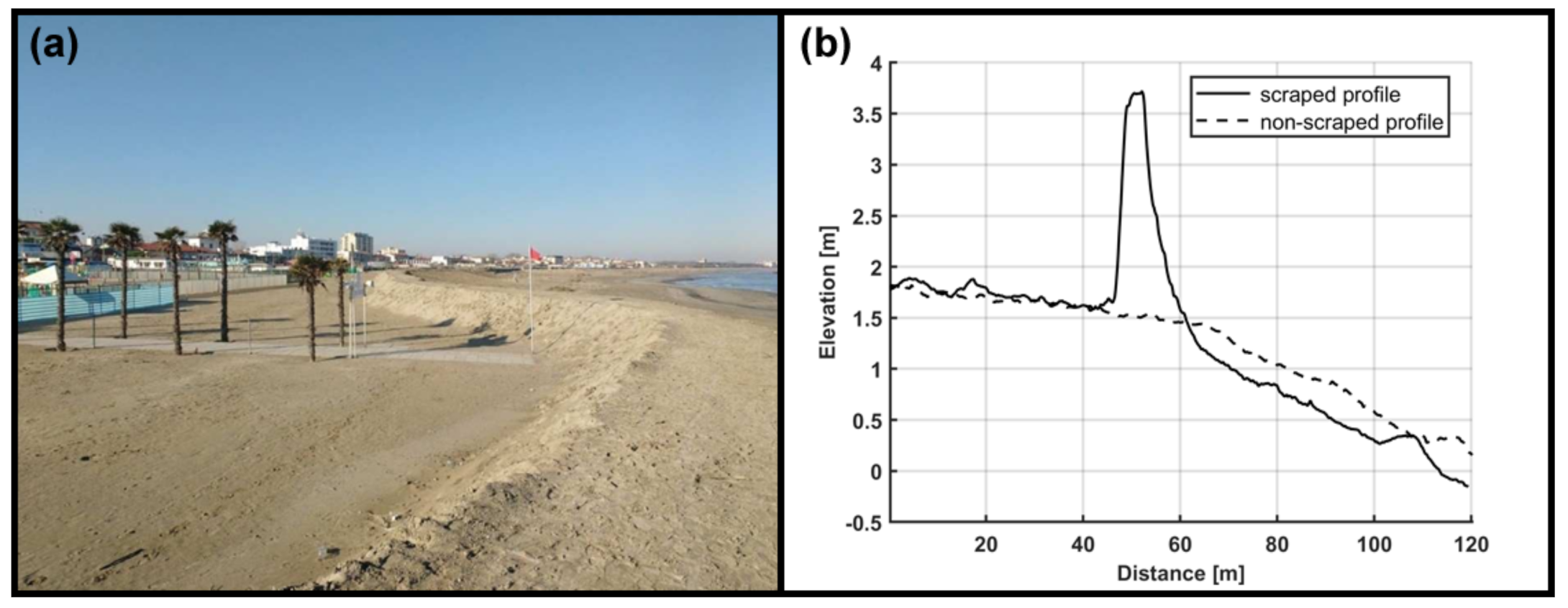
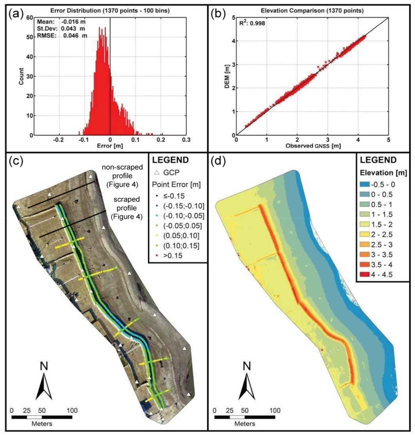
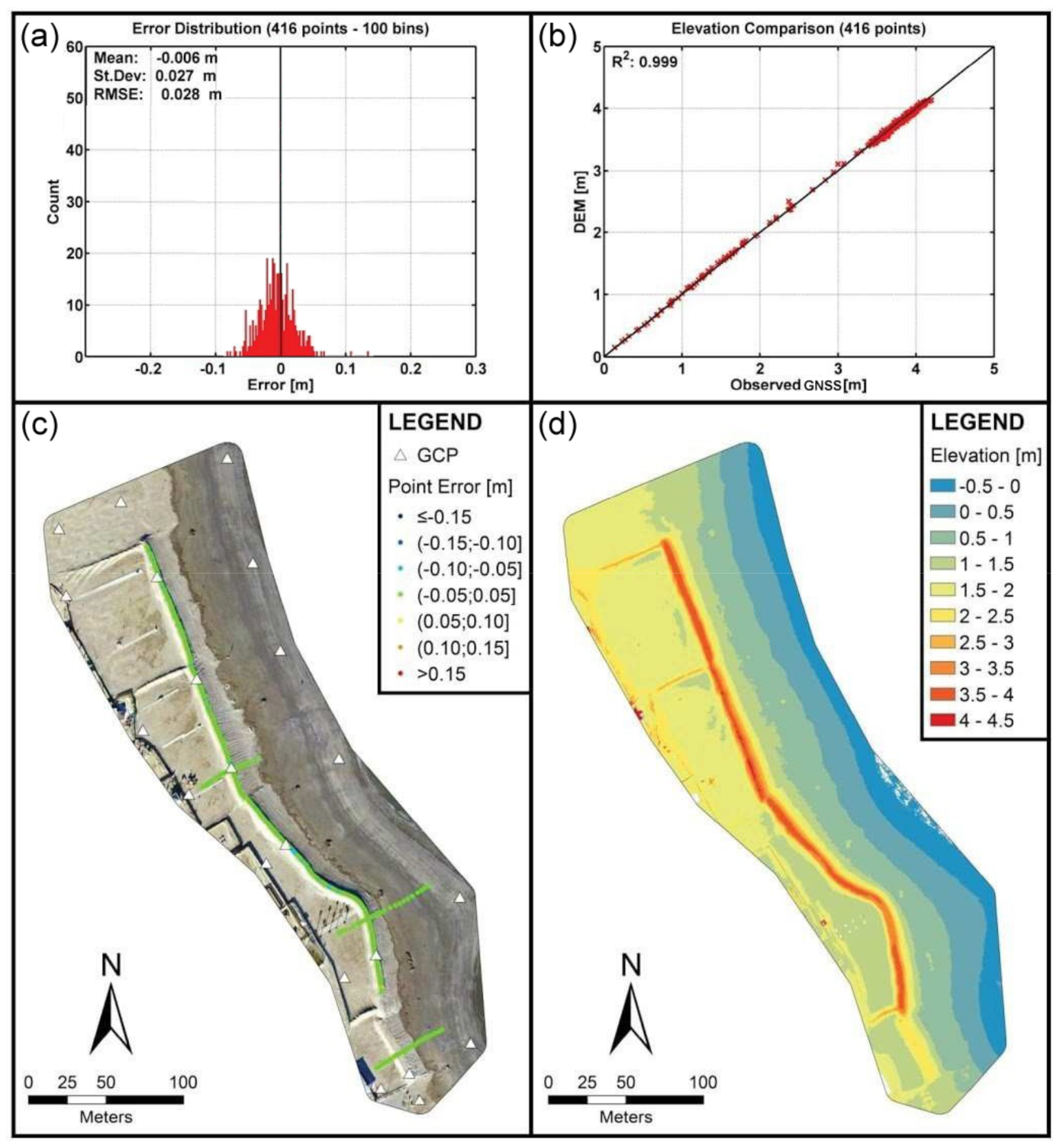
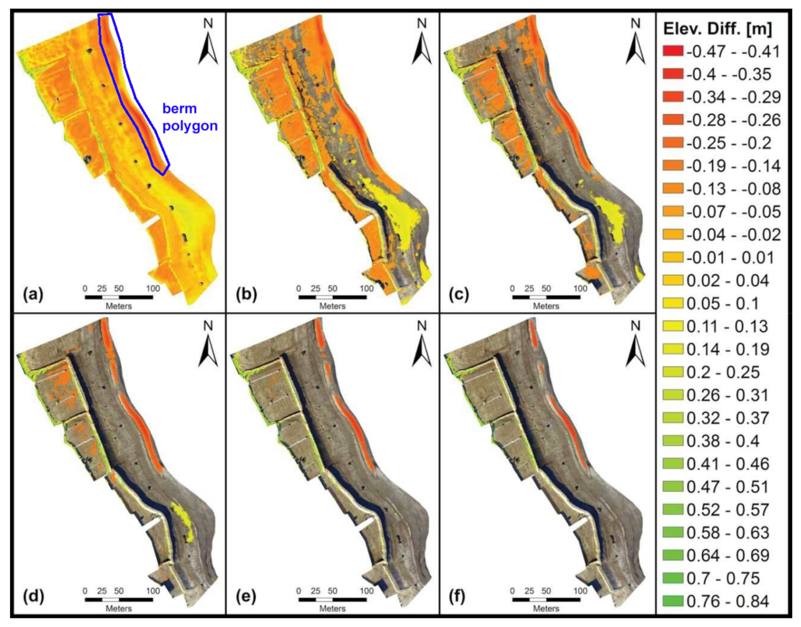
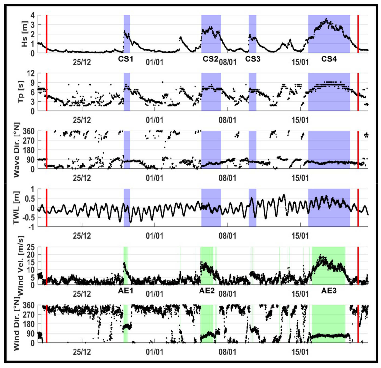
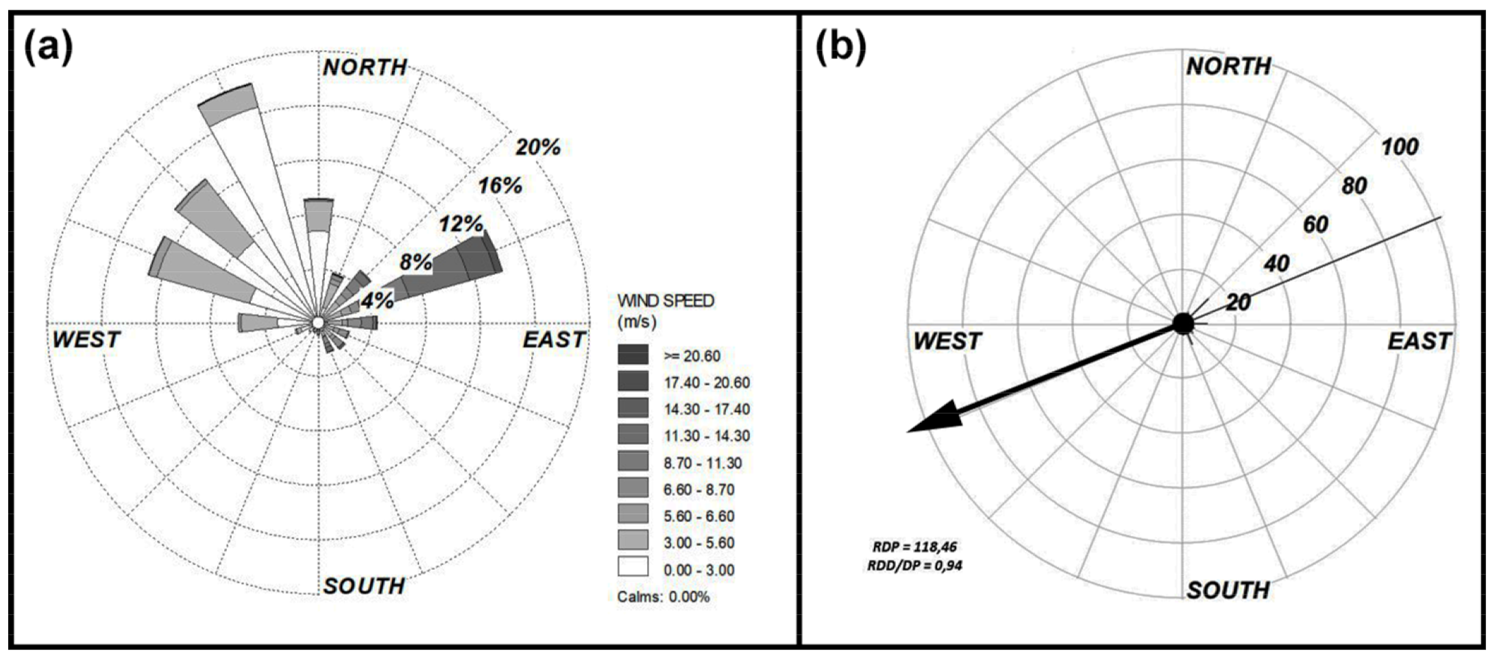
Table 1.
Results of the aeolian transport potential for the identified aeolian events.
| ID | Start | End | RDD 1 | RDP [VU] | RDD/DP |
|---|---|---|---|---|---|
| AE 1 | 28 December 2016 23:40 | 29 December 2016 11:10 | −24 °N (NNW) | 365.6 | 0.985 |
| AE 2 | 5 January 2017 9:20 | 6 January 2017 23:40 | 243 °N (WSW) | 325.2 | 0.958 |
| AE 3 | 16 January 2017 2:00 | 19 January 2017 7:50 | 247 °N (WSW) | 917.7 | 0.995 |
1 Direction the RDP is directed to, in nautical degrees.
Publisher’s Note: MDPI stays neutral with regard to jurisdictional claims in published maps and institutional affiliations. |
© 2021 by the authors. Licensee MDPI, Basel, Switzerland. This article is an open access article distributed under the terms and conditions of the Creative Commons Attribution (CC BY) license (https://creativecommons.org/licenses/by/4.0/).
Share and Cite
MDPI and ACS Style
Duo, E.; Fabbri, S.; Grottoli, E.; Ciavola, P. Uncertainty of Drone-Derived DEMs and Significance of Detected Morphodynamics in Artificially Scraped Dunes. Remote Sens. 2021, 13, 1823. https://0-doi-org.brum.beds.ac.uk/10.3390/rs13091823
AMA Style
Duo E, Fabbri S, Grottoli E, Ciavola P. Uncertainty of Drone-Derived DEMs and Significance of Detected Morphodynamics in Artificially Scraped Dunes. Remote Sensing. 2021; 13(9):1823. https://0-doi-org.brum.beds.ac.uk/10.3390/rs13091823
Chicago/Turabian StyleDuo, Enrico, Stefano Fabbri, Edoardo Grottoli, and Paolo Ciavola. 2021. "Uncertainty of Drone-Derived DEMs and Significance of Detected Morphodynamics in Artificially Scraped Dunes" Remote Sensing 13, no. 9: 1823. https://0-doi-org.brum.beds.ac.uk/10.3390/rs13091823
Note that from the first issue of 2016, this journal uses article numbers instead of page numbers. See further details here.