Article

Hyperspectral Pansharpening in the Reflective Domain with a Second Panchromatic Channel in the SWIR II Spectral Domain

1
Office National d’Études et de Recherches Aérospatiales (ONERA), Département Optique et Techniques Associées (DOTA), Université Fédérale Toulouse, 31055 Toulouse, France
2
Université Paul Sabatier (UPS)-Centre National de la Recherche Scientifique (CNRS)-Observatoire Midi-Pyrénées (UPS)-Centre National d’Études Spatiales (CNES), Institut de Recherche en Astrophysique et Planétologie (IRAP), Université de Toulouse, 31400 Toulouse, France
3
Airbus Defence and Space, 31400 Toulouse, France
*
Author to whom correspondence should be addressed.
Submission received: 7 November 2021 / Revised: 14 December 2021 / Accepted: 23 December 2021 / Published: 28 December 2021

Abstract

:
Hyperspectral pansharpening methods in the reflective domain are limited by the large difference between the visible panchromatic (PAN) and hyperspectral (HS) spectral ranges, which notably leads to poor representation of the SWIR (1.0–2.5 μm) spectral domain. A novel instrument concept is proposed in this study, by introducing a second PAN channel in the SWIR II (2.0–2.5 μm) spectral domain. Two extended fusion methods are proposed to process both PAN channels, namely, Gain-2P and CONDOR-2P: the first one is an extended version of the Brovey transform, whereas the second one adds mixed pixel preprocessing steps to Gain-2P. By following an exhaustive performance-assessment protocol including global, refined, and local numerical analyses supplemented by supervised classification, we evaluated the updated methods on peri-urban and urban datasets. The results confirm the significant contribution of the second PAN channel (up to 45% of improvement for both datasets with the mean normalised gap in the reflective domain and 60% in the SWIR domain only) and reveal a clear advantage for CONDOR-2P (as compared with Gain-2P) regarding the peri-urban dataset.

Graphical Abstract

1. Introduction

Remote-sensing applications for Earth observation, like land-use-map generation [1], vegetation monitoring [2], or classification in urban environments [3,4], need both high spatial and spectral resolutions at local scale, to accurately depict the geometry and state of an observed scene [5,6]. As sensor characteristics are limited [7], hyperspectral pansharpening (or HS pansharpening) methods [8] are used to combine images acquired by two sensor types [9]. On the one hand, panchromatic (PAN) images involve a high spatial resolution but one single broad spectral band almost always included in the (0.4–0.8 μ m) visible (VIS) or (0.4–1.0 μ m) visible and near-infrared (VNIR) spectral domain (for instance: Pléiades [10], EO-1/ALI [11]). On the other hand, hyperspectral (HS) images involve a lower spatial resolution but can contain up to several hundreds of spectral bands, covering, for example, the [0.4–2.5 μ m] reflective domain (for instance: AVIRIS [12], HyMap [13], HySpex [14], EnMAP [15], and EO-1/Hyperion [16]). Note that some imaging systems simultaneously include PAN and HS sensors covering the visible and reflective spectral domains, respectively, like PRISMA [17], HYPXIM [18,19], or EO-1 [20] (ALI + Hyperion).
The various HS pansharpening methods presented in the literature are classified into several main classes, each of them having its own advantages and drawbacks [8]:
  • Component Substitution (CS) methods efficiently preserve the spatial information but cause spectral distorsions [21]. Among the best-suited methods for HS pansharpening, we can cite Gram–Schmidt (GS) adaptive (GSA) [22], Brovey transform (also called Gain) [23,24,25], and Spatially Organized Spectral Unmixing (SOSU) [25].
  • In contrast, MultiResolution Analysis (MRA) methods better preserve spectral information, at the expense of the spatial information [21]. The Modulation Transfer Function-Generalized Laplacian Pyramid (MTF-GLP) [26], MTF-GLP with high pass modulation (MTF-GLP-HPM) [27], and the Optimized Injection Model (OIM) [28], are among the best options among MRA methods for HS pansharpening.
  • To balance the preservation of the spatial and spectral information, hybrid methods aim to compensate the defaults of the previous two classes but need to set more parameters [8]. They include recent methods adapted to HS pansharpening, mostly based on Guided Filters (GF), like GF Pansharpening (GFP) [29,30], Average Filter and GF (AFGF) [31] or Adaptive Weighted Regression and GF (AWRGF) [32].
  • Bayesian and Matrix Factorization (MF) approaches provide high spatial and spectral performance but need prior knowledge about the degradation model, and they imply a higher computation cost [8]. Efficient methods for HS pansharpening are Bayesian Sparse [33,34], a two-step generalisation of Hyperspectral Superresolution (HySure) [35], and a recent variational approach called Spectral Difference Minimization (SDM) [36] for Bayesian approaches as well as Coupled Nonnegative MF (CNMF) [37] and Joint-Criterion Nonnegative MF (JCNMF) [38] for MF approaches.
  • A recently emerged class based on deep-learning (neural-network) supervised models has led to significant advances in image fusion. However, it greatly depends on training data [39]. That is why these methods generally need a large amount of data to provide good performance. Among deep-learning methods adapted to HS pansharpening, one can cite Detailed-based Deep Laplacian PanSharpening (DDLPS) [40], HS Pansharpening with Deep Priors (HPDP) [41], and HS Pansharpening using 3-D Generative Adversarial Networks (HPGAN) [42].
Inprevious work, we selected Gain as the reference method because it fully preserves the information from the PAN image without modifying the spectral information from the HS image. Hence, preprocessing steps have been proposed to extend Gain: they are based on spectral unmixing and spatial reorganisation and aim to refine the information from mixed pixels (pixels whose spectrum is a combination of pure material spectra [43] and which cause most of reconstruction errors). The resulting method is called SOSU [25]. We improved it in several steps [44,45], to efficiently process urban scenes. This led to the Combinatorial Optimisation for 2D ORganisation (CONDOR) method, as proposed in [45].
All HS pansharpening methods suffer from general limitations intrinsic to HS and PAN images including the large gap between the spectral domains covered by these two types of images. This is especially true when the HS image covers the whole reflective domain. In this case, fusion processes can result in spectral distortions in the HS spectral bands outside the PAN spectral domain, which are mostly noticeable beyond 1 μ m . Indeed, as the PAN spectral domain is generally included in the (0.4–0.8 μ m) one, spectral bands from the (0.8–2.5 μ m) spectral domain are insufficiently represented. In our previous work [44,45], this limitation caused poor performance in the (1.0–2.5 μ m) Short-Wave InfraRed (SWIR) spectral domain with the two selected methods, Gain and CONDOR. Furthermore, as the spectral radiance dynamic range is much higher in the (0.4–1.0 μ m) VNIR domain than in the SWIR domain, these fusion methods give much more importance to the former at the expense of the latter.
In addition, an important limitation of HS pansharpening is related to performance-assessment protocols. They are often incomplete as they only evaluate the global quality of fusion processes. Quality criteria are almost always applied to whole images and to the whole HS spectral domain [8]. However, it is crucial to distinguish between the spectral bands of the fused images inside and outside the PAN spectral domain, because the conclusions can largely differ [44], as explained above. Moreover, application of quality criteria is never focussed on specific areas of interest. Nevertheless, it is essential to identify and analyse some particular pixel groups in urban environment (due to the inherent spatial complexity), to provide a more accurate and representative performance assessment. Among these specific pixel groups, there are:
  • Shadowed pixels, which represent a significant proportion of urban scenes, and potential error sources [46];
  • Transition areas, to assess if edges between materials are preserved in fusion results;
  • Pixel groups of varying heterogenity levels, to evaluate methods according to the scene spatial complexity.
Furthermore, local (i.e., pixel-wise) evaluations, like error maps, are rarely proposed in the literature, whereas they are crucial to spatially identify error sources and provide relevant complementary observations [44]. Finally, performance assessments are hardly ever extended to the analysis of the fusion impact on application results (e.g., change detection and classification). Only two studies have analysed the impact of fusion quality on classification, by generating land-cover maps [47,48]. Yet, classification is more adapted to different applications of image fusion that require that the spectral signatures of the fused images correspond to the correct materials.
To overcome these two main limitations, we propose to introduce a second PAN channel associated with the SWIR spectral domain, to supplement the initial PAN channel related to the visible spectral domain. The main objective of this study was to demonstrate the contribution of this innovative instrument concept for HS pansharpening, by selecting the optimal position of the second PAN spectral band in the SWIR domain. To this end, we also propose a complete performance-assessment protocol including refined application of quality criteria (varying pixels groups, pixel-wise local scale) as well as land-use-map generation owing to supervised classification.
This article is structured as follows: In Section 2, CONDOR and Gain are upgraded to efficiently process the two proposed PAN channels, and the complete performance assessment protocol is defined. Then, peri-urban and urban datasets presented in Section 3 are used to assess the two upgraded methods and to compare them with their initial versions (exploiting the visible PAN image only), by performing complete global, refined, and local analyses in Section 4. The contributions and prospects of our work are discussed in Section 5, to conclude on the relevance of the second PAN channel and its implementation in imaging systems.

2. Methodology

In this study, two methods, Gain and CONDOR, presented and compared in previous work [44,45], were extended to process two PAN channels. These new methods are called Gain-2P and CONDOR-2P, respectively. We assumed the following hypotheses:
  • All images are spectral radiances.
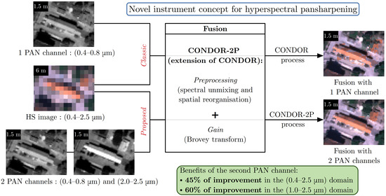
  • The HS image covers the reflective (0.4–2.5 μ m) spectral domain. The two PAN channels are inside the visible domain and the SWIR II (2.0–2.5 μ m) spectral domain, respectively.
  • The HS and PAN images are fully registered, and the HS/PAN spatial resolution ratio, 𝓇, is an integer. Thus, each HS pixel covers the same area as 𝓇 × 𝓇 PAN pixels at this higher spatial resolution. We call these pixels subpixels with respect to the HS data.
Moreover, we considered that each subpixel is pure, which means its spectrum is the spectral signature of one single material. Such a spectrum is called an endmember. However, an HS pixel can be either pure or mixed. In the latter case, we assumed its spectrum is a linear combination of pure material spectra.

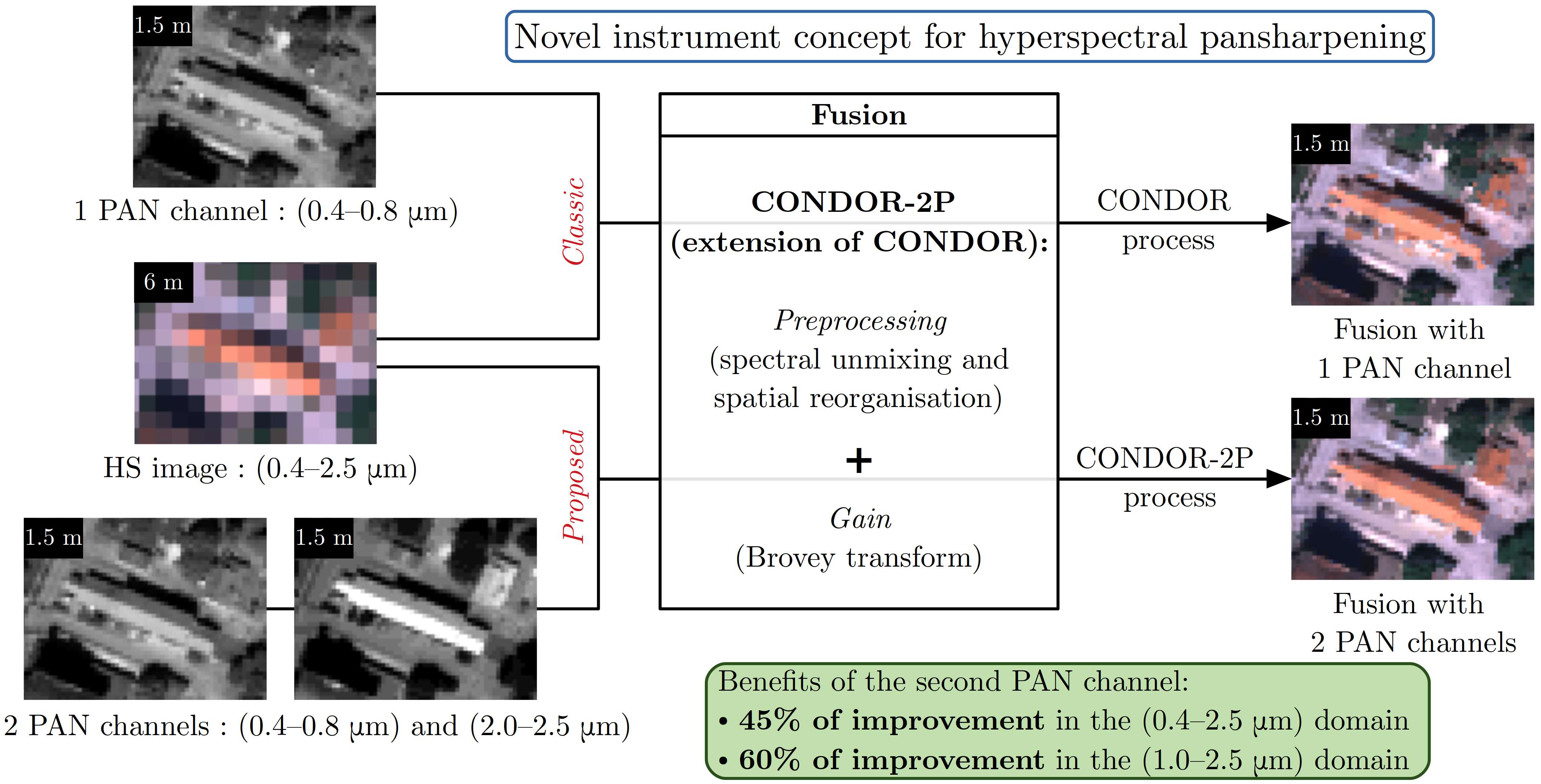
2.1. Description of Gain-2P

H stands for the HS hypercube; P VIS and P SWIR are the two PAN channels covering the visible and SWIR II spectral domains, respectively; and F is the fused hypercube. P ˜ VIS and P ˜ SWIR represent H upsampled (by the nearest-neighbour interpolation) to the the PAN spatial resolution ( H ), which is then integrated in the visible and SWIR II spectral domains, respectively. X ( λ ) stands for the λ th spectral band of an X hypercube. Finaly, the • and     operators represent the term-wise mutliplication and division (Hadamard operators), respectively.
The Gain method, whose principle is recalled in detail in [44], applies a scale factor derived from the PAN image and independent of the spectral band to all pixels of the HS upsampled image. All these scale factors constitute a Gain matrix, whose expression is P VIS P ˜ VIS . Contrary to the initial Gain method, we have two gain matrices, P VIS P ˜ VIS and P SWIR P ˜ SWIR , which means two scale factors to be applied to the spectrum of each subpixel of the upsampled HS image. Thus, we split the reflective domain into two complementary spectral sub-domains, so that we can apply the first scale factor to the sub-domain containing the lower wavelengths ( D 1 ) and the second one to the sub-domain containing the higher wavelengths ( D 2 ), respectively, as depicted in Figure 1. The goal was to determine the most-appropriate limit between D 1 and D 2 (see Section 2.3.1). Therefore, the expression of the fused image is:
F ( λ ) = P VIS P ˜ VIS H ( λ ) if λ D 1 P SWIR P ˜ SWIR H ( λ ) if λ D 2
Like the initial Gain method, the spatial information from the two PAN images was fully injected into the upsampled HS image. In addition, the two PAN images can be restored from the fused image: integrating F over the two PAN spectral domains leads to P VIS et P SWIR .
On the other hand, the spectral information from the upsampled HS image was not altered in the fused image, except at the limit between the D 1 and D 2 application domains. Indeed, if the two scale factors differ, they will provide a discontinuity between the two associated parts of the processed spectrum. To limit the effects of any discontinuity, we chose a transition wavelength in an atmospheric absorption band, because the associated spectral bands are non-exploitable (owing to low atmospheric transmission), and thus they are not retained (see Section 3.1.1).

2.2. Description of CONDOR-2P

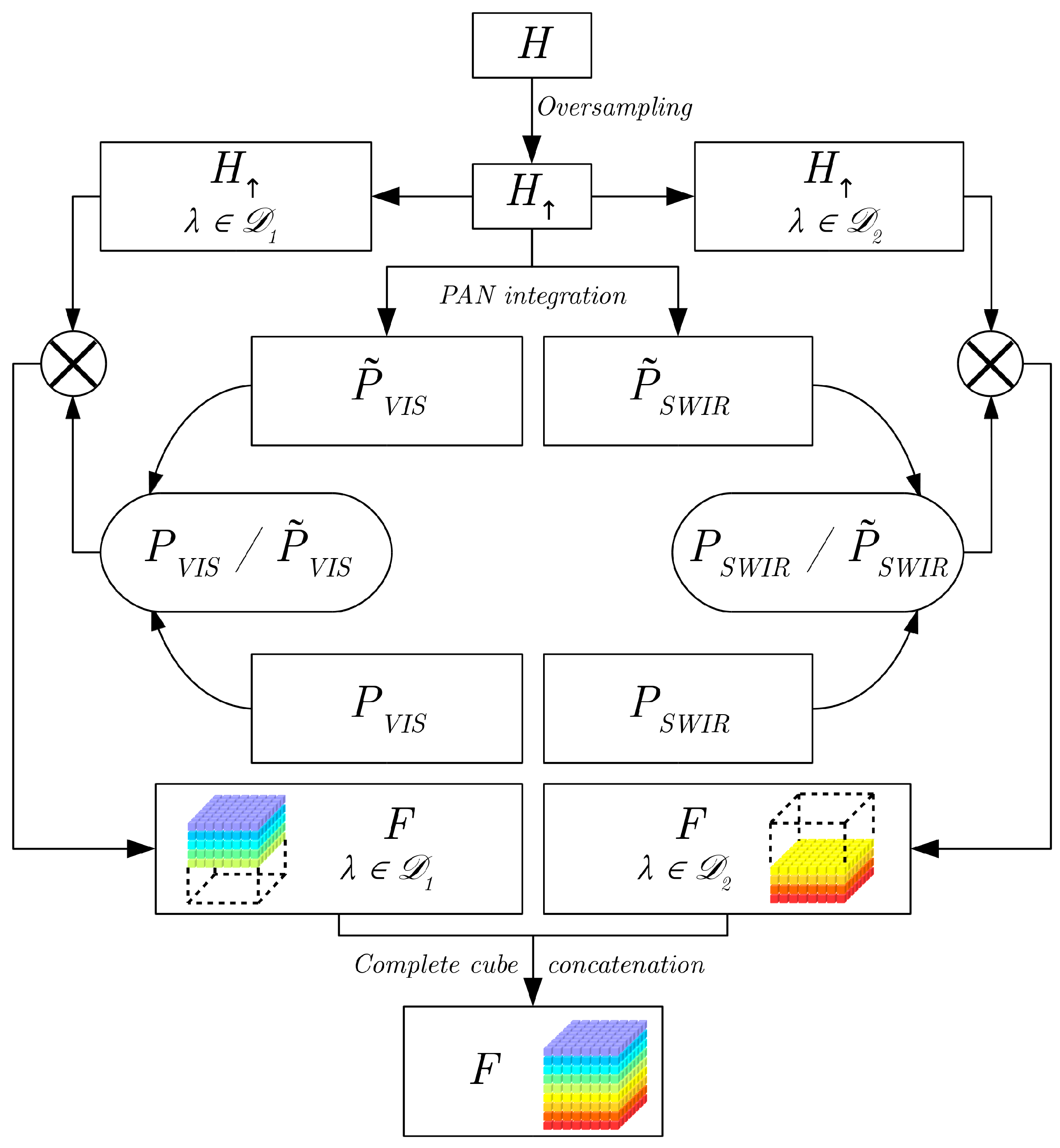
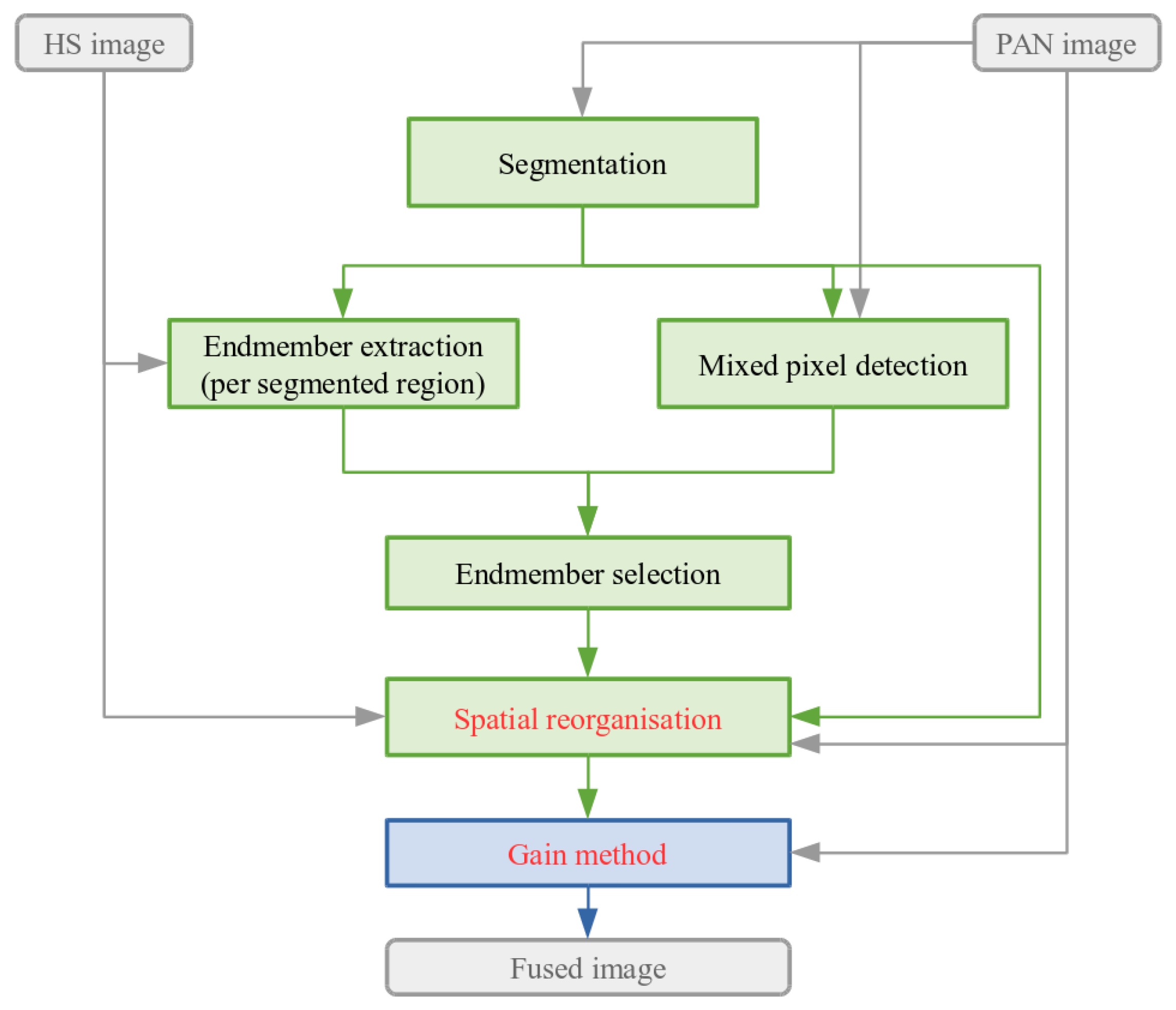
2.2.1. CONDOR Principle

CONDOR is based on the Gain method but adds preprocessing steps to detect mixed pixels and refine their spatial and spectral information. It includes six main steps (Figure 2), described in detail in [44], and it has been recently improved to reduce the computation time in [45]. The first five steps constitute CONDOR preprocessing, whereas the last one is the fusion process:
  • The segmentation step splits the high-spatial-resolution PAN image into several regions with low spectral variability.
  • Separately for each segmented region consisting of a set of HS pixels, the endmember extraction step aims to estimate the associated endmembers.
  • The mixed pixel detection step identifies the mixed HS pixels by referring to the segmentation map (step 1).
  • For each mixed HS pixel (step 3), the endmember selection step gathers a list of possible endmembers depending on the corresponding segmented regions (steps 1 and 2) and the neighbouring pure pixels.
  • For each mixed HS pixel, the spatial reorganisation step assigns the right endmembers to the right subpixels (following hypothesis 4 in the introduction of Section 2), to preserve as much as possible the spatial and spectral information of the PAN and HS images.
  • The Gain process applies a scale factor derived from the PAN image and independent of the spectral band to all pixels of the reorganised image.
The most-important step is spatial reorganisation (step 5). This step performs a combinatorial analysis of every possible combination of pairs constituted of one segmented region present in the mixed HS pixel (step 1) and one potential endmember (step 4). For each tested combination, we generated the corresponding spatial reorganisation by assigning the chosen endmembers to all the subpixels of the paired regions, as shown in Figure 3.
Then, the best spatial reorganisation is the one minimizing a cost function based on two criteria (PAN and HS reconstruction errors). To reduce the computation time, this combinatorial analysis was modelled in [45] as a Mixed Integer Linear Programming (MILP) optimisation problem, and adapted solvers were used.

2.2.2. CONDOR-2P: Method Description

Previous work proved that the HS criterion of CONDOR is inaccurate for complex area processing like urban areas [45]. Indeed, it does not take into account the location of the subpixels and can lead to incoherent spatial reorganisation. In addition, the PAN criterion, although much more accurate, is not always sufficient by itself to deduce the best spatial reorganisation, or, at least, to lead to a correct reconstruction. In particular, the PAN criterion does not take the SWIR spectral domain into account. Therefore, with the help of the second PAN channel, we chose to replace the HS criterion by a second PAN criterion, better taking the SWIR spectral domain into account.
Thus, we developed CONDOR-2P by modifying:
  • The spatial reorganisation step (step 5), to minimize a cost function composed of two PAN criteria (Section 2.2.3);
  • The fusion process (step 6), by using Gain-2P (Section 2.1).
The other steps of this method remain unchanged.

2.2.3. CONDOR-2P: Spatial Reorganisation Improvement

Defining the PAN Reconstruction Errors

The selected reorganisation is the one minimizing a cost function based on two reconstruction errors derived from the PAN channels in the visible and SWIR II spectral domains called E PAN VIS and E PAN SWIR , respectively.
Contrary to previous work [45] for which the 1-norm was selected, we here chose to define E PAN VIS and E PAN SWIR by using the (Euclidean) 2-norm. The argument for this choice is that PAN reconstruction errors expressed with the 2-norm can be simplified as linear functions of the variables to be optimized, as shown in this section. However, this is not possible with the 1-norm, because of the absolute-value operator. Note that the 1-norm was necessary in previous work because the HS criterion cannot be simplified with the 2-norm.
Therefore, E PAN VIS and E PAN SWIR are defined as normalised RMSE (NRMSE). To ensure a compatible numerator and denominator (second-order norms), we did not merely normalise by the mean ( mean [ X ] ) or the range ( max [ X ] min [ X ] ) of the X reference data but by mean [ X 2 ] . The entire expression of the NRMSE is therefore contained in a square root. The latter is removed, because, as a strictly increasing function in R + , it has no impact on the minimization of the associated error. Thus, we get the Normalised Mean Square Errors (NMSE) expressed as:
E PAN VIS = mean j P VIS j mean λ ( R j , λ ) 2 mean j P VIS j 2 = j P VIS j 1 n λ · λ ( R j , λ ) 2 j P VIS j 2 E PAN SWIR = mean j P SWIR j mean λ ( R j , λ ) 2 mean j P SWIR j 2 = j P SWIR j 1 n λ · λ ( R j , λ ) 2 j P SWIR j 2
where j, λ , and λ are indices parsing the 𝓇 × 𝓇 associated subpixels, the n λ spectral bands included in the visible spectral domain, and the n λ spectral bands included in the SWIR II spectral domain, respectively. P VIS j and P SWIR j stand for the spectral-radiance values of the j th corresponding subpixel of the PAN image in the visible and SWIR II spectral domain, respectively; R j , λ represents the spectral radiance value of the λ th spectral band of the j th subpixel in the spatial reorganisation to be tested.
We showed in [45] that R j , λ can be expressed in terms of combinatorial choices:
R j , λ ( 𝟙 k , r ) = k e k , λ · r 𝟙 k , r · 𝟙 j , r
where k and r are indices parsing the list of all the potential endmembers and all the segmented regions in the processed mixed pixel, respectively; 𝟙 k , r is a Boolean variable equal to 1 if and only if the k th endmember is assigned to the r th region; and 𝟙 j , r is a Boolean independent of the tested spatial reorganisation, equal to 1 if and only if the j th subpixel is localised in the r th region.

Properties

To simplify the expressions of E PAN VIS and E PAN SWIR , three properties were used in the following:
  • P-1 One and only one endmember is assigned to each region, i.e.,:
    k 𝟙 k , r = 1 r
  • P-2 Each subpixel belongs to one and only one region, i.e.,:
    k 𝟙 j , r = 1 j
  • P-3  The Boolean 𝟙 k , r and 𝟙 j , r terms verify:
    𝟙 k , r 2 = 𝟙 k , r 𝟙 j , r 2 = 𝟙 j , r

Development of the PAN Reconstruction Errors

The development presented in this section is valid for both E PAN VIS and E PAN SWIR . Let E PAN be one of these reconstruction errors, and let λ be the index parsing the integration domain of the associated PAN channel. By injecting the expression of R j , λ ( 𝟙 k , r ) (see (3)) into (2) and taking into account the properties previously defined, we simplified the developed expression of E PAN . Thus, minimizing E PAN is equivalent to minimizing the following f PAN ( 𝟙 k , r ) function:
f PAN ( 𝟙 k , r ) = k , r 1 j P j 2 · j e k ¯ 2 2 P j e k ¯ 𝟙 j , r · 𝟙 k , r
where e k ¯ is the mean of the e k endmember in the considered PAN spectral domain:
e k ¯ = 1 n λ · λ e k , λ
Thus, f PAN ( 𝟙 k , r ) can be summed up as:
f PAN ( x i ) = i C i · x i
with:
i = ( k , r ) ( index parsing n k × n r elements ) C i = C k , r = j e k ¯ 2 2 P j e k ¯ 𝟙 j , r j P j 2 x i = 𝟙 k , r
where n k and n r stand for the number of available endmembers and the number of regions associated with the processed mixed HS pixel, respectively.

Modelling the Whole Optimisation Problem

The total cost function to be minimized, f PAN ( 𝟙 k , r ) , is expressed as a linear combination of the intermediate f PAN VIS and f PAN SWIR cost functions, where C VIS k , r and C SWIR k , r are their associated C k , r coefficients (see (10)):
f PAN ( 𝟙 k , r ) = α · f PAN SWIR ( 𝟙 k , r ) + ( 1 α ) · f PAN VIS ( 𝟙 k , r ) = k , r α · C SWIR k , r + ( 1 α ) · C VIS k , r · 𝟙 k , r = k , r C total k , r · 𝟙 k , r
The α weight, defined on the [ 0 , 1 ] interval, is a configurable parameter that can be used to control the relative influences of both f PAN VIS and f PAN SWIR . α values from 0 to 1 in steps of 0.1 were tested, and 0.5 provided optimal results. In addition, α = 0.5 gives the same importance to both PAN channels (because of normalisation). For these reasons, α was fixed to 0.5 . Therefore, we get the following MILP optimisation problem:
minimize f PAN ( 𝟙 k , r ) = k , r C total k , r · 𝟙 k , r such that k 𝟙 k , r = 1 , r and 𝟙 k , r { 0 ; 1 } n k · n r
An optimal solution to this MILP problem can be systematically found by the CBC solver [49]. The latter was also selected because it is less time-consuming than other reliable tested solvers, like GLPK [50].

2.3. Selected Spectral Domains

Following the descriptions of Gain-2P and CONDOR-2P, two parameters had to be chosen: the spectral domain used to generate the second PAN channel (Section 2.3.1) and the application domains of Gain-2P (Section 2.3.2).

2.3.1. SWIR Band Selection

Concerning the second PAN image, we chose to focus on the SWIR II spectral domain (2.0–2.5 μ m), because it contains the spectral bands furthest from the visible domain, in the reflective range. This way, we retrieved the most complementary and exhaustive information from the two PAN channels. To this end, three spectral intervals related to the SWIR II domain were tested. The first one is the whole SWIR II domain, which is unrepresentative of the current instrumental constraints, whereas the two other ones were obtained by checking the spectral ranges acquired by the existing MultiSpectral (MS) imaging systems. Thus, the considered spectral intervals are:
  • The whole (2.0–2.5 μ m) SWIR II spectral interval, partially identified in brown in Figure 4;
  • The (2.025–2.35 μ m) spectral interval, identified in green in Figure 4, corresponding to the SWIR II spectral band of Sentinel-2 [51] (more precisely: (2.027–2.377 μ m) for S2A and (2.001–2.371 μ m) for S2B). It also corresponds to the HS spectral range retained in the SWIR II domain after removing the non-exploitable HS spectral bands (see Section 3.1.1) for the three tested datasets, as shown in Figure 4;
  • The (2.2–2.3 μ m) spectral interval, identified in orange in Figure 4, corresponding to the SWIR II spectral band of Sentinel-3 [52] (more precisely: (2.206–2.306 μ m) for SLSTR and (2.2–2.3 μ m) for Synergy).
A sensitivity study is performed in Section 4.1 to determine the most-adapted spectral interval among the three proposed ones.

2.3.2. Gain-2P Limit Selection

Adapted limits between the D 1 and D 2 application domains of Gain-2P had to be determined before performing complete analyses. Note that Gain-2P was also used as the fusion step of CONDOR-2P; thus, the limit will affect both fusion methods. As explained in Section 2.1, each analysed tested limit must be located in an atmospheric absorption window. Nevertheless, the exact location of a limit within a single atmospheric absorption window does not matter. Therefore, there is a limited number of possible choices. Thus, we identified three limits, each of them corresponding to a different atmospheric absorption band, as depicted in Figure 4:
  • 0.95 μ m ;
  • 1.15 μ m ;
  • 1.35 μ m .
However, we only retained the 0.95 μ m and 1.35 μ m limits. Indeed, the 1.15 μ m limit systematically provides intermediate results as compared with the results obtained with the other two limits. The associated sensitivity study is performed in Section 4.2.

2.4. Performance-Assessment Protocol

2.4.1. Wald’s Protocol and Quality Criteria

Generating simulated PAN and HS images by degrading a single reference HS image having a high spatial resolution (called the REF image) allows the use of Wald’s protocol [53]: the fusion method quality is quantified by comparing the fused and the REF images. To this end, four common quality criteria from the literature were used, each of them evaluating the spatial, spectral, or global quality of the fusion result: Spectral Angle Mapper (SAM, spectral), Cross-Correlation (CC, spatial), Root Mean Square Error (RMSE, global), and Erreur Relative Globale Adimensionnelle de Synthèse (ERGAS, global). They are complementary and among the most-reliable quality criteria [54].
These four literature criteria were supplemented by a simple criterion called Mean Normalised Gap (MNG, global). It consists in calculating a normalised error (1-norm) between the REF and fused images, noted Normalised Gap (NG), for each element of the hypercube (i.e., pixel-wise and band-wise). The MNG, expressed in percent, is the mean of the NG of all the pixels and the spectral bands. Its expression is given in (13), where X ^ is the estimated fused image and X is the REF image:
MNG ( X ^ , X ) = mean | X ^ X | X
In Section 4, we also focus on several single spectral bands: NG values are calculated for each element of the associated 2D matrices, so that the error distribution of the chosen spectral bands can be analysed (as detailed in Section 2.4.3).
To get a robust exhaustive performance-assessment protocol, the five quality criteria can be applied to different spectral domains: VNIR, SWIR, and reflective (VNIR-SWIR). Spatially, they can be applied to:
  • The whole images (global analysis);
  • Various spatial regions (refined analysis): pixel groups built according to specific similarities (transition zones, shadowed areas, pixels of similar variance ranges, as described in Section 2.4.2);
  • Each pixel of the scene (local analysis) for the global and spectral criteria: this evaluation is used to analyse the spatial variation of the error (Section 2.4.3).
This leads to a refined quality protocol.

2.4.2. Refined Analysis: Pixel Group Location

Transition Areas

Pixels corresponding to spatial transitions are identified by performing two complementary variation tests:
  • The first test focuses on spectral-radiance variations and is useful to detect an irradiance change for one single material. It is applied to the PAN image, and is based on the Canny edge detector [55], except that a simple threshold is used to identify the pixels associated with transitions (to ensure thick edges and thus complete transitions): a pixel is regarded as part of transition if and only if the corresponding value in the edge-detection map is superior to the mean value of this map.
  • The second test aims to identify distinct materials, even if their spectral radiances in the PAN image are similar. It is applied to the REF image (high-spatial-resolution HS image, see Section 3.1) and computes, for each pixel, the SAM between its spectrum and the ones of the four closest neighbouring pixels (left, right, top, and bottom), to deduce a single summed SAM value. A pixel is regarded as part of transition if and only if the corresponding value of the SAM variation map is superior to a fixed threshold. Here, a threshold of 1.5 times the averaged value of the SAM variation map was empirically set. Then, to ensure thick edges (and thus complete transitions), we applied two morphological operations to this mask: the first one removing isolated points, followed by a dilatation.
Each pixel is counted up as being part of a transition area if a variation is detected by at least one of the two tests.

Shadowed and Sunlit Pixels

To detect shadowed pixels, we applied the following I spectral index from the literature [56] to the REF image:
I = 1 6 · 2 R R + R G + R B + 2 R NIR
where R R , R G , R B , and R NIR stand for the REF image restricted to the averaged spectral band of the red, green, blue, and Near-Infrared (NIR) spectral domains, respectivey. The obtained shadow spatial mask is then thresholded, by choosing the adapted value for each dataset. The pixels that are not detected as shadowed automatically count as sunlit.

Variance Ranges

To assess the method performance according to the spatial complexity of the scene, a variance map is generated at the spatial resolution of the HS image used as input for the fusion methods. For each HS pixel, we refer to the group of subpixels covering the same area in the PAN image, and we calculated the variance [57] of the associated spectral radiance values in the PAN image. Then, each HS pixel of the scene was ranked according to its variance value, to generate masks corresponding to the following variance ranges (in W 2 ·m 4 ·sr 2 · μ m 2 ): [ 0 ; 5 ] , [ 5 ; 10 ] , [ 10 ; 15 ] , and [ 15 ; + ] . Finally, these masks were upsampled (by nearest-neighbour interpolation) to the higher PAN spatial resolution.

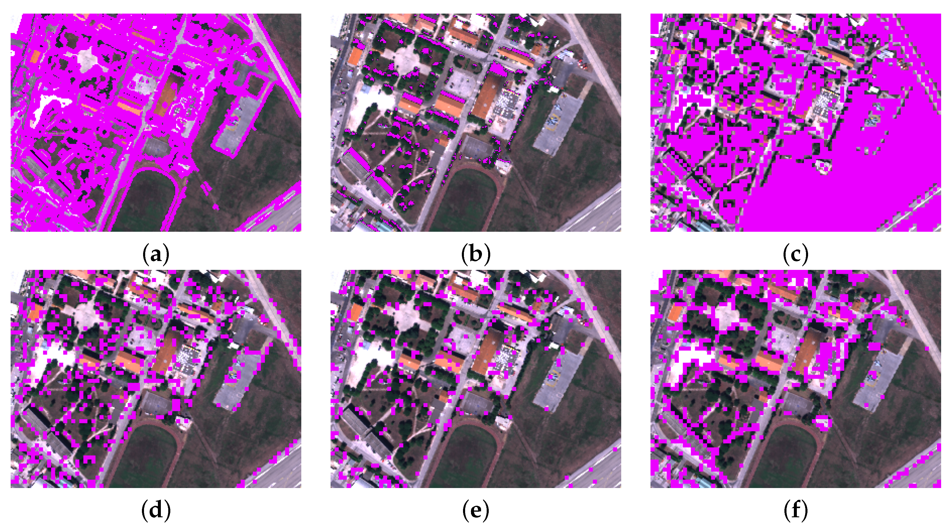
2.4.3. Local Analysis: Spatial Error Variation

For each spectral band, one can pixel-wisely apply any global quality criterion to the corresponding 2D-image representing this spectral band. It is then possible to examine the spatial distribution of the chosen quality criterion on the considered spectral bands, by generating a box plot [58]. In Section 4.2.3, we use the NG (see Section 2.4.1) to generate these box plots. We notably focus on outliers provided by these charts, to locally assess the reconstruction errors.

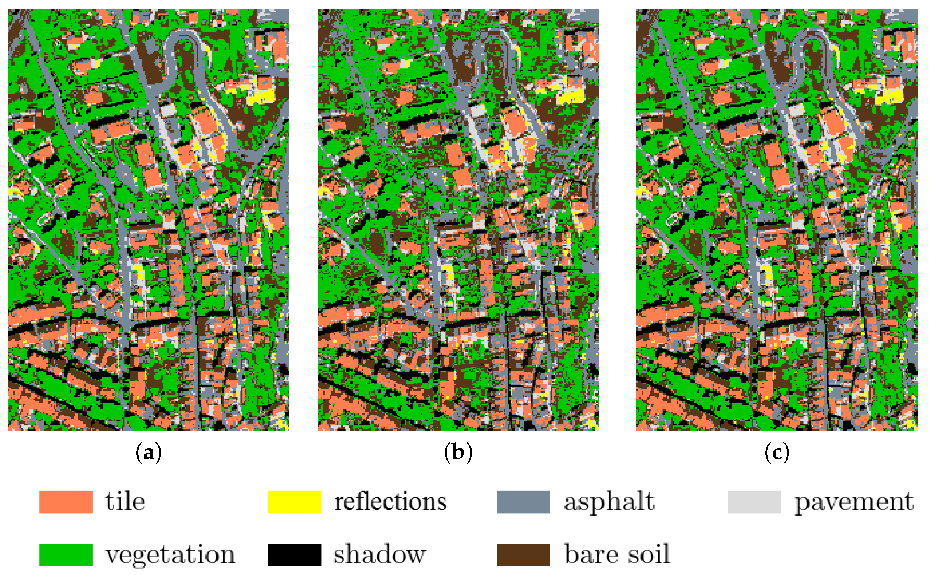
2.4.4. Generation of the Classification Map

To supplement the presented performance assessment protocol, classification maps were computed by using supervised classification. This way, one can assess the fusion impact on classification, by checking if each pixel is assigned to the right class.

Supervised Classification: Training and Validation of the Model

We opted for a supervised classification based on machine learning, largely used to provide cartography in various applications [59]. In the analysed scene, we identified n classes of materials. For each of these classes, 20 representative spectra were collected in the REF image to train and validate the model. We applied the commonly used random forest classifier [60] and performed a cross validation [61] called stratified k-fold [62], with five successive repetitions. We defined the model accuracy [63] as the average percentage of well-classified spectra (i.e., assigned to the correct class) from the training dataset.

Land-Cover Maps

The trained model was applied to the spectra of all the pixels of the REF and fused images, to obtain land-cover (or classification) maps (each pixel assigned to a class) before and after fusion processes. The classification map related to the REF image was considered as the reference classification map. Therefore, by comparing this reference classification map with the one of a fused image, one can deduce the percentage of concordant pixels (i.e., assigned to the same class in both classification maps). This overall accuracy [63] can be computed for the different pixel groups described in Section 2.4.2.

3. Datasets

3.1. Image Simulation

Each dataset used to apply and compare fusion methods contains an REF image (HS image), and simulated images were obtained by degrading the REF image (to apply Wald’s protocol—see Section 2.4.1): one HS image with lower spatial resolution and two PAN images. All HS images are represented by the following colour composite images in this article: red, green, blue (RGB) for the visible domain and 1.25 , 1.65 and 2.20 μ m for the SWIR spectral domain.

3.1.1. REF Image

Each REF image was extracted from an airborne flight line HS image acquired in the reflective domain (0.4–2.5 μ m) with the HySpex Odin (FFI/NEO) instrument from the SYSIPHE imaging system (ONERA) [64] during the 2015 Canjuers airborne campaign [65]. The spatial resolution of these airborne images was 0.5 m, but the REF images were downsampled to 1.5 m spatial resolution. The downsampling process corresponds to a spatial averaging of 3 × 3 pixels. Additionally, the REF images were obtained by removing the spectral bands whose wavelengths corresponded to an atmospheric transmission coefficient lower than 0.8 , which led to 248 final spectral bands, out of the 426 initially available ones.

3.1.2. HS Image

The HS image was obtained by spatially averaging the REF image, by the 𝓇 spatial resolution ratio. Here, a value of 4 was used.

3.1.3. PAN Images

Both visible and SWIR PAN images were obtained by spectrally averaging the REF image. This consists in uniformly aggregating all the spectral bands of the REF image included in the appropriate spectral domain (visible or chosen spectral interval in the SWIR II domain). The spatial resolution of the generated PAN images is the same as the REF image one.

3.2. Dataset Description

Three datasets were used to test and compare the fusion methods:
  • Peri-urban dataset (“stadium”, Figure 5): The extracted REF image represents a part of a sports complex from Canjuers (France). It covers a small scene ( 64 × 64 pixels), which includes a stadium, buildings, and vegetation. This dataset was used to test different spectral intervals for the second PAN channel, before performing complete analyses with the following two datasets.
  • Peri-urban dataset (“Toulon”, Figure 6): The extracted REF image covers a part of the airport of Toulon-Hyères (France). This image, which contains 288 × 216 pixels, is larger and more complex than “Stadium” as it includes buildings, natural (fields, wastelands, trees, and a park) and man-made (roads, car and aircraft parking areas, and a landing strip) soils, a stadium, and very reflective structures (greenhouses and cars).
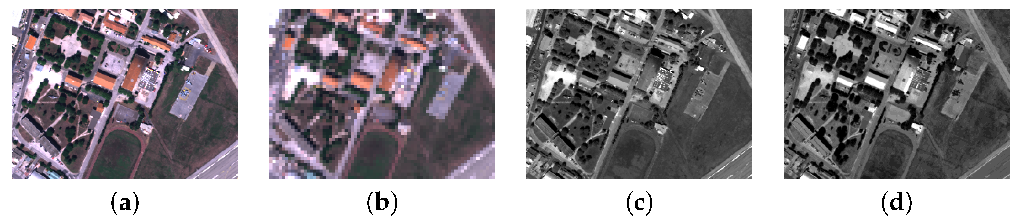
  • Urban dataset (“Gardanne”, Figure 7): The extracted REF image represents a part of Gardanne (France). It contains 192 × 288 pixels and covers residential areas (suburbs with spaced houses and gardens) and a compact city centre.

4. Results

This section is composed of four subsections corresponding to the following steps:
  • Section 4.1: selecting the optimal SWIR band by testing the three intervals defined in Section 2.3.1;
  • Section 4.2: selecting the optimal Gain-2P limit, by testing the two values defined in Section 2.3.2;
  • Section 4.3: comparing the fusion methods using one PAN channel with their extended versions using two PAN channels, to demonstrate the benefit of this instrument concept;
  • Section 4.4: comparing CONDOR-2P with Gain-2P, to determine the most appropriate method in the case of two PAN channels.
The first step was performed by using the small “Stadium” peri-urban dataset. The results corresponding to the last three steps were simultaneously obtained with the two extended datasets: “Toulon” (peri-urban) and “Gardanne” (urban).
The parameters of CONDOR and CONDOR-2P are:
  • Segmentation method: over-segmentation (described and justified in [44]) based on the Meanshift [66] classifier, with quantile  = 0.1 and samples = 30 (“Stadium” and “Gardanne”) or 40 (“Toulon”);
  • Number of endmembers extracted per region: 2;
  • Pure pixel selection neighbourhood: 2;
  • Weighting of cost functions for the spatial reorganisation optimisation problem: α = 0 for CONDOR (PAN criterion only, no HS criterion), α = 0.5 for CONDOR-2P (see Section 2.2.3).

4.1. Sensitivity Study: SWIR Band of the Second PAN Image

To identify the optimal SWIR band, Gain-2P and CONDOR-2P were applied to the “Stadium” peri-urban dataset for three configurations. Each of them corresponds to one of the spectral intervals proposed in Section 2.3.1 to generate the second PAN channel: (2.0–2.5 μ m), (2.025–2.35 μ m), and (2.2–2.3 μ m). We chose the 0.95 μ m limit between D 1 and D 2 (defined in Section 2.1), among the three wavelengths selected in Section 2.3.2, because it corresponds to the separation between the VNIR and SWIR spectral domains. The associated numerical results are displayed in Table 1.
These values were very close for all three proposed domains, both with Gain-2P and CONDOR-2P. Nevertheless, in the reflective domain, there was a slight advantage for the (2.025–2.35 μ m) spectral domain with CONDOR-2P, notably for RMSE and ERGAS (up to 0.8 % of improvement for RMSE). In contrast, the slight advantage was for the (2.2–2.3 μ m) spectral domain with Gain-2P, notably for SAM, RMSE, and ERGAS (up to 0.6% of improvement for ERGAS). Therefore, all three tested intervals led to close numerical results. Hence, the choice of the optimal interval was based on three criteria: best performance, highest spectral radiance, and highest atmospheric transmission. The best trade-off was obtained with the (2.025–2.35 μ m) interval. The latter was thus retained to systematically generate the second PAN channel.
Concerning quality criteria, the CC values were too close to 1 and too close to each other to provide meaningful conclusions. Concerning the global measures, ERGAS does not provide any additional information as compared with RMSE. These two observations were also confirmed by the numerical results obtained with the “Toulon” and “Gardanne” datasets. Therefore, we only focused on MNG, SAM, and RMSE in Section 4.2, Section 4.3 and Section 4.4.

4.2. Sensitivity Study: Gain-2P Limit

Two extended datasets are analysed in Section 4.2, Section 4.3 and Section 4.4: a peri-urban dataset (“Toulon”) and an urban one (“Gardanne”).
As explained in Section 2.3.2, choosing a limit between the two application domains of Gain-2P also affects CONDOR-2P. Indeed, the former is the fusion step of the latter (see Section 2.2.2). That is why both Gain-2P and CONDOR-2P results are discussed to select the optimal limit.

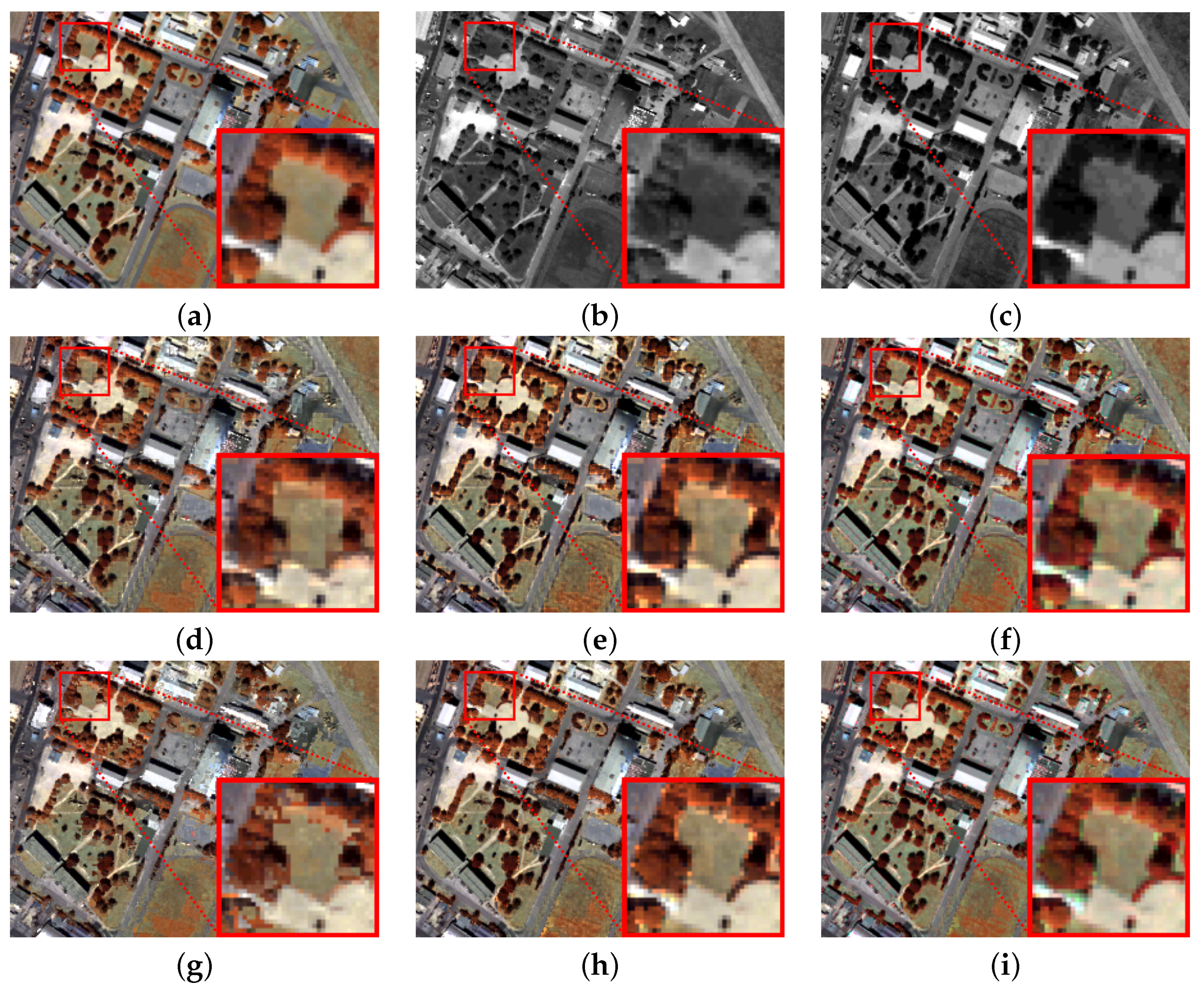
4.2.1. Visual Analysis

Global visual results are shown in Figure 8 for the peri-urban dataset, for which the differences are more significant. These results were obtained with all four tested fusion methods (with 0.95 μ m and 1.35 μ m limits, see Section 2.3.2), by the SWIR colour composite (see Section 3.1). The RGB colour composite is not provided because the visual results would be the same for Gain and Gain-2P with both limits, as well as for CONDOR-2P with both limits. Indeed, these spectral bands are systematically associated with the scale factor from the visible PAN image by Gain and Gain-2P.
The two limits cause different types of distorsions, for both Gain-2P and CONDOR-2P:
  • Isolated artefacts, for example, on the tree edges (see red frame in Figure 8), with the 0.95 μ m limit;
  • Spectral distortions (colours non-representative of the REF image) with the 1.35 μ m limit. These spectral distorsions are due to the fact that the scale factor is not the same for all three displayed spectral bands ( 1.25 , 1.65 and 2.20 μ m ) with the 1.35 μ m limit, contrary to the 0.95 μ m one. Therefore, this degradation only depends on representation choices.
Nevertheless, these degradations are visually more reduced with the 1.35 μ m limit. Therefore, choosing this latter limit seems to be visually the best choice.

4.2.2. Global and Refined Analyses

Table 2 and Table 3 show the global and refined numerical results of the fusion methods applied to both datasets calculated for the whole images and the transition areas, respectively. The latter represent 50 % of the scene in the peri-urban case and 62 % in the urban case.
The methods systematically provide better performance when the quality criteria are applied to the whole images than when they are applied to the transition areas. Furthermore, numerical results between these two pixel groups only differ by a constant scale factor. In other words, the relative performance of the fusion methods remained similar. These two observations can be explained by the fact that, for both pixel groups, reconstruction errors mostly come from transition areas. Thus, conclusions established from these numerical results are valid for the whole images as well as the transition areas.
In the peri-urban case, the numerical results confirmed that the 1.35 μ m limit improves the performance of CONDOR-2P and Gain-2P as compared with the 0.95 μ m one (see underlined values). Although the 1.35 μ m limit choice has little influence on the VNIR spectral domain, it enhances results in the SWIR spectral domain (notably, for both methods: an improvement rate of about 22 % for the MNG criterion and RMSE values almost divided by two), which therefore enhances results in the whole reflective domain (notably, for both methods: an improvement rate of about 12 % for the MNG criterion). The SAM is an exception because the associated values in the SWIR spectral domain are lower with the 0.95 μ m limit than with the 1.35 μ m one. This can be explained by the fact that, with this latter limit, the scale factor applied to the spectral bands is not the same over the whole SWIR spectral domain, which causes a degradation in terms of spectral shape. Nevertheless, this degradation is relatively weak (no more than a 0 . 3 gap as compared with the 0.95 μ m limit). Thus, this gap is insufficient to produce better SAM values in the whole reflective range with the 0.95 μ m limit.
In the urban case, the methods provide closer performance with the two limits. Yet, numerical results obtained with the 1.35 μ m limit remain superior for the whole set of quality criteria applied to the reflective and VNIR domains. For the SWIR domain, only the SAM criterion provides better results with the 0.95 μ m limit ( 10 % gap for both methods). As in the peri-urban case, this phenomenon is restricted to the SWIR domain. In the whole reflective domain, the best SAM values were obtained with the 1.35 μ m limit.
To conclude, the 1.35 μ m limit is numerically a better choice.

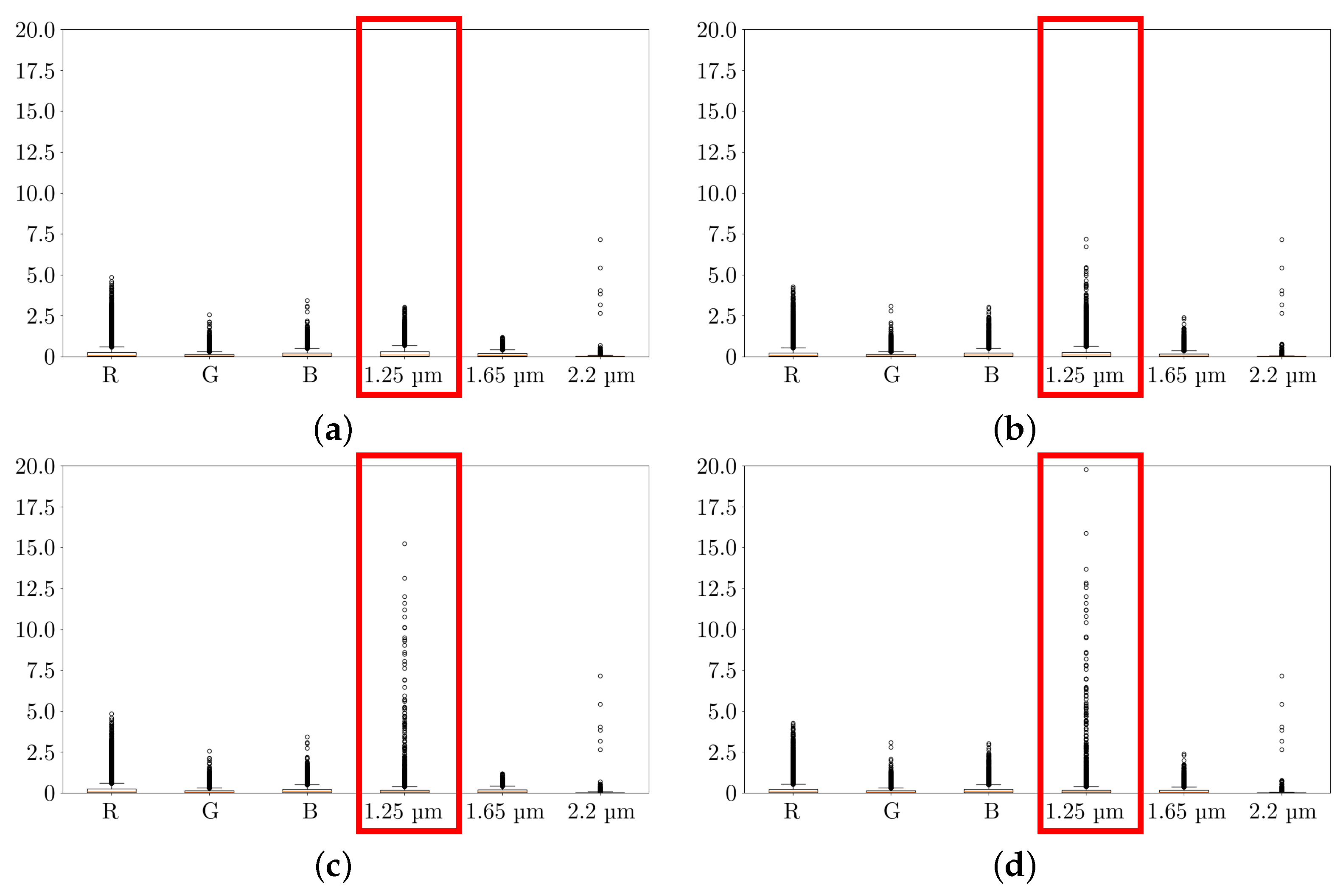
4.2.3. Local Analysis

The spatial distribution of the NG quality criterion (Section 2.4.1) was analysed for six selected spectral bands, which correspond to the two colour composites: RGB and the three selected SWIR bands (Section 3.1). To this end, box plots (Section 2.4.3) were generated. These series of six box plots are shown in Figure 9 (peri-urban dataset) and Figure 10 (urban case).
The contribution of the 1.35 μ m limit as compared with the 0.95 μ m one is highlighted in Figure 9, with the peri-urban dataset. The error associated with the 1.25 μ m spectral band is higher with CONDOR-2P than with Gain-2P, by choosing the 0.95 μ m limit, i.e., by applying (to this spectral band) the scale factor derived from the PAN image in the visible domain. However, if we choose the scale factor derived from the PAN image in the SWIR II domain, by moving the limit to 1.35 μ m , this error decreases (see box plots in red frames). In addition, this enhancement has no impact on the other analysed spectral bands, as their box plots remain strictly identical from one limit to another. Thus, by choosing the 1.35 μ m limit, Gain-2P and CONDOR-2P reduce the reconstruction errors according to all six displayed spectral bands.
The same cannot be concluded in the urban case. Contrary to previous analyses, box plots provide better results with the 0.95 μ m limit in terms of outliers. Indeed, the outliers in the 1.25 μ m spectral band increase when the limit changes from 0.95 μ m to 1.35 μ m , while those in the other spectral bands remained unchanged. Notably, the maximum normalised gap value of the distribution (not converted into percentage) increases from about 3 to 15.5 with Gain-2P and from about 7 to 20 with CONDOR-2P.
Hence, two opposite behaviours are highlighted:
  • In the peri-urban case, the error values from outliers in the SWIR domain were relatively low (i.e., close to the ones in the VNIR domain) with the first scale factor, and the second scale factor increased these error values with the 1.25 μ m spectral band. It is therefore preferable to set the limit to 1.35 μ m .
  • In the urban case, the error values from outliers in the SWIR spectral domain were much higher with the first scale factor, and the second one decreased them. The 0.95 μ m limit therefore provides better local results.
Nevertheless, pixels related to outliers represent a very small proportion of the scene. In particular, pixels such that NG > 2 (for at least one analysed spectral band) were restricted to 1 % of the scene. In addition, errors unrelated to outliers decrease with the 1.35 μ m limit, which thus reduces the average error. This can be visually seen in Figure 10. Thus, the local analysis of the urban dataset does not invalidate the better contribution of the 1.35 μ m limit. It only shows that this optimal choice still presents some limitations but that these limitations concern no more than 1 % of the urban scene.
To conclude, in Section 4.3 and Section 4.4, we systematically consider the 1.35 μ m limit to implement Gain-2P and CONDOR-2P.

4.3. Method Performance Assessment with One and Two PAN Channels

4.3.1. Global and Refined Analyses

Table 2 and Table 3 are exploited in this section, by focusing on the 1.35 μ m limit.
By comparing Gain with Gain-2P, one notices that results are similar in the VNIR spectral domain but better for Gain-2P in the SWIR spectral domain (about 50% of improvement for both datasets with the MNG criterion). This provides a 30% improvement in the whole reflective domain and for both datasets with the MNG criterion, as shown in Table 2 (see underlined values).
Similar comments can be made on CONDOR and CONDOR-2P. However, in this case, enhancements occur not only in the SWIR spectral domain but also in the VNIR spectral domain (60% and 24% improvement for both datasets with the MNG criterion, respectively). This is because the second PAN channel affects the spatial reorganisation step and improves the endmember assignment. This leads to an even more significant enhancement in the whole reflective domain: the MNG was reduced by about 45% for both datasets. This means a decrease by nearly a factor of two (see underlined values).
The most-important performance improvements between the methods using one and two PAN channels are thus related to the SWIR spectral domain (approximately 60% for both datasets). This is not an intermediate outcome as compared with performance in the reflective domain. Rather, this is a crucial result, because the second PAN channel was precisely introduced to enhance performance of the fusion methods in the SWIR spectral domain and particularly in complex urban environments.

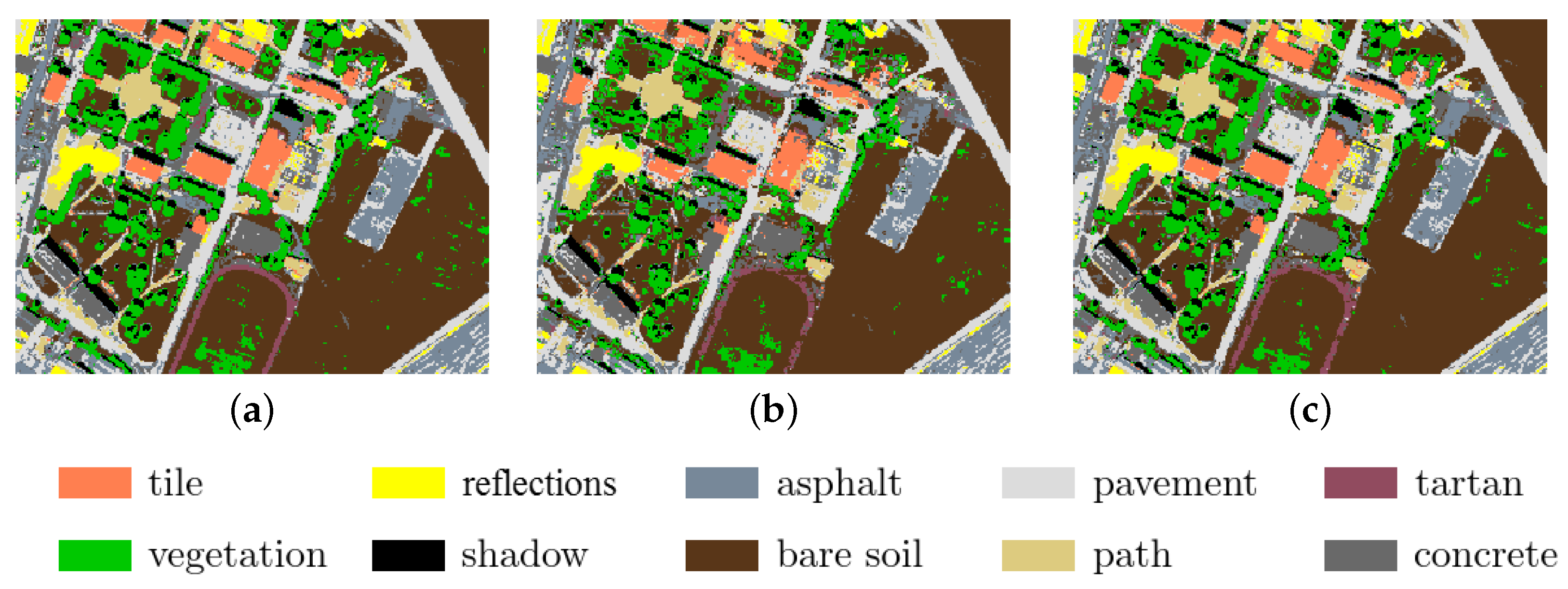
4.3.2. Land-Cover-Classification Maps

Classification maps (Section 2.4.4) were obtained for the REF and fused images. Three of them are shown in Figure 11 (peri-urban dataset) and Figure 12 (urban dataset): REF, CONDOR, and CONDOR-2P. Ten classes of materials were identified in the peri-urban scene, seven in the urban scene (see legends in Figure 11 and Figure 12). Among them, the “reflections” class corresponds to high spectral radiances caused by reflective materials like metal or glass (mainly cars and greenhouses). By following the training and validation process described in Section 2.4.4, we obtained a 92 % model accuracy in the urban case and 94 % in the peri-urban case.
Comparing the CONDOR and CONDOR-2P classification maps reveals a clear improvement in the spatial reorganisation with the latter method. Most reorganisation errors of CONDOR disappear with CONDOR-2P, in favour of a spatial structure closer to the original scene. The most-important enhancement concerns vegetation and is noticeable in both Figure 11 and Figure 12. Figure 11 also reveals that structure edges, as well as transitions between asphalt and bare soil, are better reconstructed by CONDOR-2P. The same observations can be made on the Gain and Gain-2P classification maps.
Table 4 (peri-urban) and Table 5 (urban) establish the overall accuracies derived from classification maps, for the specific pixel groups used for refined analyses. The corresponding masks are illustrated in Figure 13 for the peri-urban case.
The overall accuracy values highlight a significant gap between methods using one single PAN channel and methods using two PAN channels. In the peri-urban case (Table 4), CONDOR-2P gains 10% of overall accuracy as compared with CONDOR by considering the whole images and from 14% to 16% by focusing on spatially heterogeneous pixel groups (transition areas and a variance superior to 5). In addition, CONDOR-2P systematically obtains the highest overall accuracy values (as compared with all other methods): the latter are always higher than 92%, except for the spatially heterogeneous pixel groups, for which they still remain higher than 85%.
Similar comments can be made with the highest complexity dataset (Table 5), although the overall accuracy values are lower for all four methods. The gap between CONDOR-2P and CONDOR is also more important by considering the whole images and reaches 13%. However, the improvement still does not exceed 16% by focusing on spatially heterogeneous pixel groups. Comparing Gain and Gain-2P leads to the same observations, except that gaps are slightly reduced.
Nevertheless, there is an important difference in the urban case, which concerns shadowed pixels: this pixel group systematically provides the best overall accuracies (gap superior to 5% as compared with the other pixel groups). Yet, shadowed pixels are present in this dataset in a two-times higher proportion than in the peri-urban dataset. This confirms an important point documented in [44]: shadow pixels from urban scenes can be processed by the proposed methods.

4.4. Comparison of Gain-2P and CONDOR-2P

4.4.1. Global and Refined Analyses

Table 2 and Table 3 are exploited in this section, by choosing the 1.35 μ m limit.
The numerical results are systematically (i.e., whatever the dataset, the quality criterion, the spectral domain, or the selected pixel group) better with CONDOR-2P than with Gain-2P (see bold values). We noticed an error decrease from about 5% to 9% with CONDOR-2P in the peri-urban case for all three quality criteria, by considering the whole images and the reflective domain. This is an important result, which confirms the contribution of the mixed pixel preprocessing steps in the case of two PAN channels.
However, in the urban case, the gap between CONDOR-2P and Gain-2P was reduced. In the reflective domain, this gap did not exceed 4% with all three quality criteria regarding the whole images. These similar results were notably confirmed by identical SAM values. Nevertheless, despite close performance, CONDOR-2P still slightly outperformed Gain-2P, contrary to the case of one PAN channel for which Gain provides better results (see bold values). This outcome is important: it means that the combination of the two PAN channels contains enough information to provide enhancements with the preprocessing steps as compared with the fusion step only, contrary to one PAN channel.

4.4.2. Local Visual Analysis

Local visual results for the peri-urban and urban datasets are shown in Figure 14 and Figure 15, respectively.
Comparing the Gain-2P and CONDOR-2P fusion results obtained with the peri-urban dataset (Figure 14) reveals a higher-quality reconstruction for the latter method. Areas covered by single HS pixels, which are clearly distinguishable with Gain-2P, are correctly unmixed and reorganised in most parts of the scene with CONDOR-2P. This is particularly noticeable in the top and bottom thumbnails from Figure 14. In addition, spectral distortions (which have been pointed out in Section 4.2.1) are reduced with CONDOR-2P as compared with Gain-2P. This can be seen, for example, in the middle thumbnail from Figure 14.
However, with the urban dataset (Figure 15), the images fused by Gain-2P and CONDOR-2P are visually close. Except the top thumbnail where artefacts are reduced with CONDOR-2P (see white box), the only noticeable improvements in the SWIR spectral domain are related to reflective materials (see yellow boxes).

4.5. Synthesis

Several conclusions can be drawn from the different types of analysis performed in Section 4.1, Section 4.2, Section 4.3 AND Section 4.4. They concern results obtained by setting two important parameters. On the one hand, the (2.025–2.35 μ m) interval was selected to generate the second PAN channel in the SWIR II spectral domain (Section 4.1). However, the impact of the SWIR II interval on fusion quality was low, which reduces instrument constraints. On the other hand, the limit between the two Gain-2P application domains was set to 1.35 μ m (Section 4.2). In particular, the sensitivity study related to the limit choice systematically provides the best numerical results for CONDOR-2P and Gain-2P with the 1.35 μ m limit (as compared with the 0.95 μ m one), in the cases of both global and refined analyses.
Nevertheless, with the urban dataset, local analyses show that these numerical improvements are offset by an increase in the error values regarded as outliers (by using the NG criterion) in the spectral bands close to 1 μ m . However, note that these degradations mostly concern a reduced proportion of pixels (about 1%) and that the error from the rest of the image decreases with the 1.35 μ m limit (according to the NG criterion), leading to better global results with all quality criteria. Hence, we recommend to systematically set the limit to 1.35 μ m , regardless of the type of scene.
The most-important conclusion concerns the contribution of the new PAN channel on fusion quality (Section 4.3). Results obtained with the peri-urban and urban datasets reveal that taking into account a second PAN channel in the SWIR II spectral domain systematically enhances performance of fusion methods, both visually and numerically. Indeed, Gain-2P and CONDOR-2P obtain quality criteria values noticeably better than the ones of Gain and CONDOR for both datasets. This occurs not only in the SWIR spectral domain (up to a 60% decrease in the MNG values for both datasets) but also in the VNIR spectral domain in the CONDOR-2P case. Hence, numerical results were improved in the whole reflective domain (up to a 45% decrease in the MNG values for both datasets). The interest of this second PAN channel is thus demonstrated.
In addition, CONDOR-2P systematically outperformed all compared methods, including Gain-2P, both visually and numerically (Section 4.4). This is an enhancement as compared with one PAN channel, for which CONDOR cannot outperform Gain, due to a lack of significant information to find the optimal spatial reorganisations. This means the new PAN channel fixes the limitations of CONDOR and leads to quantified improvements. Therefore, the interest of the proposed preprocessing steps is justified with two PAN channels.
However, in practice, the contribution of CONDOR-2P can be mildly tempered. Numerically, CONDOR-2P provides slightly better numerical results than Gain-2P for nearly all quality criteria but without any important gap. Visually, its contribution is highlighted with the peri-urban dataset, where a large part of the scene (including the stadium and the roads) is better reconstructed. Yet, with the urban dataset, one distinguishes very few differences between the images fused by Gain-2P and CONDOR-2P. Therefore, the interest of CONDOR-2P preprocessing is clearly highlighted with peri-urban scenes and verified with urban scenes.

5. Discussion

Following the results shown in Section 4, some contributions and conclusions of our work can be pointed out.
Firstly, the importance of the proposed performance-assessment protocol has to be underlined. On the one hand, applying quality criteria to different spectral domains was essential to finding the current limitations of HS pansharpening methods in the SWIR domain and evaluating the improvements obtained with Gain-2P and CONDOR-2P. On the other hand, refined and local analyses are crucial to accurately evaluate the fusion quality according to the materials and the scene spatial complexity, in particular, for urban environments. Local analyses can induce different conclusions from global and refined analyses, as pointed out with the Gain-2P limit selection (Section 4.2.3). This complementarity has already been highlighted in previous work [44]. Yet, almost all HS pansharpening studies in the literature restrict their results to the whole images and HS spectral domains [8]. Refined analyses performed on selected pixel groups of interest are never proposed, and local analyses, in particular, land-cover-map generation (based on supervised classification and performed by machine learning), are only proposed in very few cases [47,48]. Therefore, we strongly encourage studies evaluating HS pansharpening methods on the reflective domain to use a robust and standardized performance-assessment protocol.
The most important point to stress is the contribution of the second PAN channel in the SWIR II spectral range. We clearly showed the gap between the fusion methods using one and two PAN channels, particularly in the SWIR spectral domain (as detailed in Section 4.3 and summarized in Section 4.5). This contribution is significant because, with one PAN channel covering the visible domain and HS images covering the reflective domain, spectral distortions can occur in fusion results, in particular beyond 1 μ m . This is especially the case for the methods of the CS fusion class. This main limitation of CS method was pointed out with various methods, including GS and GSA [22], as well as Gain, SOSU, and CONDOR in our previous works [44,45]. Therefore, using a second PAN channel in the SWIR spectral domain is an effective solution to overcome the most-important deficiency of CS methods.
Nevertheless, the question of instrumental feasibility has to be raised concerning the second PAN channel. In terms of storage, this could be achieved by using a satellite or airborne device with two carriers (for example, one for the HS camera and the other one for the two PAN cameras). In terms of instrument selection, only a few imaging systems integrate a PAN camera covering a broad spectral interval in the SWIR spectral domain [67]. Studies that propose adding a SWIR PAN channel to supplement an existing imaging system [68] are also rare. Indeed, marketed SWIR cameras are mostly HS instruments with low spatial resolution. In addition, they are often limited to spectral domains whose upper wavelength does not exceed 2 μ m , like the HySpex SWIR-640 camera [69]. There is no marketed broad-band SWIR camera for drone, airborne, or satellite imaging systems. Yet, this instrument concept must be taken into account to implement future imaging systems.
Meanwhile, a solution can be coupling various existing satellite or airborne instruments. As a starting point, one should favour instruments including both PAN and HS sensors in the visible and reflective domains, respectively, like PRISMA [17], HYPXIM [18,19], or EO-1 [20] (ALI + Hyperion). The second PAN channel could be obtained by using a SWIR II spectral band from an MS instrument, like Sentinel-2 [51]. The latter notably includes the (2.027–2.377 μ m) (S2A) and (2.001–2.371 μ m) (S2B) spectral bands, at a 20 m spatial resolution. This would, however, provide a large gap in terms of spatial resolution between the two PAN channels. In addition, one must ensure that the spatial resolution ratio between the Sentinel-2 SWIR II spectral band and the HS image is an integer, which is a strong constraint.

6. Conclusions

In this article, a second PAN channel was introduced in the SWIR II spectral domain to improve fusion-method performance. Two methods were adapted: Gain and CONDOR. The case of CONDOR was motivated by a dual interest: taking better account of the SWIR spectral bands and replacing the HS selection criterion by a new criterion that better exploits the spatial aspect of the scene in the optimisation problem of the reorganisation spatial step. Thus, the enhancements proposed to exploit the second PAN channel concern a new scale factor in the case of Gain-2P and an improvement in the cost function from the combinatory analysis in the case of CONDOR-2P.
After choosing an appropriate spectral interval to simulate the second PAN image and an optimal limit between Gain-2P application domains, the fusion methods adapted to one and two PAN channels were tested and compared for urban and peri-urban datasets. Visual and numerical (at global, refined, and local spatial scales) analyses, as well as supervised classification, pointed out the accuracy of the proposed performance-assessment protocol, by notably providing complementary results with the urban dataset. These analyses also highlighted two important contributions: first of all, the contribution of the second PAN channel, regardless of the method (confirmed, amongst others, by improvements in urban and peri-urbain environments reaching 45 % in the reflective domain and 60 % in the SWIR domain with the MNG criterion), and, more specifically, the contribution of CONDOR-2P (visually confirmed in peri-urban environment by a more accurate reconstruction than for Gain-2P).
The influence of this novel instrument concept on HS pansharpening still has to be evaluated in real conditions. In this study, we treated the reliability of Gain-2P and CONDOR-2P for environments of variable complexity (including vegetation, peri-urban structures, spaced houses, and a compact city centre). To supplement these analyses, future work will include evaluating the method performance with real (i.e., non-simulated) data in the case of one PAN channel (Gain and CONDOR). PRISMA [17] is a good fit, because it has already proved to be adapted to HS pansharpening with simulated data [70]. The next step will consist in performing an exhaustive sensitivity study of all four initial and extended methods, by evaluating the effects of the spatial resolution ratio (values from 2 to 10) and degradations caused by noise, Modulation Transfer Function (MTF), and deregistration. This latter degradation will be successively applied to each PAN channel and to the SWIR spectral bands of the HS image.
A last prospect would be extending the use of two PAN channels to other HS pansharpening methods. In this study, as we proposed the second PAN channel to reduce spectral distortions in the SWIR domain, we focused on CS methods that are the most sensitive ones to spectral distortions. Nevertheless, the interest of this novel instrument concept could also be demonstrated with more recent HS pansharpening classes, in particular, matrix factorization, Bayesian, and deep-learning methods.

Author Contributions

Conceptualization, Y.C., S.F., M.S., Y.D. and X.B.; data curation, Y.C.; formal analysis, Y.C., S.F. and X.B.; investigation, Y.C., S.F., Y.D. and X.B.; methodology, Y.C., S.F., M.S., Y.D. and X.B.; project administration, Y.C., S.F. and X.B.; software, Y.C.; supervision, S.F., M.S., V.C., Y.D. and X.B.; visualization, Y.C.; writing—original draft, Y.C.; writing—review and editing, Y.C., S.F., M.S., V.C., Y.D. and X.B. All authors have read and agreed to the published version of the manuscript.

Funding

This work has been done as part of a PhD co-funded by ONERA (the French aerospace lab) and Airbus Defence and Space. This research received no external funding.

Institutional Review Board Statement

Not applicable.

Informed Consent Statement

Not applicable.

Data Availability Statement

All exploited datasets have been extracted from airborne flight line hyperspectral images acquired with the HySpex Odin (FFI/NEO) instrument from the SYSIPHE imaging system (ONERA) [64] during the 2015 Canjuers airborne campaign [65]. They are not publicly available.

Acknowledgments

The authors want to thank Norsk Elektro Optikk AS (NEO) and the Norwegian Defence Research Establishment (FFI) who provided the HySpex Odin images. The authors are also grateful to Direction Générale de l’Armement (DGA) who funded the Canjuers airborne campaign.

Conflicts of Interest

The authors declare no conflict of interest.

Abbreviations

The following abbreviations are used at least twice in this manuscript and are not redefined:
CCCross Correlation (quality criterion)
CONDORCombinatorial Optimisation for 2D ORganisation (fusion method)
ERGASErreur Relative Globale Adimensionnelle de Synthèse (quality criterion)
GSGram-Schmidt (fusion method)
GSAGram–Schmidt adaptive (fusion method)
HSHyperSpectral (image)
MILPMixed Integer Linear Programming (optimisation problem)
MNGMean Normalised Gap (quality criterion)
MSMultiSpectral (image)
NGNormalised Gap (quality criterion)
NMSENormalised Mean Square Error (quality criterion)
NRMSENormalised Root Mean Square Error (quality criterion)
PANPANchromatic (image)
PRISMAPRecursore IperSpettrale della Missione Applicativa (instrument)
REFREFerence (image)
RGBRed-Green-Blue (colour composite)
RMSERoot Mean Square Error (quality criterion)
SAMSpectral Angle Mapper (quality criterion)
SLSTRSea and Land Surface Temperature Radiometer (instrument)
SOSUSpatially Organized Spectral Unmixing (fusion method)
SWIRShort-Wave InfraRed (1.0–2.5 μ m) spectral domain
VISVISible (0.4–0.8 μ m) spectral domain
VNIRVisible and Near-InfraRed (0.4–1.0 μ m) spectral domain

References

  1. Shalaby, A.; Tateishi, R. Remote sensing and GIS for mapping and monitoring land cover and land-use changes in the Northwestern coastal zone of Egypt. Appl. Geogr. 2007, 27, 28–41. [Google Scholar] [CrossRef]
  2. Miraglio, T.; Adeline, K.; Huesca, M.; Ustin, S.; Briottet, X. Monitoring LAI, chlorophylls, and carotenoids content of a woodland savanna using hyperspectral imagery and 3D radiative transfer modeling. Remote Sens. 2020, 12, 28. [Google Scholar] [CrossRef] [Green Version]
  3. Hu, S.; Wang, L. Automated urban land-use classification with remote sensing. Int. J. Remote Sens. 2013, 34, 790–803. [Google Scholar] [CrossRef]
  4. Donnay, J.P.; Barnsley, M.J.; Longley, P.A. Remote Sensing and Urban Analysis; CRC Press: Boca Raton, FL, USA, 2000. [Google Scholar]
  5. Sabins, F.F. Remote Sensing: Principles and Applications; Waveland Press: Long Grove, IN, USA, 2007. [Google Scholar]
  6. Benediktsson, J.A.; Ghamisi, P. Spectral-Spatial Classification of Hyperspectral Remote Sensing Images; Artech House: Norwood, MA, USA, 2015. [Google Scholar]
  7. Lier, P.; Valorge, C.; Briottet, X. Satellite Imagery from Acquisition Principle to Processing of Optical Images for Observing the Earth; CEPADUES Editions: Toulouse, France, 2012. [Google Scholar]
  8. Loncan, L.; De Almeida, L.B.; Bioucas-Dias, J.M.; Briottet, X.; Chanussot, J.; Dobigeon, N.; Fabre, S.; Liao, W.; Licciardi, G.A.; Simoes, M.; et al. Hyperspectral pansharpening: A review. IEEE Geosci. Remote Sens. Mag. 2015, 3, 27–46. [Google Scholar] [CrossRef] [Green Version]
  9. Zhang, Y. Understanding image fusion. Photogramm. Eng. Remote Sens. 2004, 70, 657–661. [Google Scholar]
  10. Gleyzes, M.A.; Perret, L.; Kubik, P. Pleiades system architecture and main performances. Int. Arch. Photogramm. Remote Sens. Spat. Inf. Sci. 2012, 39, 537–542. [Google Scholar] [CrossRef] [Green Version]
  11. Bicknell, W.E.; Digenis, C.J.; Forman, S.E.; Lencioni, D.E. EO-1 advanced land imager. In Earth Observing Systems IV; International Society for Optics and Photonics: Bellingham, MA, USA, 1999; Volume 3750, pp. 80–88. [Google Scholar]
  12. Porter, W.M.; Enmark, H.T. A system overview of the airborne visible/infrared imaging spectrometer (AVIRIS). In Imaging Spectroscopy I; International Society for Optics and Photonics: Bellingham, MA, USA, 1987; Volume 834, pp. 22–31. [Google Scholar]
  13. Cocks, T.; Jenssen, R.; Stewart, A.; Wilson, I.; Shields, T. The HyMap airborne hyperspectral sensor: The system, calibration and performance. In Proceedings of the 1st EARSeL workshop on Imaging Spectroscopy, Zurich, Switzerland, 6–8 October 1998; pp. 37–42. [Google Scholar]
  14. Briottet, X.; Feret, J.B.; Jacquemoud, S.; Lelong, C.; Rocchini, D.; Schaepman, M.E.; Sheeren, D.; Skidmore, A.; Somers, B.; Gomez, C.; et al. European Hyperspectral Explorer: HYPEX-2—A new space mission for vegetation biodiversity, bare continental surfaces, coastal zones and urban area ecosystems. In Proceedings of the 10th EARSeL SIG Imaging Spectroscopy Workshop, Zurich, Switzerland, 19–21 April 2017. [Google Scholar]
  15. Stuffler, T.; Kaufmann, C.; Hofer, S.; Förster, K.; Schreier, G.; Mueller, A.; Eckardt, A.; Bach, H.; Penné, B.; Benz, U.; et al. The EnMAP hyperspectral imager—An advanced optical payload for future applications in Earth observation programmes. Acta Astronaut. 2007, 61, 115–120. [Google Scholar] [CrossRef]
  16. Pearlman, J.; Carman, S.; Segal, C.; Jarecke, P.; Clancy, P.; Browne, W. Overview of the Hyperion imaging spectrometer for the NASA EO-1 mission. IGARSS 2001. Scanning the Present and Resolving the Future. In Proceedings of the IEEE 2001 International Geoscience and Remote Sensing Symposium (Cat. No. 01CH37217), Sydney, NSW, Australia, 9–13 July 2001; IEEE: Piscataway, NJ, USA, 2001; Volume 7, pp. 3036–3038. [Google Scholar]
  17. Galeazzi, C.; Sacchetti, A.; Cisbani, A.; Babini, G. The PRISMA program. In Proceedings of the IGARSS 2008—2008 IEEE International Geoscience and Remote Sensing Symposium, Boston, MA, USA, 8–11 July 2008; IEEE: Piscataway, NJ, USA, 2008; Volume 4, pp. IV-105–IV-108. [Google Scholar]
  18. Michel, S.; Gamet, P.; Lefevre-Fonollosa, M.J. HYPXIM—A hyperspectral satellite defined for science, security and defence users. In Proceedings of the 2011 3rd Workshop on Hyperspectral Image and Signal Processing: Evolution in Remote Sensing (WHISPERS), Lisbon, Portugal, 6–9 June 2011; IEEE: Piscataway, NJ, USA, 2011; pp. 1–4. [Google Scholar]
  19. Briottet, X.; Marion, R.; Carrere, V.; Jacquemoud, S.; Chevrel, S.; Prastault, P.; D’oria, M.; Gilouppe, P.; Hosford, S.; Lubac, B.; et al. HYPXIM: A new hyperspectral sensor combining science/defence applications. In Proceedings of the 2011 3rd Workshop on Hyperspectral Image and Signal Processing: Evolution in Remote Sensing (WHISPERS), Lisbon, Portugal, 6–9 June 2011; IEEE: Piscataway, NJ, USA, 2011; pp. 1–4. [Google Scholar]
  20. Ungar, S.G.; Pearlman, J.S.; Mendenhall, J.A.; Reuter, D. Overview of the earth observing one (EO-1) mission. IEEE Trans. Geosci. Remote Sens. 2003, 41, 1149–1159. [Google Scholar] [CrossRef]
  21. Cetin, M.; Musaoglu, N. Merging hyperspectral and panchromatic image data: Qualitative and quantitative analysis. Int. J. Remote Sens. 2009, 30, 1779–1804. [Google Scholar] [CrossRef]
  22. Aiazzi, B.; Baronti, S.; Selva, M. Improving component substitution pansharpening through multivariate regression of MS + Pan data. IEEE Trans. Geosci. Remote Sens. 2007, 45, 3230–3239. [Google Scholar] [CrossRef]
  23. Saroglu, E.; Bektas, F.; Musaoglu, N.; Goksel, C. Fusion of multisensor remote sensing data: Assessing the quality of resulting images. Int. Arch. Photogram. Remote Sens. Spatial. Inform. Sci. 2004, 35, 575–579. [Google Scholar]
  24. Vivone, G.; Alparone, L.; Chanussot, J.; Dalla Mura, M.; Garzelli, A.; Licciardi, G.A.; Restaino, R.; Wald, L. A critical comparison among pansharpening algorithms. IEEE Trans. Geosci. Remote Sens. 2014, 53, 2565–2586. [Google Scholar] [CrossRef]
  25. Loncan, L. Fusion of Hyperspectral and Panchromatic Images with very High Spatial Resolution. Ph.D. Thesis, Université Grenoble Alpes, Grenoble, France, 2016. [Google Scholar]
  26. Aiazzi, B.; Alparone, L.; Baronti, S.; Garzelli, A.; Selva, M. MTF-tailored multiscale fusion of high-resolution MS and Pan imagery. Photogramm. Eng. Remote Sens. 2006, 72, 591–596. [Google Scholar] [CrossRef]
  27. Vivone, G.; Restaino, R.; Dalla Mura, M.; Licciardi, G.; Chanussot, J. Contrast and error-based fusion schemes for multispectral image pansharpening. IEEE Geosci. Remote Sens. Lett. 2013, 11, 930–934. [Google Scholar] [CrossRef] [Green Version]
  28. Dong, W.; Xiao, S.; Xue, X.; Qu, J. An improved hyperspectral pansharpening algorithm based on optimized injection model. IEEE Access 2019, 7, 16718–16729. [Google Scholar] [CrossRef]
  29. Qu, J.; Li, Y.; Dong, W. A new hyperspectral pansharpening method based on guided fliter. In Proceedings of the 2017 IEEE International Geoscience and Remote Sensing Symposium (IGARSS), Fort Worth, TX, USA, 23–28 July 2017; IEEE: Piscataway, NJ, USA, 2017; pp. 5125–5128. [Google Scholar]
  30. Qu, J.; Li, Y.; Dong, W. Hyperspectral pansharpening with guided filter. IEEE Geosci. Remote Sens. Lett. 2017, 14, 2152–2156. [Google Scholar] [CrossRef]
  31. Qu, J.; Li, Y.; Dong, W. Fusion of hyperspectral and panchromatic images using an average filter and a guided filter. J. Vis. Commun. Image Represent. 2018, 52, 151–158. [Google Scholar] [CrossRef]
  32. Dong, W.; Xiao, S. An Adaptive Weighted Regression and Guided Filter Hybrid Method for Hyperspectral Pansharpening. TIIS 2019, 13, 327–346. [Google Scholar]
  33. Elad, M.; Aharon, M. Image denoising via sparse and redundant representations over learned dictionaries. IEEE Trans. Image Process. 2006, 15, 3736–3745. [Google Scholar] [CrossRef]
  34. Wei, Q.; Bioucas-Dias, J.; Dobigeon, N.; Tourneret, J.Y. Hyperspectral and multispectral image fusion based on a sparse representation. IEEE Trans. Geosci. Remote Sens. 2015, 53, 3658–3668. [Google Scholar] [CrossRef] [Green Version]
  35. Lin, H.; Zhang, A. Fusion of hyperspectral and panchromatic images using improved HySure method. In Proceedings of the 2017 2nd International Conference on Image, Vision and Computing (ICIVC), Chengdu, China, 2–4 June 2017; IEEE: Piscataway, NJ, USA, 2017; pp. 489–493. [Google Scholar]
  36. Huang, Z.; Chen, Q.; Shen, Y.; Chen, Q.; Liu, X. An improved variational method for hyperspectral image pansharpening with the constraint of Spectral Difference Minimization. Int. Arch. Photogramm. Remote Sens. Spat. Inf. Sci. 2017, 42, 753–760. [Google Scholar] [CrossRef] [Green Version]
  37. Yokoya, N.; Yairi, T.; Iwasaki, A. Coupled nonnegative matrix factorization unmixing for hyperspectral and multispectral data fusion. IEEE Trans. Geosci. Remote Sens. 2011, 50, 528–537. [Google Scholar] [CrossRef]
  38. Karoui, M.S.; Deville, Y.; Benhalouche, F.Z.; Boukerch, I. Hypersharpening by joint-criterion nonnegative matrix factorization. IEEE Trans. Geosci. Remote Sens. 2016, 55, 1660–1670. [Google Scholar] [CrossRef]
  39. Kaur, G.; Saini, K.S.; Singh, D.; Kaur, M. A Comprehensive Study on Computational Pansharpening Techniques for Remote Sensing Images. In Archives of Computational Methods in Engineering; Springer: Berlin/Heidelberg, Germany, 2021; pp. 1–18. [Google Scholar]
  40. Li, K.; Xie, W.; Du, Q.; Li, Y. DDLPS: Detail-based deep Laplacian pansharpening for hyperspectral imagery. IEEE Trans. Geosci. Remote Sens. 2019, 57, 8011–8025. [Google Scholar] [CrossRef]
  41. Xie, W.; Lei, J.; Cui, Y.; Li, Y.; Du, Q. Hyperspectral pansharpening with deep priors. IEEE Trans. Neural Netw. Learn. Syst. 2019, 31, 1529–1543. [Google Scholar] [CrossRef]
  42. Xie, W.; Cui, Y.; Li, Y.; Lei, J.; Du, Q.; Li, J. HPGAN: Hyperspectral Pansharpening Using 3-D Generative Adversarial Networks. IEEE Trans. Geosci. Remote Sens. 2021, 59, 463–477. [Google Scholar] [CrossRef]
  43. Sun, L.; Wu, F.; He, C.; Zhan, T.; Liu, W.; Zhang, D. Weighted Collaborative Sparse and L1/2 Low-Rank Regularizations with Superpixel Segmentation for Hyperspectral Unmixing. IEEE Geosci. Remote Sens. Lett. 2020, 1–5. [Google Scholar] [CrossRef]
  44. Constans, Y.; Fabre, S.; Seymour, M.; Crombez, V.; Briottet, X.; Deville, Y. Fusion of hyperspectral and panchromatic data by spectral unmixing in the reflective domain. ISPRS-Int. Arch. Photogramm. Remote Sens. Spat. Inf. Sci. 2020, XLIII-B3-2020, 567–574. [Google Scholar] [CrossRef]
  45. Constans, Y.; Fabre, S.; Carfantan, H.; Seymour, M.; Crombez, V.; Briottet, X.; Deville, Y. Fusion of panchromatic and hyperspectral images in the reflective domain by a combinatorial approach and application to urban landscape. In Proceedings of the 2021 IEEE International Geoscience and Remote Sensing Symposium IGARSS, Brussels, Belgium, 11–16 July 2021; IEEE: Piscataway, NJ, USA, 2021; pp. 2648–2651. [Google Scholar]
  46. Lu, D.; Hetrick, S.; Moran, E. Land cover classification in a complex urban-rural landscape with QuickBird imagery. Photogramm. Eng. Remote Sens. 2010, 76, 1159–1168. [Google Scholar] [CrossRef] [Green Version]
  47. Liao, W.; Huang, X.; Van Coillie, F.; Gautama, S.; Pižurica, A.; Philips, W.; Liu, H.; Zhu, T.; Shimoni, M.; Moser, G.; et al. Processing of multiresolution thermal hyperspectral and digital color data: Outcome of the 2014 IEEE GRSS data fusion contest. IEEE J. Sel. Top. Appl. Earth Obs. Remote Sens. 2015, 8, 2984–2996. [Google Scholar] [CrossRef]
  48. Liao, W.; Huang, X.; Van Coillie, F.; Thoonen, G.; Pižurica, A.; Scheunders, P.; Philips, W. Two-stage fusion of thermal hyperspectral and visible RGB image by PCA and Guided filter. In Proceedings of the 2015 7th Workshop on Hyperspectral Image and Signal Processing: Evolution in Remote Sensing (WHISPERS), Tokyo, Japan, 2–5 June 2015; IEEE: Piscataway, NJ, USA, 2015; pp. 1–4. [Google Scholar]
  49. Forrest, J.J.H. COIN Branch and Cut. COIN-OR. Available online: http://www.coin-or.org (accessed on 5 November 2021).
  50. Makhorin, A. GLPK (GNU Linear Programming Kit). 2008. Available online: http://www.gnu.org/s/glpk/glpk.html (accessed on 5 November 2021).
  51. Drusch, M.; Del Bello, U.; Carlier, S.; Colin, O.; Fernandez, V.; Gascon, F.; Hoersch, B.; Isola, C.; Laberinti, P.; Martimort, P.; et al. Sentinel-2: ESA’s optical high-resolution mission for GMES operational services. Remote Sens. Environ. 2012, 120, 25–36. [Google Scholar] [CrossRef]
  52. Donlon, C.; Berruti, B.; Buongiorno, A.; Ferreira, M.H.; Féménias, P.; Frerick, J.; Goryl, P.; Klein, U.; Laur, H.; Mavrocordatos, C.; et al. The global monitoring for environment and security (GMES) sentinel-3 mission. Remote Sens. Environ. 2012, 120, 37–57. [Google Scholar] [CrossRef]
  53. Wald, L.; Ranchin, T.; Mangolini, M. Fusion of satellite images of different spatial resolutions: Assessing the quality of resulting images. Photogramm. Eng. Remote Sens. 1997, 63, 691–699. [Google Scholar]
  54. Pei, W.; Wang, G.; Yu, X. Performance evaluation of different references based image fusion quality metrics for quality assessment of remote sensing Image fusion. In Proceedings of the 2012 IEEE International Geoscience and Remote Sensing Symposium, Munich, Germany, 22–27 July 2012; IEEE: Piscataway, NJ, USA, 2012; pp. 2280–2283. [Google Scholar]
  55. Canny, J. A computational approach to edge detection. IEEE Trans. Pattern Anal. Mach. Intell. 1986, 6, 679–698. [Google Scholar] [CrossRef]
  56. Nagao, M.; Matsuyama, T.; Ikeda, Y. Region extraction and shape analysis in aerial photographs. Comput. Graph. Image Process. 1979, 10, 195–223. [Google Scholar] [CrossRef]
  57. Hayslett, H.T. Statistics; Elsevier: Amsterdam, The Netherlands, 2014. [Google Scholar]
  58. Williamson, D.F.; Parker, R.A.; Kendrick, J.S. The box plot: A simple visual method to interpret data. Ann. Intern. Med. 1989, 110, 916–921. [Google Scholar] [CrossRef]
  59. Chutia, D.; Bhattacharyya, D.; Sarma, K.K.; Kalita, R.; Sudhakar, S. Hyperspectral remote sensing classifications: A perspective survey. Trans. GIS 2016, 20, 463–490. [Google Scholar] [CrossRef]
  60. Belgiu, M.; Drăguţ, L. Random forest in remote sensing: A review of applications and future directions. ISPRS J. Photogramm. Remote Sens. 2016, 114, 24–31. [Google Scholar] [CrossRef]
  61. Browne, M.W. Cross-validation methods. J. Math. Psychol. 2000, 44, 108–132. [Google Scholar] [CrossRef] [Green Version]
  62. Purushotham, S.; Tripathy, B. Evaluation of classifier models using stratified tenfold cross validation techniques. In International Conference on Computing and Communication Systems; Springer: Berlin/Heidelberg, Germany, 2011; pp. 680–690. [Google Scholar]
  63. Stehman, S.V. Selecting and interpreting measures of thematic classification accuracy. Remote Sens. Environ. 1997, 62, 77–89. [Google Scholar] [CrossRef]
  64. Rousset-Rouviere, L.; Coudrain, C.; Fabre, S.; Baarstad, I.; Fridman, A.; Løke, T.; Blaaberg, S.; Skauli, T. Sysiphe, an airborne hyperspectral imaging system for the VNIR-SWIR-MWIR-LWIR region. In Proceedings of the 7th EARSeL Workshop on Imaging Spectroscopy, Edinburgh, UK, 11–13 April 2011; pp. 1–12. [Google Scholar]
  65. Rousset-Rouviere, L.; Coudrain, C.; Fabre, S.; Ferrec, Y.; Poutier, L.; Viallefont, F.; Rivière, T.; Ceamanos, X.; Loke, T.; Fridman, A.; et al. SYSIPHE, an airborne hyperspectral imaging system from visible to thermal infrared. Results from the 2015 airborne campaign. In Proceedings of the 10th EARSEL SIG Imaging Spectroscopy, Zurich, Switzerland, 19–21 April 2017. [Google Scholar]
  66. Comaniciu, D.; Meer, P. Mean shift: A robust approach toward feature space analysis. IEEE Trans. Pattern Anal. Mach. Intell. 2002, 24, 603–619. [Google Scholar] [CrossRef] [Green Version]
  67. Madani, A.A. Selection of the optimum Landsat Thematic Mapper bands for automatic lineaments extraction, Wadi Natash area, south eastern desert, Egypt. Asian J. Geoinform. 2001, 3, 71–76. [Google Scholar]
  68. Yuan, Y.; Zhang, L.; Su, L.; Ye, Z. Study on shortwave infrared multispectral horizontal imgaing performance under haze weather condition. In AOPC 2019: Optical Spectroscopy and Imaging; International Society for Optics and Photonics: Bellingham, MA, USA, 2019; Volume 11337, p. 113370M. [Google Scholar]
  69. HySpex SWIR-640. Available online: https://www.hyspex.com/hyspex-products/hyspex-classic/hyspex-swir-640/ (accessed on 27 September 2021).
  70. Aiazzi, B.; Alparone, L.; Baronti, S.; Garzelli, A.; Selva, M. Pansharpening of hyperspectral images: A critical analysis of requirements and assessment on simulated PRISMA data. In Image and Signal Processing for Remote Sensing XIX; International Society for Optics and Photonics: Bellingham, MA, USA, 2013; Volume 8892, p. 889203. [Google Scholar]
Figure 1. Gain-2P method principle.
Remotesensing 14 00113 g001
Figure 2. Flow chart of the CONDOR method [44]. The preprocessing steps are framed in green, with the fusion step in blue; the improved CONDOR-2P steps are identified in red.
Remotesensing 14 00113 g002
Figure 3. Principle of the spatial-reorganisation step performed by a combinatorial analysis.
Remotesensing 14 00113 g003
Figure 4. Spectrum of a pixel extracted from the reference (REF) image from the “Toulon” dataset (Section 3.2): identification of the tested spectral intervals in the SWIR II domain (broad band in brown, Sentinel-2 in green, and Sentinel-3 in orange), and three possible limits separating the Gain-2P application domains (in red). The represented spectral bands are the ones whose atmospheric transmission is superior to 80 % .
Remotesensing 14 00113 g004
Figure 5. “Stadium” dataset (spatial resolutions in brackets; RGB representation for HS images). (a) REF (1.5 m), (b) HS (6 m), (c) PAN, visible (1.5 m), and (d) PAN, SWIR (1.5 m).
Remotesensing 14 00113 g005
Figure 6. “Toulon” dataset (spatial resolutions in brackets; RGB representation for HS images). (a) REF (1.5 m), (b) HS (6 m), (c) PAN, visible (1.5 m), (d) PAN, SWIR (1.5 m).
Remotesensing 14 00113 g006
Figure 7. “Gardanne” dataset (spatial resolutions in brackets; RGB representation for HS images). (a) REF (1.5 m), (b) HS (6 m), (c) PAN, visible (1.5 m), and (d) PAN, SWIR (1.5 m).
Remotesensing 14 00113 g007
Figure 8. “Toulon” peri-urban dataset: global visual results (SWIR colour composite images; spatial resolution: 1.5 m; Gain-2P limit in brackets). (a) REF, (b) PAN visible, (c) PAN SWIR II, (d) Gain, (e) Gain-2P ( 0.95 μ m ), (f) Gain-2P ( 1.35 μ m ), (g) CONDOR, (h) CONDOR-2P ( 0.95 μ m ), and (i) CONDOR-2P ( 1.35 μ m ).
Remotesensing 14 00113 g008
Figure 9. “Toulon” peri-urban dataset: box plots and outliers depicting the distribution of the NG criterion (not converted into percentage), for the six analysed spectral bands. (a) Gain-2P ( 0.95 μ m ), (b) CONDOR-2P ( 0.95 μ m ), (c) Gain-2P ( 1.35 μ m ), and (d) CONDOR-2P ( 1.35 μ m ).
Remotesensing 14 00113 g009
Figure 10. “Gardanne” urban dataset: box plots and outliers depicting the distribution of the NG criterion (not converted into percentage), for the six analysed spectral bands. (a) Gain-2P— 0.95 μ m , (b) CONDOR-2P— 0.95 μ m , (c) Gain-2P— 1.35 μ m , and (d) CONDOR-2P— 1.35 μ m .
Remotesensing 14 00113 g010
Figure 11. “Toulon” peri-urban dataset: land-cover-classification maps of fused and REF images. (a) REF, (b) CONDOR, and (c) CONDOR-2P.
Remotesensing 14 00113 g011
Figure 12. “Gardanne” urban dataset: land-cover-classification maps of REF and fused images. The “reflections” class corresponds to high spectral radiances caused by reflective materials like metal (e.g., cars) or glass (e.g., greenhouses). (a) REF, (b) CONDOR, and (c) CONDOR-2P.
Remotesensing 14 00113 g012
Figure 13. “Toulon” peri-urban dataset: masks corresponding to the located specific pixel groups (pixels belonging to the masks identified in magenta; associated pixel proportions in percent). (a) Transitions areas: 50%, (b) shadowed pixels: 4%, (c) HS pixels with variance < 5: 64%, (d) HS pixels with variance [ 5 ; 10 ] : 14%, (e) HS pixels with variance [ 10 ; 15 ] : 7%, and (f) HS pixels with variance > 15: 16%.
Remotesensing 14 00113 g013
Figure 14. “Toulon” peri-urban dataset: local visual results (SWIR colour composite images; spatial resolution: 1.5 m).
Remotesensing 14 00113 g014
Figure 15. “Gardanne” urban dataset: local visual results (SWIR colour composite images; spatial resolution: 1.5 m).
Remotesensing 14 00113 g015
Table 1. “Stadium”: quality criteria calculated on the whole images, for the three proposed SWIR II PAN spectral bands. The optimal values (according to the SWIR II PAN domain only) are identified in bold.
SWIR II PAN
Domain (μm)
MethodSpectral DomainMNG (%)SAM ( )RMSEERGASCC
(2.0–2.5) Gain-2PVNIR4.22.54.92.00.96
SWIR3.20.91.91.30.96
Reflective3.72.63.81.70.96
CONDOR-2PVNIR3.72.24.71.90.96
SWIR3.00.92.01.30.96
Reflective3.42.33.71.60.96
(2.025–2.35) Gain-2PVNIR4.22.54.92.00.96
SWIR3.20.91.91.30.96
Reflective3.72.63.81.70.96
CONDOR-2PVNIR3.72.24.71.90.96
SWIR3.00.91.91.30.96
Reflective3.32.33.61.60.96
(2.2–2.3) Gain-2PVNIR4.22.54.92.00.96
SWIR3.10.91.91.30.96
Reflective3.72.63.81.70.96
CONDOR-2PVNIR3.72.24.71.90.96
SWIR2.90.91.91.30.96
Reflective3.32.33.71.60.96
Table 2. “Toulon” and “Gardanne” datasets: quality criteria calculated on the whole images. The optimal values in the reflective domain are in bold (by comparing the methods) and underlined (by comparing the PAN configurations).
PAN ChannelsMethodSpectral
Domain
“Toulon”“Gardanne”
MNG
(%)
SAM (°)RMSEMNG
(%)
SAM (°)RMSE
1 PAN channel GainVNIR6.83.77.213.26.29.1
SWIR11.11.73.619.62.85.3
Reflective9.03.85.716.46.57.5
CONDORVNIR8.64.58.617.07.811.7
SWIR13.92.24.024.13.56.3
Reflective11.24.76.720.58.19.4
2 PAN channels,
0.95 μ m limit
Gain-2PVNIR6.93.77.313.36.39.2
SWIR7.51.76.012.82.88.6
Reflective7.24.46.613.07.48.9
CONDOR-2PVNIR6.53.56.713.06.28.7
SWIR7.01.65.212.22.67.6
Reflective6.84.16.012.57.18.1
2 PAN channels,
1.35 μ m limit
Gain-2PVNIR6.83.77.213.26.29.1
SWIR5.81.83.49.73.14.6
Reflective6.33.85.711.56.47.2
CONDOR-2PVNIR6.53.56.612.96.18.6
SWIR5.51.73.29.62.94.6
Reflective6.03.65.211.36.46.9
Table 3. “Toulon” and “Gardanne” datasets: quality criteria calculated on transition areas. The optimal values are in bold (by comparing the methods) and underlined (by comparing the PAN configurations).
PAN ChannelsMethodSpectral
Domain
“Toulon”“Gardanne”
MNG
(%)
SAM (°)RMSEMNG
(%)
SAM (°)RMSE
1 PAN channel GainVNIR10.15.49.716.47.810.7
SWIR16.72.44.723.13.46.4
Reflective13.45.77.719.78.08.8
CONDORVNIR11.96.311.019.99.313.0
SWIR20.13.05.127.44.17.3
Reflective16.06.58.623.79.510.6
2 PAN channels,
0.95 μ m limit
Gain-2PVNIR10.25.49.816.57.810.8
SWIR11.02.47.815.53.410.0
Reflective10.56.48.816.09.010.3
CONDOR-2PVNIR9.65.18.915.97.610.0
SWIR10.32.26.814.83.28.7
Reflective9.96.07.915.38.69.4
2 PAN channels,
1.35 μm limit
Gain-2PVNIR10.15.49.716.47.810.7
SWIR8.82.84.611.83.65.4
Reflective9.45.67.614.18.08.5
CONDOR-2PVNIR9.65.18.815.87.510.0
SWIR8.22.54.311.53.45.4
Reflective8.95.37.013.77.88.0
Table 4. “Toulon” peri-urban dataset: overall accuracy values (in %) for different pixel groups (depicted in Figure 13).
Pixel GroupProportionGainCONDORGain-2PCONDOR-2P
Whole images100%85829192
Sunlit pixels96%85829192
Shadowed pixels4%89879192
HS pixels with variance < 564%91889595
HS pixels with variance [ 5 ; 10 ] 14%77738789
HS pixels with variance [ 10 ; 15 ] 7%72718485
HS pixels with variance > 1516%74718485
Pixels in transition areas50%76738687
Pixels out of transition areas50%94919797
Table 5. “Gardanne” urban dataset: overall accuracy values (in %) for different pixel groups.
Pixel GroupProportionGainCONDORGain-2PCONDOR-2P
Whole images100%78738786
Sunlit pixels92%77718686
Shadowed pixels8%94949595
HS pixels with variance < 530%84779090
HS pixels with variance [ 5 ; 10 ] 23%78728787
HS pixels with variance [ 10 ; 15 ] 15%76708686
HS pixels with variance > 1532%74718383
Pixels in transition areas62%74708484
Pixels out of transition areas38%85779190
Publisher’s Note: MDPI stays neutral with regard to jurisdictional claims in published maps and institutional affiliations.

