Machine Learning in Evaluating Multispectral Active Canopy Sensor for Prediction of Corn Leaf Nitrogen Concentration and Yield

Abstract

Applying the optimum rate of fertilizer nitrogen (N) is a critical factor for field management. Multispectral information collected by active canopy sensors can potentially indicate the leaf N status and aid in predicting grain yield. Crop Circle multispectral data were acquired with the purpose of measuring the reflectance data to calculate vegetation indices (VIs) at different growth stages. Applying the optimum rate of fertilizer N can have a considerable impact on grain yield and profitability. The objectives of this study were to evaluate the reliability of a handheld Crop Circle ACS-430, to estimate corn leaf N concentration and predict grain yield of corn using machine learning (ML) models. The analysis was conducted using four ML models to identify the best prediction model for measurements acquired with a Crop Circle ACS-430 field sensor at three growth stages. Four fertilizer N levels from deficient to excessive in 50/50 spilt were applied to corn at 1–2 leaves, with visible leaf collars (V1–V2 stage) and at the V6–V7 stage to establish widely varying N nutritional status. Crop Circle spectral observations were used to derive 25 VIs for different growth stages (V4, V6, and VT) of corn at the W. B. Andrews Agricultural Systems farm of Mississippi State University. Multispectral raw data, along with Vis, were used to quantify leaf N status and predict the yield of corn. In addition, the accuracy of wavelength-based and VI-based models were compared to examine the best model inputs. Due to limited observed data, the stratification approach was used to split data to train and test set to obtain balanced data for each stage. Repeated cross validation (RCV) was then used to train the models. Results showed that the Simplified Canopy Chlorophyll Content Index (SCCCI) and Red-edge ratio vegetation index (RERVI) were the most effective VIs for estimating leaf N% and that SCCCI, Red-edge chlorophyll index (CIRE), RERVI, Soil Adjusted Vegetation Index (SAVI), and Normalized Difference Vegetation Index (NDVI) were the most effective VIs for predicting corn grain yield. Additionally, among the four ML models utilized in this research, support vector regression (SVR) achieved the most accurate results for estimating leaf N concentration using either spectral bands or VIs as the model inputs.

1. Introduction

Agricultural products play a major role in feeding the world’s population and have a remarkable impact on people’s life and work by providing food, feed, and fuels. It is estimated that land used for agricultural purposes expanded by around 10 million ha/y from 1980 to 2007 [1] to meet the needs of a growing population, changing diets, and emerging demand for biofuels. However, from 2010–2012, around 870 million people across the globe did not meet their minimum dietary energy needs due to insufficient foodstuffs [2]. The United States Department of Agriculture (USDA) reported that, in 2019, approximately 36 million ha of corn was planted in the US and 0.27 million ha in Mississippi and 11.3 ton/ha and 11.7 ton/ha of corn grain was harvested in the US and Mississippi, respectively [3]. The importance of increasing production efficiency to meet global food demands is critical to maintaining or increasing economic viability while minimizing environmental hazards.

Nitrogen (N) is a primary nutrient required for plant growth, development, and the reproduction of healthy plants, and it plays a key role in the developing phenological stages of corn, since N is directly related to photosynthesis [4]. An increase in fertilizer N application rates has contributed substantially to an increase in the yield of grain crops throughout the world [5]. However, applying fertilizer N in excess of crop demand can result in decreased economic returns, low Nitrogen Use Efficiency (NUE), poor nutritional quality, and a negative environmental impact [6,7]. A deficiency of N causes plants to senesce N compounds in older leaves while translocating to growing points or meristematic areas [8] and causes lower crop yields. Nitrogen deficiency results in a decrease in leaf chlorophyll concentration, and causes a change in leaf color from dark green to light green or yellow [9]. This distinction has been associated with physiological and structural changes in cotton leaves [10], which results in an increase in leaf spectral reflectance in the visible wavelength range (400–700 nm) [11]. Moreover, Near-infrared (NIR) reflectance changes due to N deficiencies, in which these wavelengths are increasingly used for estimating crop N, especially at early growth stages [12]. Therefore, N deficiency strongly influences the phenotypic characteristics of crops [13].

Using the optimum rate of fertilizer N can have a considerable impact on grain yield. Improving grain yield production and quality of crops using optimal fertilizer N application rates, as well as proper application of pesticides, herbicides, and other inputs are the primary goals of precision agriculture. Critical parameters such as fertilizer and irrigation management, weather conditions, topography, and soil properties affect potential growth and yield. Multispectral sensors can be used to assist in the accurate and timely application of these inputs for large agricultural fields providing spectral, spatial, and temporal information related to crop growth. Tracking corn growth rates during the growing season to estimate yield is important for efficiently managing N fertilization. Several studies have utilized crop sensor data to predict yield [14,15,16,17,18,19]. In the past, it was common to use a chlorophyll meter (SPAD) and associated leaf color charts to obtain point measurements of crop N status [20,21]; however, this method is time-consuming and labor-intensive when used to define spatial structure in large production fields. In recent years, there has been an increasing interest in using active field sensors and passive multispectral sensors mounted on Unmanned Aerial Vehicles (UAV) to estimate yield and plant N due to a greater efficiency in mapping large areas [22,23].

Multispectral sensors can quickly collect spectral information of actively growing crops across fields. One such commercially available handheld multispectral sensor is the Crop Circle ACS-430 (Holland Scientific Inc., Lincoln, NE, USA). It is an active canopy sensor with its own source of illumination. It simultaneously measures reflectance at 3 wavelengths continuously, which can be used for computing Vegetation Indices (VIs). A vegetation index is a single value index calculated using several mathematical combinations of different spectral wavelengths. Vegetation indices can be used for estimating various physiological characteristics such as biomass, leaf area, vegetation cover, leaf chlorophyll content at different growth stages for different crops [24]. For instance, Cao et al. (2013, 2017) evaluated several VIs gained from reflectance at the green, red-edge and NIR wavelengths, which they acquired with a Crop Circle ACS-470 to estimate N status of rice and developed a precision N management strategy for winter wheat (Triticum aestivum L.) in the north China plain, respectively. They also compared the results with GreenSeeker and evaluated the performance of a Crop Circle ACS-470 and Crop Circle ACS-430 for N status estimation of winter wheat at different height and growth stages [25]. Shi et al. (2015) evaluated the ability of the Crop Circle ACS-470 sensor to estimate N status and yield for rice in China [26]. There are other commercially available handheld devices such as the GreenSeeker handheld crop sensor (Trimble Navigation Limited, Sunnyvale, CA, USA), Crop Circle ACS-211 (Holland Scientific Inc., Lincoln, NE, USA), and CropSpec (Topcon Positioning Systems, Inc., Livermore, CA, USA), which measure just two wavelengths (red and NIR, NIR and green, NIR and red-edge, respectively). One of the limitations of using these sensors is the lower number of spectral bands and Vis, limiting the capacity to select or calculating specific indices shown to be better indicators for different plant biophysical parameters and phenological stages [12,24,26]. Thus, having more than 2 wavelengths can improve a canopy sensors’ utility [23].

Machine learning (ML) techniques are applied to multispectral images, which can be utilized to illustrate physiological and structural attributes of plants and their response to environmental stress [27]; moreover, several variables such as meteorological data, soil moisture, irrigation, spectral bands are used as inputs of the ML models to predict fertilizer N requirements or automated recommendations for irrigation [28]. Barzin et al. (2020) applied 8 ML methods on five spectral bands and various VIs to identify the best method for estimating leaf N in corn [29]. Gutiérrez et al. (2018) applied an ML algorithm on thermal imagery in order to develop a new technique for fast and reliable water status estimation in a vineyard [30]. Weng et al. (2018) used least squares-support vector machine classifier and hyperspectral images in order to detect Huanglongbing disease and nutrient deficiency in a citrus orchard during hot and cold seasons [31].

The primary objective of this study was to estimate corn leaf N concentration and grain yield using canopy reflectance, acquired by the Crop Circle ACS-430 multispectral handheld sensor. This study employed four ML algorithms to find the best prediction model for N concentration estimation and grain yield prediction. The results of this project provided detailed information regarding three spectral bands (red, red-edge, and NIR) and 25 VIs at different growth stages. Previous research has mostly used NDVI, or ratio vegetation index (RVI) gained from GreenSeeker active crop canopy sensor with two fixed red and NIR spectrums to estimate these two parameters. The development of three-band Crop Circle active sensor provides a potential to calculate several VIs, including the VIs derived from the red-edge bands. In this study, 25 VIs and 3 spectral bands were used to feed the ML models. Additionally, the accuracy of wavelength-based and VI-based models were compared to examine the best model inputs.

2. Materials and Methods

2.1. Study Site Description and Experimental Design

The data were collected during the 2019 corn growing season using a Crop Circle ACS-430 at the W.B. Andrews Agricultural Systems Research Farm at Mississippi State, MS, USA (33°28’13.5”N, 88°45’48.0”W). The field area was 0.8 ha with the soil primarily mapped as a Marietta fine sandy loam (Fine-loamy, siliceous, active, thermic Fluvaquentic Eutrudepts). The field was rainfed and the precipitation and average temperature during the 2019 growing season were 760 mm and 22 degrees Celsius [29]. The region is classified as a hot and humid climate in the growing season.

The experimental field study was divided into 16 plots. Twelve rows of corn were planted in each plot. There was a 97 cm space between each row, which were 38 m in length, with a 3 m alley in between each plot. Four fertilizer N rates (0, 90, 180, and 270 Kg/ha) with four replicates were applied (Figure 1). Treatments were randomly assigned to each replicated block. The experimental design of the field was a randomized complete block. Corn (DeKalb Brand-DKC67-72 variety) was planted on 23 April 2019, at the Mississippi State research farm. Soil samples were taken before planting and analyzed utilizing Mississippi Extension Service soil test extraction method. The field received uniform applications of P-K-Mg-S before planting, based on soil test results: one part concentrated super phosphate (0-46-0), two parts muriate of potash (0-0-60), and one part sulfate of potash-magnesia (0-0-22-11Mg-22S) were mixed and applied at a material rate of 224 Kg/ha. Moreover, weeds and pests were managed based on Mississippi State University Extension recommendations. The fertilizer N source was liquid urea ammonium nitrate (32-0-0), which was applied as a side dress. The fertilizer N was applied as two splits: 50% after emergence, when corn had 1–2 leaves with visible leaf collars (V1–V2 stage) on 8 May 2019, and the remaining 50% of fertilizer N rate was applied at V6–V7 (27 May 2019). The experimental field has been used for corn production since 2012, with the same fertilizer N rates assigned to individual plots.

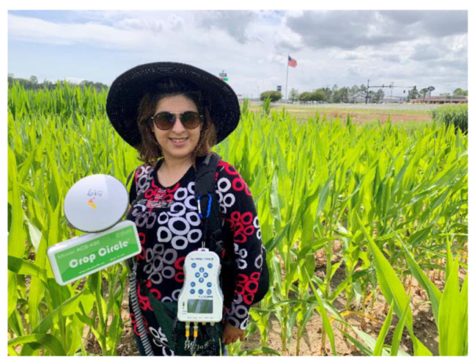
2.2. Data Collection

A Crop Circle ACS-430 (Holland Scientific Inc., Lincoln, NE, USA) was used in 2019 to collect canopy reflectance data at 670, 730, and 780 nm (red, red-edge, and NIR spectral bands) from rows 2 and 3 and rows 10 and 11 of each plot (Figure 1). Spectral reflectance data were simply and instantly recorded as a CSV file on a SD flash card using the Holland Scientific GeoSCOUT X datalogger (Figure 2). It also measured the NDVI and NDRE values directly with geolocation of each point 10 times per second (10 Hz). The sensor’s field of view was an oval of ~30 degrees by ~14 degrees. The sensor to canopy distance is suggested to be between 25 to 180 cm; however, in this research, the sensor was held at a consistent height of approximately 60 cm above the canopy, with a sampling speed of 10 Hz, while moving through each plot at a constant pace. The Crop Circle ACS-430 denotes reflectance measurements as Pseudo Solar Reflectance (PSR), which means the spectral reflectance wavelengths are scaled as percentages and will not differ in sensor height above a target [32]. The Crop Circle ACS-430 has an internal GPS to record the latitude, longitude, and elevation of each point, but it was not considered accurate enough for our purposes. Therefore, it was connected to a Piksi Multi Evaluation Kit (Swift Inc., Rocky View County, AB, Canada) as a Real-Time Kinematic (RTK) GPS. Data were extracted with a 3 m reduction from the starting edge and end of each plot length. This reduction was applied to skip the first and last crop canopy of each plot to eliminate border effects. Data were collected at three phenological stages (V4, V6, and VT) around 10:30 am. The average reflectance values were computed to represent rows 2, 3 and 10, 11 of each plot (Figure 1). The calculated spectral Vis, using red, red-edge, and NIR, are listed in

Table 1. Calculated spectral vegetation indices using red, red-edge, and NIR spectral bands.

	Vegetation Indices (VIs)	Abbreviation	Formula	Reference
1	Normalized Difference Vegetation Index	NDVI	(NIR − Red)/(NIR + Red)	[33]
2	Renormalized Difference Vegetation Index	RDVI	(NIR − Red)/$\sqrt{\mathrm{NIR}+\mathrm{Red}}$	[34]
3	Transformed Difference Vegetation Index	TDVI	1.5 × (NIR − Red)/$\sqrt{\mathrm{NIR}²+\mathrm{Red}+0.5}$	[35]
4	Difference Vegetation Index	DVI	NIR − Red	[36]
5	Red-edge difference vegetation index	REDVI	NIR − Red-edge	[36]
6	Red-edge re-normalized different vegetation index	RERDVI	(NIR − Red-edge)/$\sqrt{\mathrm{NIR}+\mathrm{Red}-\mathrm{edge}}$	[23]
7	Normalized Difference Red-edge	NDRE	(NIR − Red-edge)/(NIR + Red-edge)	[8,37]
8	Simplified Canopy Chlorophyll Content Index	SCCCI	NDRE/NDVI	[38]
9	Non-Linear Index	NLI	(NIR − Red)/(NIR2 + Red)	[39]
10	Modified Non-Linear Index	MNLI	(NIR − Red) × (1 + 0.5)/ (NIR2 + Red + 0.5)	[40] [41]
11	Soil Adjusted Vegetation Index	SAVI	1.5 × (NIR − Red)/(NIR + Red + 0.5)	[42]
12	Optimized Soil Adjusted Vegetation Index	OSAVI	(NIR − Red)/(NIR + Red + 0.16)	[42]
13	Modified Soil Adjusted Vegetation Index 2	MSAVI2	(2NIR + 1 − $\sqrt{{\left(2\mathrm{NIR}+1\right)}^2-8\left(\mathrm{NIR}-\mathrm{Red}\right)}$)/2	[43]
14	Simple Ratio	SR	NIR/Red	[44]
15	Modified Simple Ratio	MSR	(NIR/Red) − 1/$\sqrt{\left(\mathrm{NIR} /\mathrm{Red}\right)+1}$	[45]
16	Wide Dynamic Range Vegetation Index	WDRVI	(0.1 NIR − Red)/(0.1 NIR + Red)	[46]
17	Red-edge wide dynamic range vegetation index	REWDRVI	(0.12 × NIR − Red-edge)/(0.12 × NIR + Red-edge)	[23]
18	Red-edge ratio vegetation index	RERVI	NIR/Red-edge	[36]
19	Red-edge difference vegetation index	REDVI	NIR − Red-edge	[36]
20	Red-edge chlorophyll index	CIRE	(NIR/Red-edge) − 1	[47]
21	Modified red-edge simple ratio	MSR_RE	((NIR/Red-edge) – 1) /$\sqrt{\left(\mathrm{NIR}/\mathrm{Red}-\mathrm{edge}\right)+1}$	[23]
22	Red-edge soil adjusted vegetation index	RESAVI	1.5 × [(NIR − Red-edge)/(NIR + Red-edge + 0.5)]	[23]
23	Modified RESAVI	MRESAVI	0.5 × [2 * NIR + 1 − $\sqrt{\left(2\times \mathrm{NIR} +1\right)²-8\times \left(\mathrm{NIR} - \mathrm{Red}-\mathrm{edge}\right)}$ ]	[23]
24	Red-edge optimal soil adjusted vegetation index	REOSAVI	1.16 × (NIR − Red-edge)/(NIR + Red-edge + 0.16)	[23]
25	Red-edge re-normalized different vegetation index	RERDVI	(NIR − Red-edge)/$\sqrt{\mathrm{NIR} + \mathrm{Red}-\mathrm{edge}}$	[23]

.

2.2.1. Leaf Nitrogen Sampling

Whole plant or leaf samples were collected in 3 stages. Whole plant samples were collected at V4 stage (23 May 2019), leaf samples were taken at V6 (30 May 2019), and just before tassel emergence (VT) (21 June 2019). Six samples were collected from rows 2 and 3 and six samples from rows 10 and 11 (three samples from each row). The most recently matured and fully collared leaf of the individual corn plants were selected for sampling. Samples were placed in a forced-air oven and dried at 65 °C and weighed before they were ground through a 40-mesh sieve in a Wiley Mill and placed in airtight plastic vials. Again, they were dried at 65 °C and stored in sealed polypropylene vials until analysis and were processed for total N concentration on a Carlo Erba N/C 1500 automated dry combustion analyzer (Carlo Erba, Milan, Italy).

2.2.2. Grain Yield

The corn grain was harvested with a two-row plot combine for the entire plot length and grain yield was calculated on ton/ha for rows 2 and 3 and rows 10 and 11 of each plot (Figure 1). Grain yield was adjusted to a moisture content of 15.5%.

2.3. Statistical Analysis

2.3.1. Feature Selection

To remove irrelevant and redundant features, we were required to select the VIs that contributed most to predicting the target variable. Using irrelevant VIs can decrease the accuracy in the models; therefore, among the large number of VIs, we selected those that can optimally predict crop yield and plant tissue N concentration. There are different methods for feature selection such as a Univariate Selection ANOVA F-test, Principal Component Analysis, Recursive Feature Elimination (RFE), and bagged decision trees such as Random Forest (RF). For this study, RFE method [48], which is a popular feature selection method, was used to select predictors from the training data set that are more effective in predicting the independent variable and maximizing model accuracy. This method recursively removes attributes and builds the model on the remain features and works mainly in three steps including:

1-

RFE builds a model and estimates the feature importance by using a training data set.

2-

RFE sets the priority of the important features. It takes a subgroup of the selected variables in step 1 and builds models of a given subset size. In each iteration, the ranking of each feature is recalculated. In this step, the repeated cross-validations were implemented within the RFE method.

3-

The model performance is evaluated across different subset sizes to derive an optimal list of predictors.

Most importantly, the flexibility of this method in terms of the hyperparameters and the ability to control which algorithms are utilized, makes it an appropriate feature selection model for most ML applications. Since we were interested in fitting an appropriate model with a limited number of predictors, the RFE method was selected as it chooses the optimum number of features without affecting the model accuracy.

2.3.2. Machine Learning Methods

Since the observed grain yield and leaf N concentration data did not follow a normal distribution and the VIs and multispectral observation were highly correlated, this type of study is best analyzed through nonparametric models; therefore, this project utilized four nonparametric ML models to develop corn-leaf N concentration and grain yield prediction models. Four ML methods (RF, Gradient Boosting Model (GBM), Extreme Gradient Boosting (XGBoost), and Support Vector Regression (SVR)) were used in this study to find the best model to predict grain yield and the leaf N concentration of corn.

With its in-built ensemble capacity, Rf. [49] provides one of the most versatile ML algorithms, which is used for either regression or classification problems. This technique proves to be robust for correlated predictors, such as spectral bands or different VIs, and is used to solve both supervised and unsupervised ML problems. Random Forest models can provide variable interaction detection, nonlinear relationship detection, can handle missing values, and model local effects. However, one of the disadvantages of the Random Forest ML is that it tends to return erratic prediction in the case where observations are out of range of training data. Therefore, to come up with a robust prediction model, the training set should include the range of values at least as large as those that will be encountered when the model is tested.

Similarly, the GBM [50,51] is an RF model in that it runs numerous decision trees and uses these trees to compute an average. The GBM is a sequential modeling approach, though, the value added by this model is that each step learns from the previous step, whereas, with an RF model, all trees are run separately, and they do not learn from each other. In the GBM model, on the other hand, high residuals from one step are upweighted when they are fed into the next step, as a result, each tree can learn from previous trees.

The other model used in this research was the XGBoost [52]. This model is an optimized distributed algorithm that has recently dominated applied ML competitions for structured or tabular data. It has a fast and accurate performance for regression and classification. It also can prevent overfitting by adding a regularization term [53].

The regression model of Support Vector Machine [54,55], called Support Vector Regression (SVR), is a supervised-learning approach to predict continuous variables. This model is used to model linear and nonlinear relationships and the essential data points are chosen to solve the regression function. One of the advantages of SVR is that it is robust to the outliers and generalizing capability with high prediction accuracy [56].

The data set was randomly split into the training (75%) and testing (25%) set. Since this stage was used as an input feature in the ML models, in order to balance the datasets at each stage, a stratification approach was used to split data in a way that retains the same proportion of samples in each stage as observed in the original data set. Then, repeated cross validation (RCV) was used to train the models. In order to perform RCV, the training data set divided randomly into n folds and using each fold as testing data, the model trained on the rest of the n-1 folds. In RCV strategy we repeated this step several times (5 times in this study). The evaluations metrics illustrate the average of errors obtained when performing the RCV method. Since each repeat was randomly split the data into n-fold, the training-testing data in the first iteration of RCV are different than for the second iteration. Determining the optimal parameters of the ML models is critical for the bias-reduced assessment of a model’s predictive power. Therefore, hyperparameters tuning performed for each model by a set of parameters. Schematic of the tuning and cross validation procedure was as below:

Two groups of features were used to train the ML models including spectral bands and VIs. Growth stages was imported as inputs in both groups. Therefore, two strategies were used to train the N and yield prediction models. In the first method, ML models were trained based on spectral bands. In this step, four features, including Red, NIR, Red-edge, and growth stages were used as inputs in the training models. In the second strategy, the VIs selected by the RFE method and growth stages were used as input features for the training models. To add a threshold to the number of predictors in the RFE method, different set of the VIs (2, 3, 4, 5, 6, etc.) selected manually and the accuracy of the trained models compared with each other. If increasing the threshold did not substantially improve the accuracy of the model, least number of VIs was used.

Three statistical evaluation metrics, including mean absolute error (MAE), root mean square error (RMSE), and coefficient of determination (R²) were used to evaluate the performance of the ML models. The statistical R software (version 3.5) was employed to perform all statistical analyses and ML modeling in this research and the significance levels were indicated as follows: . = p-value < 0.1, * = p-value < 0.05, ** = p-value < 0.01, and *** = p-value < 0.001.

3. Results and Discussion

Among the several variables than can be used as inputs in ML modes, the RFE method selected SCCCI and RERVI, which are red-edge-based VIs [30,39,57,58,59,60] as predictors for estimating leaf N% and SCCCI, CIRE, RERVI, SAVI, and NDVI were chosen for predicting corn grain yield. Erdle et al. (2011) and Cao et al. (2013) found that RERVI was the most influential and temporally stable index for estimating leaf N concentration [23,61]. Bronson1 et al. (2020), compared the ability of 12 VIs to detect N deficiency between N treatments in irrigated cotton. They recommended the use of active canopy sensors with NIR and red-edge wavelength for N management of irrigated cotton under an overhead sprinkler irrigation system [62]. Besides, growth stages have a considerable effect on performing VIs for estimating plants biophysical parameters [12,24,63,64,65] and in this study, growth stage was imported to the models as an input for both leaf N estimation and yield prediction.

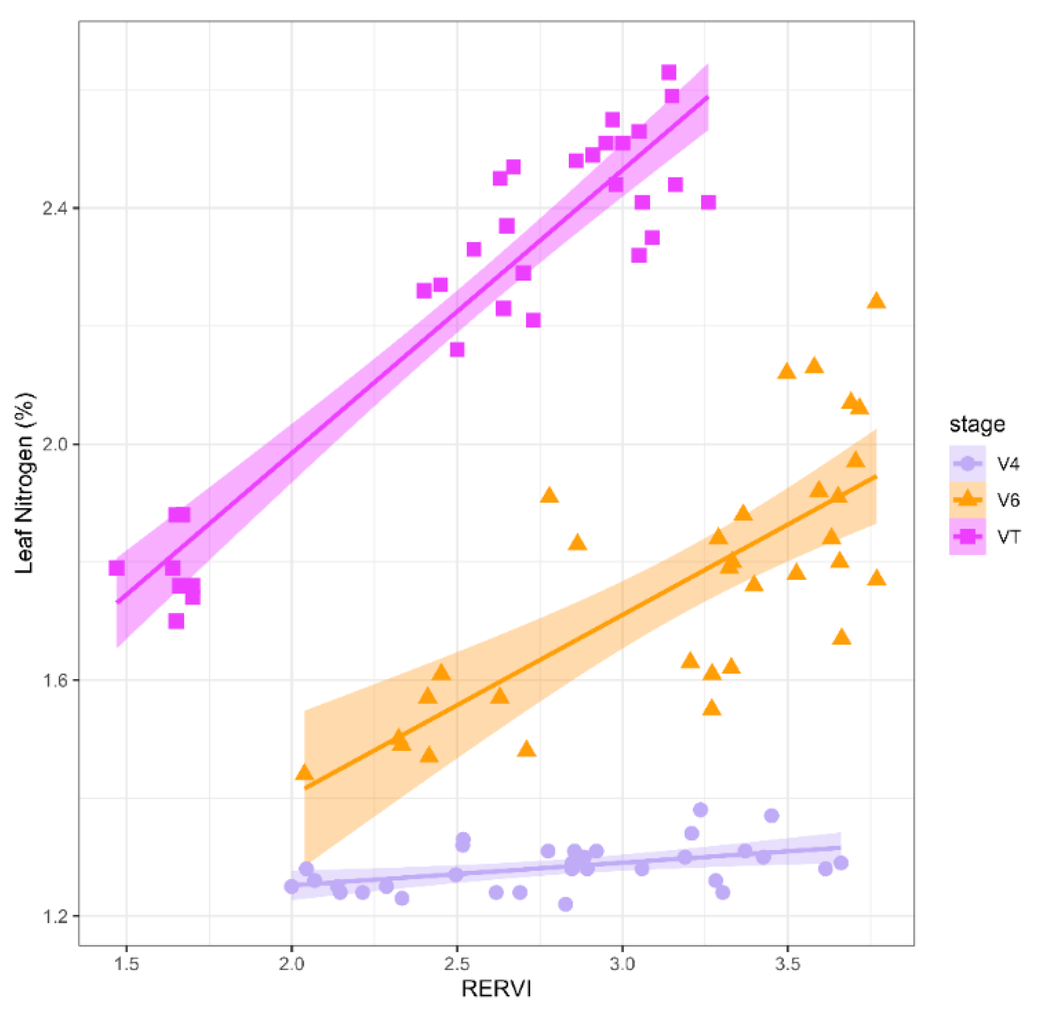
3.1. Regression Analysis

A comparison of the relationship between the SCCCI and RERVI with leaf N concentration and grain yield is presented in Figure 3. The data are organized in relation to the three phenological stages, including V4 (purple), V6 (orange), and VT (pink). The density plots illustrate the distribution of leaf N% as a response and SCCCI and RERVI as valid predictors of estimating leaf N%. The density plots for leaf N% (Figure 3, upper left) demonstrate that tissue N% does not follow the normal distribution at any of the growth stages. It has a similar probability distribution pattern for VIs at different phenological stages. For example, as shown in Figure 3, the SCCCI resulted in a near multimodal distribution. Scatter plots (lower panel) and associated correlations (upper panel) illustrated the relationships between the response variables (grain yield and leaf N%) and two independent variables (RERVI and SCCCI) for the three growth stages. Regarding the SCCCI index, the correlation coefficients between this index and leaf N% were −0.35, 0.90, and 0.92 at V4, V6, and VT stages, respectively. Correspondingly, the correlation coefficients between the RERVI and N were 0.48, 0.74, and 0.95 at the V4, V6, and VT stages, respectively. The correlation coefficients between grain yield and SCCCI were −0.44, 0.72, and 0.93 and between the yield and RERVI, they were 0.67, 0.79, and 0.97 for V4, V6, and VT, respectively. The correlation coefficients between SCCCI and others were negative at V4, which may have been the result of small corn plant size and high soil reflectance. Four histograms were associated with each phenological stage, and each variable is shown at the bottom of this figure. The boxplots in Figure 3 show the variability of measurements at each of the different growth stages. For example, as corn development progressed, average leaf N% increased (around 0.25%) from V4 to V6, then at the VT stage, it decreased to almost the same level as the V4 stage. A variation in RERVI was observed as the phenological stages changed from V6 to VT; however, unlike the SCCCI, a trend was observed at each growth stage. As illustrated in the scatterplot between RERVI and leaf N%, the variability in RERVI for each growth stage was independent of the other stages; therefore, separate regression models were fitted for each stage individually (Figure 4). Shen et al. (2014) reported that RERVI had a consistently greater correlation with plant N uptake across different growth stages [66]. The results of the regression analysis are illustrated in

Table 2. Linear regression results of leaf N (%) and RERVI. ** = p-value < 0.01, and *** = p-value < 0.001.

Stage	Residual Standard Error	R2	p-Value
V4	0.44	0.23	0.006 **
V6	0.36	0.54	1.45 $\times$ 10−6 ***
VT	0.19	0.89	5.8 $\times$ 10−16 ***

and the fitted lines are shown in Figure 4.

The regression analysis was performed for other VIs to evaluate the relationships between leaf N concentration and VIs. The preliminary results of the regression analysis were used to assess the importance of independent variables in the estimation of leaf N concentration. As illustrated in Table 2, RERVI had a statistically significant relationship with leaf N concentration at all three stages (all the p-values were less than 0.05 in 5% confidence interval).

3.2. Machine Learning Results

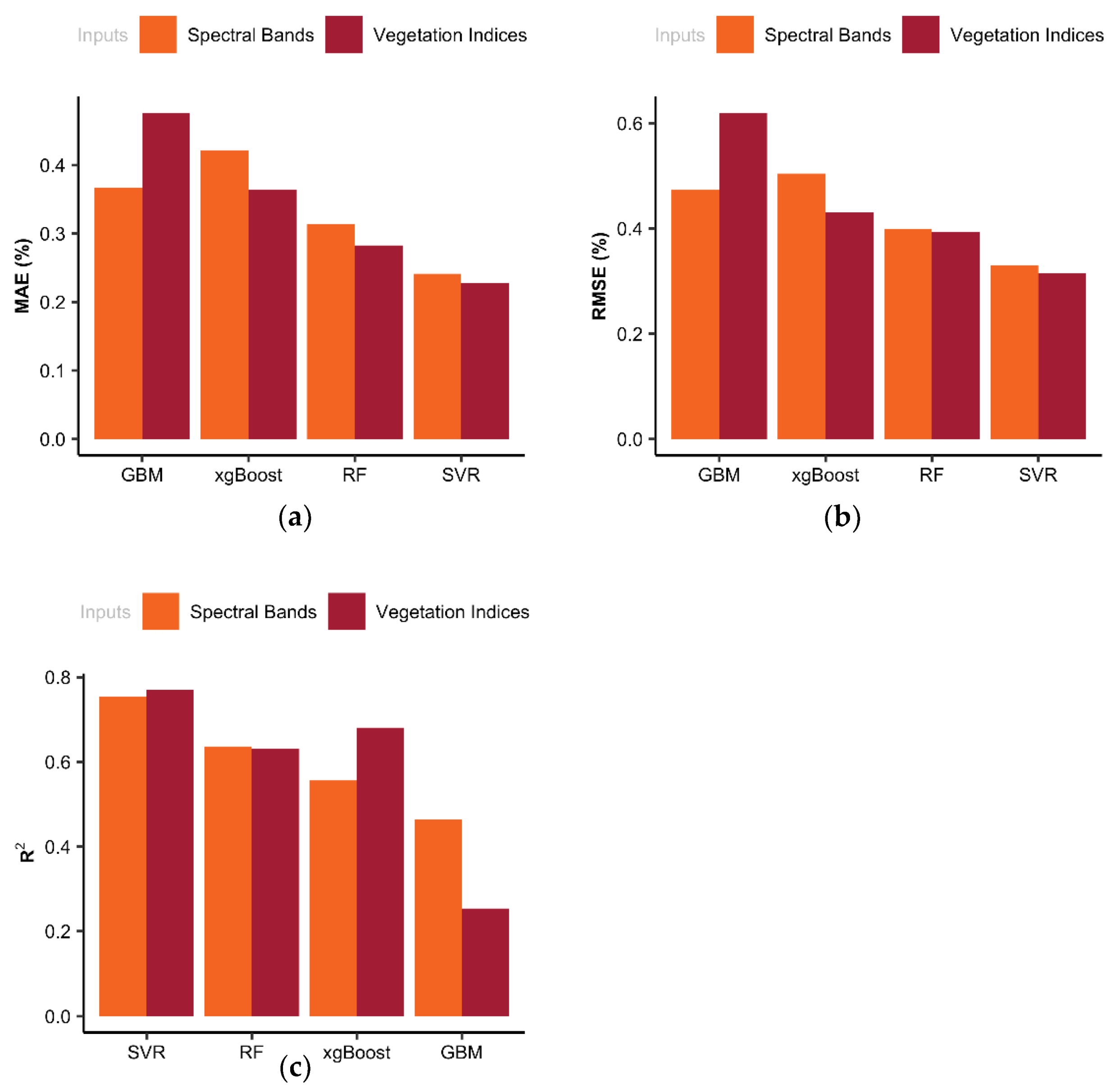
3.2.1. Machine Learning Results for N Estimation

The box plots in Figure 5 display the variation in mean absolute error (a), root mean square error (b), and R-squares (c) resulting from the cross-validation of training models. Two groups of box plots are shown in Figure 5, in which the orange plots show the cross-validation results derived from the ML model, which were trained by the VIs, and the brown plots illustrate the cross-validation results derived from the models, which were trained by the spectral raw data. In this study, four non-parametric ML models were used to estimate the leaf N concentration. As indicated in Figure 5, the evaluation metrics were different for all models. For example, in the wavelength-based models, the average R² values resulting from cross-validations in the training data set were 0.61, 0.48, 0.62, and 0.75 for RF, XGBoost, GBM, and SVR models, respectively. The results indicated that SVR model had the least MAE and RMSE, and the greatest R², therefore it can be concluded that the SVR model outperformed the other models in almost all performance measures. As illustrated, the SVR model could explain approximately 75% of the variability of N content using wavelength-based inputs. Cummings et al., 2021, evaluated Crop Circle Phenom for in-season diagnosis of corn N status during two years’ growing season in Minnesota, United States. Their results showed that Canopy Chlorophyll Content Index (CCCI) was an important vegetation index for predicting plant N concentration and plant N uptake in both simple regression (SR) and XGB modeling [67].

Overall, a comparison of the performance of two groups of ML models indicated that the models trained by the VIs had slightly greater accuracy in comparison to models trained by the spectral bands in N prediction. According to these results, we can conclude that the ML models can manage the linear and non-linear relationships between the input features (i.e., spectral bands). The results of this study ranked the ML leaf N% estimation models from the best to the worst, according to the statistical evaluation metrics in the following order: SVR, RF, GBM, and XGBoost. In addition, regarding the performance of the ML models, the same order was observed for both VI-based and wavelength-based modeling approaches.

The performance of well-trained models was evaluated using the test data (25% of the samples), that did not contribute to training the models. As illustrated in Figure 6, the SVR model had achieved the best performance measures as compared to the other models. As a result, this study illustrated that either spectral bands or VIs derived from the Crop Circle sensor can be used as reliable inputs for the SVR model to predict corn leaf N% accurately. Bakar et al. 2021, investigated instantaneous fertilizer application for rice using a Crop Circle ACS-430. They applied SVR on spectral data and vegetation indices to develop a crop N status prediction model. The model was then incorporated into a practical on-the-go variable rate application system. Their results demonstrated that the model had an 83% accuracy in classifying the N status of the plants and was able to save up to 20% fertilizer use while maintaining yield [68]. The observed leaf N values varied between 1.47% through 3.77% and the average was 2.8%. The mean absolute values in Figure 5 and Figure 6 indicated that the fitted SVR model can estimate the leaf N content with an absolute error of 0.26% on average. For instance, if the leaf N content in an un-seen leaf was about 2%, the model can estimate it between 1.74% and 2.26%. Moreover, the Mean Absolute Percentage Error (MAPE), which is commonly used to measure the predictive accuracy of models, of the SVR model was 4.4%, indicating that the average difference between the predicted value and the actual value was 4.4%. The MAPE was 6.4%, 6.5%, and 7.7% for RF, xgBoost, and GBM, respectively.

Figure 7 indicates the observed and predicted leaf N content using the testing data set. The result indicated the performance of the well-trained models, which shows that the predicted values agree well with the observed data. In both modeling strategies, the SVR model had significantly enhanced performance in comparison to the other models. While it may be more difficult to interpret the non-parametric models such as RF, in addition to the SVR model, it was found to be a better predictor of corn leaf N concentration in this study.

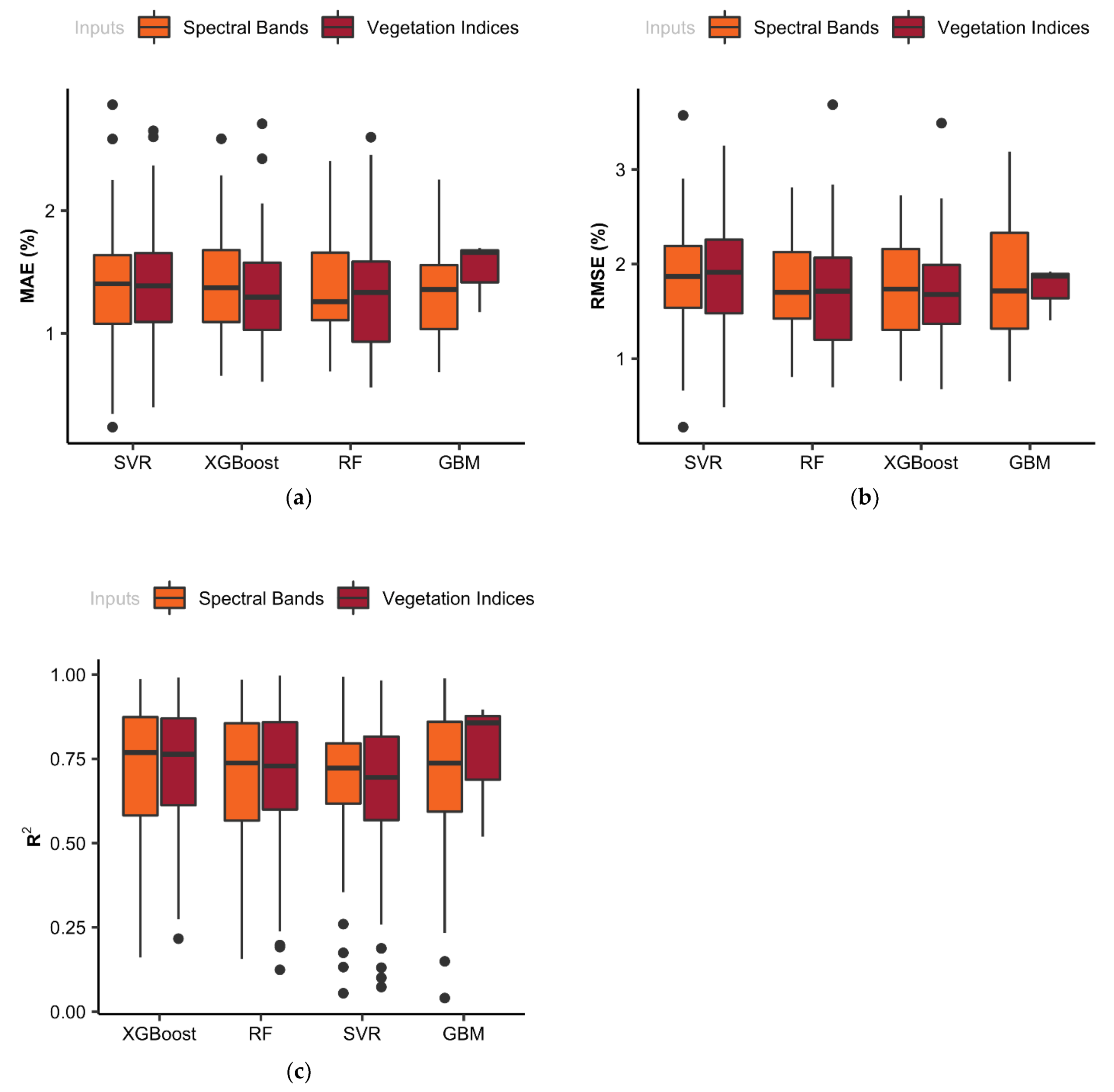
3.2.2. Machine Learning Results for Yield Estimation

The variation in MAE (a), RMSE (b), and R² (c) resulted from the cross-validation of the training models, as demonstrated in Figure 8. Regarding the wavelength-based models, the average R² values resulted from cross-validations in the training data set were 0.73, 0.76, 0.74, and 0.72 for RF, XGBoost, GBM, and SVR models, respectively. Results indicated that there was no dramatic difference between these models. The results of cross-validation showed that the first quartile, median, and third quartile were almost the same for all of the ML models, indicating that there was no major difference between these models (Figure 8).

Figure 9 indicates the observed and predicted grain yield using the testing data set. The points under the red line (1:1 line) indicate that the model underestimated grain yield and the points above the 1:1 line represent the overestimation. Good correspondence was found between the observed and predicted grain yield, indicating that well-trained models can predict the grain yield well.

4. Conclusions

This study was conducted to evaluate the reliability of a handheld Crop Circle ACS-430 in estimating corn leaf N% and predict grain yield corn using ML algorithms. The recursive feature elimination method was applied and determined that SCCCI and RERVI were the most effective VIs to estimate corn leaf N concentration. This method also determined that SCCCI, CI_RE, RERVI, SAVI, and NDVI were the most efficient VIs in predicting corn grain yield. Furthermore, between the four ML models utilized in this research, the SVR achieved the most accurate results for leaf N% estimation using either the spectral bands or VIs as the model inputs. Further evaluation would help to detect possible model-performance changes using improved inputs, model updates, or an increased number and quality of observations. More studies are required to further evaluate this sensor using a larger dataset collected across a wider and more varied range of environments.

References

1. West, P.C.; Gibbs, H.K.; Monfreda, C.; Wagner, J.; Barford, C.C.; Carpenter, S.R. Trading Carbon for Food: Global Comparison of Carbon Stocks vs. Crop Yields on Agricultural Land. Proc. Natl. Acad. Sci. USA 2010, 107, 19645–19648. [Google Scholar] [CrossRef] [PubMed] [Green Version]
2. McGuire, S. WHO, World Food Programme, and International Fund for Agricultural Development. 2012. The State of Food Insecurity in the World 2012. Economic Growth Is Necessary but Not Sufficient to Accelerate Reduction of Hunger and Malnutrition. Rome, FAO. Adv. Nutr. 2013, 4, 126–127. [Google Scholar] [CrossRef] [Green Version]
3. USDA. NASS_USAD.pdf. Available online: http://www.nass.usda.gov/Quick_Stats (accessed on 21 December 2021).
4. Andrews, M.; Raven, J.A.; Lea, P.J. Do Plants Need Nitrate? The Mechanisms by Which Nitrogen Form Affects Plants. Ann. Appl. Biol. 2013, 163, 174–199. [Google Scholar] [CrossRef]
5. Cassman, K.G.; Dobermann, A.; Walters, D.T.; Yang, H. Meeting Cereal Demand While Protecting Natural Resources and Improving Environmental Quality. Annu. Rev. Environ. Resour. 2003, 28, 315–358. [Google Scholar] [CrossRef] [Green Version]
6. Kim, S.; Dale, B.E. Effects of Nitrogen Fertilizer Application on Greenhouse Gas Emissions and Economics of Corn Production. Environ. Sci. Technol. 2008, 42, 6028–6033. [Google Scholar] [CrossRef] [PubMed]
7. Gautam, R.K.; Panigrahi, S. Leaf Nitrogen Determination of Corn Plant Using Aerial Images and Artificial Neural Networks. Can. Biosyst. Eng./Genie Biosyst. Can. 2007, 49, 9. [Google Scholar]
8. Raper, T.B.; Varco, J.J.; Hubbard, K.J. Canopy-Based Normalized Difference Vegetation Index Sensors for Monitoring Cotton Nitrogen Status. Agron. J. 2013, 105, 1345–1354. [Google Scholar] [CrossRef] [Green Version]
9. Bronson, K.F.; Booker, J.D.; Keeling, J.W.; Boman, R.K.; Wheeler, T.A.; Lascano, R.J.; Nichols, R.L. Cotton Canopy Reflectance at Landscape Scale as Affected by Nitrogen Fertilization. Agron. J. 2005, 97, 654–660. [Google Scholar] [CrossRef]
10. Fridgen, J.L.; Varco, J.J. Dependency of cotton leaf nitrogen, chlorophyll, and reflectance on nitrogen and potassium availability. Agron. J. 2004, 96, 63–69. [Google Scholar] [CrossRef]
11. Zhao, D.; Reddy, K.R.; Kakani, V.G.; Read, J.J.; Carter, G.A. Corn (Zea mays L.) Growth, Leaf Pigment Concentration, Photosynthesis and Leaf Hyperspectral Reflectance Properties as Affected by Nitrogen Supply. Plant Soil 2003, 257, 205–218. [Google Scholar] [CrossRef]
12. Li, F.; Miao, Y.; Hennig, S.D.; Gnyp, M.L.; Chen, X.; Jia, L.; Bareth, G. Evaluating Hyperspectral Vegetation Indices for Estimating Nitrogen Concentration of Winter Wheat at Different Growth Stages. Precis. Agric. 2010, 11, 335–357. [Google Scholar] [CrossRef]
13. Zhu, Y.; Fan, X.; Hou, X.; Wu, J.; Wang, T. ScienceDirect Effect of Different Levels of Nitrogen Deficiency on Switchgrass Seedling Growth. Crop. J. 2014, 2, 223–234. [Google Scholar] [CrossRef] [Green Version]
14. Reyniers, M.; Vrindts, E.; De Baerdemaeker, J. Comparison of an Aerial-Based System and an on the Ground Continuous Measuring Device to Predict Yield of Winter Wheat. Eur. J. Agron. 2006, 24, 87–94. [Google Scholar] [CrossRef]
15. Chang, J.; Clay, D.E.; Dalsted, K.; Clay, S.; O’Neill, M. Corn (Zea mays L.) Yield Prediction Using Multispectral and Multidate Reflectance. Agron. J. 2003, 95, 1447–1453. [Google Scholar] [CrossRef]
16. Solari, F.; Shanahan, J.; Ferguson, R.; Schepers, J.; Gitelson, A. Active Sensor Reflectance Measurements of Corn Nitrogen Status and Yield Potential. Agron. J. 2008, 100, 571–579. [Google Scholar] [CrossRef] [Green Version]
17. Tadesse, A.; Kim, H.K.; Debela, A. Calibration of Nitrogen Fertilizer for Quality Protein Maize (Zea mays L.) Based on In-Season Estimated Yield Using a Handheld NDVI Sensor in the Central. Asia Pac. J. Energy Environ. 2015, 2, 25–32. [Google Scholar] [CrossRef]
18. Sakamoto, T.; Gitelson, A.A.; Arkebauer, T.J. Near Real-Time Prediction of U.S. Corn Yields Based on Time-Series MODIS Data. Remote Sens. Environ. 2014, 147, 219–231. [Google Scholar] [CrossRef]
19. Uno, Y.; Prasher, S.O.; Lacroix, R.; Goel, P.K.; Karimi, Y.; Viau, A.; Patel, R.M. Artificial Neural Networks to Predict Corn Yield from Compact Airborne Spectrographic Imager Data. Comput. Electron. Agric. 2005, 47, 149–161. [Google Scholar] [CrossRef]
20. Dobermann, A.; Witt, C.; Dawe, D.; Abdulrachman, S.; Gines, H.C.; Nagarajan, R.; Satawathananont, S.; Son, T.T.; Tan, P.S.; Wang, G.H.; et al. Site-Specific Nutrient Management for Intensive Rice Cropping Systems in Asia. F. Crop. Res. 2002, 74, 37–66. [Google Scholar] [CrossRef]
21. Gitelson, A.A.; Merzlyak, M.N. Remote Estimation of Chlorophyll Content in Higher Plant Leaves. Int. J. Remote Sens. 1998, 18, 2691–2697. [Google Scholar] [CrossRef]
22. Yao, Y.; Miao, Y.; Huang, S.; Gao, L.; Ma, X.; Zhao, G.; Jiang, R.; Chen, X.; Zhang, F.; Yu, K.; et al. Active Canopy Sensor-Based Precision N Management Strategy for Rice. Agron. Sustain. Dev. 2012, 32, 925–933. [Google Scholar] [CrossRef] [Green Version]
23. Cao, Q.; Miao, Y.; Wang, H.; Huang, S.; Cheng, S.; Khosla, R.; Jiang, R. Non-Destructive Estimation of Rice Plant Nitrogen Status with Crop Circle Multispectral Active Canopy Sensor. F. Crop. Res. 2013, 154, 133–144. [Google Scholar] [CrossRef]
24. Hatfield, J.L.; Prueger, J.H. Value of Using Different Vegetative Indices to Quantify Agricultural Crop Characteristics at Different Growth Stages under Varying Management Practices. Remote Sens. 2010, 2, 562–578. [Google Scholar] [CrossRef] [Green Version]
25. Cao, Q.; Miao, Y.; Li, F.; Gao, X. Developing a New Crop Circle Active Canopy Sensor- Based Precision Nitrogen Management Strategy for Winter. Precis. Agric. 2017, 18, 2–18. [Google Scholar] [CrossRef]
26. Shi, W.; Lu, J.; Miao, Y.; Cao, Q.; Shen, J.; Wang, H.; Hu, X.; Hu, S. Evaluating a Crop Circle Active Canopy Sensor-Based Precision Nitrogen Management Strategy for Rice in Northeast China. In Proceedings of the 2015 Fourth International Conference on Agro-Geoinformatics (Agro-geoinformatics), Istanbul, Turkey, 20–24 July 2015; pp. 261–264. [Google Scholar] [CrossRef]
27. Wahabzada, M.; Mahlein, A.; Bauckhage, C.; Steiner, U. Plant Phenotyping Using Probabilistic Topic Models: Uncovering the Hyperspectral Language of Plants. Nat. Publ. Gr. 2016, 6, 22482. [Google Scholar] [CrossRef] [PubMed] [Green Version]
28. Goldstein, A.; Fink, L.; Meitin, A. Applying Machine Learning on Sensor Data for Irrigation Recommendations: Revealing the Agronomist’ s Tacit Knowledge. Precis. Agric. 2017, 19, 421–444. [Google Scholar] [CrossRef]
29. Barzin, R.; Pathak, R.; Lotfi, H.; Varco, J.; Bora, G.C. Use of UAS Multispectral Imagery at Different Physiological Stages for Yield Prediction and Input Resource Optimization in Corn. Remote. Sens. 2020, 12, 2392. [Google Scholar] [CrossRef]
30. Gutiérrez, S.; Diago, M.P.; Fernández-Novales, J.; Tardaguila, J. Vineyard Water Status Assessment Using On-the-Go Thermal Imaging and Machine Learning. PLoS ONE 2018, 13, e0192037. [Google Scholar] [CrossRef]
31. Weng, H.; Lv, J.; Cen, H.; He, M.; Zeng, Y.; Hua, S.; Li, H.; Meng, Y.; Fang, H.; He, Y. Hyperspectral Re Fl Ectance Imaging Combined with Carbohydrate Metabolism Analysis for Diagnosis of Citrus Huanglongbing in Di Ff Erent Seasons and Cultivars. Sensors Actuators B. Chem. 2018, 275, 50–60. [Google Scholar] [CrossRef]
32. Cao, Q.; Miao, Y.; Shen, J.; Yuan, F.; Cheng, S.; Cui, Z. Evaluating Two Crop Circle Active Canopy Sensors for In-Season Diagnosis of Winter Wheat. Agronomy 2018, 8, 201. [Google Scholar] [CrossRef] [Green Version]
33. Rouse, J.W.; Hass, R.H.; Schell, J.A.; Deering, D.W.; Harlan, J.C. Monitoring the Vernal Advancement and Retrogradation (GreenWave Effect) of Natural Vegetation; NASA: Greenbelt, MD, USA, 1974. [Google Scholar]
34. Roujean, J.L.; Breon, F.M. Estimating PAR Absorbed by Vegetation from Bidirectional Reflectance Measurements. Remote Sens. Environ. 1995, 51, 375–384. [Google Scholar] [CrossRef]
35. Bannari, A.; Asalhi, H.; Teillet, P.M. Transformed Difference Vegetation Index (TDVI) for Vegetation Cover Mapping. IEEE Int. Geosci. Remote Sens. Symp. 2002, 5, 3053–3055. [Google Scholar] [CrossRef]
36. Tucker, C.J. Red and Photographic Infrared Linear Combinations for Monitoring Vegetation. Remote Sens. Environ. 1979, 8, 127–150. [Google Scholar] [CrossRef] [Green Version]
37. Gitelson, A.A.; Merzlyak, M.N. Quantitative Estimation of Chlorophyll-a Using Reflectance Spectra: Experiments with Autumn Chestnut and Maple Leaves. J. Photochem. Photobiol. 1994, 22, 247–252. [Google Scholar] [CrossRef]
38. Raper, T.B.; Varco, J.J. Canopy-Scale Wavelength and Vegetative Index Sensitivities to Cotton Growth Parameters and Nitrogen Status. Precis. Agric. 2015, 16, 62–76. [Google Scholar] [CrossRef] [Green Version]
39. Vescovo, L.; Gianelle, D. Using the MIR Bands in Vegetation Indices for the Estimation of Grassland Biophysical Parameters from Satellite Remote Sensing in the Alps Region of Trentino (Italy). Adv. Sp. Res. 2008, 41, 1764–1772. [Google Scholar] [CrossRef]
40. Gong, P.; Pu, R.; Biging, G.S.; Larrieu, M.R. Estimation of Forest Leaf Area Index Using Vegetation Indices Derived from Hyperion Hyperspectral Data. IEEE Trans. Geosci. Remote Sens. 2003, 41, 1355–1362. [Google Scholar] [CrossRef] [Green Version]
41. Feng, W.; Wu, Y.; He, L.; Ren, X.; Wang, Y.; Hou, G.; Wang, Y.; Liu, W.; Guo, T. An Optimized Non-Linear Vegetation Index for Estimating Leaf Area Index in Winter Wheat. Precis. Agric. 2019, 20, 1157–1176. [Google Scholar] [CrossRef] [Green Version]
42. Rondeaux, G.; Steven, M.; Baret, F. Optimization of Soil-Adjusted Vegetation Indices. Remote Sens. Environ. 1996, 55, 95–107. [Google Scholar] [CrossRef]
43. Qi, J.; Chehbouni, A.; Huete, A.R.; Kerr, Y.H.; Sorooshian, S. A Modify Soil Adjust Vegetation Index. Remote Sens. Environ. 1994, 126, 119–126. [Google Scholar] [CrossRef]
44. Fraser, R.H.; Latifovic, R. Mapping Insect-Induced Tree Defoliation and Mortality Using Coarse Spatial Resolution Satellite Imagery. Int. J. Remote Sens. 2005, 26, 193–200. [Google Scholar] [CrossRef]
45. Chen, J.M. Evaluation of Vegetation Indices and a Modified Simple Ratio for Boreal Applications. Can. J. Remote Sens. 1996, 22, 229–242. [Google Scholar] [CrossRef]
46. Gitelson, A.A. Wide Dynamic Range Vegetation Index for Remote Quantification of Biophysical Characteristics of Vegetation. J. Plant Physiol. 2004, 161, 165–173. [Google Scholar] [CrossRef] [Green Version]
47. Gitelson, A.A.; Viña, A.; Ciganda, V.; Rundquist, D.C.; Arkebauer, T.J. Remote Estimation of Canopy Chlorophyll Content in Crops. Geophys. Res. Lett. 2005, 32, 7. [Google Scholar] [CrossRef] [Green Version]
48. Granitto, P.M.; Furlanello, C.; Biasioli, F.; Gasperi, F. Recursive Feature Elimination with Random Forest for PTR-MS Analysis of Agroindustrial Products. Chemom. Intell. Lab. Syst. 2006, 83, 83–90. [Google Scholar] [CrossRef]
49. Breiman, L. Random Forests. Mach. Learn. 2001, 45, 5–32. [Google Scholar] [CrossRef] [Green Version]
50. Natekin, A.; Knoll, A. Gradient Boosting Machines, a Tutorial. Front. Neurorobotics 2013, 7, 21. [Google Scholar] [CrossRef] [Green Version]
51. Friedman, J.H. Stochastic Gradient Boosting. Comput. Stat. Data Anal. 2002, 38, 367–378. [Google Scholar] [CrossRef]
52. Chen, T.; Guestrin, C. XGBoost: A Scalable Tree Boosting System. In Proceedings of the 22nd ACM SIGKDD International Conference on Knowledge Discovery and Data Mining, San Francisco, CA, USA, 13–17 August 2016; pp. 785–794. [Google Scholar] [CrossRef]
53. Mo, H.; Sun, H.; Liu, J.; Wei, S. Developing Window Behavior Models for Residential Buildings Using XGBoost Algorithm. Energy Build 2019, 205, 109564. [Google Scholar] [CrossRef]
54. Vapnik, V.; Golowich, S.E.; Ave, M.; Hill, M. Support Vector Method for Function Approximation, Regression Estimation, and Signal Processing. Adv. Neural Inf. Process. Syst. 1997, 20, 281–287. [Google Scholar]
55. Vapnik, V. The Support Vector Method of Function Estimation. In Nonlinear Modeling; Springer: Boston, MA, USA, 1998; pp. 55–85. [Google Scholar]
56. Awad, M.; Khanna, R. Efficient Learning Machines: Theories, Concepts, and Applications for Engineers and System Designers; Apress: New York, NY, USA, 2015. [Google Scholar]
57. Sumner, Z. Multi-Platform Comparison of Canopy Reflectance on Corn Whole Plant and Leaf Tissue Nitrogen Status. Ph.D. Thesis, Mississippi State University, Starkville, MS, USA, 2019. [Google Scholar]
58. Fox, A.A.A. An Integrated Approach for Predicting Nitrogen Status in Early Cotton and Corn. Ph.D. Thesis, Mississippi State University, Starkville, MS, USA, 2015. [Google Scholar]
59. Sumner, Z.; Varco, J.J.; Dhillon, J.S.; Fox, A.A.A.; Czarnecki, J.; Henry, W.B. Ground versus Aerial Canopy Reflectance of Corn: Red-Edge and Non-Red Edge Vegetation Indices. Agron. J. 2021, 113, 2773–2788. [Google Scholar] [CrossRef]
60. Barzin, R.; Kamangir, H.; Bora, G.C. Comparison of Machine Learning Methods for Leaf Nitrogen Estimation in Corn Using Multispectral UAV images. Trans. ASABE 2021, 64, 2089–2101. [Google Scholar] [CrossRef]
61. Erdle, K.; Mistele, B.; Schmidhalter, U. Field Crops Research Comparison of Active and Passive Spectral Sensors in Discriminating Biomass Parameters and Nitrogen Status in Wheat Cultivars. Field Crop. Res. 2011, 124, 74–84. [Google Scholar] [CrossRef]
62. Bronson, K.F.; Conley, M.M.; French, A.N.; Hunsaker, D.J.; Thorp, K.R.; Barnes, E.M. Which active optical sensor vegetation index is best for nitrogen assessment in irrigated cotton? Agron. J. 2020, 112, 2205–2218. [Google Scholar] [CrossRef]
63. Miao, Y.; Mulla, D.J.; Randall, G.W.; Vetsch, J.A.; Vintila, R. Combining Chlorophyll Meter Readings and High Spatial Resolution Remote Sensing Images for In-Season Site-Specific Nitrogen Management of Corn. Precis. Agric. 2008, 10, 45–62. [Google Scholar] [CrossRef]
64. Li, F.; Mistele, B.; Hu, Y.; Yue, X.; Yue, S.; Miao, Y.; Chen, X.; Cui, Z.; Meng, Q.; Schmidhalter, U. Remotely Estimating Aerial N Status of Phenologically Differing Winter Wheat Cultivars Grown in Contrasting Climatic and Geographic Zones in China and Germany. Field Crop. Res. 2012, 138, 21–32. [Google Scholar] [CrossRef]
65. Yu, K.; Li, F.; Gnyp, M.L.; Miao, Y.; Bareth, G.; Chen, X. Remotely Detecting Canopy Nitrogen Concentration and Uptake of Paddy Rice in the Northeast China Plain. ISPRS J. Photogramm. Remote Sens. 2013, 78, 102–115. [Google Scholar] [CrossRef]
66. Shen, J.; Miao, Y.; Cao, Q.; Wang, H.; Yu, W.; Hu, S.; Wu, H.; Lu, J. Estimating Rice Nitrogen Status Using Active Canopy Sensor Crop Circle 430 in Northeast China. In Proceedings of the Third International Conference on Agro-Geoinformatics, Beijing, China, 11–14 August 2014; pp. 1–7. [Google Scholar] [CrossRef]
67. Cummings, C.; Miao, Y.; Paiao, G.D.; Kang, S.; Fernández, F.G. Corn nitrogen status diagnosis with an innovative multi-parameter crop circle phenom sensing system. Remote Sens. 2021, 13, 401. [Google Scholar] [CrossRef]
68. Bakar, B.A.; Muslimin, J.; Rani, M.N.F.A.; Bookeri, M.A.M.; Ahmad, M.T.; Abdullah, M.Z.K.; Ismail, R. On-The-Go Variable Rate Fertilizer Application Method for Rice Through Classification of Crop Nitrogen Nutrition Index (NNI). ASM Sci. J. 2021, 15, 1–10. [Google Scholar] [CrossRef]
Figure 1. Fertilizer Nitrogen (N) treatments and 4 replicates for corn in 2019 at Agriculture Systems Research Farm, Mississippi State, USA.
Remotesensing 14 00120 g001
Figure 2. Crop Circle ACS-430 and GeoSCOUT X datalogger connected to RTK GPS.
Remotesensing 14 00120 g002
Figure 3. Exploratory data analysis for N, yield, RERVI, and SCCCI at different phenological stages. The significance levels were as follows: . = p-value < 0.1, * = p-value < 0.05, ** = p-value < 0.01, and *** = p-value < 0.001.
Remotesensing 14 00120 g003
Figure 4. Scatter plots of RERVI versus leaf N percent in different corn growth stages.
Remotesensing 14 00120 g004
Figure 5. Statistical evaluation metrics including (a) mean absolute error (MAE), (b) root mean square error (RMSE), and (c) coefficient of determination (R2) resulted from cross-validation in two sets of machine learning models to estimate leaf N content.
Remotesensing 14 00120 g005
Figure 6. Statistical evaluation metrics including (a) mean absolute error (MAE), (b) root mean square error (RMSE), and (c) coefficient of determination (R2) derived from ML models’ performance on the validation (test) data set for leaf N% prediction.
Remotesensing 14 00120 g006
Figure 7. Scatter plot of observed vs. predicted leaf N content using VIs to evaluate SVR model’s performance on the test data.
Remotesensing 14 00120 g007
Figure 8. Statistical evaluation metrics including (a) mean absolute error (MAE), (b) root mean square error (RMSE), and (c) coefficient of determination (R2) resulted from cross-validation in two sets of ML models in order to estimate yield of corn.
Remotesensing 14 00120 g008
Figure 9. Scatter plot of observed vs. predicted grain yield using VIs to evaluate SVR model’s performance on the test data.
Remotesensing 14 00120 g009