
Grounding Event of Iceberg D28 and Its Interactions with Seabed Topography
by
 , , , and
Xuying Liu
1, 
Xiao Cheng
2,*,
Qi Liang
2,
Teng Li
2 ,
,
Fukai Peng
2,
Zhaohui Chi
3 and
Jiaying He
4 1
State Key Laboratory of Remote Sensing Science, College of Global Change and Earth System Science, Beijing Normal University, Beijing 100875, China
2
School of Geospatial Engineering and Science, Sun Yat-sen University & Southern Marine Science and Engineering Guangdong Laboratory (Zhuhai), Zhuhai 519082, China
3
Department of Geography, Texas A&M University, College Station, TX 77843, USA
4
Department of Earth System Science, Ministry of Education Key Laboratory for Earth System Modeling, Institute for Global Change Studies, Tsinghua University, Beijing 100084, China
*
Author to whom correspondence should be addressed.
Remote Sens. 2022, 14(1), 154; https://0-doi-org.brum.beds.ac.uk/10.3390/rs14010154
Submission received: 22 October 2021
/
Revised: 23 December 2021
/
Accepted: 27 December 2021
/
Published: 30 December 2021
(This article belongs to the Special Issue The Cryosphere Observations Based on Using Remote Sensing Techniques)
Abstract
:Iceberg D28, a giant tabular iceberg that calved from Amery Ice Shelf in September 2019, grounded off Kemp Coast, East Antarctica, from August to September of 2020. The motion of the iceberg is characterized herein by time-series images captured by synthetic aperture radar (SAR) on Sentinel-1 and the moderate resolution imaging spectroradiometer (MODIS) boarded on Terra from 6 August to 15 September 2020. The thickness of iceberg D28 was estimated by utilizing data from altimeters on Cryosat-2, Sentinel-3, and ICESat-2. By using the iceberg draft and grounding point locations inferred from its motion, the maximum water depths at grounding points were determined, varying from 221.72 ± 21.77 m to 269.42 ± 25.66 m. The largest disagreements in seabed elevation inferred from the grounded iceberg and terrain models from the Bedmap2 and BedMachine datasets were over 570 m and 350 m, respectively, indicating a more complicated submarine topography in the study area than that presented by the existing seabed terrain models. Wind and sea water velocities from reanalysis products imply that the driving force from sea water is a more dominant factor than the wind in propelling iceberg D28 during its grounding, which is consistent with previous findings on iceberg dynamics.

1. Introduction
Grounding is a common process during the life course of an iceberg. When an iceberg drifts into shallow water areas, its keel cuts into sediments; then, a grounding event occurs. The process can last from days to years [1,2], during which the iceberg scours on the seabed under multiple environmental factors, such as the Coriolis force, wind, and currents around it [3]. The scouring creates plough marks that can provide insight into oceanic and glaciological conditions, revealing ocean–ice interaction procedures [4,5,6]. Investigation of continental land shelves and submarine plateaus presents plow marks of mega icebergs in the Late Pleistocene age indicative of submarine landform processes [7]. A recent study implies that iceberg grounding can trigger submarine landslides on certain occasions and can become hazards to coastal regions thousands of kilometers away [8]. In addition to modifying submarine topography, grounded icebergs can damage benthic communities through their interactions with the seabed, supported by in situ observations of several benthic habitats in polar areas [9,10,11,12].
Environmental factors control the motion of grounded icebergs in ways similar to determining their drifting pattern, but with the constraints of seabed topography [2,3,13]. Dynamic models show that for most icebergs, the dominant forces are the water drag force and the horizontal gradient force exerted by the water displaced, contributing about 70 ± 15% of the total force [3]. The other 30% of the driving force is contributed by the Coriolis force and the air drag force together. However, for icebergs in certain areas, such as the Nares Strait between Ellesmere Island and Greenland, the air drag force is a more important factor than the water [3]. Further research on iceberg drifting models establishes the relationship between iceberg size and driving forces. Wind-driven iceberg motion is less than 10% of the ocean-driven motion for large icebergs with lengths larger than 12 km [13].
Studies on iceberg detection and evolution widely utilize remote sensing technology, especially radar and satellite altimetry [14,15,16,17,18,19,20,21]. Radar instruments can capture Earth’s surface regardless of cloud cover and polar night. Moreover, radar backscatter of icebergs is higher than that of surrounding sea ice or water throughout the year except in austral summer (December, January, and February), when melted water in snowpacks and firns can reduce the backscatter of icebergs [18,21]. Satellite altimeters are used to estimate the iceberg freeboard and thickness, especially on large icebergs. Studies of tabular icebergs, such as iceberg A68, C28, and B30, are carried out with data from the European Space Agency (ESA) Envisat Advanced Synthetic Aperture Radar (ASAR), Sentinel-1 SAR, and Cryosat-2 SAR Interferometric Radar Altimeter (SIRAL) to establish changes in area, freeboard, thickness, and volume over years [19,22,23]. Luckman identified several grounded icebergs by averaging time-series SAR images and found a submarine ridge in the western Weddell Sea [18].
Seabed topography of the slope offshore in Antarctica plays important roles in multiple oceanographic processes. The region near the edge of the continental shelf is the primary site for the renewal of Antarctic surface waters [24]. Dense water formed with sea ice tends to descend along the continental slope when it becomes dense enough, forming the Antarctic bottom water as a result. The descending pathways are largely determined by the topography of the continental shelf [25]. Moreover, the slope of the continental shelf is critical to the Antarctic Slope Current (ASC) [24,25,26]. The Antarctic Slope Current is a coherent circulation feature that encircles the Antarctic continental shelf and regulates the flow of water towards the Antarctic coastline. ASC plays an important role in Earth’s climate system by contributing to heat and volume transports. Numerical and model works on ASC require fine grids (~1 km) to study the eddies and the feedbacks of global climate models [27,28,29], including accurate seabed elevation of fine resolution. Most studies investigating seabed topography have utilized ship-based bathymetry technology. However, the cost and effort required to carry out such surveys limit the mapping of the seabed of the vast Southern Ocean. The International Bathymetric Chart of the Southern Ocean (IBCSO) database has been collecting bathymetry data worldwide since 1987, while there is still a notable paucity of coverage in the Southern Ocean [30]. According to the IBCSO chart, only one cruise of bathymetry data has been collected over the continental shelf off Kemp Coast to date. Seabed maps, such as RTopo-2 and GEBCO 2021, use the BedMap2 dataset as their data source in this area [30,31]. The grounding event of iceberg D28 is able to provide a different perspective on the local seabed topography as a complement to bathymetry works.
In this study, we used remote sensing data from multiple satellites to characterize the grounding event of the D28 iceberg, which moved off Kemp Land coast in East Antarctica from August to September in 2020. We first extracted the iceberg draft using the satellite altimetry data. Then, the seabed elevation was derived with the estimated iceberg draft coupled with the grounding point locations inferred from the motion of iceberg D28. Wind and sea water velocities were further explored to examine their potential roles in driving the grounded iceberg in August and September of 2020. Our findings should give new insights into the iceberg grounding events and the assessment of the accuracy of the submarine topography near Kemp Coast.
2. Materials
2.1. Study Area
Iceberg D28 is a giant tabular iceberg that calved from Amery Ice Shelf (69°45′S, 71°0′E), East Antarctica, in September 2019, with an initial area of around 1600 km2, which was over 30 km wide and 65 km long. Since its departure from Prydz Bay, the iceberg drifted northwest along the coast of the Antarctic Ice Sheet and grounded on the continental land shelf off Kemp Land in August 2020. The grounding event lasted from August to mid-September. The trajectory of the iceberg is shown in Figure 1a. It re-drifted towards the northwest in late September according to Sentinel-1 SAR images obtained on 15 Septembrr (Figure 1e) and 25 September (Figure 1f). The grounding area is located near Kemp Coast (66°23′S, 58°0′E), where a steep submarine slope is revealed by the seabed terrain model from BedMap2 [32] (Figure 1b). This area was considered to be the most likely grounding zone for icebergs by a previous study on the effect of seabed topography on iceberg drifting and grounding [33].
2.2. Remote Sensing Data
2.2.1. Satellite Images
From 6 August to 15 September 2020, eight Sentinel-1 SAR images and three Terra MODIS images were collected to observe the iceberg. Sentinel-1 is a two-satellite constellation with C-band SAR on board, including Sentinel-1A and 1B [34]. Each satellite has a temporal resolution of 12 days, and the constellation can observe the same area every six days since they follow the same ground track. Every Sentinel-1 SAR image used was obtained with HH polarization in Extra Wide swath mode, with a spatial resolution of 20× 40 m (range × azimuth). MODIS is embedded on a two-star constellation consisting of Terra and Aqua [35]. In our study, the 250 m-resolution images recording calibrated earth surface radiance (MOD02QKM) from MODIS Band 1 (centered at 645 nm) were served as a complement to Sentinel-1 images for a better temporal resolution. Since the backscatter coefficient and surface reflective property of ice differ from other surfaces, the iceberg shows a notable contrast brightness with its surrounding sea-ice and water. Thus, the boundary of iceberg D28 can be delineated manually.
2.2.2. Altimetry Data
Data from altimeters were used to get a precise estimation of the draft of iceberg D28. Considering the coverage and accessibilities of all altimeters, we used data from three satellites: Cryosat-2, Sentinel-3, and ICESat-2.
Cryosat-2 carries a SAR Interferometric Radar Altimeter (SIRAL) as a primary instrument to monitor variations in the thickness of the Earth’s marine ice cover and continental ice sheets [36]. Baseline-D ice sheet elevation data from level 2 products were used in our study. Ice Baseline-D is the newest version of its processer, providing surface height over land ice with better accuracy than previous processers when compared with a reference elevation model over Antarctica [37]. The along-track spacing of Cryosat-2 level 2 data is about 350 m, and the cross-track spacing is about 2.5 km on average. Sentinel-3 is a two-star constellation with the Sentinel Radar Altimeter (SRAL) centered at Ku-band (13.575 GHz, bandwidth 350 MHz) onboard, providing data with an along-track resolution of about 300 m [38]. Similar to Cryosat-2 SIRAL, there is a continuously updating processer to estimate the surface elevation of land ice. The data used in our study were produced by the latest processer introduced in December 2020.
ICESat-2 has the Advanced Topographic Laser Altimeter System (ATLAS), consisting of two lasers at 532 nm [39]. The lasers send 10,000 pulses per second and take measurements every 0.7 m (2.3 ft) along the track. ICEsat-2 provides products with different retrackers to measure the elevations of various surfaces. ATL06 product estimates the median surface elevation of every 40 m-segment along track over land ice.
In all, we utilized Cryosat-2 Level 2 Baseline-D products, Sentinel-3 Level 2 LAN products, and ICESat-2 ATL06 products obtained from September 2018 to September 2019, which is a year before the calving event, to calculate the freeboard and draft of the origin area of iceberg D28. It can be regarded as an estimation of the iceberg thickness assuming that there was no significant thickness change during its first-year drift [40].
2.3. Environmental Parameters
To analyze the motion of iceberg D28 in the grounding area, wind and current forces were taken into consideration. The wind velocity of the study area in August and September of 2020 is was extracted from ERA5 hourly reanalysis data. ERA5 is the fifth generation of the European Centre for Medium-Range Weather Forecasts (ECMWF) reanalysis for global climate and weather [41]. There are four main subsets: hourly and monthly products—both on pressure levels (upper airfields) and single levels (atmospheric, ocean-wave, and land-surface quantities). Here, we used the 10 m-u/v components on a single level to represent the propelling force by wind. The data were re-gridded into regular latitude/longitude grids of 0.25 degrees.
The current force is represented by sea water velocities in both the east and north directions from the Coupled Model Intercomparison Project (CMIP6) Hi-res Ocean Models [42]. The grid size of the models was 1/12 degrees, and the variables were organized into standard NetCDF files.
Seabed elevation models of the study area were from Bedmap2 and BedMachine datasets. Bedmap2 is a suite of gridded products comprising the surface elevation, the ice thickness, the sea floor, and the subglacial elevation of Antarctica south of 60°S [32]. BedMachine contains a bed topography map of Antarctica based on mass conservation [43]. The seabed elevation model from BedMap2 data has a spatial resolution of 1 km, and that from BedMachine data has a finer resolution of 500 m.
3. Methods
3.1. Iceberg Draft from Satellite Altimetry
The thickness of iceberg D28 can be estimated from the knowledge of its origin, assuming that there was no significant change in the thickness during its first-year drift. The same approximation is used by previous studies on iceberg keel and its impacts on the seabed [40]. Thus, if the freeboard and density model of the front part on Amery Ice Shelf are available, thickness can be calculated through the hypothesis of hydrostatic equilibrium.
The draft of iceberg D28 during the grounding event cannot be directly calculated using the assumption of hydrostatic equilibrium in the same way as for a floating iceberg, since part of the bottom was supported by the seabed. However, slightly grounded icebergs show a similar relationship between thickness and draft to floating ones [18]. Moreover, according to the principles of buoyancy, the water depth at the grounding points of an iceberg in touch with the seabed cannot be larger than the draft estimated with the presumption of floating. Thus, we calculated the draft of iceberg D28 through the hydrostatic equilibrium theory and treated the results as maximum water depths at grounding points.
Altimetry profiles collected from Cryosat-2, Sentinel-3, and ICESat-2 level 2 products provided surface elevations over Amery Ice Shelf from September 2018 to September 2019, in the format of time, height, longitude, and latitude, together with essential geophysical correction parameters. Ocean tides of all the altimetry data were corrected with the CATS2008 tidal model [44]. Considering the rapid ice flow of the front part of the Amery Ice Shelf, the altimetry ground points were corrected to simulated locations on 20 September 2019 with the ice flow velocity from MEaSUREs InSAR-based Antarctica Ice Velocity Map, Version 2 [45,46]. To reduce the uncertainties induced by the rapid propagation of the rift system, data within 1 km away from the edge of the D28 shape were discarded. All the altimetry data used are presented in Figure 2a–c. The ground tracks of three altimeters can supplement each other and make up some data gaps indicated by the distribution.
Prior to ice-flow velocity correction and calculating the freeboard of Amery Front, cross validations of the three altimeters were carried out. Since the average ice flow velocity of Amery Front was about 3 m/day, we regarded data obtained within 11 days as near-coincident observations. The restriction of 11 days can ensure that the distance brought by ice flow was around 40 m, which is the along-track spacing of ICESat-2 ATL06 products. We compared the synchronized observations from different altimeters with a distance less than 350 m and 300 m, with and without Cryosat-2 data, respectively. Then, the average of their differences () and standard deviations of differences (Std) were calculated. The results are shown in Table 1. The average differences of data from different altimeters were less than 1 m, allowing for the assimilation of data from three altimeters without additional corrections. The largest standard deviation of differences between altimeters, which was 1.59 m, was regarded as the uncertainty in surface elevation estimation.
The surface topographic map was interpolated by merging data from three altimeters. Freeboard was then calculated by Equation (1) with the EIGEN-6C4 model [47] and the DTU15MDT model [48] to represent mean sea level [49].
where is the surface elevation; is the Freeboard; Geoid is from the EIGEN-6C4 model; and is the mean dynamic topography from the DTU15MDT model.
The draft of the Amery Front was estimated through the assumption of hydrostatic equilibrium with a freeboard map and a density model. According to the in situ survey on Amery Ice Shelf, ice density varies linearly from 890.5 kg/m3 (at calving front) to 903.5 kg/m3 (315 km away from the calving front along the direction of ice flow) [50]. The density of the snow layer was set to 355 kg/m3 as Weinhart put forward in the study of the snow layer properties on East Antarctic Plateau [51]. The density of water around Amery Ice Shelf was 1028 kg/m3 [52]. Thus, ice thickness and draft can be calculated by the buoyancy equation:
where is the thickness of the snow layer; is the iceberg thickness; is the freeboard; is the iceberg draft; is the snow density; is the ice density; and is the water density.
The surface snow depth was obtained from the Modern-Era Retrospective analysis for Research and Applications, Version 2 (MERRA-2). To simplify calculations, the thickness of the snow layer was set to a constant value of 3.97 m over the entire front part of Amery Ice Shelf.
3.2. Determination of Grounding Points
Iceberg D28 did pinwheel-like movement during its grounding off Kemp Coast from 6 August to 15 September 2020, shown by its boundaries delineated from Sentinel-1 and MODIS images (Figure 1b). Similar motion of iceberg C16 grounded in Ross Sea was recorded by a GPS receiver set on its surface in 2002 [2]. If an iceberg is grounded and has only one grounding point with the seabed, then the iceberg will move like a pinwheel under environmental forces. That means some parts of the iceberg should keep nearly stationary, and at the farther end, the drift speed is relatively large. Thus, according to the features of such a movement, we put up a new method utilizing remote sensing images of multiple sources to precisely locate the grounding points of iceberg D28.
Considering the availability of satellite images, we divided the study period into ten four-day intervals to describe the iceberg’s movement in detail. To calculate the moving speed of different parts of iceberg D28, we made a fishnet with 1 km grid cells over its surface and carried out the geo-registrations of the iceberg shapes obtained every four days to locate the identical cell on different dates. Then, we measured the distance of grid cell centers and calculated the moving speed of different parts. The method diagram is shown in Figure 3. The red cells are the same cell on different dates. The uncertainty depends on the delineation of iceberg shapes and geometric registration of the shapes.
3.3. Wind and Sea Water Velocities
The mean wind field near Kemp Coast was derived from the ERA5 hourly 10m-u/v wind velocity components from 6 August to 15 September 2020. Sea water velocities at different depths in the north and east directions were from output variables of CMIP6 Hi-res models. The output variables consisted of 75 vertical layers presenting sea water velocities from the surface to a depth of 6000 m. Considering an average iceberg draft of about 250 m (Figure 4b), level 1(depth = 0.5 m) to level 33 (depth = 271.4 m) data were used to generate the mean velocity of the water bulk affecting the motion of iceberg D28 during the study period.
4. Results
4.1. Iceberg Thickness and Draft
The thickness and draft of iceberg D28 in the grounding area are shown in Figure 4. Ice volume does not distribute evenly over the entire iceberg. The ocean-terminated part was thinner than the part adjacent to the ice shelf. The highest and lowest points had a thickness difference of about 120 m. The topographic relieves illustrated by the thickness map can also be found on the Sentinel-1 SAR image on 28 December 2019 (Figure 4c). The iceberg draft map shows a similar ice volume distribution to the thickness map.
4.2. Location of Grounding Points
With the method mentioned in Section 3.2, we can get the moving speed of different parts of the iceberg every four days during the study period (Table 2). The uncertainty was induced by outline delineation from satellite images. The images obtained on 14 August–26 August and 7 September were from MODIS Band 1, which have a spatial resolution of 250 m, and the others were Sentinel-1 SAR images with a resolution of 40 m. We took the uncertainty in the delineation of the iceberg boundaries as one pixel. Then, the uncertainty of the moving speed can be determined by adding the uncertainties in retrieving both boundaries on day 1 and day 4 and dividing this between four days. The results are shown in Table 2.
During two periods, 10 August to 18 August and 26 August to 15 September, the minimum moving speeds were almost 0 m/day considering the calculation uncertainty. Meanwhile, the maximum speeds were over 500 m/day. The results were in accord with the characteristics of pinwheel-like movement, indicating that iceberg D28 had only one grounding part with the seabed. Seven grounding points were inferred from the locations of grid cells in these two periods, which contained seven four-day intervals (Figure 5). In the other four-day intervals, 6 August to 10 August and 18 August to 26 August, the speed of different parts of the iceberg did not vary by much. Meanwhile, the drifting speed kept below 1 km/day, which is rather small compared with the free-drifting speed of a giant iceberg, implying the iceberg scoured on the seabed. With the locations of the grounding points, the maximum water depths were determined through the iceberg draft map (Figure 4b). The uncertainties of estimating iceberg draft are discussed in Section 5.1.
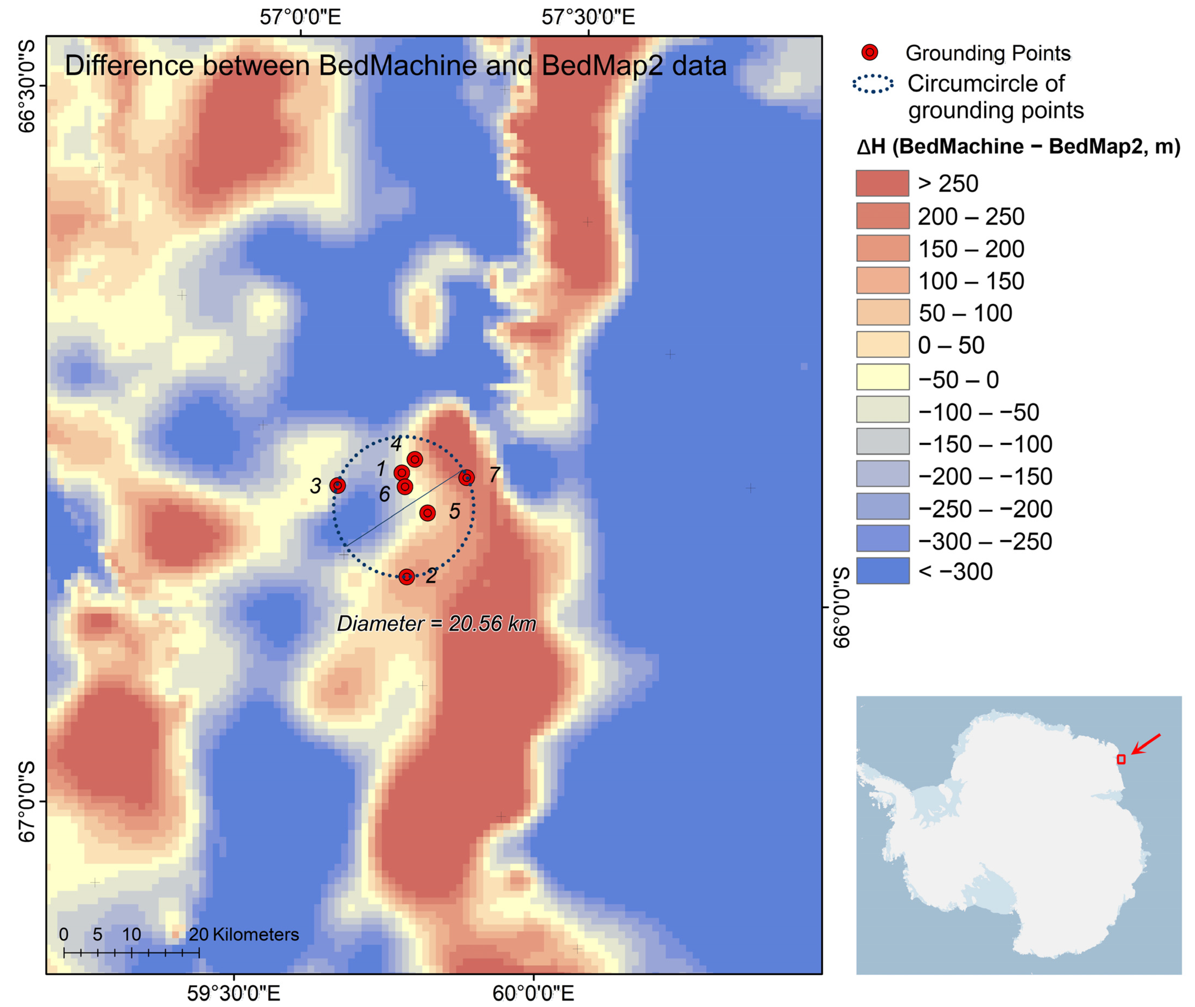
The water depths from seabed elevation models were calculated by subtracting the seabed elevation from mean surface height (). Gaps as large as hundreds of meters were found through the water depths estimated by the grounding event, BedMap2 data, and BedMachine data (Figure 5, Table 3). Only the water depth at grounding point 3 from BedMap2 data established a shallower water than the iceberg draft. The differences implied the slope of the continental shelf off Kemp Coast is not as smooth as it seemed from the seabed maps. The diameter of the circumcircle of the grounding points was 20.56 km, indicating that the inaccuracies of existing seabed elevation data are common phenomena in the study area. There are supposed to be undetected banks or ridges that can impact the mesoscale characteristics of the slope current.
4.3. Wind and Sea Water Velocities of the Study Area
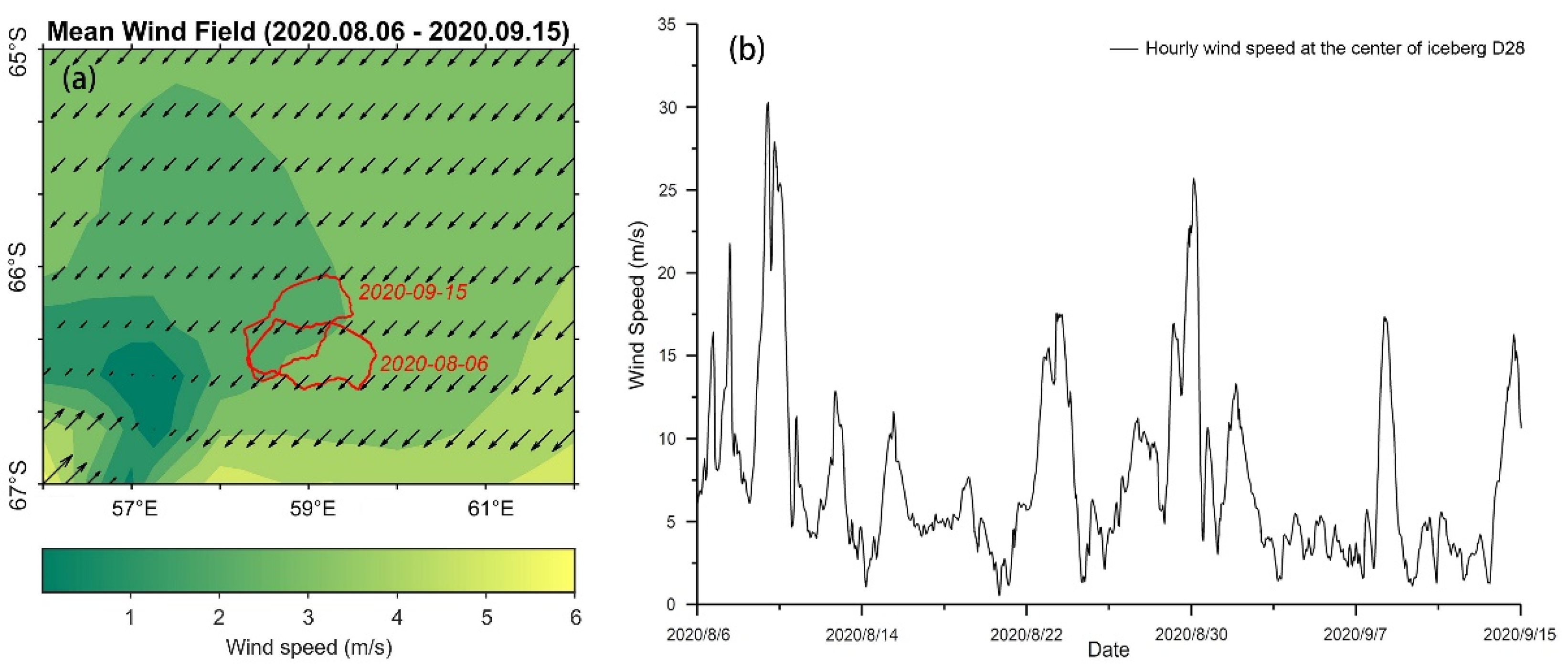
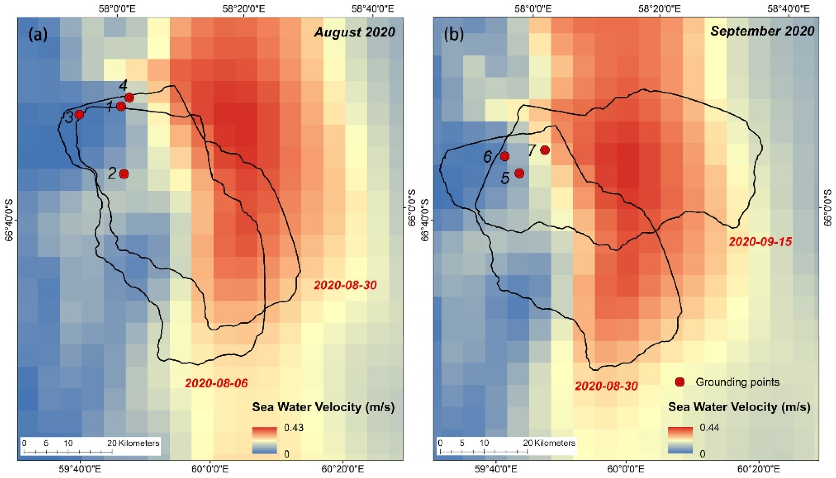
The mean wind velocity of the study area from 6 August to 15 September and its hourly trend is established in Figure 6a,b. The wind blew from the north in the study area, nearly perpendicular to the linear velocity direction of the iceberg. The wind speed peaked on August 9 at over 30 m/s for an instant, while the average speed was about 3 m/s at the iceberg location. The mean sea water speed map is shown in Figure 7a,b, presenting a water speed near to 0 at the grounding points. Meanwhile, its farther end was surrounded by fast running water. With a larger proportion of the iceberg volume proceeding into the area with fast sea water velocity, it moved a longer distance in the first 15 days of September than nearly a whole month of August.
In most situations, the water force is considered to be more dominant than the force by wind for icebergs longer than 12 km [13]. During the study period, the wind field near Kemp Coast illustrated a force with a direction perpendicular to the linear velocity direction of the iceberg. Meanwhile, the sea water velocities did not change much with time during the study period and provided a stable propelling force due to the difference in sea water velocities in the grounding area and the farther end of the iceberg. Thus, we can summarize that the driving force from the sea water was a more important factor than the wind dominating the iceberg motion during the grounding event. This inference is in line with a previous study on iceberg dynamics [13,22,53].
5. Discussion
5.1. Iceberg Draft Estimation
Several assumptions were made in estimating the iceberg draft in this study. First, the iceberg thickness did not change significantly throughout the first year after the calving event. Second, the density model of iceberg D28 was the same as that of its origin on Amery Ice Shelf. Finally, Iceberg D28 was cylindrically shaped with the same areas at its surface and the bottom.
The uncertainty from each assumption is discussed separately.
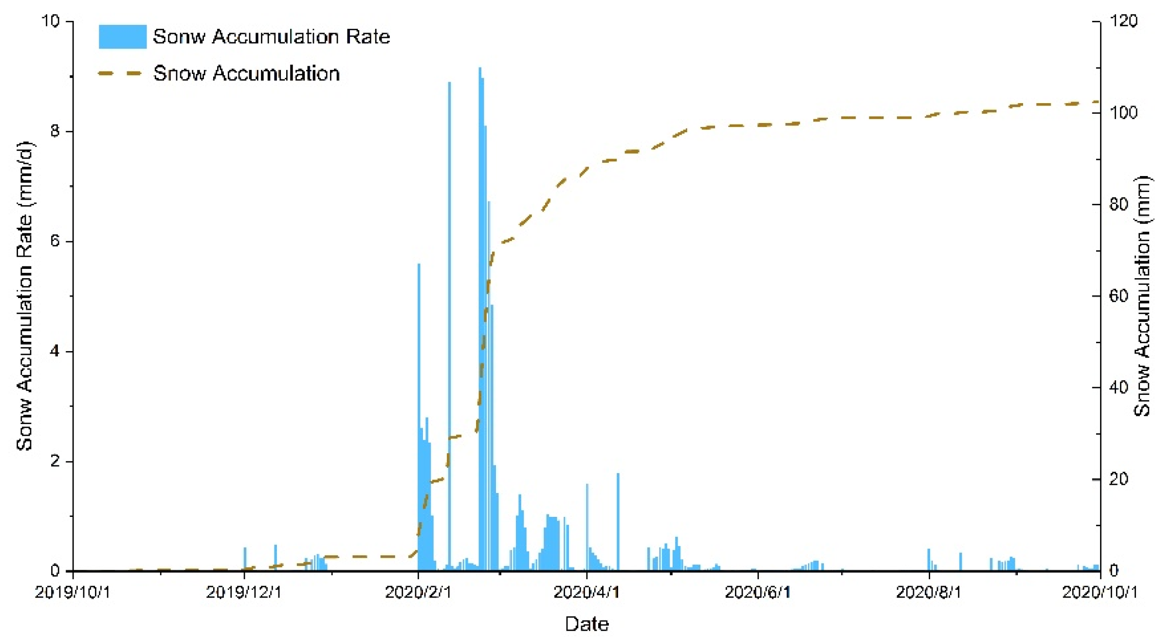
1. According to previous studies on iceberg evolution, processes affecting the iceberg thickness include snow accumulation and basal melting [54]. Snow accumulation can cause an increase in iceberg thickness. Meanwhile, basal melting accounts for 95% of the decrease, and surface melting, together with strain thinning, contributes the other 5% of the thickness change as simulations on large tabular icebergs [55]. Snow accumulation can be estimated with ERA5 reanalysis products by subtracting snowmelt and snow evaporation from snowfall. Hourly snow accumulation was aggregated from October 2019 to September 2020, resulting in 102 mm of snow water equivalent over the iceberg, which equals a snow layer of about 2.87 m thick taking the snow density as 355 kg/m3 (Figure 8). It was insignificant compared to the total thickness of iceberg D28 (Figure 4a), hence the neglect of its impact on thickness change was acceptable.
Influences of basal melting on iceberg thickness have been evaluated by many researchers. The thickness of iceberg A68 decreased by 12.89 ± 3.34 m per year in its first 1.5 years of drifting [22]. The melting rate of iceberg A38B varied from 1.2 m per year to 10.8 m per year with its trajectory from Ronne Ice Shelf to the warm sea water near the Antarctic Peninsula [56]. Iceberg B30 had an average thinning rate of 17.3 ± 1.8 m per year estimated with satellite altimetry data in 6.5 years [23]. Melting rates of icebergs between 60 and 150°E were 11–18 m per year from ship-based observations over 15 years [57]. Though the iceberg melting rate varies dramatically in different regions in the Southern Ocean with water temperature and latitude, we inferred that the thickness of iceberg D28 decreased less than 20 m during the first year after its appearance, since it drifted at a high latitude (Figure 1a). A deviation of 20 m would not change our findings about seabed topography, considering that the maximum water depth estimated through a grounding event has an average disagreement of hundreds of meters with the existing seabed elevation models.
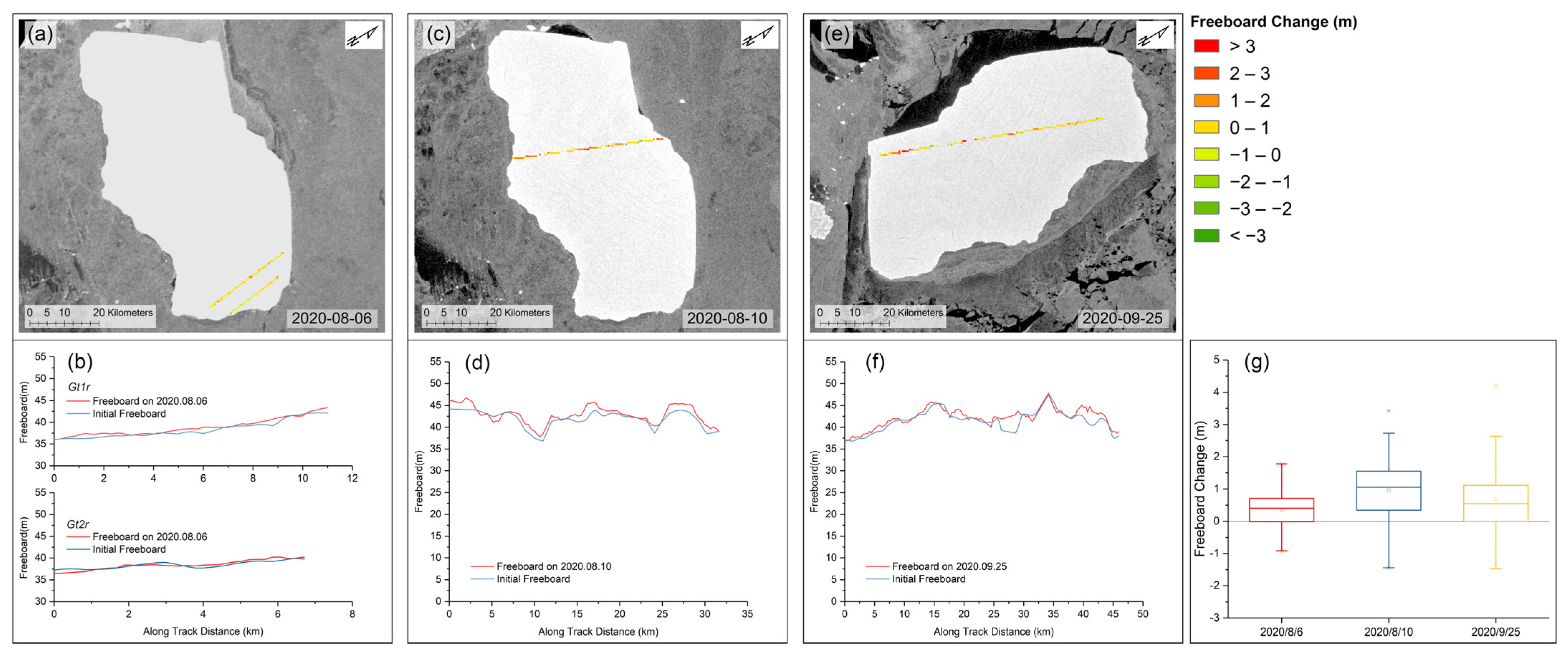
The assumption can be verified with altimeter data. The altimeter ground tracks were mapped onto the iceberg surfaces from near-coincident SAR images (Figure 9a,c,e). We compared the freeboard derived from altimeter ground tracks over the iceberg with its initial surface topography from August 2020 to September 2020 and calculated the differences. The results are shown in Figure 9. The freeboard on 6 August was calculated from ICESat-2 ATL03 product downscaled to 350 m by the algorithm introduced in Algorithm Theoretical Basis Document for ATL06 [58]. Freeboards for 10 August and 25 September were derived from Sentinel-3 SRAL level 2 product. The mean freeboard differences were 0.36 m, 0.96 m, and 0.68 m, respectively. Regardless of the mismatch of surface terrain at some points, the results indicated little freeboard and thickness change within the first year of D28′s drifting.
2. We set the uncertainties of densities of the sea water, snow, and ice to 2 kg/m3, 5.3 kg/m3 (1.5% of 355 kg/m3) [51], and 10 kg/m3, respectively. The freeboard uncertainty was set to 1.59 m, which is the maximum standard deviation in cross validations of different altimeters (Table 1), leaving out the uncertainty in estimating the mean sea surface level. Then, the uncertainty at each grounding point was estimated through Monte Carlo simulations (Table 3). The uncertainty of retrieving the iceberg draft was about 20–25 m on average, suggesting that a field investigation into densities is necessary in order to precisely evaluate iceberg geometric properties.
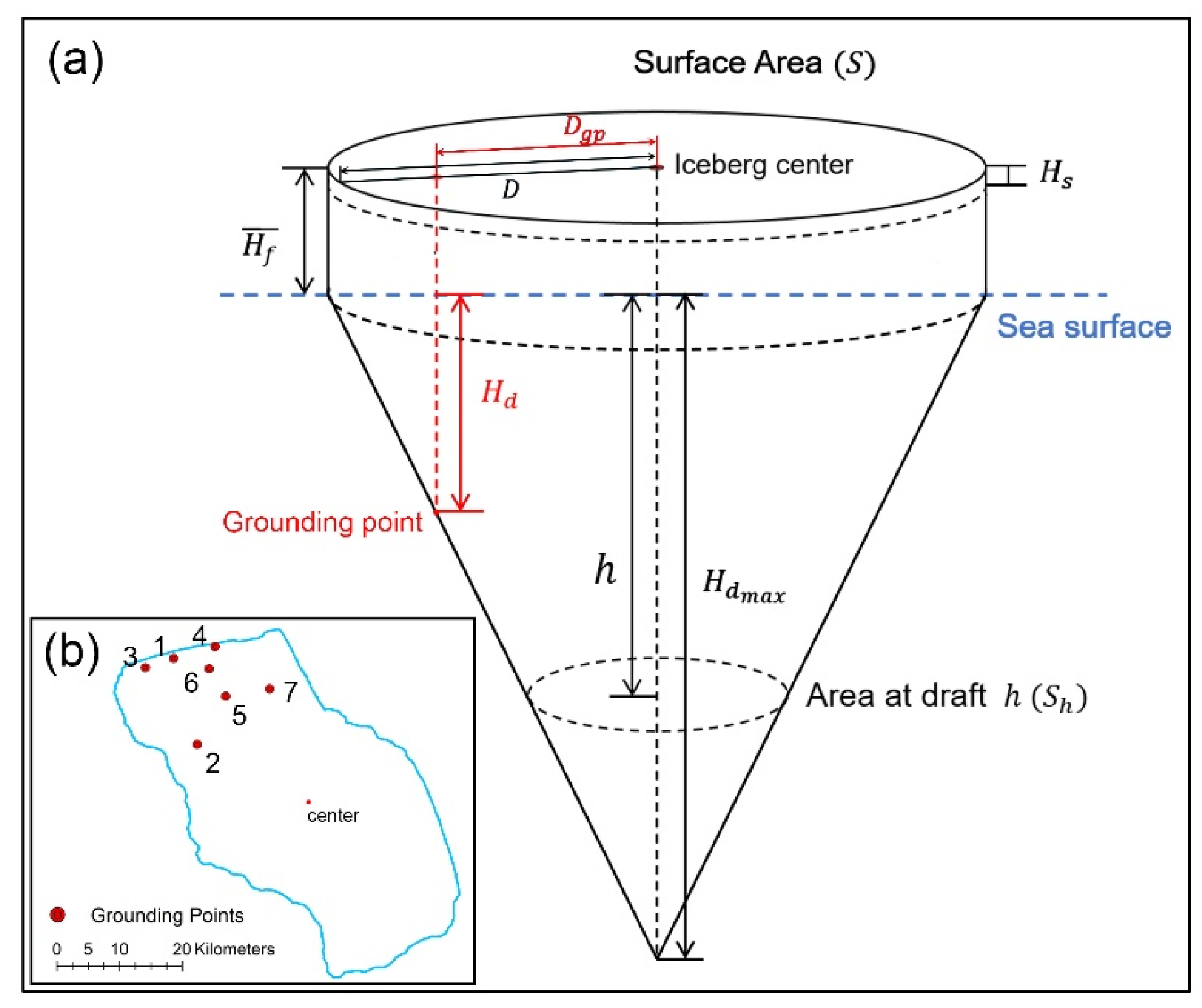
3. The iceberg draft estimation was carried out with a hypothesis that the iceberg had a cylindrical shape under the sea surface, and areas of the surface and the bottom were exactly the same. However, according to bathymetric surveys, the underwater parts of icebergs tend to be irregularly shaped [54]. Here, we considered the ideal case that iceberg D28 maintained a conical shape underwater (Figure 10a). To ensure the center of mass is vertically consistent with the surface center and to simplify the calculation, we used the average freeboard and average ice density to estimate its mass. Thus, according to the buoyancy principle and the relative positions of grounding points to the iceberg center (Figure 10b), the iceberg draft can be calculated with Equation (3):
where is the average freeboard of iceberg D28, which was 40.63 m according to the freeboard map derived from altimetry data; is the surface area; is the cross-sectional area at the draft ; is the maximum iceberg draft; is the average ice density (891 kg/m3); is the horizontal distance from the center to the grounding point; and is the distance from the edge to the center, passing the projection of grounding points on the surface. The maximum iceberg draft () was 746.91 m as a consequence. The iceberg draft at each grounding point is shown in Table 4, and the uncertainties caused by the density model and freeboard estimation were also estimated using Monte Carlo simulations.
Draft at grounding points ranged from 13.40 ± 1.99 m to 326.90 ± 31.58 m through the assumption of iceberg D28 maintaining conical shape under the water line. The results display a tremendous disagreement with the draft of a cylinder-shaped iceberg. Few studies on icebergs consider cone-shaped icebergs. Enderlin et al. explored the melting rate of icebergs in Sermilik Fjord with high-resolution digital elevation models by estimating the submerged area with ideal cylindrical shape and conical shape [59]. The melting rates of both situations were in line with each other, while the drafts differed significantly. Evaluating the iceberg properties requires more specific underwater bathymetric surveys to obtain a knowledge of its immersion topography.
5.2. Seabed Topography Revealed by the Maximum Water Depths at Grounding Points
Although a lack of the underwater geometric parameters of iceberg D28 may lead to a misestimation of its draft, the results in “cylindric-shaped” and “cone-shaped” situations remained consistent with findings about the seabed topography. Water depths estimated by iceberg draft indicated a more complicated topography on the continental land shelf off Kemp Coast than the documented steep slope extending smoothly to the deep ocean (Figure 1b). Most of the results demonstrated a much shallower water area than the existing elevation models, implying the existence of ridges or hills on the continental shelf. Moreover, seabed elevation models from BedMap2 and BedMachine data are not in agreement with each other in this area, presenting elevation gaps from tens to hundreds of meters (Figure 5). The lack of bathymetry data may cause inconsistencies. As a previous study concluded, the area off Kemp Coast is an area where icebergs tend to become grounded [33]. Further studies on grounded icebergs will provide more details about the seabed topography in this area.
6. Conclusions
The main purpose of this study was to estimate the seabed elevation by characterizing the grounded iceberg off Kemp Coast with multiple remote sensing data and to explore the driving force of iceberg motion through reanalysis products during the grounding event. The results indicate that the existence of banks or ridges on the continental shelf near Kemp Coast is not presented by seabed elevation models of BedMap2 and BedMachine data. The terrain features presented by the grounded iceberg extend for at least 20 km in the study area, which can affect the characteristics of the slope current. The force by sea water is a more dominant factor than that of wind in determining the motion of iceberg D28 during the grounding event. The estimation of iceberg draft with different assumptions was also discussed. This research demonstrated the possibility of investigating the seabed topography in the Southern Ocean through grounded icebergs as a supplement to traditional submarine bathymetry. Further studies on grounded icebergs will provide various perspectives on the seabed topography.
Author Contributions
Conceptualization, methodology, formal analysis, investigation, data curation, visualization, and writing—original draft preparation, X.L.; writing—review and editing, X.L., T.L., Q.L., F.P., Z.C. and J.H.; supervision, X.C.; project administration, X.C. All authors have read and agreed to the published version of the manuscript.
Funding
This research was funded by National Natural Science Foundation of China (Grant No. 41925027, 41830536), and Innovation Group Project of Southern Marine Science and Engineering Guangdong Laboratory (Zhuhai) (No. 311021008).
Institutional Review Board Statement
Not applicable.
Informed Consent Statement
Not applicable.
Data Availability Statement
Not applicable.
Acknowledgments
We acknowledge the World Climate Research Programme through its Working Group on Coupled Modelling, who coordinated and promoted CMIP6. We thank the ocean modeling groups for producing and making available their model output, the Earth System Grid Federation (ESGF) for archiving the data and for providing access, and the multiple funding agencies who support CMIP6 and ESGF.
Conflicts of Interest
The author declare no conflict of interest.
References
- Woodworth-Lynas, C.M.T.; Josenhans, H.W.; Barrie, J.V.; Lewis, C.F.M.; Parrott, D.R. The physical processes of seabed disturbance during iceberg grounding and scouring. Cont. Shelf Res. 1991, 11, 939–961. [Google Scholar] [CrossRef]
- MacAyeal, D.R.; Okal, M.H.; Thom, J.E.; Brunt, K.M.; Kim, Y.-J.; Bliss, A.K. Tabular iceberg collisions within the coastal regime. J. Glaciol. 2008, 54, 371–386. [Google Scholar] [CrossRef] [Green Version]
- Bigg, G.R.; Wadley, M.R.; Stevens, D.P.; Johnson, J.A. Modelling the dynamics and thermodynamics of icebergs. Cold Reg. Sci. Technol. 1997, 26, 113–135. [Google Scholar] [CrossRef] [Green Version]
- Clark, J.I.; Landva, J. Geotechnical aspects of seabed pits in the Grand Banks area. Can. Geotech. J. 1988, 25, 448–454. [Google Scholar] [CrossRef]
- McKenna, R.; King, T.; Crocker, G.; Bruneau, S.; German, P. Modelling iceberg grounding on the grand banks. In Proceedings of the International Conference on Port and Ocean Engineering under Arctic Conditions, POAC, Delft, The Netherlands, 9–19 June 2019. [Google Scholar]
- Kuijpers, A.; Dalhoff, F.; Brandt, M.P.; Hümbs, P.; Schott, T.; Zotova, A. Giant iceberg plow marks at more than 1 km water depth offshore West Greenland. Mar. Geol. 2007, 246, 60–64. [Google Scholar] [CrossRef]
- Gebhardt, A.C.; Jokat, W.; Niessen, F.; Matthiessen, J.; Geissler, W.H.; Schenke, H.W. Ice sheet grounding and iceberg plow marks on the northern and central Yermak Plateau revealed by geophysical data. Quat. Sci. Rev. 2011, 30, 1726–1738. [Google Scholar] [CrossRef] [Green Version]
- Normandeau, A.; MacKillop, K.; Macquarrie, M.; Richards, C.; Bourgault, D.; Campbell, D.C.; Maselli, V.; Philibert, G.; Clarke, J.H. Submarine landslides triggered by iceberg collision with the seafloor. Nat. Geosci. 2021, 14, 599–605. [Google Scholar] [CrossRef]
- Barnes, D.K.A.; Fleming, A.; Sands, C.J.; Quartino, M.L.; Deregibus, D. Icebergs, sea ice, blue carbon and Antarctic climate feedbacks. Philos. Trans. R. Soc. A Math. Phys. Eng. Sci. 2018, 376, 20170176. [Google Scholar] [CrossRef] [Green Version]
- Gutt, J. On the direct impact of ice on marine benthic communities, a review. Polar Biol. 2001, 24, 553–564. [Google Scholar] [CrossRef]
- Teixido, N.; Garrabou, J.; Gutt, J.; Arntz, W.E. Iceberg disturbance and successional spatial patterns: The case of the shelf Antarctic benthic communities. Ecosystems 2007, 10, 142–157. [Google Scholar] [CrossRef]
- Barnes, D.K.A.; Souster, T. Reduced survival of Antarctic benthos linked to climate-induced iceberg scouring. Nat. Clim. Chang. 2011, 1, 365–368. [Google Scholar] [CrossRef]
- Wagner, T.J.W.; Dell, R.W.; Eisenman, I.; Dell, R.W.; Wagner, T.J.W.; Dell, R.W.; Eisenman, I. An Analytical Model of Iceberg Drift. J. Phys. Oceanogr. 2017, 47, 1605–1616. [Google Scholar] [CrossRef]
- Tournadre, J.; Bouhier, N.; Girard-Ardhuin, F.; Remy, F. Large icebergs characteristics from altimeter waveforms analysis. J. Geophys. Res. 2015, 120, 1954–1974. [Google Scholar] [CrossRef]
- Liu, Y.; Cheng, X.; Hui, F.; Wang, F.; Chi, Z. Antarctic iceberg calving monitoring based on EnviSat ASAR images. Yaogan Xuebao J. Remote Sens. 2013, 17, 479–494. [Google Scholar]
- Ballantyne, J.; Long, D.G. A multidecadal study of the number of antarctic icebergs using scatterometer data. In Proceedings of the IEEE International Geoscience and Remote Sensing Symposium, Toronto, ON, Canada, 24–28 June 2002; pp. 3029–3031. [Google Scholar]
- Budge, J.; Long, D. Estimating Sizes and Rotation Angles of Antarctic Icebergs Utilizing Scatterometer Data. In Proceedings of the 2017 IEEE International Geoscience and Remote Sensing Symposium, Fort Worth, TX, USA, 4 December 2017; pp. 3585–3588. [Google Scholar]
- Luckman, A.; Padman, L.; Jansen, D. Persistent iceberg groundings in the western Weddell Sea, Antarctica. Remote Sens. Environ. 2010, 114, 385–391. [Google Scholar] [CrossRef]
- Li, T.T.; Shokr, M.; Liu, Y.; Cheng, X.; Li, T.T.; Wang, F.; Hui, F. Monitoring the tabular icebergs C28A and C28B calved from the Mertz Ice Tongue using radar remote sensing data. Remote Sens. Environ. 2018, 216, 615–625. [Google Scholar] [CrossRef]
- Abe, T.; Ohki, M.; Tadono, T. Observation of Huge Iceberg Detachment from Larsen-C Ice Shelf in Antarctic Peninsula by Alos-2/Palsar-2. In Proceedings of the IGARSS 2018—2018 IEEE International Geoscience and Remote Sensing Symposium, Valencia, Spain, 5 November 2018; pp. 5172–5175. [Google Scholar]
- Hawkins, J.D.; Laxon, S.; Phillips, H. Antarctic Tabular Iceberg MultiSensor Mapping. In Proceedings of the IGARSS’91 Remote Sensing: Global Monitoring for Earth Management, Espoo, Finland, 3–6 June 1991. [Google Scholar]
- Han, H.; Lee, S.; Kim, J.I.; Kim, S.H.; Kim, H.C. Changes in a Giant Iceberg Created from the Collapse of the Larsen C Ice Shelf, Antarctic Peninsula, Derived from Sentinel-1 and CryoSat-2 Data. Remote Sens. 2019, 11, 404. [Google Scholar] [CrossRef] [Green Version]
- Braakmann-Folgmann, A.; Shepherd, A.; Ridout, A. Tracking changes in the area, thickness, and volume of the Thwaites tabular iceberg “B30” using satellite altimetry and imagery. Cryosphere 2021, 15, 3861–3876. [Google Scholar] [CrossRef]
- Jacobs, S.S. On the nature and significance of the Antarctic Slope Front. Mar. Chem. 1991, 35, 9–24. [Google Scholar] [CrossRef]
- Nakayama, Y.; Ohshima, K.I.; Matsumura, Y.; Fukamachi, Y.; Hasumi, H. A numerical investigation of formation and variability of Antarctic bottom water off Cape Darnley, East Antarctica. J. Phys. Oceanogr. 2014, 44, 2921–2937. [Google Scholar] [CrossRef]
- Thompson, A.F.; Stewart, A.L.; Spence, P.; Heywood, K.J. The Antarctic Slope Current in a Changing Climate. Rev. Geophys. 2018, 56, 741–770. [Google Scholar] [CrossRef]
- Stewart, A.L.; Klocker, A.; Menemenlis, D. Circum-Antarctic Shoreward Heat Transport Derived From an Eddy- and Tide-Resolving Simulation. Geophys. Res. Lett. 2018, 45, 834–845. [Google Scholar] [CrossRef] [Green Version]
- Delpeche-Ellmann, N.; Soomere, T.; Kudryavtseva, N. The role of nearshore slope on cross-shore surface transport during a coastal upwelling event in Gulf of Finland, Baltic Sea. Estuar. Coast. Shelf Sci. 2018, 209, 123–135. [Google Scholar] [CrossRef]
- St-Laurent, P.; Klinck, J.M.; Dinniman, M.S. On the role of coastal troughs in the circulation of warm circumpolar deep water on Antarctic shelves. J. Phys. Oceanogr. 2013, 43, 51–64. [Google Scholar] [CrossRef] [Green Version]
- Ott, N.; Schenke, H.W. International Bathymetric Chart of the Southern Ocean (IBCSO). In Proceedings of the SCAR/IASC/IPY Open Science Conference, St. Petersburg, Russia, 8–11 July 2008. [Google Scholar]
- Schaffer, J.; Timmermann, R.; Erik Arndt, J.; Savstrup Kristensen, S.; Mayer, C.; Morlighem, M.; Steinhage, D. A global, high-resolution data set of ice sheet topography, cavity geometry, and ocean bathymetry. Earth Syst. Sci. Data 2016, 8, 543–557. [Google Scholar] [CrossRef] [Green Version]
- Fretwell, P.; Pritchard, H.D.; Vaughan, D.G.; Bamber, J.L.; Barrand, N.E.; Bell, R.; Bianchi, C.; Bingham, R.G.; Blankenship, D.D.; Casassa, G.; et al. Bedmap2: Improved ice bed, surface and thickness datasets for Antarctica. Cryosphere 2013, 7, 375–393. [Google Scholar] [CrossRef] [Green Version]
- Li, T.; Liu, Y.; Cheng, X.; Ouyang, L.X.; Li, X.Q.; Liu, J.P.; Shokr, M.; Hui, F.M.; Zhang, J.; Wen, J. The effect of seafloor topography in the Southern Ocean on tabular iceberg drifting and grounding. Sci. China Earth Sci. 2017, 60, 697–706. [Google Scholar] [CrossRef]
- Torres, R.; Snoeij, P.; Geudtner, D.; Bibby, D.; Davidson, M.; Attema, E.; Potin, P.; Rommen, B.Ö.; Floury, N.; Brown, M.; et al. GMES Sentinel-1 mission. Remote Sens. Environ. 2012, 120, 9–24. [Google Scholar] [CrossRef]
- Justice, C.O.; Townshend, J.R.G.; Vermote, E.F.; Masuoka, E.; Wolfe, R.E.; Saleous, N.; Roy, D.P.; Morisette, J.T. An overview of MODIS Land data processing and product status. Remote Sens. Environ. 2002, 83, 3–15. [Google Scholar] [CrossRef]
- Mcmillan, M.; Shepherd, A.; Sundal, A.; Briggs, K.; Muir, A.; Ridout, A.; Hogg, A.; Wingham, D. Increased ice losses from Antarctica detected by CryoSat-2. Geophys. Res. Lett. 2014, 41, 3899–3905. [Google Scholar] [CrossRef]
- Meloni, M.; Bouffard, J.; Parrinello, T.; Dawson, G.; Garnier, F.; Helm, V.; Di Bella, A.; Hendricks, S.; Ricker, R.; Webb, E.; et al. CryoSat Ice Baseline-D validation and evolutions. Cryosphere 2020, 14, 1889–1907. [Google Scholar] [CrossRef]
- Quartly, G.D.; Nencioli, F.; Raynal, M.; Bonnefond, P.; Garcia, P.N.; Garcia-Mondéjar, A.; de la Cruz, A.F.; Cretaux, J.F.; Taburet, N.; Frery, M.L.; et al. The roles of the S3MPC: Monitoring, validation and evolution of sentinel-3 altimetry observations. Remote Sens. 2020, 12, 1763. [Google Scholar] [CrossRef]
- Parrish, C.E.; Magruder, L.A.; Neuenschwander, A.L.; Forfinski-Sarkozi, N.; Alonzo, M.; Jasinski, M. Validation of ICESat-2 ATLAS bathymetry and analysis of ATLAS’s bathymetric mapping performance. Remote Sens. 2019, 12, 1763. [Google Scholar] [CrossRef] [Green Version]
- Dowdeswell, J.A.; Bamber, J.L. Keel depths of modern Antarctic icebergs and implications for sea-floor scouring in the geological record. Mar. Geol. 2007, 243, 120–131. [Google Scholar] [CrossRef]
- Hersbach, H.; Bell, B.; Berrisford, P.; Hirahara, S.; Horányi, A.; Muñoz-Sabater, J.; Nicolas, J.; Peubey, C.; Radu, R.; Schepers, D.; et al. The ERA5 global reanalysis. Q. J. R. Meteorol. Soc. 2020, 146, 1999–2049. [Google Scholar] [CrossRef]
- Roberts, M. MOHC HadGEM3-GC31-HH Model Output Prepared for CMIP6 HighResMIP Highres-Future, Version 20200731. Earth System Grid Federation. 2019. Available online: https://cera-www.dkrz.de/WDCC/ui/cerasearch/cmip6?input=CMIP6.HighResMIP.MOHC.HadGEM3-GC31-HH.highres-future (accessed on 23 December 2021). [CrossRef]
- Morlighem, M.; Rignot, E.; Binder, T.; Blankenship, D.; Drews, R.; Eagles, G.; Eisen, O.; Ferraccioli, F.; Forsberg, R.; Fretwell, P.; et al. Deep glacial troughs and stabilizing ridges unveiled beneath the margins of the Antarctic ice sheet. Nat. Geosci. 2020, 13, 132–137. [Google Scholar] [CrossRef]
- Padman, L.; Fricker, H.A.; Coleman, R.; Howard, S.; Erofeeva, L. A new tide model for the Antarctic ice shelves and seas. Ann. Glaciol. 2002, 34, 247–254. [Google Scholar] [CrossRef] [Green Version]
- Rignot, E.; Mouginot, J.; Scheuchl, B. Ice Flow of the Antarctic Ice Sheet. Science 2011, 333, 1427–1430. [Google Scholar] [CrossRef] [Green Version]
- Mouginot, J.; Scheuchl, B.; Rignot, E.; Scheuch, B.; Rignot, E. Mapping of Ice Motion in Antarctica Using Synthetic-Aperture Radar Data. Remote Sens. 2012, 4, 2753–2767. [Google Scholar] [CrossRef] [Green Version]
- Förste, C.; Bruinsma, S.; Abrikosov, O.; Flechtner, F.; Marty, J.-C.; Lemoine, J.-M.; Dahle, C.; Neumayer, H.; Barthelmes, F.; König, R.; et al. EIGEN-6C4—The latest combined global gravity field model including GOCE data up to degree and order 1949 of GFZ Potsdam and GRGS Toulouse. In Proceedings of the EGU General Assembly Conference, Vienna, Austria, 27 April–2 May 2014; p. 3707. [Google Scholar]
- Knudsen, P.; Andersen, O.B.; Maximenko, N. The updated geodetic mean dynamic topography model—DTU15MDT. In Proceedings of the EGU General Assembly Conference, Vienna, Austria, 17–22 April 2016. [Google Scholar]
- Chuter, S.J.; Bamber, J.L. Antarctic ice shelf thickness from CryoSat-2 radar altimetry. Geophys. Res. Lett. 2015, 42, 10721–10729. [Google Scholar] [CrossRef] [Green Version]
- Wen, J.; Jezek, K.C.; Csathó, B.M.; Herzfeld, U.C.; Farness, K.L.; Huybrechts, P. Mass budgets of the Lambert, Mellor and Fisher Glaciers and basal fluxes beneath their flowbands on Amery Ice Shelf. Sci. China Ser. D Earth Sci. 2007, 50, 1693–1706. [Google Scholar] [CrossRef] [Green Version]
- Weinhart, A.H.; Freitag, J.; Hörhold, M.; Kipfstuhl, S.; Eisen, O. Representative surface snow density on the East Antarctic Plateau. Cryosphere 2020, 14, 3663–3685. [Google Scholar] [CrossRef]
- Craven, M.; Allison, I.; Fricker, H.A.; Warner, R. Properties of a marine ice layer under the Amery Ice Shelf, East Antarctica. J. Glaciol. 2009, 55, 717–728. [Google Scholar] [CrossRef] [Green Version]
- Romanov, Y.A.; Romanova, N.A.; Romanov, P. Shape and size of Antarctic icebergs derived from ship observation data. Antarct. Sci. 2011, 24, 77–87. [Google Scholar] [CrossRef]
- Bigg, G.R. Icebergs: Their Science and Links to Global Change; Cambridge University Press (CUP): Cambridge, UK, 2015; ISBN 9781107067097. [Google Scholar]
- Jansen, D.; Sandhäger, H.; Rack, W. Model experiments on large tabular iceberg evolution: Ablation and strain thinning. J. Glaciol. 2005, 51, 363–372. [Google Scholar] [CrossRef] [Green Version]
- Jansen, D.; Schodlok, M.; Rack, W. Basal melting of A-38B: A physical model constrained by satellite observations. Remote Sens. Environ. 2007, 111, 195–203. [Google Scholar] [CrossRef]
- Jacka, T.H.; Giles, A.B. Antarctic iceberg distribution and dissolution from ship-based observations. J. Glaciol. 2007, 53, 341–356. [Google Scholar] [CrossRef] [Green Version]
- Smith, B.; Hancock, D.; Harbeck, K.; Roberts, L.; Neumann, T.; Brunt, K.; Fricker, H.; Gardner, A.; Siegfried, M.; Adusumilli, S. Algorithm Theoretical Basis Document (ATBD) for Land Ice Along-Track Height Product (ATL06). In ICE, CLOUD, and Land Elevation Satellite-2 (ICESat-2) Project; Goddard Space Flight Center: Greenbelt, MA, USA, 2019. [Google Scholar]
- Enderlin, E.M.; Hamilton, G.S. Estimates of iceberg submarine melting from high-resolution digital elevation models: Application to Sermilik Fjord, East Greenland. J. Glaciol. 2017, 60, 1084–1092. [Google Scholar] [CrossRef] [Green Version]
Figure 1.
Drifting and grounding of iceberg D28. (a) Trajectory from September 2019 to February 2021. (b) Motion of the iceberg in the grounding area with contour map of seabed elevation from Bedmap2. The iceberg boundaries are delineated from Sentinel-1 SAR images obtained on (c) 6 August, (d) 30 August, (e) 15 September, and (f) 25 September.

Figure 2.
Altimetry data used to estimate the draft of iceberg D28. (a) Cryosat-2, (b) Sentinel-3, and (c) ICESat-2 data distributions over the front part of Amery Ice Shelf with a base image from Sentinel-1 on 20 September 2019.
Figure 2.
Altimetry data used to estimate the draft of iceberg D28. (a) Cryosat-2, (b) Sentinel-3, and (c) ICESat-2 data distributions over the front part of Amery Ice Shelf with a base image from Sentinel-1 on 20 September 2019.

Figure 3.
Diagram for calculating the speed of different parts of the iceberg.

Figure 4.
(a) Thickness map and (b) draft map of iceberg D28. (c) A Sentinel-1 SAR image obtained on 28 December 2019. The topographic relieves shown by the thickness map and the satellite image are marked by the red ellipses.
Figure 4.
(a) Thickness map and (b) draft map of iceberg D28. (c) A Sentinel-1 SAR image obtained on 28 December 2019. The topographic relieves shown by the thickness map and the satellite image are marked by the red ellipses.

Figure 5.
Locations and the circumcircle of grounding points and the difference between seabed elevations from BedMachine and BedMap2 data.
Figure 5.
Locations and the circumcircle of grounding points and the difference between seabed elevations from BedMachine and BedMap2 data.

Figure 6.
Wind field over the grounding area. (a) Mean wind velocity and (b) hourly wind speed trend at the center of iceberg D28 from 6 August to 15 September.
Figure 6.
Wind field over the grounding area. (a) Mean wind velocity and (b) hourly wind speed trend at the center of iceberg D28 from 6 August to 15 September.

Figure 7.
Mean sea water speed around iceberg D28 and the grounding points in (a) August 2020 and (b) September 2020.
Figure 7.
Mean sea water speed around iceberg D28 and the grounding points in (a) August 2020 and (b) September 2020.

Figure 8.
The snow accumulation rate and total snow accumulation curve over iceberg D28 from October 2019 to October 2020.
Figure 8.
The snow accumulation rate and total snow accumulation curve over iceberg D28 from October 2019 to October 2020.

Figure 9.
The altimeter ground tracks mapped on the iceberg surface on 6 August (a), 10 August (c), and 25 September (e) of 2020, and the corresponding freeboard differences along the tracks (b),(d), and (f), respectively. (g) The box plot of freeboard differences.
Figure 9.
The altimeter ground tracks mapped on the iceberg surface on 6 August (a), 10 August (c), and 25 September (e) of 2020, and the corresponding freeboard differences along the tracks (b),(d), and (f), respectively. (g) The box plot of freeboard differences.

Figure 10.
Illustration of an ideal cone-shaped iceberg. (a) Iceberg sketch and variables used. (b) Grounding points mapped onto the iceberg surface delineated from satellite image on 30 August 2020.
Figure 10.
Illustration of an ideal cone-shaped iceberg. (a) Iceberg sketch and variables used. (b) Grounding points mapped onto the iceberg surface delineated from satellite image on 30 August 2020.


Table 1.
Cross validation of the three altimeters on Cryosat-2, Sentinel-3, and ICESat-2 over Amery Front before the calving event.
Table 1.
Cross validation of the three altimeters on Cryosat-2, Sentinel-3, and ICESat-2 over Amery Front before the calving event.
| Number of Points | Std (m) | ||
|---|---|---|---|
| ICESat-2–Cryosat-2 | 5663 | 0.78 | 0.81 |
| ICESat-2–Sentinel-3 | 6182 | 0.49 | 1.15 |
| Sentinel-3–Cryosat-2 | 239 | −0.21 | 1.59 |
Table 2.
The iceberg’s moving speed range every four days from 6 August to 15 September 2020.
| Date | Min Speed (m/day) | Max Speed (m/day) | No. of Grounding Point |
|---|---|---|---|
| 6 August–10 August | 365.7 ± 20 | 721.5 ± 20 | − |
| 10 August–14 August | 21.5 ± 72.5 | 2482.5 ± 72.5 | 1 |
| 14 August–18 August | 17.9 ± 72.5 | 1692.5 ± 72.5 | 2 |
| 18 August–22 August | 306.2 ± 20 | 400.2 ± 20 | − |
| 22 August–26 August | 252.4 ± 72.5 | 613.7 ± 72.5 | − |
| 26 August–30 August | 2.8 ± 72.5 | 1136.7 ± 72.5 | 3 |
| 30 August–3 September | 3.2 ± 20 | 577.5 ± 20 | 4 |
| 3 September–7 September | 8.1 ± 72.5 | 2281.4 ± 72.5 | 5 |
| 7 September–11 September | 40.7 ± 72.5 | 3982.8 ± 72.5 | 6 |
| 11 September–15 September | 18.4 ± 20 | 1996.0 ± 20 | 7 |
Table 3.
Maximum water depths () at grounding points and the corresponding seabed elevations from BedMap2 and BedMachine (), together with the differences in water depths estimated .
Table 3.
Maximum water depths () at grounding points and the corresponding seabed elevations from BedMap2 and BedMachine (), together with the differences in water depths estimated .
| No. | (m) | ||||
|---|---|---|---|---|---|
| 1 | 227.35 ± 22.10 | −356 | 149.09 | −451.55 | 244.64 |
| 2 | 269.42 ± 25.66 | −776 | 527.02 | −626.65 | 377.67 |
| 3 | 221.72 ± 21.77 | −158 | −43.28 | −280.27 | 78.99 |
| 4 | 229.77 ± 22.50 | −463 | 253.67 | −436.28 | 226.95 |
| 5 | 263.48 ± 25.15 | −505 | 261.96 | −517.49 | 274.45 |
| 6 | 250.82 ± 24.23 | −385 | 154.62 | −460.57 | 230.19 |
| 7 | 251.20 ± 24.21 | −831 | 600.24 | −542.14 | 311.38 |
Table 4.
Iceberg draft () at grounding points with the assumption of a conical shape below sea surface, which was also the maximum water depth (), and the corresponding seabed elevation BedMap2 () and BedMachine ().
Table 4.
Iceberg draft () at grounding points with the assumption of a conical shape below sea surface, which was also the maximum water depth (), and the corresponding seabed elevation BedMap2 () and BedMachine ().
| No. | |||||
|---|---|---|---|---|---|
| 1 | 32.01 ± 3.38 | −356 | 344.43 | −451.55 | 439.98 |
| 2 | 326.90 ± 31.58 | −776 | 469.54 | −626.65 | 320.18 |
| 3 | 40.17 ± 4.08 | −158 | 138.27 | −280.27 | 260.54 |
| 4 | 13.40 ± 1.99 | −463 | 470.04 | −436.28 | 443.3 |
| 5 | 244.32 ± 23.62 | −505 | 281.12 | −517.49 | 293.62 |
| 6 | 109.96 ± 10.72 | −385 | 295.48 | −460.57 | 371.05 |
| 7 | 240.82 ± 23.29 | −831 | 610.62 | −542.14 | 321.7 |
Publisher’s Note: MDPI stays neutral with regard to jurisdictional claims in published maps and institutional affiliations. |
© 2021 by the authors. Licensee MDPI, Basel, Switzerland. This article is an open access article distributed under the terms and conditions of the Creative Commons Attribution (CC BY) license (https://creativecommons.org/licenses/by/4.0/).
Share and Cite
MDPI and ACS Style
Liu, X.; Cheng, X.; Liang, Q.; Li, T.; Peng, F.; Chi, Z.; He, J. Grounding Event of Iceberg D28 and Its Interactions with Seabed Topography. Remote Sens. 2022, 14, 154. https://0-doi-org.brum.beds.ac.uk/10.3390/rs14010154
AMA Style
Liu X, Cheng X, Liang Q, Li T, Peng F, Chi Z, He J. Grounding Event of Iceberg D28 and Its Interactions with Seabed Topography. Remote Sensing. 2022; 14(1):154. https://0-doi-org.brum.beds.ac.uk/10.3390/rs14010154
Chicago/Turabian StyleLiu, Xuying, Xiao Cheng, Qi Liang, Teng Li, Fukai Peng, Zhaohui Chi, and Jiaying He. 2022. "Grounding Event of Iceberg D28 and Its Interactions with Seabed Topography" Remote Sensing 14, no. 1: 154. https://0-doi-org.brum.beds.ac.uk/10.3390/rs14010154
Note that from the first issue of 2016, this journal uses article numbers instead of page numbers. See further details here.