
A Bidirectional Deep-Learning-Based Spectral Attention Mechanism for Hyperspectral Data Classification


1
Computer and Information Sciences, The University of Alabama in Huntsville, Huntsville, AL 35899, USA
2
Computer Science and the Big Data Analytics Lab, The University of Alabama in Huntsville, Huntsville, AL 35899, USA
*
Author to whom correspondence should be addressed.
†
These authors contributed equally to this work.
Remote Sens. 2022, 14(1), 217; https://0-doi-org.brum.beds.ac.uk/10.3390/rs14010217
Submission received: 29 November 2021
/
Revised: 29 December 2021
/
Accepted: 31 December 2021
/
Published: 4 January 2022
(This article belongs to the Special Issue New Insights into Hyperspectral Image Processing Methods in Remote Sensing)
Abstract
:Hyperspectral remote sensing presents a unique big data research paradigm through its rich information captured across hundreds of spectral bands, which embodies vital spatial and temporal information about the underlying land cover. Deep-learning-based hyperspectral data analysis methodologies have made significant advancements over the past few years. Despite their success, most deep learning frameworks for hyperspectral data classification tend to suffer in terms of computational and classification efficacy as the data size increases. This is largely due to their equal emphasis criteria on the rich spectral information present in the data, albeit all of the spectral information not being essential for hyperspectral data analysis. On the contrary, this redundant information present in the spectral bands can deter the performance of hyperspectral data analysis techniques. Therefore, in this work, we propose a novel bidirectional spectral attention mechanism, which is computationally efficient and capable of adaptive spectral information diversification through selective emphasis on spectral bands that comprise more information and suppress the ones with lesser information. The concept of 3D-convolutions in tandem with bidirectional long short-term memory (LSTM) is used in the proposed architecture as spectral attention mechanism. A feedforward neural network (FNN)-based supervised classification is then performed to validate the performance of our proposed approach. Experimental results reveal that the proposed hyperspectral data analysis model with spectral attention mechanism outperforms other spatial- and spectral-information-extraction-based hyperspectral data analysis techniques compared.
1. Introduction
The increase in data volume, velocity, and diversity has lately given rise to the term “Big Data”, which symbolizes the multifaceted issues faced by many of the scientific and applied domains. In the context of remote sensing the current data acquisition sources for Earth observation generate vast amounts of data, which are typically images acquired at various scales (high/low) and resolutions (i.e., spatial, spectral/temporal) [1]. Over the past decade, machine learning and deep learning methodologies have gained wide recognition for hyperspectral data analysis in remote sensing applications [2,3]. Deep-learning-based feature extraction and classification methodologies in hyperspectral remote sensing applications using convolutional neural networks (CNNs) [4], recurrent neural networks (RNNs) [5], and their variations foster the automation of processes due to their potential for progressively learning the attributes and information present in the high-dimensional hyperspectral data [6]. Needless to say, the more complex deep-learning-based classification/object detection frameworks are, the higher their subsequent computational overhead is expected to be. However, this high computational cost is not desirable as we gravitate towards more automated/real-time hyperspectral data analysis applications [7].
The Earth’s land cover is a dynamic canvas on which human beings and natural systems are always interacting. Land use/land cover (LULC) classification and its dynamics, which partially result from land surface processes, have considerable effects on biotic diversity, soil degradation, terrestrial ecosystems, and the ability of biological systems to support human needs [8]. Thus, land cover classification, and its dynamics with remote sensing data, is an important field in environmental change research at different scales. The efficient assessment and monitoring of land cover changes are indispensable to advance our understanding of the mechanisms of change and model the effects of these changes on the environment and associated ecosystems at different scales [9].
Remote sensing techniques represent some of the most effective tools to obtain information on LULC classification and dynamics (i.e., temporal–spatial changes and the transformation of landscapes). Many methods can detect land cover changes based on optical and radar imagery with different spatial and spectral resolutions. Existing techniques for accomplishing land cover classification can be broadly grouped into three general types, namely supervised classification algorithms, unsupervised classification algorithms, and a mixture of supervised and unsupervised classification techniques [8]. A large amount of high-dimensional, high-spatial–spectral resolution hyperspectral remote sensing data is becoming available due to the fast development of satellite and sensor technology, and the above-mentioned supervised and unsupervised classification methods could swiftly obtain cardinal information from the remote sensing data, thus playing an important role in hyperspectral imagery applications [10]. This being said, over time, classification frameworks based on high spatial–spectral resolution hyperspectral remote sensing data using machine learning algorithms such as neural networks have made a great impact in the field of remote sensing and our work is directly related to this.
Conventional machine-learning-based hyperspectral imagery classification and object detection frameworks are heavily inclined towards operating on spectral information as features [11]. Most of the spectral-information-reliant frameworks suggested in the literature include some form of similarity- or dissimilarity-distance-measure-based band grouping [12], and traditional supervised classification paradigms using k-nearest neighbors [13], maximum likelihood criterion [14], logistic regression [15], random forest classification [16], bagging and boosting techniques like AdaBoost [17], etc., have proved to be effective in classifying HSI data. Most of these spectral-information-based methodologies lack the potential to capture and utilize the corresponding spectral variability and information effectively, that is readily available in the high-dimensional hyperspectral data. This problem of information extraction and processing such high-dimensional data is not contemporary, however, it has started to gain more importance lately due to the surge in the volume of data (big data) and its acquisition methodologies. The big data attributes directly imply high dimensionality and data redundancy, which in turn exacerbates the curse of dimensionality caveat [18].
As a consequence, dimensionality reduction (DR) plays a prominent role in hyperspectral data analysis [19]. In general, DR techniques help combat the intensive data learning overhead by projecting high-dimensional data from their original feature space to a lower dimensional subspace and preserving all the vital information present in the data. Additionally, DR also brings down the computational requirements by a considerable factor. In the literature, various DR techniques such as principal component analysis (PCA) [20], linear discriminant analysis (LDA) [21], random projections (RPs) [4,6,22], etc., have gained increased attention due to their demonstrated computational efficacy and ability to preserve vital information present in the hyperspectral data. In addition, recent literature has proven that the integration of any form of additional information, such as spatial or contextual, alongside an efficient DR technique, to the available spectral information can improve the efficacy of hyperspectral data analysis [23,24].
In hyperspectral imaging, the relationship between the acquired spectral information and underlying land cover material is inherently nonlinear. To combat this issue, deep learning and machine learning algorithms have generally been adopted as fundamental feature extraction tools for effectively addressing/modeling data with nonlinear intrinsic relationships in the past few years. As a result, such deep learning techniques have shown promising results in the realm of hyperspectral data learning and representation for classification [2], object recognition [25], and other remote sensing applications. However, one of the major shortcomings of these techniques is how the data are presented to the deep learning framework for generalization. Generally, the information extracted from each spectral band is assigned an equal emphasis or importance without any consideration to the significance of spectral information/features on the final data analysis outcome [26,27]. Moreover, this form of antiquated equal importance designation to all the spectral bands can lead to the inclusion of inherent noise or redundant spectral information, which can not only be detrimental to hyperspectral data analysis but also affect the generalization capability of the underlying deep-learning-based HSI analysis framework. Thereby, it can severely inhibit the automation capabilities and efficacy of the methodology [7,23,28].
Therefore, this work leverages the benefits of DR techniques in conjunction with the ability of spatial–spectral representation provided by deep learning techniques to formulate an adaptive spectral attention framework for hyperspectral data analysis. In this framework, the input high-dimensional hyperspectral cube is first reduced to its lower dimensional subspace using principal component analysis (PCA). PCA is an unsupervised linear feature extraction method that uses orthogonal transformation to explore the correlation between the HSI spectral bands in order to extract their intrinsic properties. It is based on the notion that contiguous bands of HSI data are highly correlated and typically convey the same information about the ground objects in order to function efficiently [29]. Following the PCA-based DR, this reduced dimensional data are input to the proposed 3D-convolution [30] and bidirectional LSTM [31] based spectral attention and classification mechanism. The proposed spectral attention model delivers enhanced hyperspectral data learning, which prioritizes spectral information that is significant for hyperspectral data analysis and suppresses the redundant spectral bands. In addition, an FNN-based supervised classification [32] is incorporated to analyze the performance of this automated hyperspectral data analysis model.
Therefore, the novel contributions of the proposed work are summarized as follows:
- A lightweight spectral feature extraction methodology for hyperspectral data analysis is proposed using 3D-convolutions in conjunction to an effective dimensionality reduction technique using PCA.
- The acquired spectral features, which are now a better representation of the temporal information in a lower dimensional subspace, are fed into a bidirectional LSTM-based attention framework, followed by an FNN-based supervised classification.
- Hence, the proposed spectral-attention-driven classification framework is driven towards improved automated hyperspectral data analysis, while also addressing big data challenges such as high computational and memory overhead.
- This work also presents variations of the proposed deep-learning-based feature extraction and classification frameworks to include the spectral-only, spatial-only, and spectral–spatial information extraction models. A comprehensive performance study of the several spatial–spectral-information-based hyperspectral data analysis frameworks is also conducted.
The rest of the paper is organized as follows: the proposed spectral attention-based classification methodology is discussed in Section 2 followed by several deep-learning-based classification techniques used for comparison briefed in Section 3. In Section 4, we experimentally demonstrate and validate the efficacy of the proposed spectral attention model, which offers enhanced hyperspectral data analysis through automated extraction of significant spectral information extraction and suppression of the redundant spectral bands. Finally, we summarize the effectiveness of our proposed automated hyperspectral data analysis model in Section 5.
2. Proposed Classification Methodology
BI-DI-SPEC-ATTN
The goal of our work is to improve the spectral-information-based classification network’s representational capacity by explicitly modeling the significance of spectral bands. The motivation behind this is to employ a gating mechanism to recalibrate the strength of distinct spectral bands in the input, i.e., to selectively emphasize the information from beneficial spectral bands while suppressing less relevant ones. While the necessity of a gating methodology for spectral attention mechanism is important to revamp the underlying classification framework’s efficacy, we strongly feel that the inclusion of a computationally effective DR technique to render high dimensional HSI data in a lower dimensional subspace, which enhances the representation of features in the projected data space, is equally cardinal.
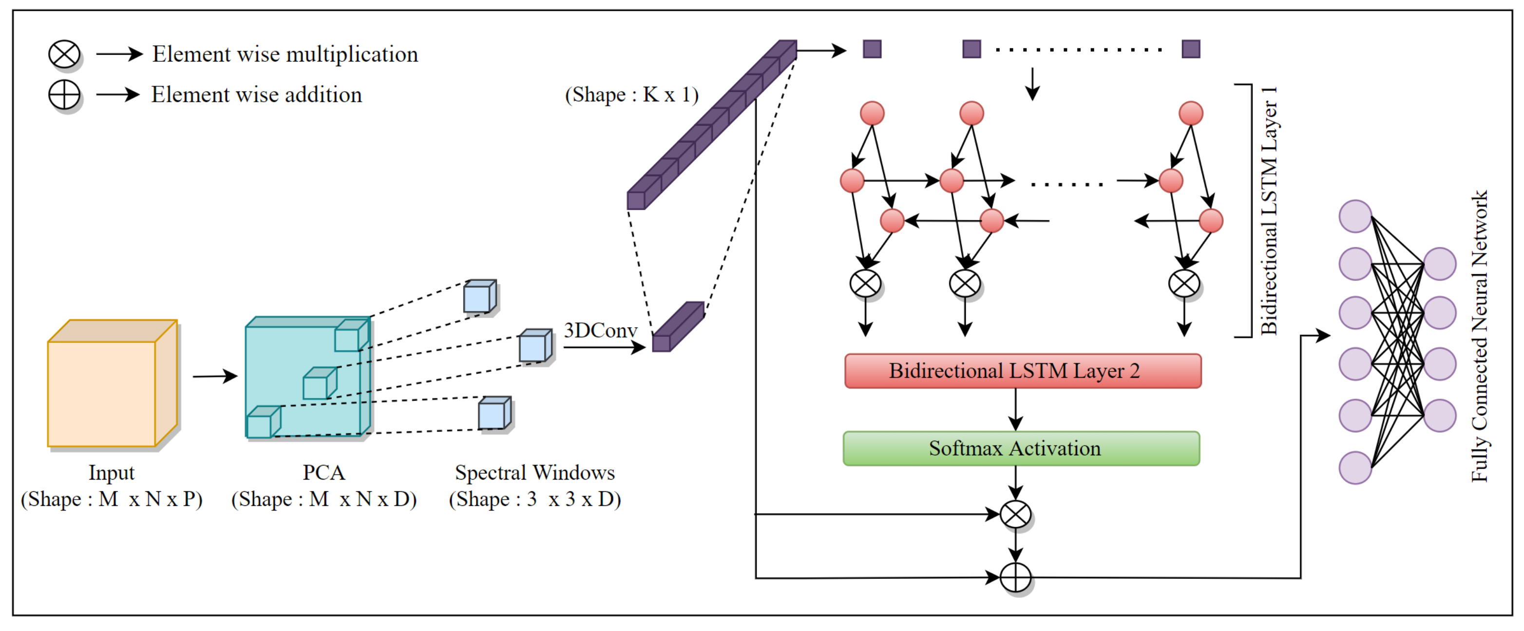
Hence, in the proposed data analysis framework, PCA is employed as a DR technique to reduce the spectral dimension of the input raw hyperspectral data cube. PCA is used to project a high dimensional hyperspectral data to its lower dimensional feature space to preserve crucial information present in the data. It also directly provides DR benefits such as a reduction of inherent noise and redundant information present in the data. Consequently, an input hyperspectral data cube X of spatial dimensions and spectral dimension P is now dimensionally reduced to size . The proposed model then extracts 3D patches of pixels to preserve the spectral information from the input data in the shape of , on which a 3D convolution operation with 32 kernels of shape is applied to extract and preserve the corresponding local neighborhood interactions between pixels and their spectral correlation. The spatial dimension of the convolutional kernel was set to to make it experimentally less computationally expensive for the framework to convert a spatially windowed input to a spectral vector, which is the input to the bidirectional LSTM in the successive stage of the HSI analysis framework. However, the choice was not frantically made. The spatial size of and the spectral dimensional size of 30 for the 3D-convolutional kernel were empirically compared against many other choices and were chosen because they produced the best trade-off between computational efficacy and execution time during experimentation. This is followed by another convolution operation with 32 kernels of shape . As a result, the output from this function has a shape of .
Successively, this pixel vector is passed through a bidirectional LSTM-based spectral attention gating mechanism as described in Equations (1)–(5). This attention gating mechanism selectively emphasizes the relevant informative pixels and suppresses the irrelevant bands. For any time step t, given a minibatch input (n, number of samples; d, number of inputs in each example), and a hidden layer activation function , assuming that the forward and backward hidden states for this time step are and , respectively, where h is the number of hidden units, the mathematical representation of the attention gating mechanism is illustrated below.
Next, we obtain the final hidden state output by multiplying and as shown in Equation (1). The same operations described in Equations (1)–(3) are repeated twice before the final output of the attention gating mechanism is obtained as shown in Equations (4) and (5).
The softmax activation function has been used on the output of the second bidirectional LSTM layer. The output of this softmax activation produces an activation map (which consists of probabilities ranging between 0 and 1), which directly reflects the importance of the output features. These probabilities are then multiplied with the output of the 3D convolution layer, which affects the weighting of the individual pixels in the -shaped input vector by selectively emphasizing the pixels that contain more information and suppressing the ones with less information.
These constructed features are now used as an input for an FNN with 3 layers of 100, 50, and C nodes, respectively, with a dropout of 0.2 between the first two dense layers for supervised classification. Here, C denotes the number of classes in the dataset. The overall 3D-convolution and bidirectional LSTM-based spectral attention and classification framework—BI-DI-SPEC-ATTN—is illustrated in Figure 1.
3. Methodologies for Comparison
3.1. PCA-3D-CNN
The PCA-3D-CNN deep learning methodology is considered to understand the effects of a spectral-only feature extraction framework, wherein a conventional DR technique such as PCA is used in tandem with supervised classification using CNN for hyperspectral data analysis. The emphasis here is to understand the effect of CNN-based conventional spectral feature extraction techniques such as PCA on hyperspectral data analysis. In this approach, the hyperspectral data in its original dimensionality P is projected onto a D-dimensional subspace using PCA for the spectral feature extraction. The resultant low-dimensional data are windowed into a size of (3 × 3 × D) followed by a 3D-CNN model for supervised classification. All the network parameters were empirically estimated for optimal results [6]. In the PCA-3D-CNN model, the first layer is a 3D-convolutional layer with 16 filters with dimension (3 × 3 × 32) followed by a flatten layer that is carried forward into an FNN with 100, 50, and C nodes with a dropout between every two layers with a value of 0.2, where C denotes the number of classes in the dataset.
3.2. SPEC-3D-CNN
Convolutions in a 2D-CNN can only capture 2-dimensional spatial information, and disregard the information along the spectral/temporal dimension. To address this concern, Ji et al. extended the idea of 2D-CNN used for 2D images to a 3D convolution in both space (2D) and time for video classification [33] and this acted as an inspiration for the HSI data classification methodology SPEC-3D-CNN. This methodology is identical to PCA-3D-CNN in its motivation to understand the contribution of spectral features exclusively on the proposed hyperspectral data analysis framework. However, unlike PCA-3D-CNN, there is no DR or spectral feature extraction technique employed on the original hyperspectral data. Here, the hyperspectral data in its original spectral dimensions P are directly introduced to the 3D-CNN classification architecture discussed in Section 3.1. This implies that the shape of the input to the 3D-CNN in the SPEC-3D-CNN methodology is (3 × 3 × P). This SPEC-3D-CNN model was specifically considered to study the effects of DR techniques or lack thereof on the automation performance of hyperspectral data analysis.
3.3. SPAT-2D-CNN
The aim of this model is to understand the contribution of spatial information alone on the CNN architecture. In this exclusive spatial feature extraction methodology, spatial contextual information is exploited by constructing features for a data point around its spatial neighborhood with the aid of 2D convolutional kernels. In this model, a (3 × 3) spatial neighborhood is considered, which is consistent with the other comparison methodologies defined in Section 3. This windowed data are now introduced as inputs to a 2D-CNN-based classification architecture. All CNN model hyperparameters and layers were empirically estimated for best performance. As in the SPEC-3D-CNN architecture, no DR technique was used on the original hyperspectral data in this SPAT-2D-CNN framework.
3.4. SVM-CK
In this work, we validate our proposed CNN architectures against the traditional composite kernel SVM (SVM-CK) for an inclusive spatial–spectral information extraction framework. The spatial features are extracted by calculating the spatial mean over a (3 × 3) window surrounding the pixel under consideration and its corresponding linear spatial kernel is computed [4,23]. Whereas for spectral features, the hyperspectral pixel vectors are directly used as spectral feature vector and RBF is used as the spectral kernel. Thus, the SVM-CK model incorporates both spatial and spectral features present in the hyperspectral data to provide enhanced classification performance. All the experiments related to the SVM-CK-model-based hyperspectral classification were conducted using LIBSVM on raw hyperspectral data without the use of any dimensionality reduction technique.
4. Experimental Results
In this section, all the datasets used for experimentation are briefly discussed alongside a detailed report on the experimental setup used for all the experiments conducted in this research work. Additionally, the efficiency of the proposed spectral attention and classification architecture BI-DI-SPEC-ATTN is validated and compared against four other models namely, PCA-3D-CNN, SPEC-3D-CNN, SPAT-2D-CNN, and SVM-CK as described in Section 3.
4.1. Datasets
All experiments were conducted on two airborne visible/infrared imaging spectrometer (AVIRIS) datasets—Salinas and Indian Pines—and a reflective optics system imaging spectrometer (ROSIS) dataset—University of Pavia [34]. The Salinas dataset is composed of 224 spectral bands, out of which 20 water absorption bands have been discarded. It has a spatial resolution of (512 × 217). This dataset comprises 16 classes related to vegetables, vineyard fields, and bare soils. The Indian Pines dataset was acquired by an AVIRIS sensor over the Indian Pines test site in northwestern Indiana. This dataset has a spatial dimension of 145 × 145 and 224 spectral bands (200 after removal of the water-absorption bands) with a spatial resolution of 20 m spanning 16 land cover classes. The Pavia University dataset has 103 spectral bands each having a spatial dimension of (610 × 340) with a spatial resolution of 1.3 m spanning nine classes of land covers. For each dataset, the training set was randomly chosen spanning from 5% through 50%.
4.2. Parameter Tuning and Experimental Setup
For our proposed methodology to function optimally, we have several parameters that need to be adjusted: the size of the reduced dimensional space using DR (D), the learning rate, the optimizer, etc. The reduced dimension D for the PCA computation was empirically found to be 100 for the Salinas and Indian Pines datasets and 50 for the Pavia University datasets, respectively. The length of the LSTM input vector K was empirically set to 256 for the Salinas and Indian Pines datasets and 128 for the Pavia University dataset, respectively. All parameters in the proposed approach were experimentally set to their optimal values to produce the best classification results. These parameters related to both the proposed methodology and frameworks used for comparison were tuned well enough to not leave any room for improvement for the classification results on all three datasets.
The objective function used in all our experimentation was the categorical cross-entropy with a learning rate of and a decay of . The choice to pick categorical cross-entropy as the objective function was straightforward, as the nature of the problem we address in this work is multiclass classification. However, this was not the case when choosing an optimal learning rate during experimentation. Numerous values of learning rates, such as , , , , , and were investigated. Upon rigorous experimentation, it was determined that a learning rate of with a decay of produced optimal results on all three datasets, and fluctuated the least when the results were averaged over three trials. Additionally, choosing a suitable batch size can effectively improve the memory utilization while training the classification model and improve the convergence accuracy of the architecture. We experimented by setting the batch size to multiple values, namely, 16, 32, 64, and 128, with a batch size of 32 producing the optimal results on all three datasets.
All the experiments used the Adam optimizer as it produced optimum results on all the datasets that are discussed in this work. In a normal gradient descent optimizer, the weights are adjusted based on the gradient calculated in the same epoch. However, with the Adam optimizer, the weights are adjusted based on the moving average of gradients calculated in current and previous epochs. The moments adjustment as per the Adam algorithm is calculated as a moving average of previous and current gradients and then those moments are used to update the weights. Gradient descent, RMSprop, and Adam optimizers, which are well known in the literature, were pitted against each other during experimentation and the Adam optimizer produced the best classification results on the Salinas, Indian Pines and Pavia University datasets.
To avoid any bias induced by random sampling of pixels, the classification results were averaged over three trials and the average accuracies along with execution time of the models are presented. All experiments were implemented using python on an Intel(R) Core(TM) i7-7700HQ processor with 16 GB RAM machine, and no GPU training was involved. For the purpose of training on all three datasets, samples were picked randomly from each class label in equal proportion and experimental results across different train/test ratios spanning from 5% through 50% were documented.
4.3. Discussion
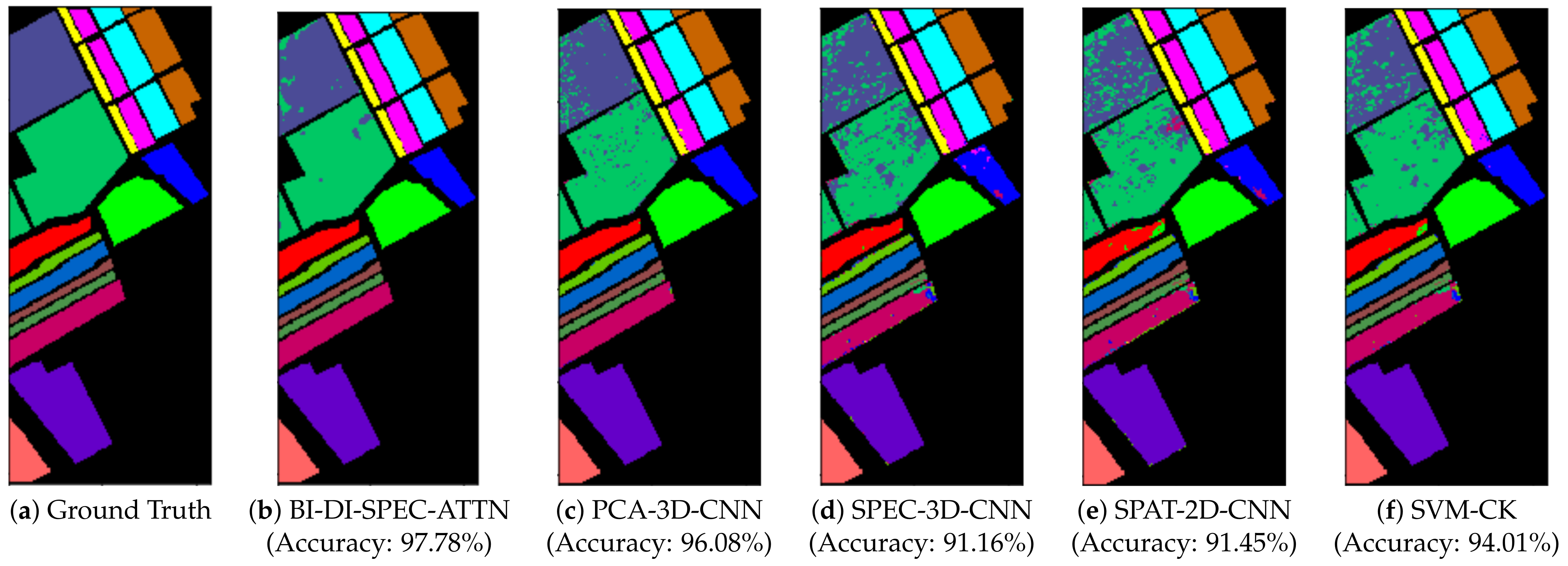
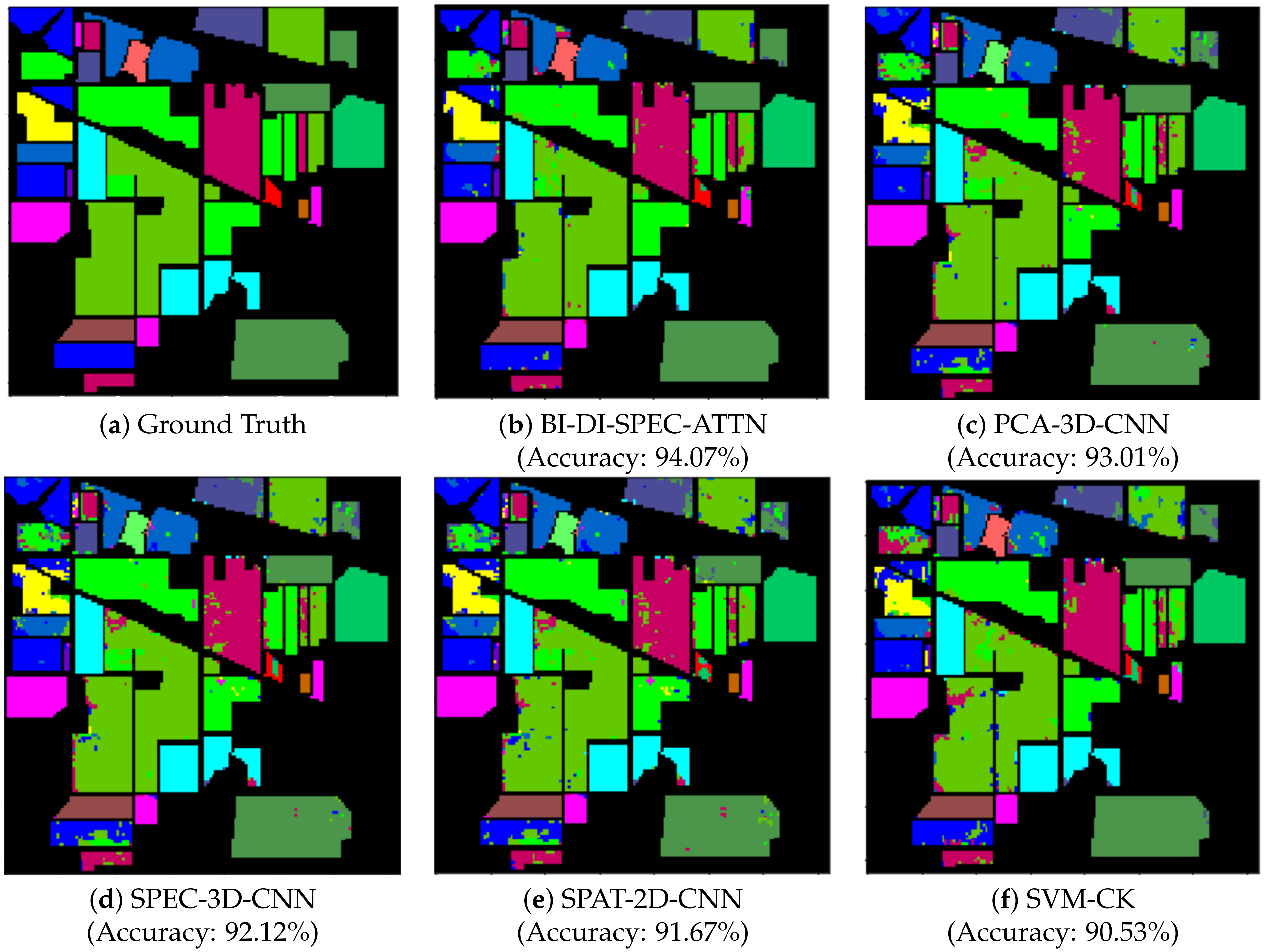
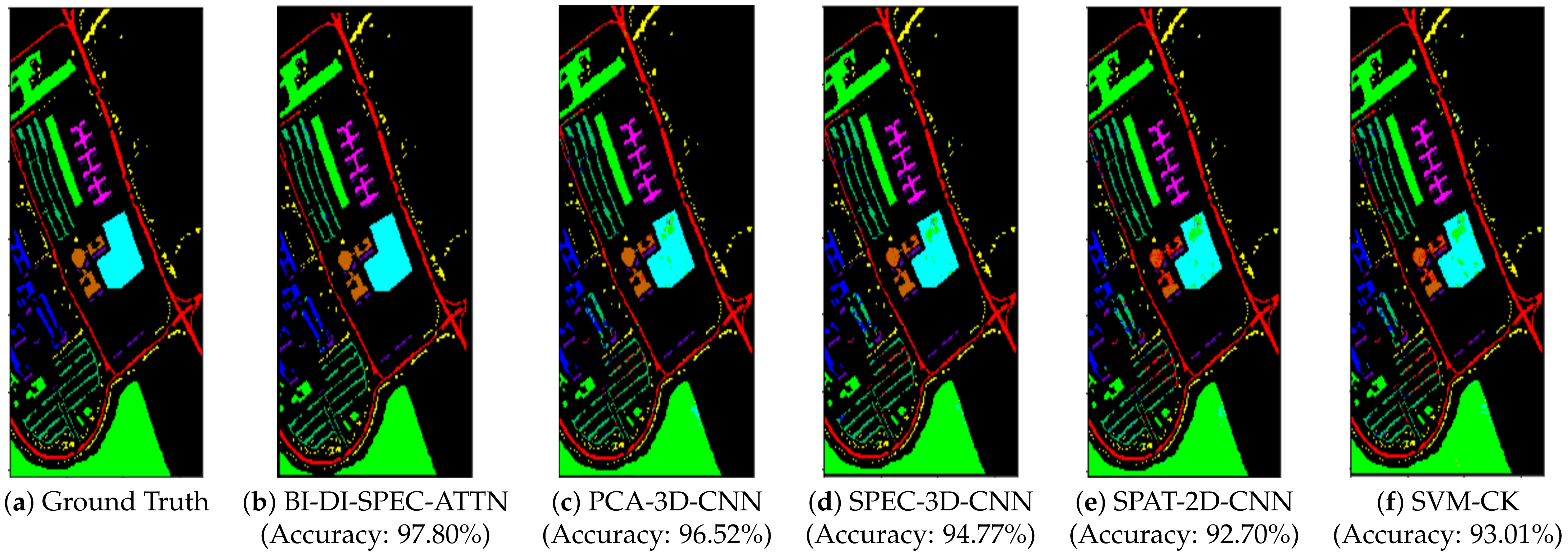
Table 1, Table 2 and Table 3 denote the specific number of training and testing samples used for experimentation with 10% of training data across all three datasets discussed in this paper. Figure 2, Figure 3 and Figure 4 illustrate the classification maps for of training data for the proposed bidirectional LSTM-based spectral attention and classification analysis methodology BI-DI-SPEC-ATTN for the Salinas, Indian Pines, and Pavia University datasets, along with the frameworks used for comparison. It can be further inferred from Table 4, Table 5 and Table 6 that BI-DI-SPEC-ATTN gave superior classification performance over other frameworks that are discussed for both the Indian Pines and Pavia University datasets. Table 7 shows the overall execution time of all the models in this work for 10% of training data. It can be clearly noted from Figure 2, Figure 3 and Figure 4 that our proposed BI-DI-SPEC-ATTN methodology has more coherent classification regions and fewer misclassifications with a competitive computational efficiency when compared to other methods discussed, at a reasonable trade-off between computational time and classification performance compared to other spatial-only, spectral-only and spatial–spectral-information-based feature extraction models.
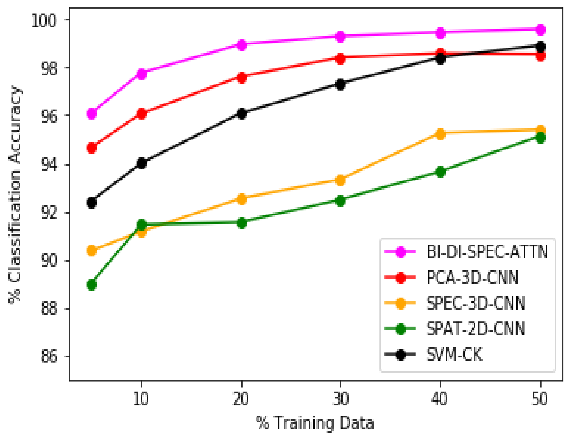
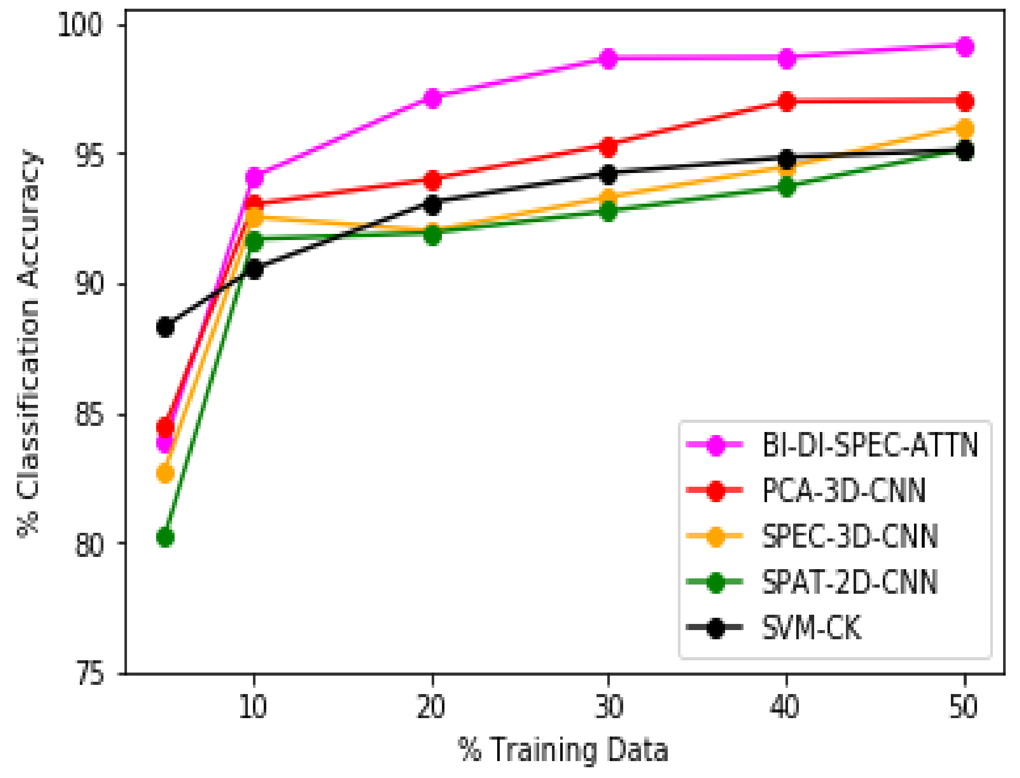
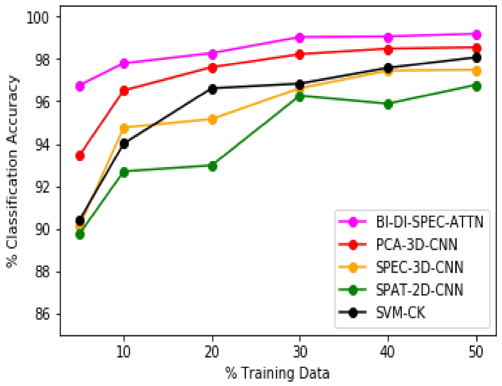
Our proposed framework produces the best classification results with an overall accuracy of 97.78%, 94.07%, and 97.80% on the Salinas, Indian Pines, and Pavia University datasets, respectively, for just 10% of training samples selected, which can be reaffirmed from the figures and tables documented in Section 4. Even though other classification methodologies discussed in this work are efficient, with many of them being state-of-the-art techniques, they lack the ability to capture distinctive features and information between different classes across the three datasets discussed in this work to produce effective classification results in comparison with the proposed BI-DI-SPEC-ATTN methodology. While the state-of-the-art composite kernel SVM-based classification technique (SVM-CK) discussed produced good classification results on the Salinas and Pavia University datasets with its ability to incorporate both spatial and spectral features present in the hyperspectral data through a 3 × 3 window-based average spatial kernel, coupled with an RBF spectral kernel, it under-performs when applied on the Indian Pines dataset, producing larger misclassification regions compared to all the other methodologies. Additionally, the 3D-CNN-based classification methodologies discussed in our work, namely, PCA-3D-CNN and SPEC-3D-CNN, produced superior classification results overall against their counterparts, namely, the 2D-CNN-architecture-based classification techniques SPAT-2D-CNN and SVM-CK, owing to their ability to effectively incorporate both spatial and temporal features that are critical for effective classification of hyperspectral data. Finally, the results produced by the proposed bidirectional LSTM-based attention and classification framework outperformed all the methodologies discussed in this work demonstrating the importance and feasibility of constructing the relationship between features and weighing them with the aid of an effective attention methodology. This was followed by a solid FNN-based network for classification of the constructed features, which produced results that bolstered the efficacy of the proposed technique.
The efficacy of our proposed methodology BI-DI-SPEC-ATTN can be further affirmed from the overall classification accuracy plots as depicted in Figure 5, Figure 6 and Figure 7 for the Salinas, Indian Pines, and Pavia University datasets, respectively. Our proposed approach BI-DI-SPEC-ATTN significantly outperformed all other methods compared, especially against the conventional principal-component-analysis-based spectral feature analysis model (PCA-3D-CNN), a 2D-convolutional-neural-network-based hyperspectral data classification model (SPAT-2D-CNN) and a conventionally used SVM-based spatial–spectral information inclusion model (SVM-CK). Our proposed methodology BI-DI-SPEC-ATTN presents a pragmatic and an efficient attention-based classification framework to automate the feature selection process through varied levels of importance/weighting assigned to spectral bands in a dataset, based on their quality of information. Thus, the BI-DI-SPEC-ATTN model provides superior classification performance not only with just of training samples but also at various different training-testing ratios as demonstrated above in Figure 5, Figure 6 and Figure 7. Therefore, our BI-DI-SPEC-ATTN model serves as an effective framework for automated decision making with excellent classification performance for hyperspectral data analysis applications.
With the wide range of experiments and analysis that we conducted, it would definitely be worthy to denote the importance of PCA as a dimensionality reduction technique alongside being a principal feature extraction component in our work. It not only reduced the computational complexity of our spectral attention and classification methodology (BI-DI-SPEC-ATTN), but also acted as an efficient lightweight spectral feature extraction technique and a noise reduction component.
The importance of a dimensionality reduction technique such as PCA for DR, information retrieval, and as a linear orthogonal transformation technique that transforms the data to a new coordinate system, has been justified in the literature over time in HSI applications. PCA is explicitly not designed for noise removal but instead, it is designed to reduce the dimensionality of the feature space with which the underlying deep learning regression/classification model approximates. We can think of PCA as a tuning knob to smoothly decide how much information we want to retain, which is impossible to achieve if one works directly with the original features. Since we cannot directly decide which features to retain and the ones to eliminate, as the original features have no order of priority or usability, PCA comes into play.
As a result, eliminating some of the PCs with lower variances, i.e., with lower eigenvalues, usually helps the model to generalize better. PCs with higher eigenvalues capture the principal information about the dataset and thus adding more and more PCs ends up appending information to the existing reduced dimensional data space. Thus, removing some PCs with lower eigenvalues actually acts as a regularization technique to minimize the redundancy of the information present in the data. Hence, in this work, we aimed to alleviate the inherent process noise and data redundancy present in the hyperspectral data using PCA to enhance the data learning outcomes of deep learning methods [4,6].
Alongside PCA, the bidirectional LSTM-based feature importance weighting/attention module, which operates by selectively emphasizing the feature values and correlating the output sequence of feature vectors of the high dimensional hyperspectral data with the results of selective learning, constitutes our proposed attention and classification framework BI-DI-SPEC-ATTN.
Additionally, Table 7 denotes the overall execution time (includes training, validation, and testing) for all the methodologies discussed in this work for the Salinas, Indian Pines and Pavia University datasets with 10% of training data. Overall, the experimental results presented in this paper demonstrate that the proposed bidirectional and 3D-CNN-oriented spectral-attention-based classification architecture (BI-DI-SPEC-ATTN) required only a small number of training samples for effective classification, while also providing robust performance with all the datasets used in the experimentation phase.
5. Conclusions
In this work, a novel deep-learning-based bidirectional spectral attention and classification mechanism was introduced. Compared to the traditional deep-learning-based hyperspectral data analysis approaches, our work explores the ability of a gated spectral attention mechanism to adaptively diversify spectral bands by selectively emphasizing the more informative bands and suppressing the less useful ones for a superior classification performance. Experimental results demonstrated that the proposed BI-DI-SPEC-ATTN methodology yielded outstanding classification performance while being robust under a limited training samples scenario, when compared to other spatial- and spectral-only based feature extraction and classification approaches. Our spectral attention based hyperspectral data analysis framework, BI-DI-SPEC-ATTN, further illustrated the efficacy and potential to learn and prioritize features in the high-dimensional HSI data and extract important relationships between the spectral features, which reinforced the goal of effective and efficient automation in hyperspectral remote sensing applications.
Author Contributions
Conceptualization, B.P. and V.M.; methodology, B.P.; software, B.P.; validation, B.P. and V.M.; formal analysis, B.P. and V.M.; investigation, B.P.; resources, B.P.; data curation, B.P.; writing—original draft preparation, B.P. and V.M.; writing—review and editing, V.M.; visualization, B.P.; supervision, V.M.; project administration, V.M.; funding acquisition, V.M. All authors have read and agreed to the published version of the manuscript.
Funding
Publication costs was supported by an Early Career Research Fellowship from the Gulf Research Program of the National Academies of Sciences, Engineering, and Medicine.
Data Availability Statement
Statistical and computational models used are fully detailed in the main text. All datasets used are publicly available at: http://www.ehu.eus/ccwintco/index.php/Hyperspectral_Remote_Sensing_Scenes; accessed on 20 November 2021.
Acknowledgments
This research work was supported by an Early Career Research Fellowship from the Gulf Research Program of the National Academies of Sciences, Engineering, and Medicine. DISCLAIMER: “The content is solely the responsibility of the authors and does not necessarily represent the official views of the Gulf Research Program of the National Academies of Sciences, Engineering, and Medicine.”
Conflicts of Interest
The authors declare no conflict of interest.
References
- Weng, Q. (Ed.) Advances in Environmental Remote Sensing: Sensors, Algorithms, and Applications; CRC Press: Boca Raton, FL, USA, 2011. [Google Scholar]
- Chen, Y.; Jiang, H.; Li, C.; Jia, X.; Ghamisi, P. Deep feature extraction and classification of hyperspectral images based on convolutional neural networks. IEEE Trans. Geosci. Remote Sens. 2016, 54, 6232–6251. [Google Scholar]
- Gao, Q.; Lim, S.; Jia, X. Hyperspectral Image Classification using Convolutional Neural Networks and Multiple Feature Learning. Remote Sens. 2018, 10, 299. [Google Scholar]
- Praveen, B.; Menon, V. Novel deep-learning-based spatial-spectral feature extraction for hyperspectral remote sensing applications. In Proceedings of the 2019 IEEE International Conference on Big Data (Big Data), Los Angeles, CA, USA, 9–12 December 2019; pp. 5444–5452. [Google Scholar]
- Mou, L.; Ghamisi, P.; Zhu, X.X. Deep recurrent neural networks for hyperspectral image classification. IEEE Trans. Geosci. Remote Sens. 2017, 55, 3639–3655. [Google Scholar]
- Praveen, B.; Menon, V. A Study of Spatial-Spectral Feature Extraction frameworks with 3D Convolutional Neural Network for Robust Hyperspectral Imagery Classification. IEEE J. Sel. Top. Appl. Earth Obs. Remote Sens. 2020, 14, 1717–1727. [Google Scholar]
- Foster, K.; Menon, V. A Study of Spatial-Spectral Information Fusion Methods in the Artificial Neural Network Paradigm for Hyperspectral Data Analysis in Swarm Robotics Applications. In Proceedings of the 2019 SoutheastCon, Huntsville, AL, USA, 11–14 April 2019; pp. 1–8. [Google Scholar]
- Huo, H.; Guo, J.; Li, Z.L. Hyperspectral image classification for land cover based on an improved interval type-II fuzzy C-means approach. Sensors 2018, 18, 363. [Google Scholar]
- Chen, Z.; Jiang, J.; Jiang, X.; Fang, X.; Cai, Z. Spectral-spatial feature extraction of hyperspectral images based on propagation filter. Sensors 2018, 18, 1978. [Google Scholar]
- Bui, Q.T.; Nguyen, Q.H.; Pham, V.M.; Pham, V.D.; Tran, M.H.; Tran, T.T.; Nguyen, H.D.; Nguyen, X.L.; Pham, H.M. A novel method for multispectral image classification by using social spider optimization algorithm integrated to fuzzy C-mean clustering. Can. J. Remote Sens. 2019, 45, 42–53. [Google Scholar]
- Hsu, P.H.; Tseng, Y.H.; Gong, P. Spectral feature extraction of hyperspectral images using wavelet transform. ISPRS J. Photogramm. Remote Sens. 2006, 11, 93–109. [Google Scholar]
- Sun, H.; Ren, J.; Zhao, H.; Sun, G.; Liao, W.; Fang, Z.; Zabalza, J. Adaptive distance-based band hierarchy (ADBH) for effective hyperspectral band selection. IEEE Trans. Cybern. 2020, 1–13. [Google Scholar] [CrossRef] [Green Version]
- Huang, K.; Li, S.; Kang, X.; Fang, L. Spectral–spatial hyperspectral image classification based on KNN. Sens. Imaging 2016, 17, 1. [Google Scholar]
- Peng, J.; Li, L.; Tang, Y.Y. Maximum likelihood estimation-based joint sparse representation for the classification of hyperspectral remote sensing images. IEEE Trans. Neural Netwo. Learn. Syst. 2018, 30, 1790–1802. [Google Scholar]
- Li, J.; Bioucas-Dias, J.M.; Plaza, A. Semisupervised hyperspectral image segmentation using multinomial logistic regression with active learning. IEEE Trans. Geosci. Remote Sens. 2010, 48, 4085–4098. [Google Scholar]
- Ham, J.; Chen, Y.; Crawford, M.M.; Ghosh, J. Investigation of the random forest framework for classification of hyperspectral data. IEEE Trans. Geosci. Remote Sens. 2005, 43, 492–501. [Google Scholar]
- Li, L.; Wang, C.; Li, W.; Chen, J. Hyperspectral image classification by AdaBoost weighted composite kernel extreme learning machines. Neurocomputing 2018, 275, 1725–1733. [Google Scholar]
- Köppen, M. The curse of dimensionality. In Proceedings of the 5th Online World Conference on Soft Computing in Industrial Applications, Online, 4–18 September 2000; Volume 1, pp. 4–8. [Google Scholar]
- Khodr, J.; Younes, R. Dimensionality reduction on hyperspectral images: A comparative review based on artificial datas. In Proceedings of the 2011 4th International Congress on Image and Signal Processing, Shanghai, China, 15–17 October 2011; Volume 4, pp. 1875–1883. [Google Scholar]
- Jolliffe, I.T. Principal Component Analysis; Springer: New York, NY, USA, 1986; pp. 129–155. [Google Scholar]
- Duda, R.O.; Hart, P.E.; Stork, D.G. Pattern Classification, 2nd ed.; John Wiley and Sons: New York, NY, USA, 2001; pp. 517–598. [Google Scholar]
- Menon, V.; Du, Q.; Christopher, S. Improved Random Projection with K-Means Clustering for Hyperspectral Image Classification. In Proceedings of the 2018 IEEE International Geoscience and Remote Sensing Symposium, Valencia, Spain, 22–27 July 2018; pp. 4768–4771. [Google Scholar]
- Menon, V.; Prasad, S.; Fowler, J.E. Hyperspectral classification using a composite kernel driven by nearest-neighbor spatial features. In Proceedings of the IEEE International Conference on Image Processing (ICIP), Quebec City, QC, Canada, 27–30 September 2015; pp. 2100–2104. [Google Scholar]
- Li, J.; Marpu, P.R.; Plaza, A.; Bioucas-Dias, J.M.; Benediktsson, J.A. Generalized composite kernel framework for hyperspectral image classification. IEEE Trans. Geosci. Remote Sens. 2013, 51, 4816–4829. [Google Scholar]
- Valero, O.; Salembier, P.; Chanussot, J. Object recognition in urban hyperspectral images using Binary PartitionTree representation. In Proceedings of the IEEE International Geoscience and RemoteSensing Symposium—IGARSS, Melbourne, Australia, 21–26 July 2013; pp. 4098–4101. [Google Scholar]
- Li, R.; Zheng, S.; Duan, C.; Yang, Y.; Wang, X. Classification of Hyperspectral Image Based on Double-Branch Dual-Attention Mechanism Network. Remote Sens. 2020, 12, 582. [Google Scholar]
- Mou, L.; Zhu, X.X. Learning to Pay Attention on Spectral Domain: A Spectral Attention Module-Based Convolutional Network for Hyperspectral Image Classification. IEEE Trans. Geosci. Remote Sens. 2020, 58, 110–122. [Google Scholar]
- Gao, L.R.; Zhang, B.; Zhang, X.; Zhang, W.J.; Tong, Q.X. A new operational method for estimating noise in hyperspectral images. IEEE Geosci. Remote Sens. Lett. 2008, 5, 83–87. [Google Scholar]
- Uddin, M.P.; Mamun, M.A.; Hossain, M.A. Feature extraction for hyperspectral image classification. In Proceedings of the IEEE Region 10 Humanitarian Technology Conference, Dhaka, Bangladesh, 21–23 December 2017; pp. 379–382. [Google Scholar]
- Ardakani, A.; Condo, C.; Ahmadi, M.; Gross, W.J. An architecture to accelerate convolution in deep neural networks. IEEE Trans. Circuits Syst. I Regul. Pap. 2017, 65, 1349–1362. [Google Scholar]
- Graves, A.; Fernández, S.; Schmidhuber, J. Bidirectional LSTM networks for improved phoneme classification and recognition. In Proceedings of the International Conference on Artificial Neural Networks, Palma de Mallorca, Spain, 10–12 June 2005; pp. 799–804. [Google Scholar]
- Fine, T.L. Feedforward Neural Network Methodology; Springer Science and Business Media: Berlin, Germany, 2006. [Google Scholar]
- Ji, S.; Xu, W.; Yang, M.; Yu, K. 3D convolutional neural networks for human action recognition. IEEE Trans. Pattern Anal. Mach. Intell. 2012, 35, 221–231. [Google Scholar]
- Gamba, P. A collection of data for urban area characterization. In Proceedings of the IEEE International Geo-science and Remote Sensing Symposium, Anchorage, AK, USA, 20–24 September 2004. [Google Scholar]
Figure 1.
The proposed 3D-convolution and bidirectional LSTM-based attention and classification architecture (BI-DI-SPEC-ATTN).
Figure 1.
The proposed 3D-convolution and bidirectional LSTM-based attention and classification architecture (BI-DI-SPEC-ATTN).

Figure 2.
Classification maps of Salinas dataset for all proposed methodologies using 10% of training data.
Figure 2.
Classification maps of Salinas dataset for all proposed methodologies using 10% of training data.

Figure 3.
Classification maps of Indian Pines dataset for all proposed methodologies using 10% of training data.
Figure 3.
Classification maps of Indian Pines dataset for all proposed methodologies using 10% of training data.

Figure 4.
Classification maps of Pavia University dataset for all proposed methodologies using 10% of training data.
Figure 4.
Classification maps of Pavia University dataset for all proposed methodologies using 10% of training data.

Figure 5.
Overall classification accuracies on Salinas dataset for varying sizes of training samples.
Figure 5.
Overall classification accuracies on Salinas dataset for varying sizes of training samples.

Figure 6.
Overall classification accuracies on Indian Pines dataset for varying sizes of training samples.
Figure 6.
Overall classification accuracies on Indian Pines dataset for varying sizes of training samples.

Figure 7.
Overall classification accuracies on Pavia University dataset for varying sizes of training samples.
Figure 7.
Overall classification accuracies on Pavia University dataset for varying sizes of training samples.


Table 1.
Total number of class-specific training and testing samples used for Salinas dataset with 10% of training data.
Table 1.
Total number of class-specific training and testing samples used for Salinas dataset with 10% of training data.
| # | Class Name | # of Training Samples | # of Testing Samples |
|---|---|---|---|
| 1 | Brocoli-green-weeds-1 | 200 | 1809 |
| 2 | Brocoli-green-weeds-2 | 372 | 3354 |
| 3 | Fallow | 198 | 1778 |
| 4 | Fallow-rough-plow | 140 | 1254 |
| 5 | Fallow-smooth | 268 | 2410 |
| 6 | Stubble | 396 | 3563 |
| 7 | Celery | 358 | 3221 |
| 8 | Grapes-untrained | 1128 | 10,143 |
| 9 | Soil-vinyard-develop | 620 | 5583 |
| 10 | Corn-senesced-green-weeds | 328 | 2950 |
| 11 | Lettuce-romaine-4wk | 106 | 962 |
| 12 | Lettuce-romaine-5wk | 192 | 1735 |
| 13 | Lettuce-romaine-6wk | 92 | 824 |
| 14 | Lettuce-romaine-7wk | 108 | 962 |
| 15 | Vinyard-untrained | 726 | 6542 |
| 16 | Vinyard-vertical-trellis | 180 | 1627 |
| Total | 5412 | 48,717 |
Table 2.
Total number of class-specific training and testing samples used for Indian Pines dataset with 10% of training data.
Table 2.
Total number of class-specific training and testing samples used for Indian Pines dataset with 10% of training data.
| # | Class Name | # of Training Samples | # of Testing Samples |
|---|---|---|---|
| 1 | Alfalfa | 5 | 41 |
| 2 | Corn-notill | 140 | 1288 |
| 3 | Corn-mintill | 81 | 749 |
| 4 | Corn | 24 | 213 |
| 5 | Grass-pasture | 48 | 435 |
| 6 | Grass-trees | 72 | 658 |
| 7 | Grass-pasture-mowed | 3 | 25 |
| 8 | Hay-Windrowed | 47 | 431 |
| 9 | Oats | 2 | 18 |
| 10 | Soybean-notill | 95 | 877 |
| 11 | Soybean-mintill | 232 | 2223 |
| 12 | Soybean-clean | 58 | 535 |
| 13 | Wheat | 21 | 184 |
| 14 | Woods | 124 | 1141 |
| 15 | Buildings-Grass-Trees-Drives | 38 | 348 |
| 16 | Stone-Steel-Towers | 10 | 83 |
| Total | 1000 | 9249 |
Table 3.
Total number of class-specific training and testing samples used for University of Pavia University dataset with 10% of training data.
Table 3.
Total number of class-specific training and testing samples used for University of Pavia University dataset with 10% of training data.
| # | Class Name | # of Training Samples | # of Testing Samples |
|---|---|---|---|
| 1 | Asphalt | 663 | 5968 |
| 2 | Meadows | 1865 | 16,784 |
| 3 | Gravel | 210 | 1889 |
| 4 | Trees | 306 | 2758 |
| 5 | Painted Metal Sheets | 134 | 1211 |
| 6 | Bare Soil | 503 | 4526 |
| 7 | Bitumen | 133 | 1197 |
| 8 | Self-Blocking Bricks | 368 | 3314 |
| 9 | Shadows | 95 | 852 |
| Total | 4277 | 38,499 |
Table 4.
Class-specific accuracies of Indian Pines dataset with 10% of training data for the proposed methodology and other models used for comparison.
Table 4.
Class-specific accuracies of Indian Pines dataset with 10% of training data for the proposed methodology and other models used for comparison.
| # | Class Name | BI-DI-SPEC-ATTN | PCA-3D-CNN | SPEC-3D-CNN | SPAT-2D-CNN | SVM-CK |
|---|---|---|---|---|---|---|
| 1 | Alfalfa | 86.1 | 54.9 | 98.8 | 83.8 | 92.6 |
| 2 | Corn-notill | 94.2 | 93.6 | 93.2 | 81.7 | 92.4 |
| 3 | Corn-mintill | 83.3 | 93.0 | 85.6 | 79.3 | 92.5 |
| 4 | Corn | 92.1 | 82.8 | 86.9 | 78.4 | 91.0 |
| 5 | Grass-pasture | 94.3 | 92.7 | 93.7 | 95.8 | 92.3 |
| 6 | Grass-trees | 97.8 | 99.5 | 96.1 | 97.7 | 83.1 |
| 7 | Grass-pasture-mowed | 57.8 | 79.1 | 95.8 | 88.9 | 95.4 |
| 8 | Hay-Windrowed | 99.4 | 95.2 | 94.3 | 97.5 | 90.0 |
| 9 | Oats | 68.3 | 75.9 | 72.2 | 53.6 | 89.1 |
| 10 | Soybean-notill | 95.8 | 93.9 | 92.0 | 82.4 | 92.4 |
| 11 | Soybean-mintill | 92.1 | 96.8 | 93.2 | 84.8 | 94.3 |
| 12 | Soybean-clean | 95.6 | 89.2 | 95.8 | 95.7 | 87.5 |
| 13 | Wheat | 98.4 | 98.1 | 94.1 | 95.6 | 96.0 |
| 14 | Woods | 97.8 | 95.7 | 94.8 | 86.1 | 92.2 |
| 15 | Buildings-Grass-Trees-Drives | 98.3 | 93.2 | 92.0 | 82.4 | 93.7 |
| 16 | Stone-Steel-Towers | 93.6 | 92.7 | 88.4 | 95.6 | 93.9 |
| OA (%) | 94.07 | 93.01 | 92.12 | 91.67 | 90.53 | |
| (%) | 94.03 | 92.87 | 91.54 | 90.88 | 90.17 |
Table 5.
Class-specific accuracies of Pavia University dataset with 10% of training data for the proposed methodology and other models used for comparison.
Table 5.
Class-specific accuracies of Pavia University dataset with 10% of training data for the proposed methodology and other models used for comparison.
| # | Class Name | BI-DI-SPEC-ATTN | PCA-3D-CNN | SPEC-3D-CNN | SPAT-2D-CNN | SVM-CK |
|---|---|---|---|---|---|---|
| 1 | Asphalt | 98.0 | 96.1 | 93.1 | 90.2 | 93.6 |
| 2 | Meadows | 98.9 | 97.8 | 97.0 | 88.1 | 96.4 |
| 3 | Gravel | 94.8 | 89.3 | 80.2 | 77.3 | 88.9 |
| 4 | Trees | 97.7 | 95.1 | 96.5 | 94.7 | 92.7 |
| 5 | Painted Metal Sheets | 99.0 | 97.8 | 98.2 | 88.9 | 98.3 |
| 6 | Bare Soil | 98.7 | 97.5 | 91.8 | 95.3 | 97.4 |
| 7 | Bitumen | 95.5 | 96.4 | 90.5 | 91.5 | 96.1 |
| 8 | Self-Blocking Bricks | 94.4 | 92.4 | 83.5 | 90.6 | 91.4 |
| 9 | Shadows | 95.8 | 94.2 | 97.8 | 94.9 | 95.3 |
| OA (%) | 97.80 | 96.52 | 94.77 | 92.70 | 93.01 | |
| (%) | 96.55 | 95.71 | 93.66 | 91.49 | 92.88 |
Table 6.
Class-specific accuracies of Salinas dataset with 10% of training data for the proposed methodology and other models used for comparison.
Table 6.
Class-specific accuracies of Salinas dataset with 10% of training data for the proposed methodology and other models used for comparison.
| # | Class Name | BI-DI-SPEC-ATTN | PCA-3D-CNN | SPEC-3D-CNN | SPAT-2D-CNN | SVM-CK |
|---|---|---|---|---|---|---|
| 1 | Brocoli-green-weeds-1 | 89.4 | 60.9 | 96.3 | 82.9 | 95.6 |
| 2 | Brocoli-green-weeds-2 | 97.5 | 96.9 | 92.1 | 82.1 | 94.3 |
| 3 | Fallow | 86.6 | 96.3 | 83.4 | 80.1 | 94.7 |
| 4 | Fallow-rough-plow | 95.4 | 85.0 | 84.6 | 79.5 | 95.2 |
| 5 | Fallow-smooth | 97.6 | 95.1 | 91.5 | 93.6 | 93.5 |
| 6 | Stubble | 99.1 | 99.8 | 94.7 | 95.1 | 86.8 |
| 7 | Celery | 60.2 | 83.4 | 93.6 | 85.7 | 96.5 |
| 8 | Grapes-untrained | 99.9 | 98.5 | 92.1 | 98.2 | 93.9 |
| 9 | Soil-vinyard-develop | 69.9 | 78.2 | 70.1 | 58.9 | 92.6 |
| 10 | Corn-senesced-green-weeds | 96.4 | 96.1 | 90.8 | 81.1 | 92.8 |
| 11 | Lettuce-romaine-4wk | 96.6 | 99.9 | 91.4 | 83.9 | 95.7 |
| 12 | Lettuce-romaine-5wk | 98.9 | 92.7 | 93.5 | 94.6 | 90.3 |
| 13 | Lettuce-romaine-6wk | 99.7 | 98.8 | 92.7 | 95.0 | 98.4 |
| 14 | Lettuce-romaine-7wk | 99.1 | 98.3 | 92.5 | 85.5 | 95.8 |
| 15 | Vinyard-untrained | 99.9 | 96.3 | 90.0 | 84.7 | 96.8 |
| 16 | Vinyard-vertical-trellis | 96.3 | 95.6 | 86.4 | 96.2 | 91.9 |
| OA (%) | 97.78 | 96.08 | 91.16 | 91.45 | 94.01 | |
| (%) | 96.92 | 95.66 | 91.02 | 90.97 | 93.75 |
Table 7.
Overall execution time (in minutes) of all the models in comparison for 10% training data.
| Dataset (10% Training) | BI-DI-SPEC-ATTN | PCA-3D-CNN | SPEC-3D-CNN | SPAT-2D-CNN | SVM-CK |
|---|---|---|---|---|---|
| Time: 28.64 | Time: 7.51 | Time: 12.47 | Time: 6.19 | Time: 22.76 | |
| Salinas | # of Parameters: 179,118 | # of Parameters: 120,272 | # of Parameters: 135,340 | # of Parameters: 115,388 | |
| Epochs: 100 | Epochs: 80 | Epochs: 80 | Epochs: 80 | ||
| Time: 36.20 | Time: 5.27 | Time: 10.39 | Time: 6.55 | Time: 21.54 | |
| Pavia University | # of Parameters: 96,841 | # of Parameters: 80,569 | # of Parameters: 100,264 | # of Parameters: 89,128 | |
| Epochs: 120 | Epochs: 80 | Epochs: 80 | Epochs: 80 | ||
| Time: 15.94 | Time: 9.63 | Time: 14.98 | Time: 7.21 | Time: 27.11 | |
| Indian Pines | # of Parameters: 179,118 | # of Parameters: 120,272 | # of Parameters: 135,340 | # of Parameters: 115,388 | |
| Epochs: 100 | Epochs: 80 | Epochs: 80 | Epochs: 80 |
Publisher’s Note: MDPI stays neutral with regard to jurisdictional claims in published maps and institutional affiliations. |
© 2022 by the authors. Licensee MDPI, Basel, Switzerland. This article is an open access article distributed under the terms and conditions of the Creative Commons Attribution (CC BY) license (https://creativecommons.org/licenses/by/4.0/).
Share and Cite
MDPI and ACS Style
Praveen, B.; Menon, V. A Bidirectional Deep-Learning-Based Spectral Attention Mechanism for Hyperspectral Data Classification. Remote Sens. 2022, 14, 217. https://0-doi-org.brum.beds.ac.uk/10.3390/rs14010217
AMA Style
Praveen B, Menon V. A Bidirectional Deep-Learning-Based Spectral Attention Mechanism for Hyperspectral Data Classification. Remote Sensing. 2022; 14(1):217. https://0-doi-org.brum.beds.ac.uk/10.3390/rs14010217
Chicago/Turabian StylePraveen, Bishwas, and Vineetha Menon. 2022. "A Bidirectional Deep-Learning-Based Spectral Attention Mechanism for Hyperspectral Data Classification" Remote Sensing 14, no. 1: 217. https://0-doi-org.brum.beds.ac.uk/10.3390/rs14010217
Note that from the first issue of 2016, this journal uses article numbers instead of page numbers. See further details here.