Article

Image-Aided LiDAR Mapping Platform and Data Processing Strategy for Stockpile Volume Estimation

1
Lyles School of Civil Engineering, Purdue University, West Lafayette, IN 47907, USA
2
Indiana Department of Transportation Highway Operations, Indianapolis, IN 46204, USA
3
Indiana Department of Transportation Research and Development, West Lafayette, IN 47906, USA
*
Author to whom correspondence should be addressed.
Submission received: 20 November 2021 / Revised: 30 December 2021 / Accepted: 1 January 2022 / Published: 5 January 2022

Abstract

:
Stockpile quantity monitoring is vital for agencies and businesses to maintain inventory of bulk material such as salt, sand, aggregate, lime, and many other materials commonly used in agriculture, highways, and industrial applications. Traditional approaches for volumetric assessment of bulk material stockpiles, e.g., truckload counting, are inaccurate and prone to cumulative errors over long time. Modern aerial and terrestrial remote sensing platforms equipped with camera and/or light detection and ranging (LiDAR) units have been increasingly popular for conducting high-fidelity geometric measurements. Current use of these sensing technologies for stockpile volume estimation is impacted by environmental conditions such as lack of global navigation satellite system (GNSS) signals, poor lighting, and/or featureless surfaces. This study addresses these limitations through a new mapping platform denoted as Stockpile Monitoring and Reporting Technology (SMART), which is designed and integrated as a time-efficient, cost-effective stockpile monitoring solution. The novel mapping framework is realized through camera and LiDAR data-fusion that facilitates stockpile volume estimation in challenging environmental conditions. LiDAR point clouds are derived through a sequence of data collections from different scans. In order to handle the sparse nature of the collected data at a given scan, an automated image-aided LiDAR coarse registration technique is developed followed by a new segmentation approach to derive features, which are used for fine registration. The resulting 3D point cloud is subsequently used for accurate volume estimation. Field surveys were conducted on stockpiles of varying size and shape complexity. Independent assessment of stockpile volume using terrestrial laser scanners (TLS) shows that the developed framework had close to 1% relative error.

Graphical Abstract

1. Introduction

Stockpile management is important for managing a variety of agriculture, construction, and commercial bulk materials. One such sector is transportation roadway maintenance, where several studies have emphasized the need for accurate salt stockpile inventories to ensure the safety and flow of roadway traffic [1]. According to the Federal Highway Administration (FHWA), approximately 70% of the roads in the US are in snow regions with nearly 70% of the US population living in these areas. Every year, over 100,000 individuals in the US are injured in vehicle crashes during winter months [2]. Local agencies and state Department of Transportations (DOTs) adopt de-icing techniques such as spreading solid salt and/or brine over roadways to keep them clear of snow and ice accumulation. It is not uncommon for 20% of state DOTs’ maintenance budgets to be directed towards winter operations [2].
Studies have emphasized the need for extensive de-icing to ensure roadway traffic safety [3]. Salt stockpiles are acquired from local or DOT vendors and are stored in warehouses at critical delivery points. Throughout the winter season, state DOTs follow de-icing guidelines [4,5] and weather advisories [6] to apply de-icing chemicals such as NaCl , CaCl 2 , and MgCl 2 . However, excessive applications of these deicing chemicals may affect pavement durability as well as roadside vegetations and salinity of surface water [7,8]. As a result, there is an increasing interest among many government agencies in accurately tracking these salt stockpiles and assessing their environmental impact.
Traditional evaluation of stockpiles requires measurement using field survey procedures that can take up to several hours to accomplish [9,10]. The procedure exposes surveying crews to hazardous conditions, when measurements must be taken over unstable stockpiles, especially at facilities that store sand, salt, or other similar materials. Modern photogrammetric and LiDAR-based remote sensing platforms provide safer, standardized, and reliable alternatives to labor-intensive conventional methods. However, the peak performance of current remote sensing technologies is confined to a narrow operating environment [11]. Photogrammetry requires an excessive number of overlapping images in well-lit environment with distinctive features in order to provide a complete 3D model. LiDAR-based mobile mapping platforms, such as UAVs, perform well under open-sky conditions but cannot work indoors due to the limited access to GNSS signals. Static LiDAR platforms, on the other hand, are accurate but expensive, and depending on the size, sparsity, and overlap among scans, it can be challenging to process acquired data. Moreover, when collecting remote sensing data over stockpiles, inaccessible areas often times result in occlusions [12]. These circumstances call for an improved stockpile monitoring strategy considering current capabilities of LiDAR and camera-based mapping platforms.
Since the advent of LiDAR, technology advances and increased market availability have enabled the development of low-cost, scalable mapping systems. In this paper, a camera-assisted LiDAR mapping system denoted as Stockpile Management and Reporting Technology (SMART) is designed and developed to facilitate accurate, yet practical volume estimation of stockpiles. Through the SMART system, this paper addresses the following research objectives: (i) develop a portable platform equipped with a camera and LiDAR sensors that can quickly acquire indoor stockpile data with minimum occlusions, (ii) introduce data processing strategies to derive reliable volume estimates of stockpiles in GNSS-denied environment, and (iii) compare the performance of the developed system with established survey grade benchmarks in terms of accuracy of the generated digital surface model (DSM) and derived volumes.
The remainder of this paper is structured as follows: Section 2 provides an overview of prior research related to stockpile volume estimation while emphasizing photogrammetric and LiDAR-based approaches; the developed mapping system, data collection procedure, and study sites are introduced in Section 3; Section 4 covers the proposed data processing strategies; experimental results and their analysis are discussed in Section 5 and Section 6, respectively; and finally, a summary of the study conclusions and recommendations for future research are provided in Section 7.

2. Related Work

Periodic monitoring and accurate volume estimation of stockpile inventory ensure cost efficiency and improved provision of services. For example, in the case of transportation roadway management, real-time availability of an accurate salt stockpile volume estimate may indirectly impact roadway traffic safety. It prepares the management for a timely response to unexpected snowstorms and is also essential for prioritizing the allocation of stockpile resources during such times. Additionally, information about current salt reserves help in deciding whether to continue with the same de-icing approach or implement anti-icing strategies such as pre-wetting of solids to optimize the salt usage [13]. Combining these strategies along with a complete salt management program has the ability to reduce snow-related incidents. It is thus vital to establish and maintain an accurate volume estimation approach. The most basic method of assessing stockpiles is by tracking their hauled weight or volume [14]. For sand or gravel stockpiles, their volume is calculated by counting haul-truck/loader bucket loads [15] or by accessing haul tickets issued by authorities. A haul ticket contains information such as weight and density of the material. Hugenholtz et al. [14] observed that this approach only provides rough estimate of stockpile volume. Another disadvantage of this method is that the amount of leftover bulk material in the facility cannot be determined independently and must be inferred based on the amount removed. Moreover, for bulk material distribution through haul trucks, it has been observed that some material may get lost due to spillage during truck-loading operations. A frequent determination of available stockpile can keep track of the exact amount present in the facility and when and how often a cleanup is necessary. An objective approach of determining stockpile volumes is one of the key goals towards modernizing inventory management.
In recent years, stockpile volume estimation using total station (TS) and Real-Time Kinematic-Global Navigation Satellite System (RTK-GNSS) surveys has gained attention [16,17,18,19]. A total station can achieve a measurement accuracy up to few millimeters [20]. Arango and Morales [16] used a Leica TS-02 total station in a three-hour long survey at a recycling plant to gather points over a large outdoor stockpile with a simple shape. Although they did not specify the stockpile size, it appears to be over a hundred feet wide in diameter. They used ArcGIS to create a triangular irregular network (TIN) surface model from the collected points. A built-in tool in ArcGIS was then used to evaluate the stockpile’s volume with a reported accuracy of 2.88%. Generally, a TS survey is time-consuming and is not practical for monitoring stockpiles with complex shapes as it only provides measurements for a limited number of points. For the same amount of TS data acquisition time, an RTK survey with its lower operational skill requirement can measure more points on stockpiles. Khomsin et al. [18] derived comparable volume estimates from TS and RTK. Compared to RTK, their TS surveys required hours of additional time to measure the same number of points. While RTK techniques may be preferred over TS, their adoption is limited to outdoor environments. Considering the safety of the survey crew, both TS and RTK methods expose operators to the hazard of climbing over the stockpile to collect measurements, and thus are unsafe [12,18].
Terrestrial laser scanners (TLS) are mapping systems equipped with high accuracy ranging sensors (LiDAR) capable of mapping objects without the need for GNSS signals. These sensors are based on time-of-flight or phase-shift active ranging and thus can perform well regardless of lighting conditions. Moreover, they can directly provide 3D information without external control. TLS are designed to rotate on their base about their mounting axis, thus allowing a 360° scan of the surrounding. To sufficiently cover the entire stockpile using TLS, surveys from multiple stations, each producing point cloud in a different reference frame, are required. Multi-station point clouds must be then registered to a common reference frame to generate a complete, precise 3D surface of the stockpile. Several studies have used TLS estimates as a reference to evaluate their proposed approach [12,14,18]. Zhu et al. [21] validated their proposed registration method through experiments using RIEGL VZ400 TLS. Seven scans from a granary stockpile were registered to obtain a complete 3D point cloud. Their method claimed to achieve a low volumetric error of under 1%. Despite these excellent results, most of these studies deemed data acquisition using TLS as time-consuming and unsafe (similar to TS and RTK surveys, operators need to climb on top of stockpiles). Although some studies have utilized TLS systems in a permanently installed setup for routine monitoring of surroundings [22,23,24], such cases have been limited to a few special scenarios of high density and/or long-range scans. The cost of TLS systems is also one of the limiting factors that has prevented their widespread use as a popular stockpile monitoring solution.
Unmanned aerial vehicles (UAVs) have recently been quite popular among researchers developing methods to quickly and safely acquire stockpile data [9,12,14,17,25,26,27,28,29,30,31,32,33]. Image-based UAV platforms use visual-band cameras to collect RGB images and obtain a 3D model of the stockpile in question. With a sufficient number of acquired images having high percentage of overlap, photogrammetric techniques can generate a 3D model of the object space through Structure from Motion (SfM) [34,35,36] and Multi-View Stereo (MVS) strategies [37,38]. In SfM, conjugate points among overlapping images are first established using feature detector and descriptor algorithms such as SIFT [39], SURF [40], and AKAZE [41]. Then, camera position and orientation parameters at the time of exposure, known as exterior orientation parameters (EOP), a set of sparse point clouds, and camera interior orientation parameters (IOP) are derived using established conjugate points. In the MVS step, camera IOP, EOP, and derived sparse point cloud are used to generate a dense point cloud of the object space in question. In order to resolve the scale ambiguity, ground control points (GCPs), onboard GNSS units, and/or some known distances in the object space are used.
Among photogrammetric volume estimation studies, He et al. [9] performed surveys of stockpiles in barges and compared their developed GCP-free approach with three different methods: tape measurements, portable LiDAR, and UAV with GCPs. In their approach, stereo images were extracted from UAV-based videos and utilized for SfM and photogrammetric bundle adjustment to generate a 3D point cloud. Their volume estimates from all four methods agreed to within 3%. Christie et al. [25] proposed a two-camera system with a baseline of 35.4 cm and unspecified base-depth ratio that allowed for scale derivation without the need for additional control. Although a short baseline may lead to poor imaging geometry, they tested the developed system for volume estimation of three stockpiles and claimed to achieve a small error of approximately 3%. Several other studies [12,17,27,30,31] reported volume error of 1–4% from UAV imagery compared to TLS or RTK-GNSS based techniques, while highlighting the time efficiency of UAV data acquisition. Rhodes [26] attributed the low accuracy of estimated volume to the featureless nature of their study site and emphasized the need for better 3D reconstruction in such situations. Although these photogrammetric approaches can be considered economical and effective stockpile monitoring solutions, they cannot provide accurate volumetric results for indoor facilities owing to the fact that automated feature detection and matching in captured images under low-lit condition and/or homogenous texture are challenging. In addition, due to the need for GNSS signals for programmed mission flights, use of UAVs for indoor mapping is not practical unless the platform is outfitted with an obstacle avoidance system and/or real-time SLAM capabilities.
LiDAR-based mobile mapping systems, e.g., UAV LiDAR, equipped with an integrated GNSS/Inertial Navigation System (INS) unit have also been gaining popularity for direct derivation of dense point clouds over stockpile surfaces [32,33]. Alsayed et al. [32] utilized three different types of LiDAR, 1D, 2D, and 3D, in their simulations of indoor and outdoor stockpiles. They also conducted a study site experiment with 1D LiDAR and a barometer (for height estimation) to measure a semi-confined stockpile. They reported volumetric errors from the 1D, 2D, and 3D LiDAR in the range of 9%, 1%, and 2%, respectively. On the other hand, their onsite data acquisition in a semi-confined space was met with issues of degraded GNSS reception. Nonetheless, they achieved a volumetric error of 2.4%. Similar to UAV-based imaging systems, UAV-LiDAR’s operation in indoor facilities is challenging due to limited access to GNSS signals. Overcoming GNSS signal inaccessibility within indoor facilities has been addressed through simultaneous localization and mapping (SLAM) techniques implemented on various platforms including UAVs equipped with camera and LiDAR systems [33,42,43] and handheld scanning systems [44]. However, visual and LiDAR SLAM techniques depend heavily on feature extraction and tracking, which make them prone to errors in environments with poor feature geometry such as facilities with sand and salt stockpiles. For example, Gago et al. [33] used a Velodyne VLP-16 LiDAR for UAV localization in an indoor environment by tracking simple geometric structures. Their experiments highlighted several failure scenarios due to problems in handling homogeneous surfaces for feature tracking.
Among recent commercial applications of image-based technologies, Stockpile Reports Inc’s development of a photogrammetry-based bulk material estimation has been adopted by several inventory management agencies [45,46,47]. At the basic level, their approach is based on 3D reconstruction using SfM techniques. The ease of using portable handheld imaging devices allows personnel to obtain a quick stockpile volume estimate. However, crew-based data acquisition still requires walking around the stockpile that could be unsafe. Stockpile Reports Inc also supports the installation of permanent systems. However, initial as well as equipment running/maintenance cost could be excessive.
Table 1 summarizes current surveying techniques for stockpile monitoring while comparing them in terms of operator’s safety, scalability of the approach, ability to deliver reliable results when working on stockpiles with featureless surfaces, cost-effectiveness, applicability of the method for indoor facilities, and required operation skill. Through Table 1, one can conclude that state-of-the-art approaches face several challenges when it comes to practical, scalable monitoring of stockpiles.
Therefore, in order to overcome the limitations of current stockpile mapping techniques, we propose a prototype mapping platform, SMART, that integrates an RGB camera and LiDAR units for indoor stockpile monitoring. The key advantages that set the SMART system apart from other platforms are listed below:
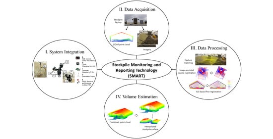
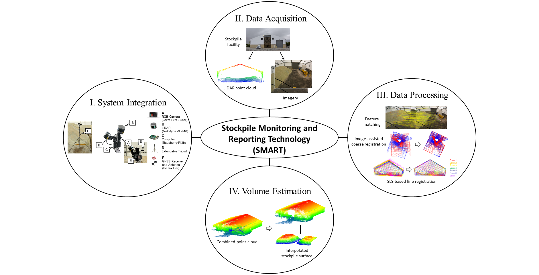
  • Unlike relying on a system-driven approach using sophisticated, expensive encoders and/or inertial measurement units, the SMART system focuses on a data-driven strategy for stockpile volume estimation using only acquired data from a simple, cost-effective acquisition procedure;
  • It is easy to deploy and has the potential of permanent installation in indoor facilities (after suitable modifications of the setup) for continuous monitoring of stockpiles; and,
  • Low-cost, high-precision image/LiDAR hybrid technology such as SMART can influence system manufacturers to develop inexpensive stockpile monitoring solutions, which could be even less expensive.

3. SMART System Integration and Field Surveys

The SMART system is designed to safely and accurately assess stockpile volume. It consists of two LiDAR units (Velodyne VLP-16 Puck) and one RGB camera (GoPro Hero 9) mounted on an extendable tripod (hereafter denoted as a pole). A Raspberry Pi 3b computer, mounted on the same platform, is used to trigger the LiDAR sensors and store their measurement data. The system is also equipped with GNSS and Antenna (U-Blox F9P) that can be used for system georeferencing when operating in outdoor environments. All listed system elements are powered by one energy source, a lithium-polymer battery.

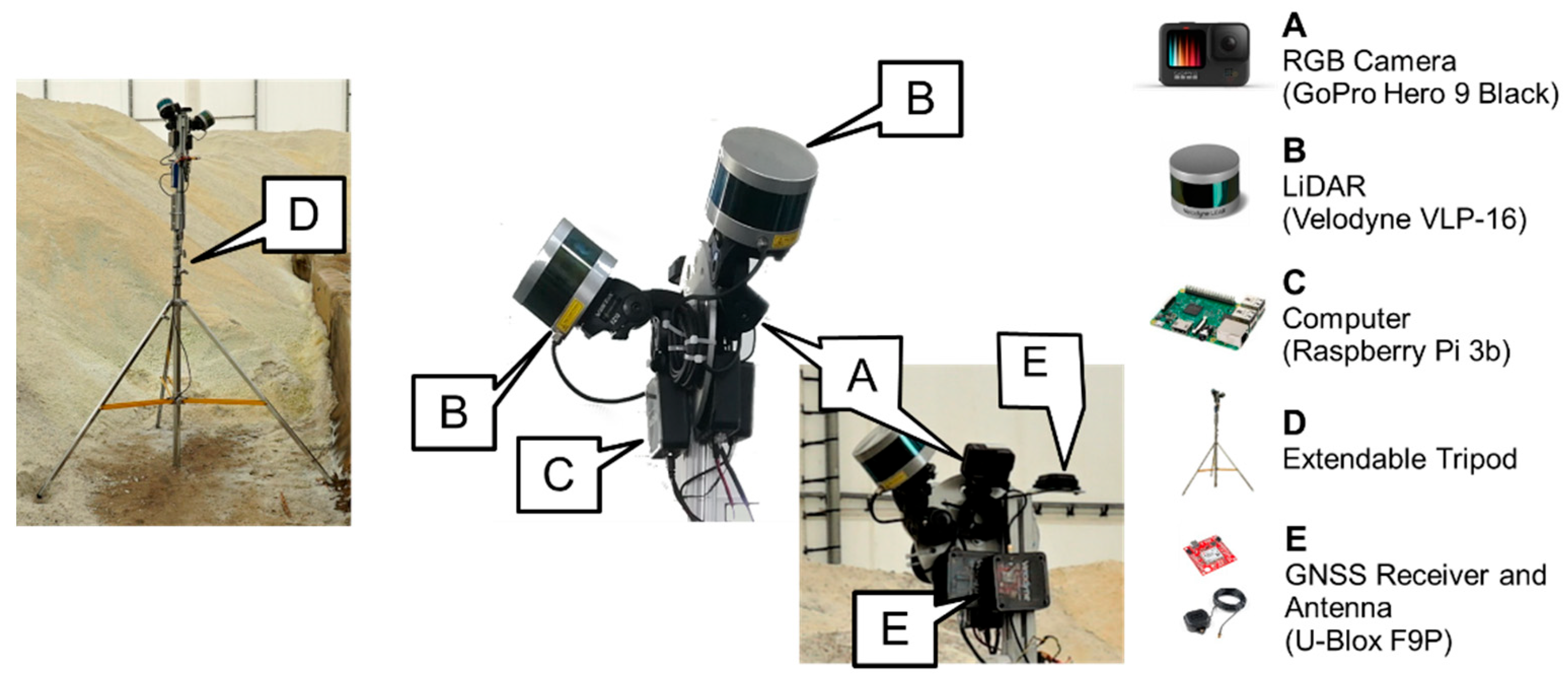
3.1. SMART System Components

The major components of the SMART system are represented in Figure 1. The design of the system (i.e., type, number, and orientation of the sensors) is envisioned to effectively capture indoor facilities. Theoretically, one LiDAR unit can produce enough data for stockpile volume estimation. However, the SMART system is using two LiDAR units to capture data in four directions relative to the system, i.e., left, right, back, and forward, simultaneously, thus reducing the number of required scans. Features (e.g., walls, roof, ground, etc.) captured by the LiDAR sensors are used as a basis to align captured point clouds data with high precision. The RGB camera is included in the system to serve as a tool for the initial (coarse) alignment of the acquired LiDAR data. Additionally, the camera provides a visual record of the stockpile in the storage facility. Through the proposed processing strategy, the utilized sensors will produce well-aligned point cloud with reasonable density (~500 points per square meter at 5 m distance from the system), which can be used as a substitution for more expensive TLS system.
The five major components of the SMART system, i.e., LiDAR units, RGB camera, computer module, system body, and GNSS receiver are described below:
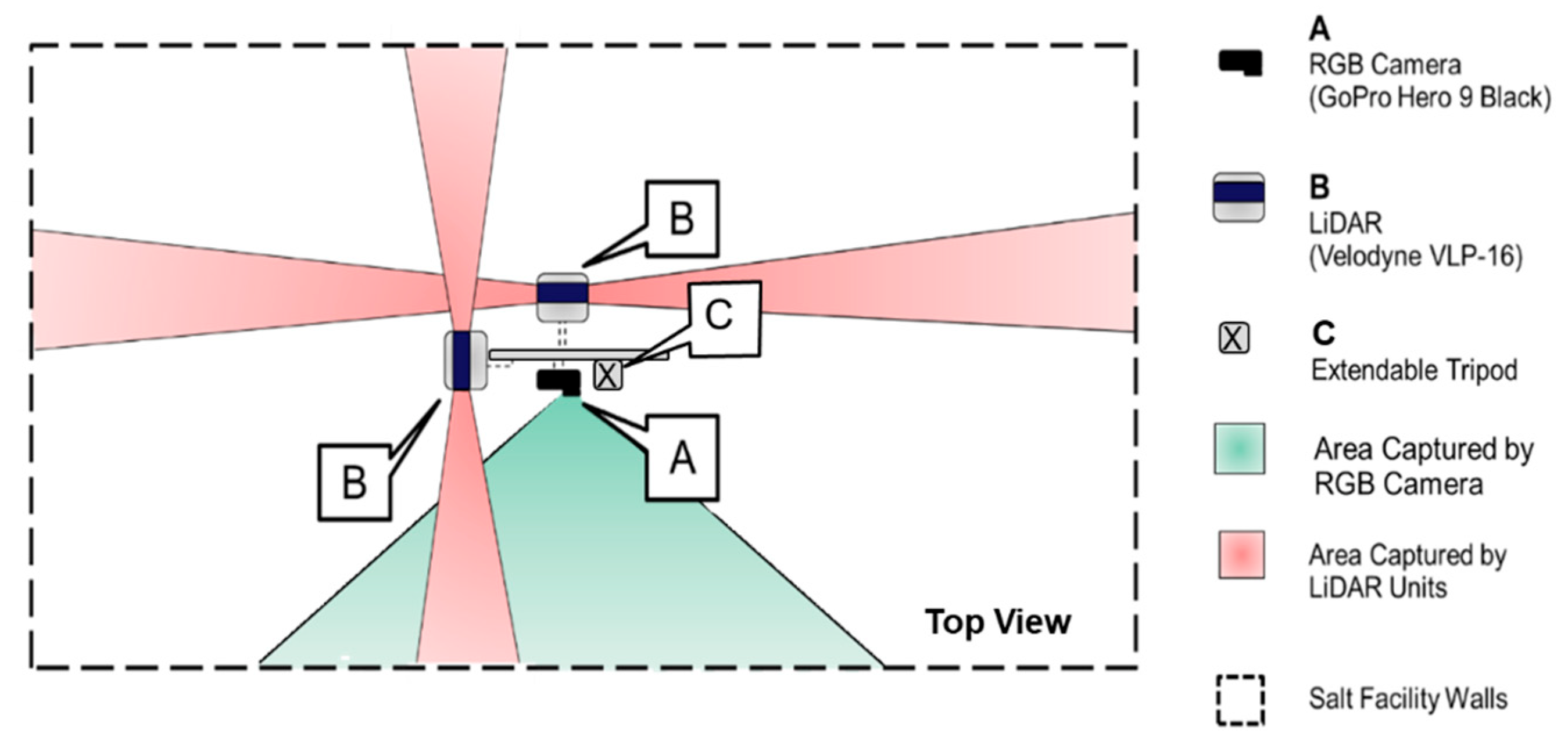
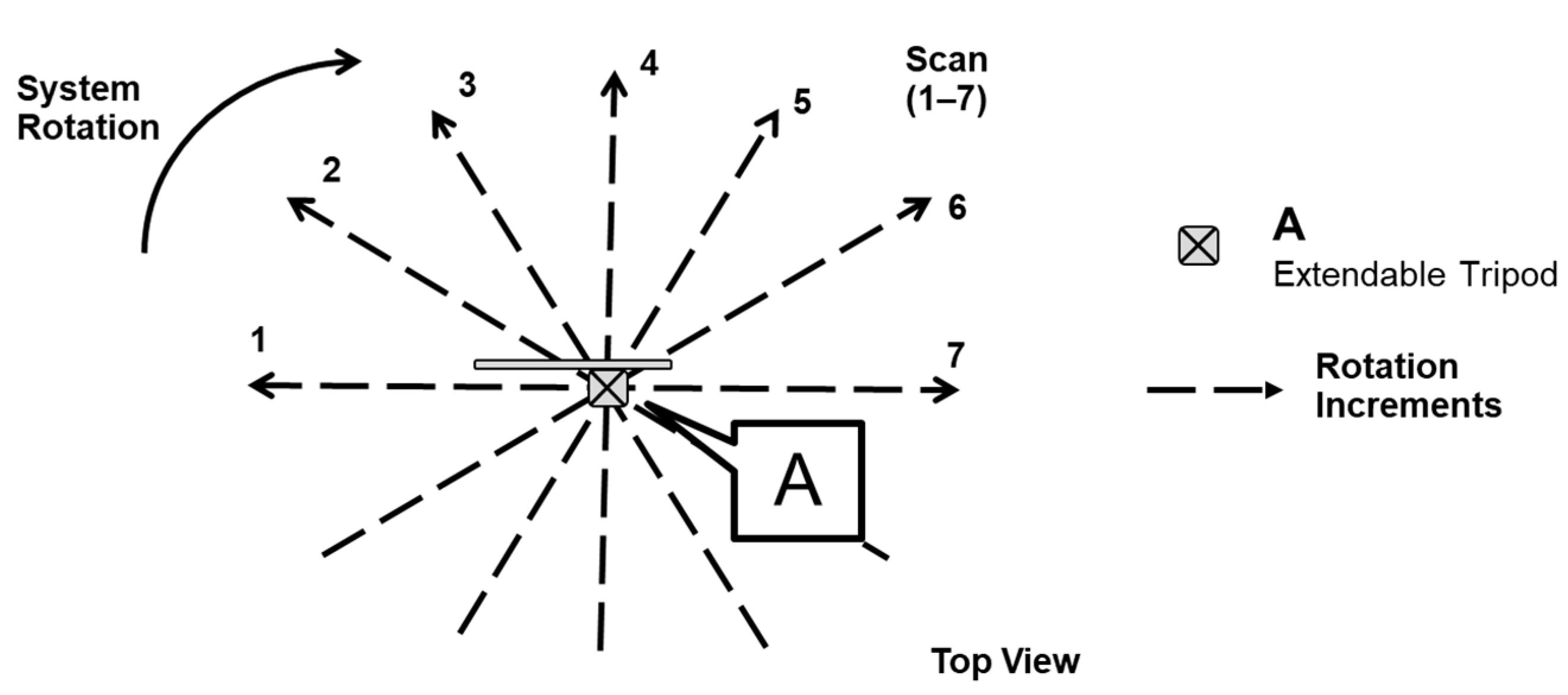
  • LiDAR units: In order to derive a 3D point cloud of the stockpile in question, LiDAR data is first acquired through the VLP-16 sensors. The Velodyne VLP-16 3D LiDAR [48] has a vertical field of view (FOV) of 30° and a 360° horizontal FOV. This FOV is facilitated by the unit construction, which consists of 16 radially oriented laser rangefinders that are aligned vertically from −15° to +15° and designed for 360° internal rotation. The sensor weight is 0.83 kg and the point capture rate in a single return mode is 300,000 points per second. The range accuracy is ±3 cm with a maximum measurement range of 100 m. The vertical angular resolution is 2° and horizontal angular resolution is 0.1–0.4°. The angular resolution of the LiDAR unit enables an average point spacing within one scan line of 3 cm, and between neighboring scan lines of 30 cm at 5 m range (average distance to the salt surface). Given the sensor specifications, two LiDAR units with cross orientation are adopted to increase the area covered by the SMART system in each instance of data collection. The horizontal coverage of the SMART LiDAR units is schematically illustrated in Figure 2. As shown in this figure, two orthogonally installed LiDAR sensors simultaneously scan the environment in four directions. The 360° horizontal FOV of the VLP-16 sensors implies that the entire salt facility within the system’s vertical coverage is captured by the LiDAR units. In addition to the possibility of covering a larger area of the stockpile, this design allows for scanning surrounding structures, thereby increasing the likelihood of acquiring diverse features in all directions from a given scan. These features (linear, planar, or cylindrical) can be used for the alignment of LiDAR data collected from multiple scans to derive point clouds in a single reference frame.
  • RGB camera: The SMART system uses a GoPro Hero 9 camera, which weighs 158 g. The camera has a 5184 × 3888 CMOS array with a 1.4 μ m pixel size and a lens with a nominal focal length of 3 mm. Horizontal FOV of 118° and 69° vertical FOV enable the camera to cover roughly 460 square meters with a 10 m range. A schematic diagram of the camera coverage from the SMART system is depicted in Figure 2. In addition to providing RGB information from the stockpile, images captured by the RGB camera are used to assist the initial alignment process of the LiDAR point clouds collected at a given station. This process will be discussed in detail in Section 4.3.
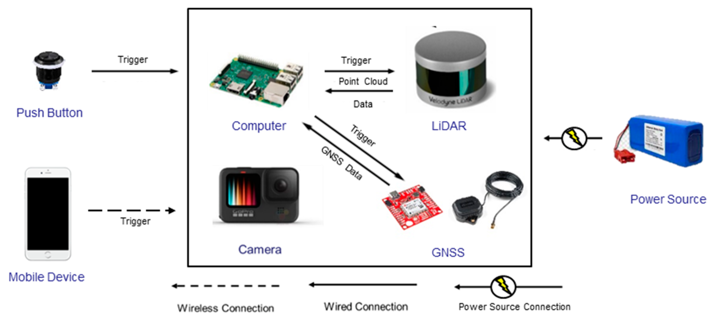
  • Computer module: A Raspberry Pi 3b computer is installed on the system body and is used for LiDAR data acquisition and storage. Both LiDAR sensors are triggered simultaneously through a physical button that has wired connection to the computer module. Once the button is pushed, the Raspberry Pi initiates a 10 s data capture from the two LiDAR units. In the meantime, the RGB camera is controlled wirelessly (using a Wi-Fi connection) through a mobile device, which enables access to the camera’s live view for the operator. All the images captured are transferred to the processing computer through a wireless network. The LiDAR data is transferred from the Raspberry Pi using a USB drive. Figure 3 shows the block diagram of the system indicating triggering signals and communication wires/ports between the onboard sensors and Raspberry Pi module.
  • GNSS receiver and antenna: As one of the potential ways to enhance SMART system capabilities, a GNSS receiver and antenna are added as one of the system components. The purpose of the GNSS unit is to provide location information when operating in outdoor environments. The location information serves as an additional input to aid the point cloud alignment from multiple positions of the system. In this study however, data collection is targeted in a more challenging indoor environment. Therefore, GNSS positioning capabilities of the system are not utilized.
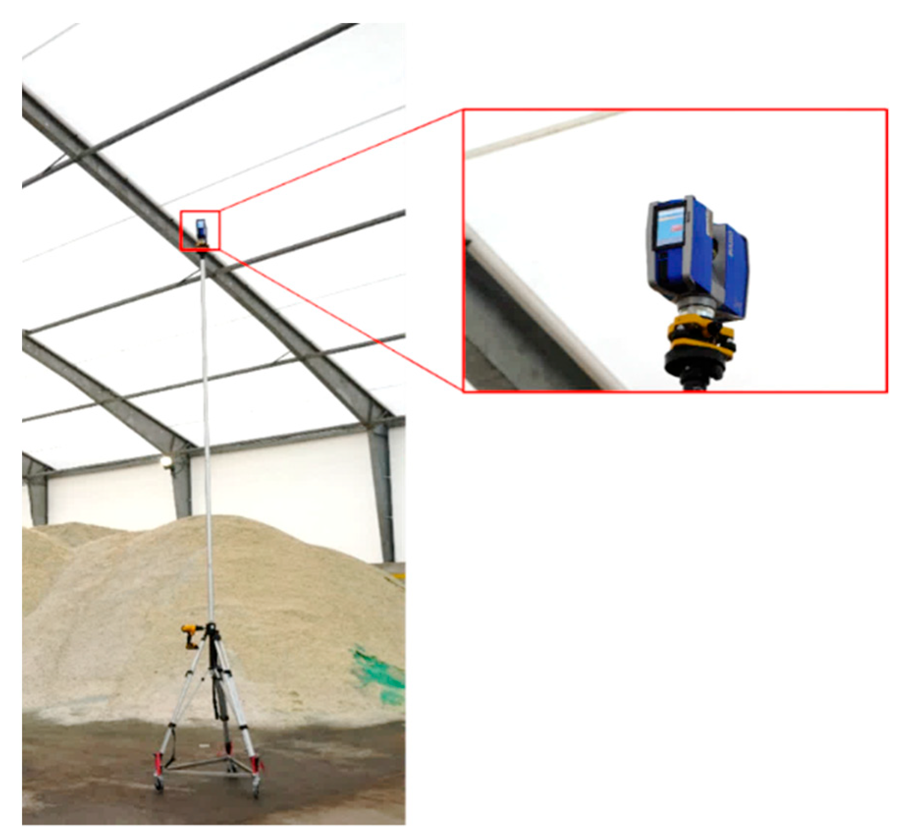
  • System body: LiDAR sensors, an RGB camera, and a GNSS unit of the SMART system are placed on a metal plate attached to an extendable tripod pole that are together considered as the system body. The computer module and power source are located on the tripod pole. The extendable tripod, with a maximum height of 6 m, helps the system minimize occlusions when collecting data from large salt storage facilities and/or stockpiles with complex shapes.

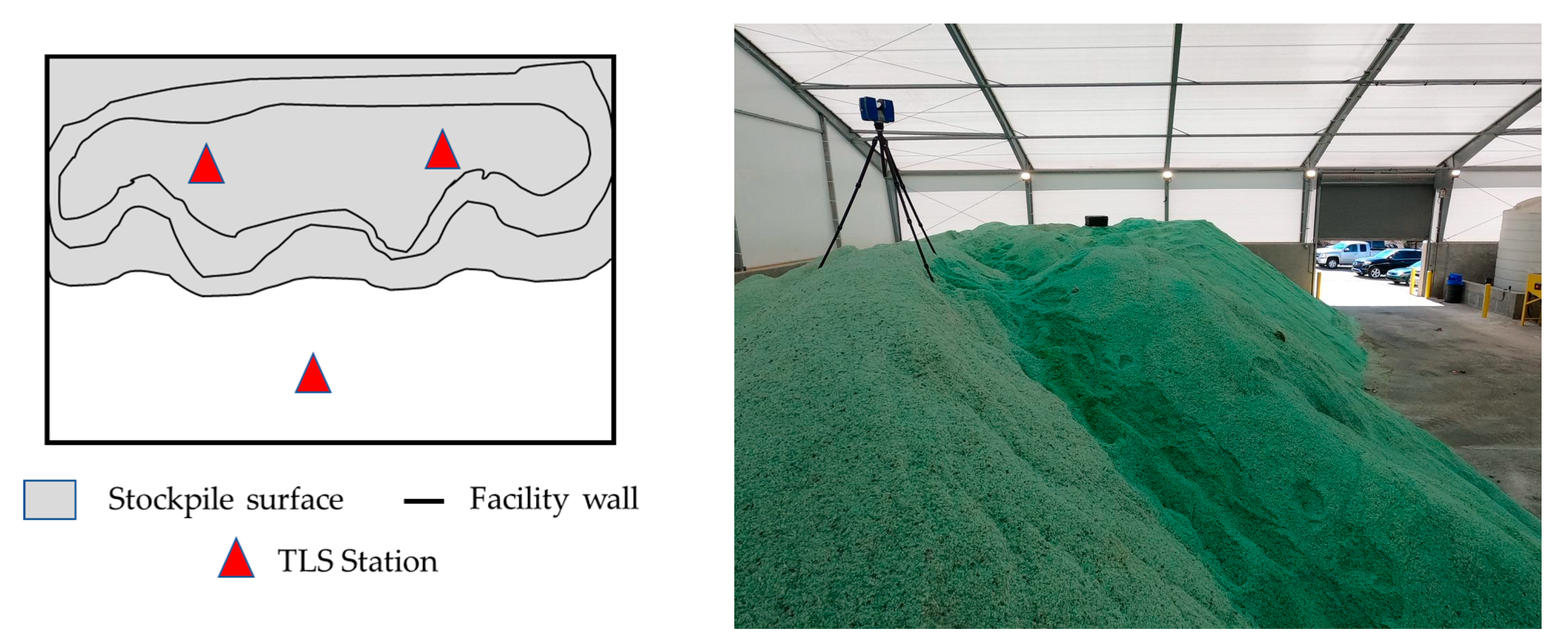
3.2. System Operation and Data Collection Strategy

At each instance of data collection, hereafter referred to as a scan, the SMART system captures a pair of LiDAR point clouds along with one RGB image. With a 30° coverage and orthogonal mounting of LiDAR units, the scan extends to all four sides of the facility. On the other hand, a single RGB image provides only 118° horizontal coverage of the site. In order to obtain complete coverage of the facility, multiple scans from each data collection station are required. To do so, the pole is manually rotated six times around its vertical axis in approximately 30° increments. This process is illustrated in Figure 4. Thus, at a given station, seven LiDAR scans are captured. To ensure that an adequate amount of information is obtained, LiDAR data is captured for 10 s in each scan. The SMART system has a blind spot, i.e., the area under the system, that none of the LiDAR units can capture even after a 180° rotation. The blind spot is common for all tripod-based terrestrial sensors. In many cases, not all stockpile areas can be captured from one station. To solve this issue, data collection is conducted from multiple locations (also referred to as stations). The number of stations varies depending on the shape and size of the stockpile/facility. Having multiple stations also eliminates the previously mentioned blind spot problem.

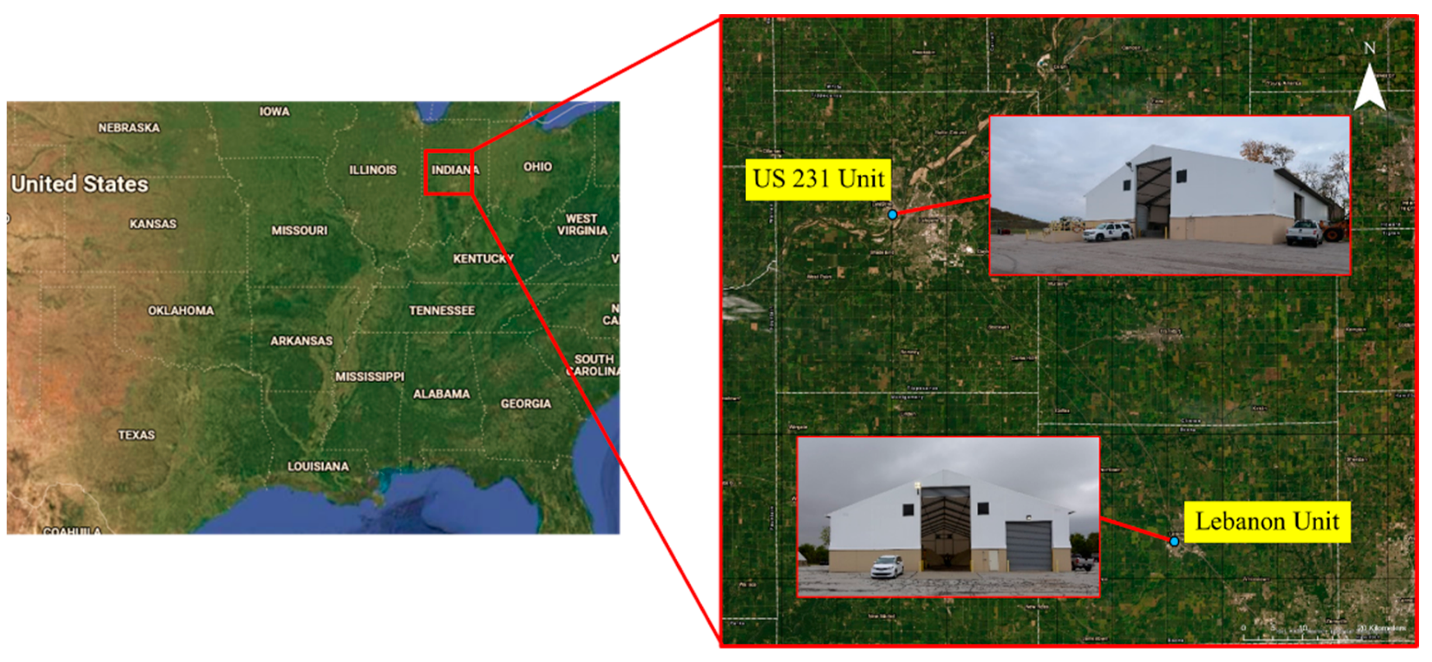
3.3. Dataset Description

In this study, two indoor salt storage facilities with stockpiles of varying size and shape were scanned by the SMART system to illustrate the performance of the developed point cloud registration and volume estimation approaches. These indoor facilities are managed by the Indiana Department of Transportation (INDOT) and used for their winter weather roadway maintenance. Figure 5 shows the location of these facilities. For the purpose of identification, the two datasets are denoted as Lebanon and US-231 units located at Lebanon and West Lafayette, respectively, in Indiana, USA. Finally, to serve as a benchmark for performance evaluation, these storage facilities were also scanned using a terrestrial laser scanner (TLS), FARO Focus, with range accuracy of ±2 mm [18]. The scan resolution for the TLS was set to 12 mm point spacing at 10 m range. The average measurement durations per station for the SMART and TLS were 5 min and 4 min, respectively. Table 2 summarizes the acquired data in the two facilities for this study.

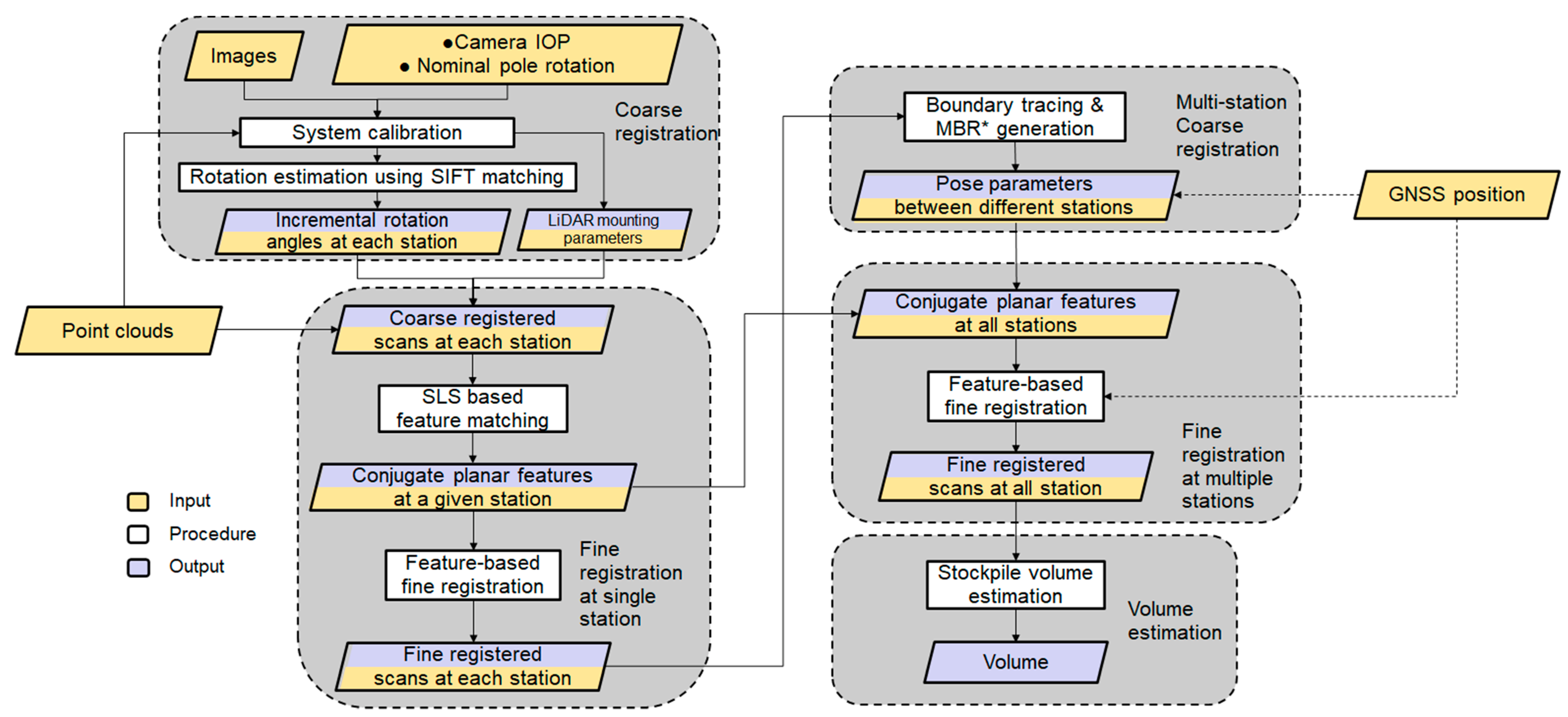
4. Data Processing Workflow

Having introduced the sensors onboard the SMART system and datasets, which will be used for illustrating the processing strategies and conducting the experimental results, the manuscript will now focus on data processing for stockpile volume estimation. The first step involves system calibration to estimate the internal characteristics of the individual sensors as well as the mounting parameters (i.e., lever arm and boresight angles) relating the different sensors. Figure 6 illustrates the workflow of the proposed processing strategy, which is comprised of (1) an image-based coarse registration of captured scans at a given station; (2) feature extraction and fine registration of scans at individual stations; (3) coarse and fine registration of scans from multiple stations; and (4) volume estimation. The image-based coarse registration is introduced to handle the arising challenges from having sparse scans that do not have sufficient overlap. These challenges would not make existing registration strategies applicable. A new segmentation strategy, Scan-Line-based Segmentation (SLS), is introduced to identify planar features, which are used for the fine registration process. Similar to the image-based coarse registration, the SLS is developed to mitigate point cloud sparsity and lack of sufficient overlap among the scans. In this regard, one should note that if the SMART system is used for outdoor stockpile monitoring, the GNSS unit could be utilized to assist both the coarse and fine registration processes. Prior information about pole position from the GNSS can aid the registration by providing an additional constraint for the scan locations, particularly benefiting those with very sparse points. The proposed strategies for coarse and fine registration together with stockpile volume estimation are presented in the following subsections.

4.1. System Calibration

SMART system calibration aims at determining the internal characteristics of the camera and two LiDAR units together with the mounting parameters relating them to the pole coordinate system. The system calibration is based on the mathematical models for image/LiDAR-based 3D reconstruction as represented by Equations (1) and (2). A schematic diagram of the image/LiDAR point positioning equations is illustrated in Figure 7. In these equations, r i c ( k ) represents a vector from the camera perspective center c ( k ) to image point i in the camera frame captured at scan k . This vector is defined as [ x i   x p   d i s t x i y i   y p   d i s t y i c ] T and is derived using the image coordinates of point i and the camera’s principal point coordinates ( x p   and y p   ) , principal distance ( c ), and distortions in the xy-directions for image point i ( d i s t x i and d i s t y i ) .   The scale factor for image point i captured by camera c at scan k is denoted as λ ( i , c , k ) . The position of object point I with respect to the LiDAR unit frame is represented by r I l u j ( k ) and is derived from the raw measurement of LiDAR unit j ( j can be either 1 or 2 for the SMART system), captured at scan k . The position and orientation of the pole frame coordinate system relative to the mapping frame at scan k are denoted as r p ( k ) m and R p ( k ) m . The mounting parameters are defined as follows: r c p and R c p represent the lever-arm and boresight rotation matrix relating the camera system and pole body frame;   r l u j p and R l u j p denote the lever-arm and boresight rotation matrix relating the LiDAR unit j coordinate system and pole body frame. Finally, r I m is the coordinate of object point I in the mapping frame.
r I m = r p ( k ) m + R p ( k ) m r c p + λ ( i , c , k ) R p ( k ) m R c p   r i c ( k )
r I m = r p ( k ) m + R p ( k ) m r l u j p + R p ( k ) m R l u j p r I l u j ( k )
In this study, the internal characteristics parameters (IOP) of the LiDAR units are provided by the manufacturer. To estimate the internal characteristics of the RGB camera (camera IOP), an indoor calibration procedure similar to the one proposed by He and Habib [49] is adopted. More specifically, the camera calibration is conducted using a test field with several checkerboard targets with known distances between the targets. The image coordinates of these targets are manually measured and then used together with the known object distances in a bundle adjustment with system self-calibration procedure. The mounting parameters relating each sensor and the pole coordinate system are derived through a rigorous system calibration procedure similar to the ones developed by Ravi et al. [50] and Zhou et al. [51]. Conceptually, these parameters are derived through an optimization procedure that minimizes discrepancies among conjugate object features (points, linear, planar, and cylindrical) extracted from different LiDAR scans and overlapping images. Since we cannot always assume the availability of information that defines the pole coordinate system relative to the mapping frame (e.g., when using the SMART GNSS unit within an indoor environment), the system calibration cannot simultaneously derive the mounting parameters for the camera and the two LiDAR units. Therefore, the mounting parameters for the first LiDAR unit relative to the pole are not solved for (i.e., they are manually initialized to some reasonable values and treated as constants within the system calibration procedure). To estimate the system calibration parameters, conjugate LiDAR planar features from both units and corresponding image points in overlapping images are manually extracted. The mounting parameters are then estimated by simultaneously minimizing (a) discrepancies among conjugate LiDAR features, (b) back-projection errors of conjugate image points, and (c) normal distance from image-based object points to their corresponding LiDAR planar features.
Once the mounting parameters are estimated, the acquired point clouds from the two LiDAR units for a given scan can be reconstructed with respect to the pole coordinate system. Similarly, the camera position and orientation parameters at the time of exposure (EOP) can also be derived in the same reference frame. As long as the sensors are rigidly mounted relative to each other and the pole, the calibration process need not be repeated.

4.2. Scan Line-Based Segmentation

Having established the LiDAR mounting parameters, planar feature extraction and point cloud coarse registration can be concurrently performed. Planar features from each scan are extracted through a point cloud segmentation process, which takes into consideration the following assumptions/traits of LiDAR scans collected by the SMART system:
(a)
Scans are acquired by spinning multi-beam LiDAR unit(s), i.e., VLP-16;
(b)
LiDAR scans are acquired inside facilities bounded by planar surfaces that are sufficiently distributed in different orientations/locations, e.g., floor, walls, and ceiling;
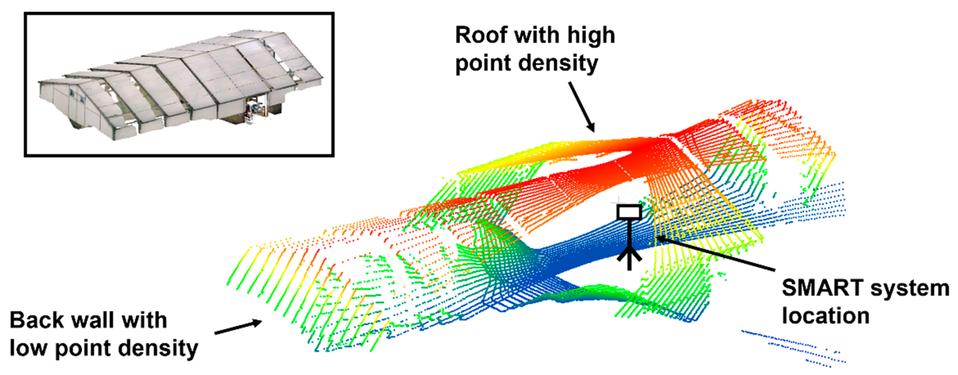
(c)
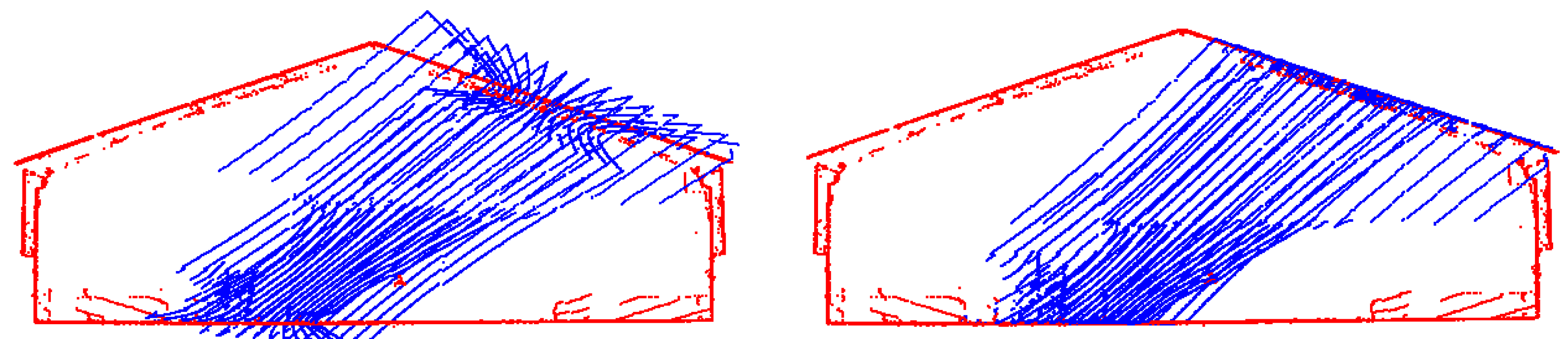
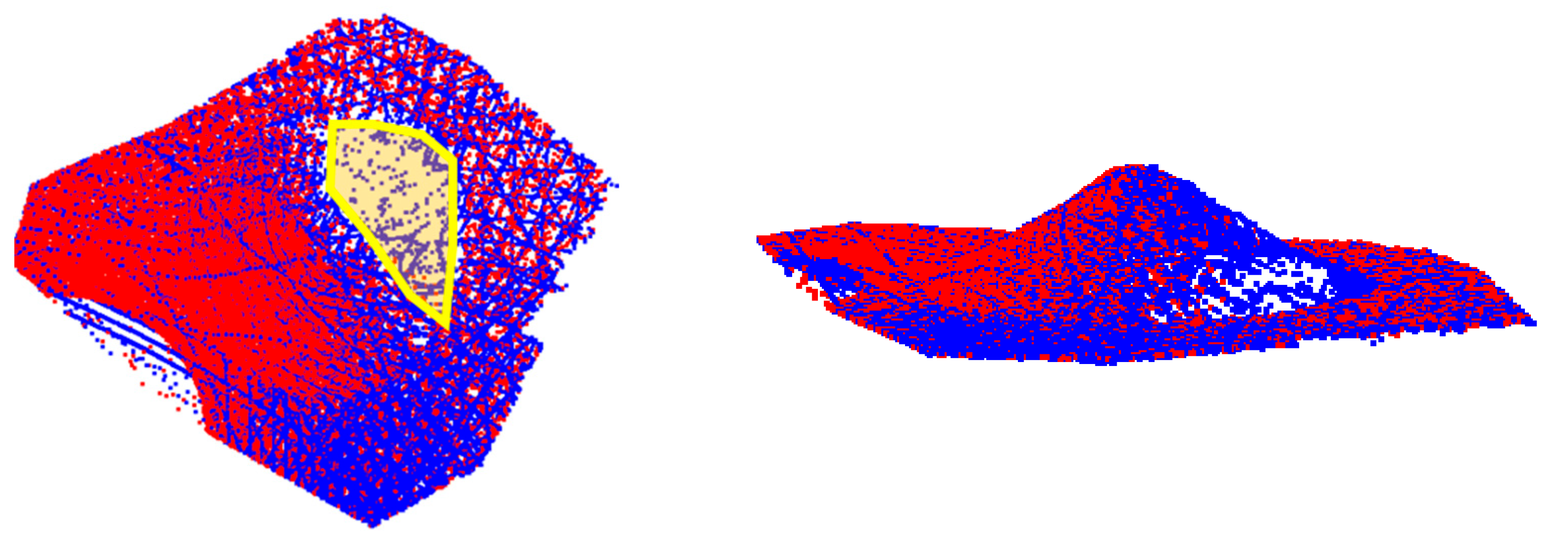
A point cloud exhibits significant variability in point density, as shown in Figure 8.
To consider the above traits/challenges, a scan line-based segmentation (SLS) is proposed. The conceptual basis of SLS is that the locus of a scan from a single beam will trace a smooth curve as long as the beam is scanning successive points belonging to a smooth surface (such as planar walls, floor, or roofs). Therefore, the developed strategy starts by identifying smooth curve segments (for each laser beam scan). Combinations of these smooth curve segments are used to identify planar features. A smooth curve segment is assumed to be composed of a sequence of small line segments that exhibit minor change in orientation between neighboring line segments. To identify these smooth curve segments, starting from a given point p i along a laser beam scan, two consecutive sets of sequentially scanned points, i.e., S i = { p i ,   ,   p i + n 1 } and S i + 1 = { p i + 1 ,   ,   p i + n } , are first inspected. The criteria for identifying whether a given set, S i + 1 , is part of a smooth curve segment defined by S i , are (1) the majority of points within the set S i + 1 can be modeled by a 3D line, which is derived through an iterative least-squares adjustment with outlier removal process (i.e., the number of outliers should be smaller than a threshold n T ); (2) the orientation of the established linear feature is not significantly different from that defined by the previous set S i (i.e., the angular difference should be smaller than a threshold α T ). Whenever the first criterion is not met, a new smooth segment is initiated starting with the next set. On the other hand, when the second criterion is not met, a new smooth segment is initiated starting with the current set. One should note that the moved set is always shifted one point at a time. In addition, a point could be classified as pertaining to more than one smooth segment.
To ensure that the derived smooth curve segments are not affected by the starting point location, the process terminates with a cyclic investigation of continuity with the last scanned points appended by the first n points. A detailed demonstration of the SLS approach for a single laser beam is provided in Figure 9. In this paper, the parameter n, used to define a set of points pertaining to the small line segments, is selected as 20. This value is based on the point density along each scan line to ensure a reasonable length of the line segments. Similarly, the outlier percentage threshold is selected as 20% according to the noise level in the LiDAR data. An example of the original point cloud for a given laser beam scan and its derived smooth curve segments is shown in Figure 10a,b. For a calibrated system, the piece-wise smooth curve segmentation is performed for derived point clouds from the two LiDAR units at a given scan, wherein each laser beam from each unit is independently segmented. Figure 10c shows the derived smooth curve segments for one scan captured by the two LiDAR units.
The next step in the SLS workflow is to group smooth curve segments that belong to planar surfaces. This is conducted using a RANSAC-like strategy. For a point cloud (a LiDAR scan in this study) that is comprised of a total of n s smooth curve segments, a total of C n s 2 pairings are established. Among all pairings, only the ones originating from different laser beams are investigated. For each of these pairings, an iterative least squares-based plane fitting with built-in outlier removal is conducted. The iterative plane fitting starts with the points from a pair of curve segments as initial inliers. The process keeps finding new inliers and updates the plane parameters until the number of inliers does not change significantly between iterations. Then, all remaining smooth curve segments are checked to evaluate whether the majority of the points belong to the plane defined by the pair of curve segments in question. This process is repeated for all the pairs to obtain possible planar surfaces (along with their constituent smooth curve segments). The planar surface with the maximum number of points is identified as a valid feature and its constituent curve segments are dropped from the remaining possible planar surfaces. Then, the process of identifying the best planar surface amongst the remaining curve segments is repeated until no more planes can be added. The difference between the proposed segmentation strategy and RANSAC is that we perform an exhaustive investigation of all possible curve segment pairings to ensure that we get as complete planar segments as possible. This is critical given the sparse nature of the scan. Figure 10d illustrates the results of planar feature segmentation for the scan shown in Figure 10c.

4.3. Image-Based Coarse Registration

In this step, the goal is to coarsely align the LiDAR scans at each station. At the conclusion of this step, LiDAR point clouds from S scans (e.g., S = 7 ) at a given station are reconstructed in a coordinate system defined by the pole at the first scan. In other words, the pole coordinate system at the first scan ( k = 1 ) is considered as the mapping frame, i.e., r p ( 1 ) m is set to [ 0 0 0 ] T and R p ( 1 ) m is set as an identity matrix. For the SMART system, we assume that the pole does not translate between scans at a given station, i.e., r p ( k ) m = r p ( 1 ) m , but is incrementally rotated with a nominal rotation around the pole Z axis (−30° in the suggested set-up). One should note that, although there might be small translation between different scans, assuming a constant position of the pole after its rotation is a reasonable assumption for conducting a coarse registration of point clouds at a given station. Therefore, considering the point positioning equation, Equation (2), and given the system calibration parameters r l u j p and R l u j p , the coarse registration problem now reduces to the estimation of pole rotation matrices R p ( k ) p ( 1 ) , with k ranging from 2 to 7.
The rotation matrices R p ( k ) p ( 1 ) can be derived through the incremental pole rotation estimates between successive scans, i.e., R p ( k ) p ( k 1 ) ( 2 k 7 ). One should note that, although the incremental rotation matrix is nominally known based on the SMART data collection strategy, e.g., the rotation R p ( k ) p ( k 1 ) can be assumed to be Rx(0°)Ry(0°)Rz(−30°), such rotation might not lead to point clouds with reasonable alignment. Figure 11 shows an example of the combined point clouds from the two LiDAR units collected at two scans ( k = 3 and k = 5 ) for the single station in the US-231 dataset while using the nominal rotation angles for coarse registration. As can be seen in this figure, there is a significant misalignment between reconstructed point clouds.
Due to the featureless nature of stockpile surfaces, sparsity of individual LiDAR scans, and insufficient overlap between successive scans, establishing conjugate features for coarse registration of multiple scans is a challenging task. To overcome this limitation, an image-aided LiDAR coarse registration strategy is proposed. More specifically, we first derive the incremental camera rotation angles using a set of conjugate points established between successive images. Then, the pole rotation angles are derived using the estimated camera rotations and system calibration parameters. Due to the very short baseline between images captured at a single station, conventional approaches for establishing the relative orientation using essential matrix and epipolar geometry, e.g., the Nister approach [52], are not applicable. Therefore, the incremental rotation between successive scans is estimated using a set of identified conjugate points in the respective images while assuming that the camera is rotating around its perspective center. The remainder of this section addresses the estimation of the incremental camera rotation using a set of conjugate points and then proceeds by introducing the proposed approach for the identification of these conjugate points.
For an established conjugate point between images captured at scans k 1 and k from a given station, Equation (1) can be reformulated as Equation (3), which can be further simplified to the form in Equation (4). Assuming that the components of camera-to-pole lever arm r c p are relatively small, { R p ( k 1 ) 1 R p ( k ) 1 }   r c p can be expected to be close to 0. Given the pole-to-camera boresight matrix R p c , the incremental camera rotation R c ( k ) c ( k 1 ) can be represented as R p c   R p ( k ) p ( k 1 )   R c p . Therefore, Equation (4) can be reformulated to the form in Equation (5). Given a set of conjugate points, the incremental camera rotation matrix R c ( k ) c ( k 1 ) can be determined through a least squares adjustment to minimize the sum of squared differences i = 1 m [ r i c ( k 1 ) λ ( i , c , k 1 , k )   R c ( k ) c ( k 1 )   r i c ( k ) ] 2 , where m is the number of identified conjugate points in the stereo-pair in question. To eliminate the scale factor λ ( i , c , k 1 , k ) from the minimization process, the vectors r i c ( k 1 ) and r i c ( k ) can be reduced to their respective unit vectors, i.e., r ¯ i c ( k 1 ) and r ¯ i c ( k ) . Thus, R c ( k ) c ( k 1 ) can be determined by minimizing i = 1 m [ r ¯ i c ( k 1 )   R c ( k ) c ( k 1 )   r ¯ i c ( k ) ] 2 . Estimation of R c ( k ) c ( k 1 ) can be realized through a closed-form solution using quaternions by identifying the eigenvector corresponding to the largest eigenvalue for a ( 4 × 4 ) matrix defined by the pure quaternion representations of r ¯ i c ( k 1 ) and r ¯ i c ( k ) [53]. One should note that estimating the incremental camera rotation angles requires a minimum of three well-distributed, conjugate points in two successive images. Once the incremental camera rotation matrices are derived, the rotation between the camera at a given scan k and the camera at the first scan can be estimated through rotation matrix concatenation, i.e., R c ( k ) c ( 1 )   = R c ( 2 ) c ( 1 ) R c ( 3 ) c ( 2 ) R c ( k ) c ( k 1 ) . Finally, the pole rotation between scan k and the first scan can be derived, i.e., R p ( k ) p ( 1 ) can be defined as   R c p R c ( k ) c ( 1 ) R p c . Now, the coarse registration of different pole scans at a given location reduces to the identification of a set of conjugate points between successive images.
r I m ( k 1 ) = R p ( k 1 ) p ( 1 ) r c p + λ ( i , c , k 1 ) R p ( k 1 ) p ( 1 ) R c p   r i c ( k 1 ) r I m ( k ) = R p ( k ) p ( 1 ) r c p + λ ( i , c , k ) R p ( k ) p ( 1 ) R c p   r i c ( k )     }
{ R p ( k 1 ) p ( 1 ) R p ( k ) p ( 1 ) } r c p + λ ( i , c , k 1 ) R p ( k 1 ) p ( 1 ) R c p   r i c ( k 1 ) = λ ( i , c , k ) R p ( k ) p ( 1 ) R c p   r i c ( k )
r i c ( k 1 ) = λ ( i , c , k 1 , k )   R c ( k ) c ( k 1 )   r i c ( k )
Due to the featureless nature of the stockpile surface as well as the presence of repetitive patterns inside a storage facility (e.g., beam junctions, bolts, window corners, etc.) as well as the inability to use epipolar constraints for images with a short baseline, traditional matching techniques would produce a large percentage of outliers. Therefore, we propose a rotation-constrained image matching strategy where the nominal pole rotation can be used to predict the location of a conjugate point in an image for a selected point in another one. In this regard, one can use Equation (5) to predict the location of a point in image k 1 for a selected feature in image k . To simplify the prediction process, the unknown scale factor λ ( i , c , k 1 , k ) can be eliminated by dividing the first and second rows by the third one, resulting in Equation (6), where x i ' and y i ' are the image coordinates of conjugate points after correcting for the principal point offsets and lens distortions. The remainder of this subsection discusses the proposed image matching strategy, referred to as rotation-constrained image matching, by first discussing the limitations of traditional matching algorithms when it comes to finding conjugate features in images captured in stockpile facilities.
x i ' c ( k 1 ) = c r 11   x i ' c ( k ) + r 12   y i ' c ( k ) r 13   c r 31   x i ' c ( k ) + r 32   y i ' c ( k ) r 23   c y i ' c ( k 1 ) = c r 21   x i ' c ( k ) + r 22   y i ' c ( k ) r 23   c r 31   x i ' c ( k ) + r 32   y i ' c ( k ) r 23   c     }
Rotation-constrained image matching: Commonly used image matching strategies are based on a detect-and-describe framework where first a set of interest points are detected in an image pair and then a descriptor is generated for each detected feature using a local region around that feature. Various feature detector and descriptor approaches such as SIFT [39] have been developed and thoroughly evaluated [54,55,56]. For detected features in a stereo pair, denoted hereafter as left and right images, traditional approaches establish conjugate points through comparison of each feature descriptor in the left image with all feature descriptors in the right image (i.e., exhaustive search is conducted) as can be seen in Figure 12. Exhaustive search performs well for images with distinct point features. However, in images with repetitive patterns, which is a key characteristic of stockpile images, there will be a very high similarity between the feature descriptors, thus resulting in a high percentage of outliers as can be seen in Figure 13 for a stereo-pair in the US-231 dataset.
In this study, nominal rotation angles between images are used in an iterative procedure to reduce the matching search space and thus mitigate matching ambiguity. Figure 14 shows the workflow of the proposed rotation-constrained image matching approach. In the first step, the SIFT detector and descriptor algorithm is applied on all images captured at a single station. Then, lens distortions are removed from the coordinates of detected features. Next, two successive images are selected for conducting image matching. In the fourth step, the incremental rotation matrix of the camera for the selected successive scans is initially defined using the nominal pole rotation angles while considering the camera mounting parameters. Given the nominal rotation matrix and extracted features, in the next step, an iterative procedure (Steps 5 and 6) is adopted to establish conjugate features and consequently, refine the incremental camera rotation angles between the two images.
In the iterative procedure, each extracted feature in the left image is projected to the right image using the current estimate of incremental camera rotation angles: Equation (6). The predicted point in the right image is then used to establish a search window with a pre-defined dimension. This process is shown in Figure 15a. The search window size is determined according to the reliability of the current estimate of pole rotation angles as well as camera system calibration parameters. Accordingly, in our experiments, a window size of 1000 × 1000 pixels is selected for the first iteration. Among all SIFT features in the right image, only those located inside the search window are considered as potential conjugate features. This strategy could eliminate some of the matching ambiguities caused by repetitive patterns in the imagery. Once a feature in the right image is selected as a matching hypothesis, a left-to-right and right-to-left consistency check is conducted to remove more matching outliers. In the sixth step, conjugate features are used to refine the incremental camera rotation between the two successive scans using the abovementioned quaternion-based least squares adjustment. At this stage, established conjugate points in the left image are projected to the right one using the refined rotation angles, and the root-mean-square error (RMSE) value of coordinate differences between the projected points and their corresponding features in the right image is estimated. The RMSE value is referred to as projection residual. Steps 5 and 6 are repeated until the projection residual is smaller than a threshold (e.g., 40 pixels) or a maximum number of iterations (e.g., 5) is reached. Considering the camera to object-space distance in our experiments, it is expected that the estimated pole rotation matrix with ~40 pixels projection error leads to a reasonable coarse registration. Additionally, the maximum number of iterations is selected as five to establish a trade-off between the processing efficiency and alignment quality among point clouds after the coarse registration.
One should note that, with the progression of iterations, more reliable conjugate features are established, and therefore, the estimated incremental rotation angles between successive images become more accurate. Consequently, the search window size is reduced by a constant factor after each iteration to further reduce matching ambiguity. A conservative reduction factor of 0.8 is selected in our experiments to strike a balance between efficiency and reliability against missing correct correspondences. This process is schematically shown in Figure 15b. Figure 16 shows sample matching results from the rotation-constrained matching strategy after one iteration (Figure 16a) and two iterations (Figure 16b) for the stereo-pair illustrated in Figure 13. Comparing Figure 13 and Figure 16, one can observe an improvement in the quality of matches, i.e., decrease in the percentage of outliers, when using the rotation-constrained matching. Additionally, through closer inspection of Figure 16a,b, we can see an increase in the number of matches, improvement in distribution of conjugate points, and decrease in the projection residual in the iterative approach compared to the case when relying on nominal rotation angles only, i.e., rotation-constrained matching with one iteration. To illustrate the feasibility of the proposed matching strategy, Figure 17 shows the post-coarse registration alignment for the scans in Figure 11, which had been originally aligned using the nominal pole incremental rotation.

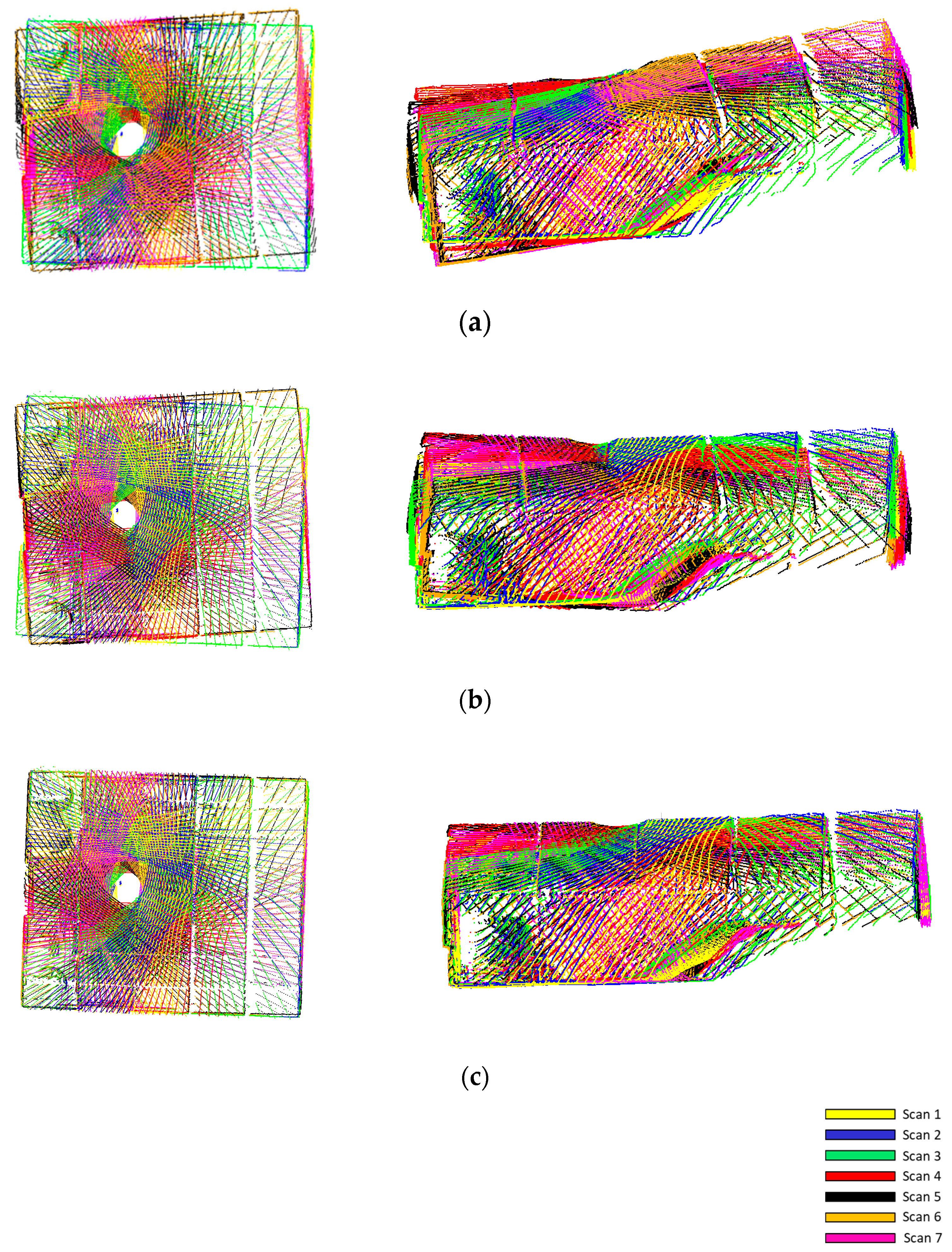
4.4. Feature Matching and Fine Registration of Point Clouds from a Single Station

Once the LiDAR scans are coarsely aligned, conjugate planar features in these scans are identified through the similarity of surface orientation and spatial proximity. In other words, segmented planar patches from different scans are first investigated to identify planar feature pairs that are almost coplanar. A planar feature pair is deemed coplanar if it fulfills two criteria–first, the angle between their surface normals does not exceed a threshold angle. Given reasonable alignment of point clouds after coarse registration, this threshold is assigned a small value, e.g., 3°. Second, the plane-fitting RMSE of the merged planes R M S E T   is not significantly larger than the plane-fitting RMSE for the individual planes R M S E p 1 ,   R M S E p 2 ; i.e., R M S E T = n R M S E × max ( R M S E p 1 ,   R M S E p 2 ) , where n R M S E is a user-define multiplication factor. Once the coplanarity of a planar feature pair is confirmed, the spatial proximity of its constituents is checked in order to reject matches between two far planes. An accepted match is considered as a new plane and the process is repeated until no additional planes can be matched.
Following the identification of conjugate planes, a feature-based fine registration is implemented, as described by Lin et al. [57]. The key characteristic of the adopted fine registration strategy is simultaneous alignment of multiple scans using features that have been automatically identified in the point clouds. Moreover, the post-alignment parametric model of the registration primitives is also estimated. In this study, identified planar features extracting along the floor, walls, and ceiling of the facility are used as registration primitives. The conceptual basis of the fine registration is that conjugate features would fit a single parametric model after registration. The unknowns of the fine registration include the transformation parameters for all the scans except one (i.e., one of the scans is used to define the datum for the final point cloud) as well as the parameters of the best fitting planes. In terms of the parametric model, a 3D plane is defined by the normal vector to the plane and signed a normal distance from the origin to the plane. The fine registration parameters are estimated through a least-squares adjustment by minimizing the squared sum of normal distances between the individual points along conjugate planar features and best fitting plane through these points following the point cloud alignment.
A transformed point in the mapping frame, r I m , can be expressed symbolically by Equation (7), where r I k is an object point I in scan k; t k m denotes the transformation parameters from scan k to the mapping frame as defined by the reference scan. The minimization function is expressed mathematically in Equation (8), where f b m denotes the feature parameters for the b t h . feature; n d ( r I m ,   f b m ) denotes the post-registration normal distance of the object point from its corresponding feature. Figure 18 presents the conceptual basis of the fine registration together with sample point clouds before and after feature-based fine registration, where the improvement in alignment can be clearly seen. The root mean square of the normal distances between the aligned point cloud for all the features and their respective fitted planes is adopted as a quality control metric. For truly planar features, the RMSE should be a fraction of the ranging noise for the used LiDAR units. In other words, the RMSE of the normal distances from the best fitting plane is expected to be within the bounds defined by the ranging noise. To consider situations where the used primitives are not perfectly planar, the RMSE is expected to be two to three times the range noise.
r I m = f ( t k m ,   r I k )
argmin t k m , f b m   scans   and   features n d 2 ( r I m ,   f b m )

4.5. Coarse Registration of Point Clouds from Multiple Stations

At this stage, point clouds from the same station are well-aligned. The goal of this step is to coarsely align point clouds from different stations, if available. Assuming that the planimetric boundary of the involved facility can be represented by a rectangle, the multi-station coarse registration can be conducted by aligning these rectangles. The process starts with levelling and shifting the registered point clouds from each station until the ground of the facility aligns with the XY plane. Then, the point clouds are projected onto the XY plane and the outside boundaries are traced using the approach proposed by Sampath [58] (see Figure 19a). Next, the minimum bounding rectangle (MBR) [59] of the boundary for each station is derived: each MBR is represented by four points, as shown in Figure 19b. Finally, the inter-station coarse registration is realized by aligning the four points representing the MBRs from the different stations. In the SMART operation, the pole orientation in the first scan at each station is set up to have a similar orientation relative to the facility. Since the pole coordinate system at the first scan for different stations is used as a reference, the coarse registration rotation angles in the XY-plane should be small (i.e., there will be no ambiguity in rotation estimation for multi-station coarse registration when dealing with rectangular facilities). Following the multi-station coarse registration, a feature matching and fine registration step similar to what has been explained in Section 4.4 for single station is repeated while considering all the scans at all the stations.

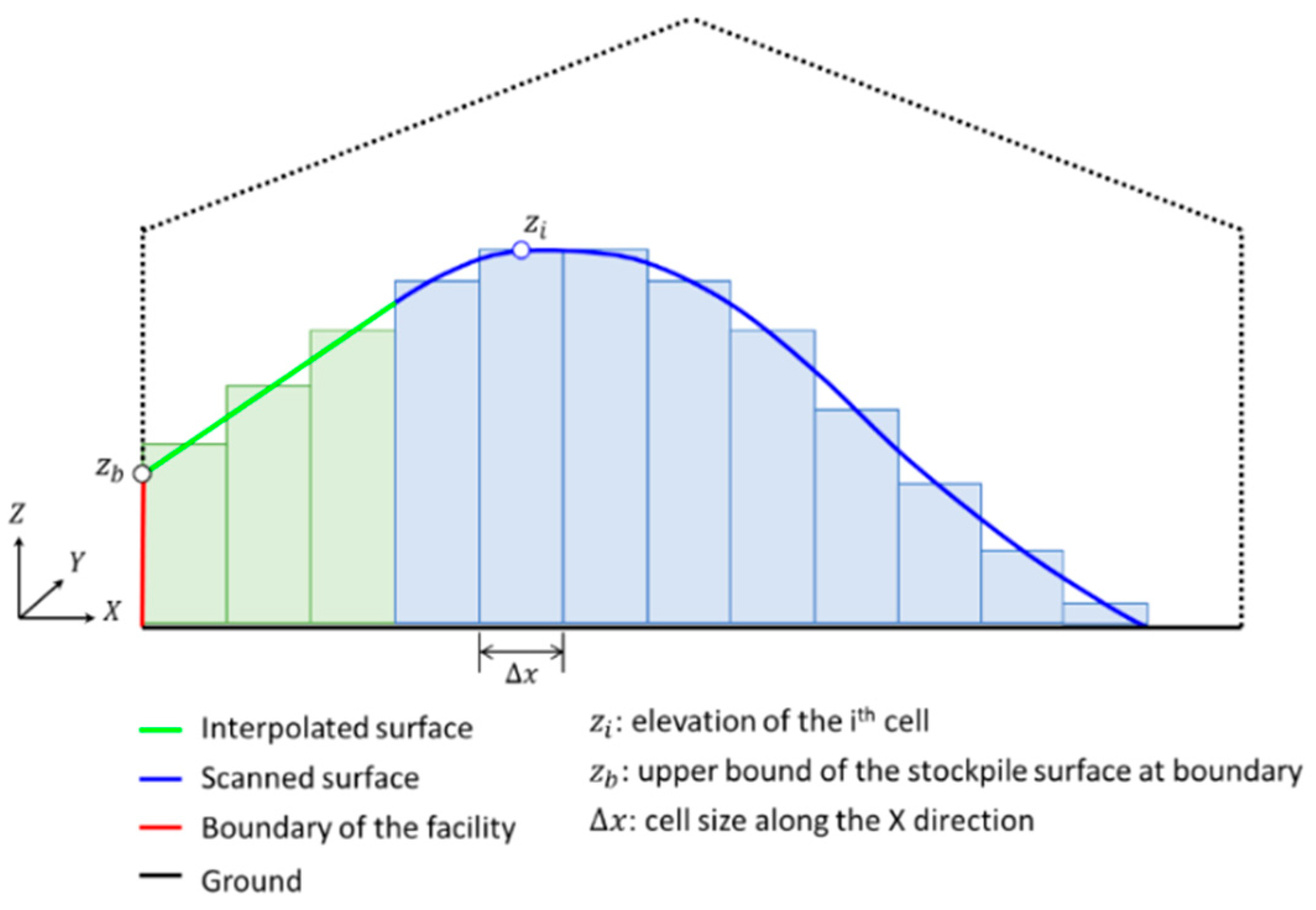
4.6. Volume Estimation

For volume estimation, a digital surface model (DSM) is generated using the levelled point cloud for the scanned stockpile surface and boundaries of the facility. To generate the DSM, first, grid cells of identical size are defined in the XY plane over the stockpile area. The cell size is chosen based on a rough estimate of the average point spacing (0.1 × 0.1 m in this research). Then, each cell is assigned a height based on an interpolated elevation of the stockpile surface at the center of the cell. A Delaunay triangulation-based bilinear interpolation is implemented for this purpose. It is reasonable to assume that occlusions will occur regardless of the system setup in the facility. The interpolation, therefore, enables the derivation of stockpile surface in occluded areas, particularly between the scanned surface and facility boundaries. Finally, the volume (V) is defined according to Equation (9), where n c e l l is the number of DSM cells, z i is the elevation at the ith DSM cell, z g r o u n d is the elevation of ground, and Δ x and Δ y are the cell size along the X and Y directions, respectively. Figure 20 shows a 2D schematic diagram that illustrates the 3D volume estimation process. The space bounded by the scanned surface (blue line), ground (black line), boundary of the facility (red line), and interpolated surface (green line) would be the estimated stockpile volume.
V = i = 1 n c e l l ( z i z g r o u n d ) Δ x Δ y

5. Experimental Results and Discussion

This section evaluates the capability of the developed SMART system for stockpile volume estimation using the datasets introduced earlier. Before reporting the volume estimation results, we first list the system calibration results and then evaluate the performance of the developed strategies for coarse and fine registration of the point clouds collected by the SMART system. C++ programming was used for the development of an in-house implementation of the coarse and fine registration strategies. For the image-based coarse registration, OpenCV [60] implementation of SIFT was used as the feature detector and descriptor algorithm.

5.1. System Calibration Results

In this study, a system calibration dataset was collected inside a high-bay facility located at the Agronomy Center for Research and Education (ACRE) in Purdue University. Figure 21 shows sample images of the calibration site. The images show the presence of sufficient number of planar features (e.g., ground, walls, ducts, table surfaces, and gates), which would facilitate the SMART system calibration.
The estimated system calibration parameters along with their standard deviations are presented in Table 3. As mentioned in Section 4.1, the mounting parameters between the first LiDAR unit and pole coordinate system are fixed (shown in red in Table 3). Given the standard deviation (Std. Dev.) values, one can conclude that the estimated mounting parameters are precise. With the mounting parameters known, point clouds from the two LiDAR units at a given scan can now be registered to the pole coordinate frame. Figure 22 shows point clouds from the two LiDAR units at a given scan before and after calibration.

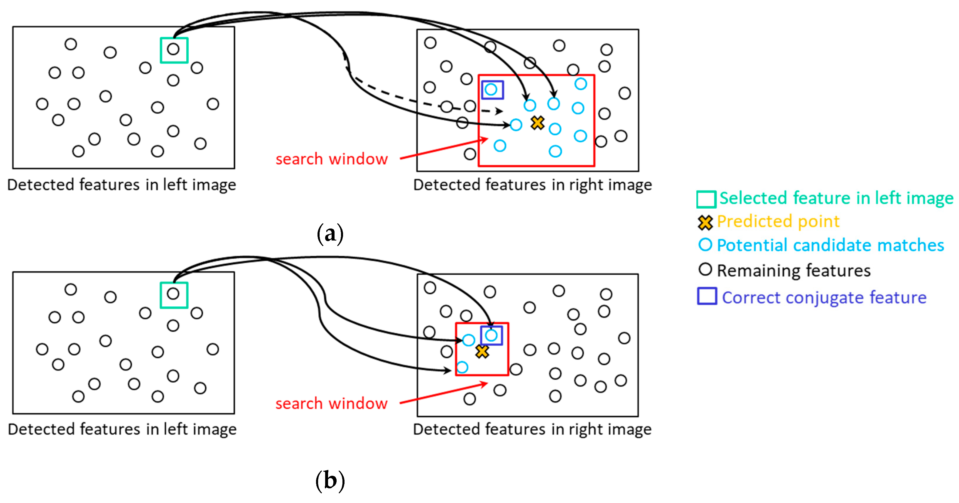
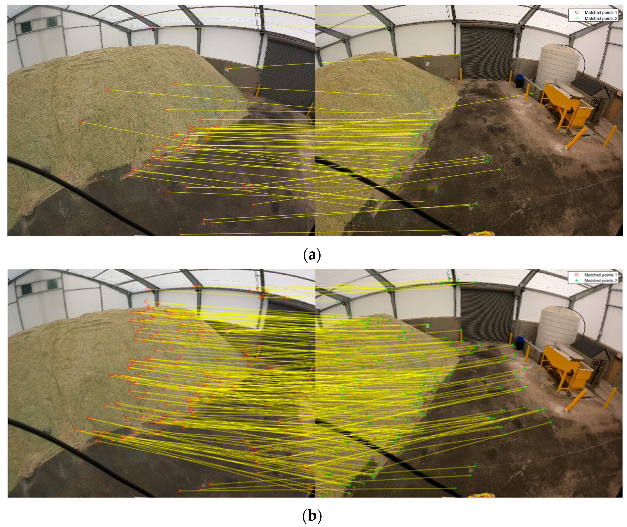
5.2. Results of Image-Based Coarse Registration at a Single Station

In this subsection, the performance of the proposed feature matching algorithm for image-based coarse registration is evaluated. The feasibility of the constrained image matching is verified by comparing the estimated incremental rotation angles against those derived from traditional exhaustive image matching and manually established conjugate points. More specifically, the following criteria are used for this evaluation:
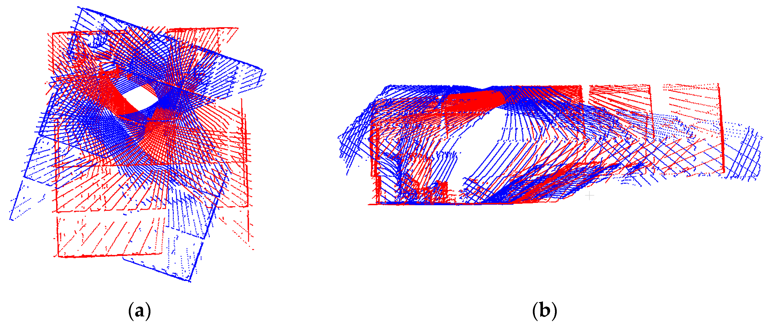
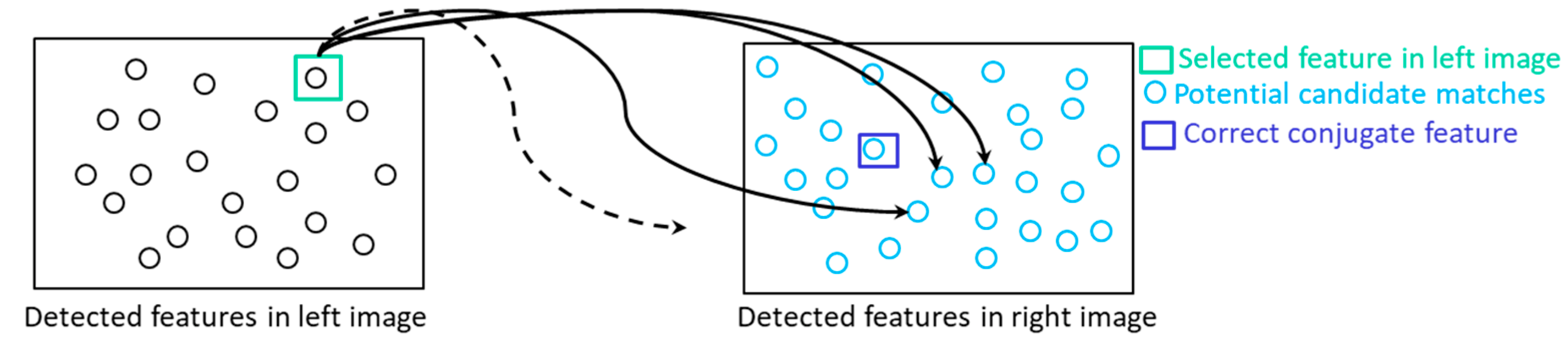
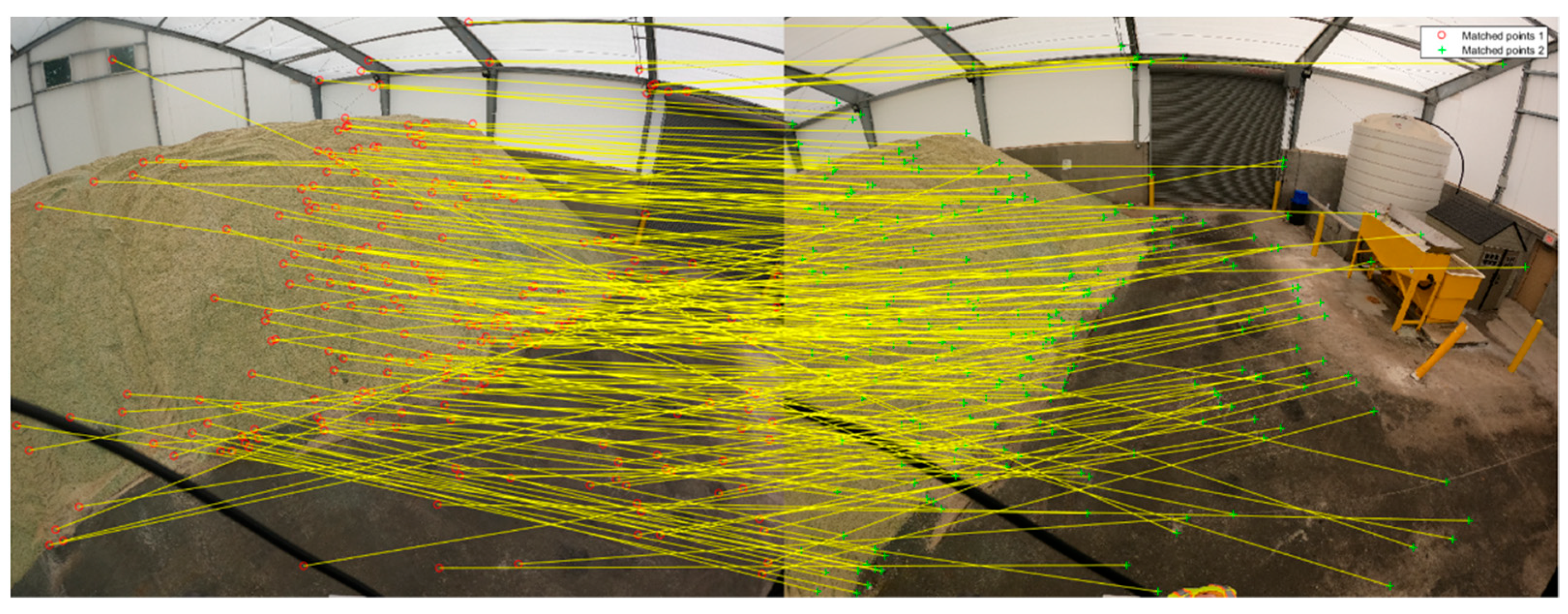
  • Number of matches/projection residuals: For the automated approaches, the number of matches signifies the ability to establish enough conjugate features between two successive images. In the case of manual measurements, few reliable conjugate points with a relatively good distribution are established. The projection residual, which is the RMSE value of differences between the coordinates of projected features from the left to right image and their corresponding features in the right image, can be used to infer the quality of established matches and/or estimated rotation angles. Large projection residual is an indication of high percentage of matching outliers, and consequently, inaccurate estimates of the incremental pole rotation angles.
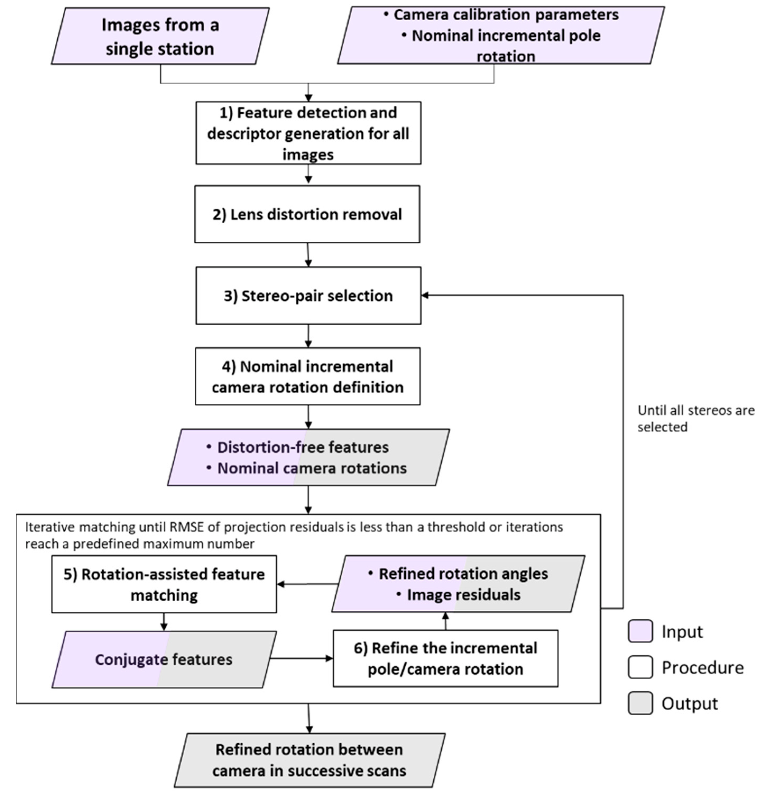
  • Incremental pole rotation angles ( Δ ω , Δ φ , and Δ κ ): Considering the results form manual measurements as a reference, this criterion shows how accurately the automated approaches can estimate the incremental pole rotation between two scans. As mentioned earlier, the nominal incremental pole rotation between two scans (i.e., Δ ω , Δ φ , and Δ κ ) are (0.0°, 0.0°, and −30.0°), respectively.
  • Processing time: For the automated approaches, this refers to the processing time for feature detection, descriptor generation, and matching steps. In case of manual measurements, this refers to the approximate time required for manually identifying point correspondences between the two images.
The above-mentioned evaluation criteria pertaining to the exhaustive/proposed matching approaches and manual measurement of conjugate points for the established six stereo-pairs from the US-231 dataset are presented in Table 4. To show the impact of adopting an iterative process, results from the proposed approach after one iteration, i.e., using only nominal pole rotation angles, are also reported in Table 4. To differentiate the rotation-constrained approaches without and with iterations, they are referred to as one-step constrained and iterative constrained matching, respectively.
In terms of number of matches, the exhaustive approach produces the largest set of conjugate points for all six stereo-pairs. However, looking into the reported projection residuals in Table 4, one can observe that the exhaustive approach leads to significantly larger errors up to ~8000 pixels. Such large projection residual indicates a high percentage of outliers in the conjugate points established by the traditional approach as well as imprecise estimation of the incremental rotation angles. As expected, among the automated approaches, the iterative constrained approach results in the smallest projection residual. In other words, RMSE of the residuals for this approach is always smaller than the selected threshold for stopping the iteration in the proposed iterative matching (i.e., 40 pixels in these experiments). The approach with one iteration, i.e., one-step constrained, results in RMSE values comparable to the iterative strategy in most cases with the exception of stereo-pair 3. Looking into the estimated incremental pole rotations for Stereo-Pair 3 using the manual measurements, it can be seen that the pole rotation angle Δ κ between the two images, which is −43.6°, is significantly different from the nominal rotation angle of −30.0°. Thus, when using nominal rotation angles that are different from the actual ones for deriving the matching search window, the proposed approach leads to some matching outliers in the first iteration, resulting in a large projection error (230 pixels). However, the iterative approach progressively derives more reliable matches and better estimates of the incremental rotation angles. In terms of incremental pole rotation angles, the iterative constrained approach always derives estimates that are quite similar to those using manually-established conjugate points (with differences less than 0.1°). On the other hand, the estimated rotation angles from the exhaustive and one-step constrained approaches differ from the manual measurement results by as much as 4–5° (refer to the values in red for stereo-pair 3). For the processing time, it can be observed that the exhaustive matching is faster than the proposed iterative image matching strategy. The difference in the performance is mainly due to the projection of extracted SIFT features from the left to the right images of a stereo-pair throughout the iterations. The time consumption of the iterative constrained matching approach when compared to the one-step constrained matching depends on the number of iterations. For example, in Stereo-pairs 1 to 5, the processing time for the iterative constrained approach is almost double of that for the one-step constrained matching, indicating that the algorithm met the residual threshold (40 pixels) after two iterations. For Stereo-pair 6, the results show that the iterative constrained approach is identical in performance to the one-step constrained matching. This is due to the fact that the nominal and true rotation angles are very similar for this stereo-pair; thus, the proposed approach reached the projection residual threshold in just one iteration. Overall, from Table 4, it can be concluded that, without a significant increase in the processing time, the proposed image matching strategy can lead to more accurate estimates of the incremental pole rotation angles.
For coarse registration of LiDAR scans at a given station, the rotation from each subsequent scan to the reference frame is derived incrementally. In this regard, one should note that any error in the estimated incremental rotation angles for a given scan will propagate to the following scans. Image-based LiDAR coarse registration results from the exhaustive, one-step constrained, and iterative constrained approaches are illustrated in Figure 23a–c, respectively, for the SMART station in the US-231 dataset. In this figure, point clouds are colored by their respective scan ID (seven scans in total). Through Table 4 and Figure 23, one can conclude that the misalignment in the point clouds resulting from the exhaustive and one-step constrained approaches is mainly caused by an error in the estimated pole rotation for Stereo-pair 3. Through a closer inspection of Figure 23, it can be seen that other than a large error in the Δ κ angle (misalignment shown in the top-view display in Figure 23a), large Δ ω error is also present in the point cloud generated from the exhaustive matching strategy (misalignment shown in the side-view display in Figure 23a). These erroneous incremental rotations are highlighted in Table 4 for the estimated pole rotations for Stereo-pair 3. In summary, the proposed iterative approach leads to point clouds with better alignment when compared to the exhaustive matching and one-step constrained approach.

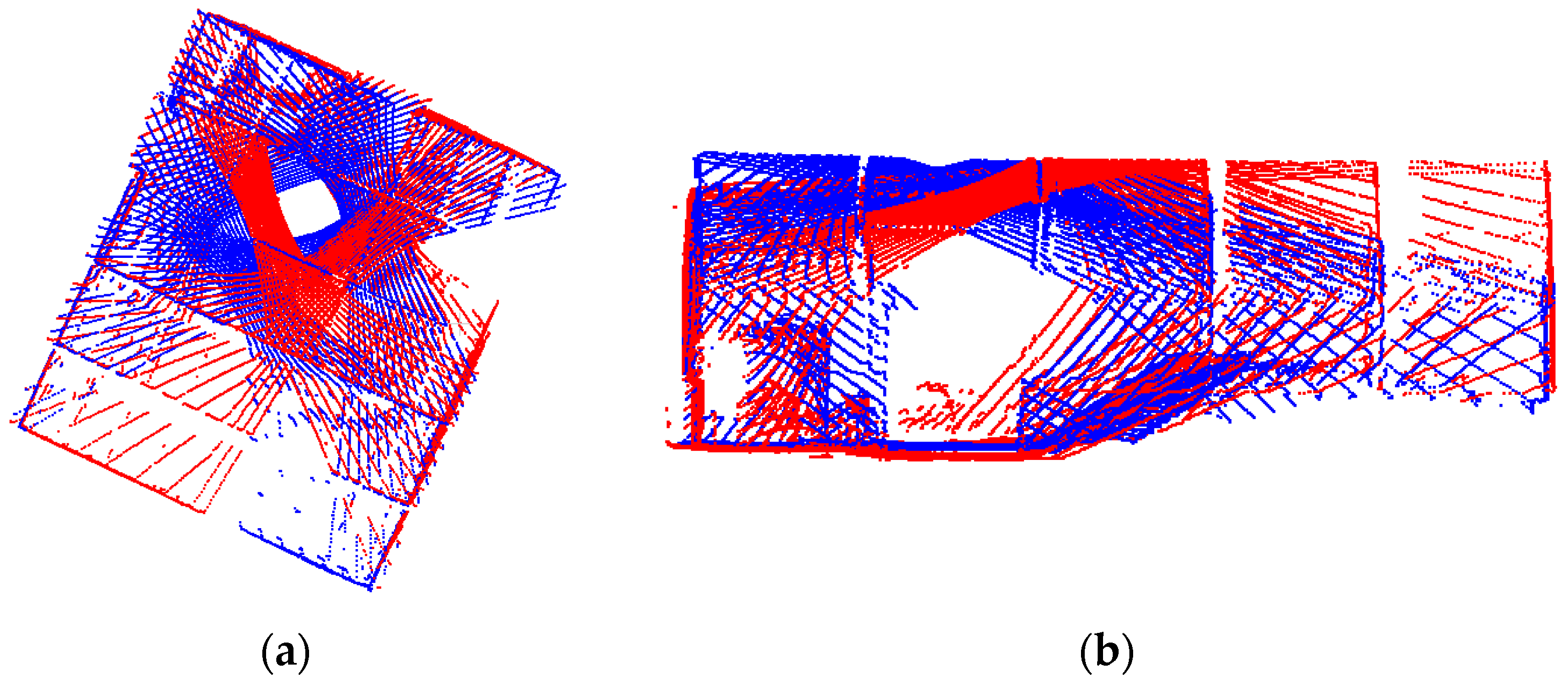
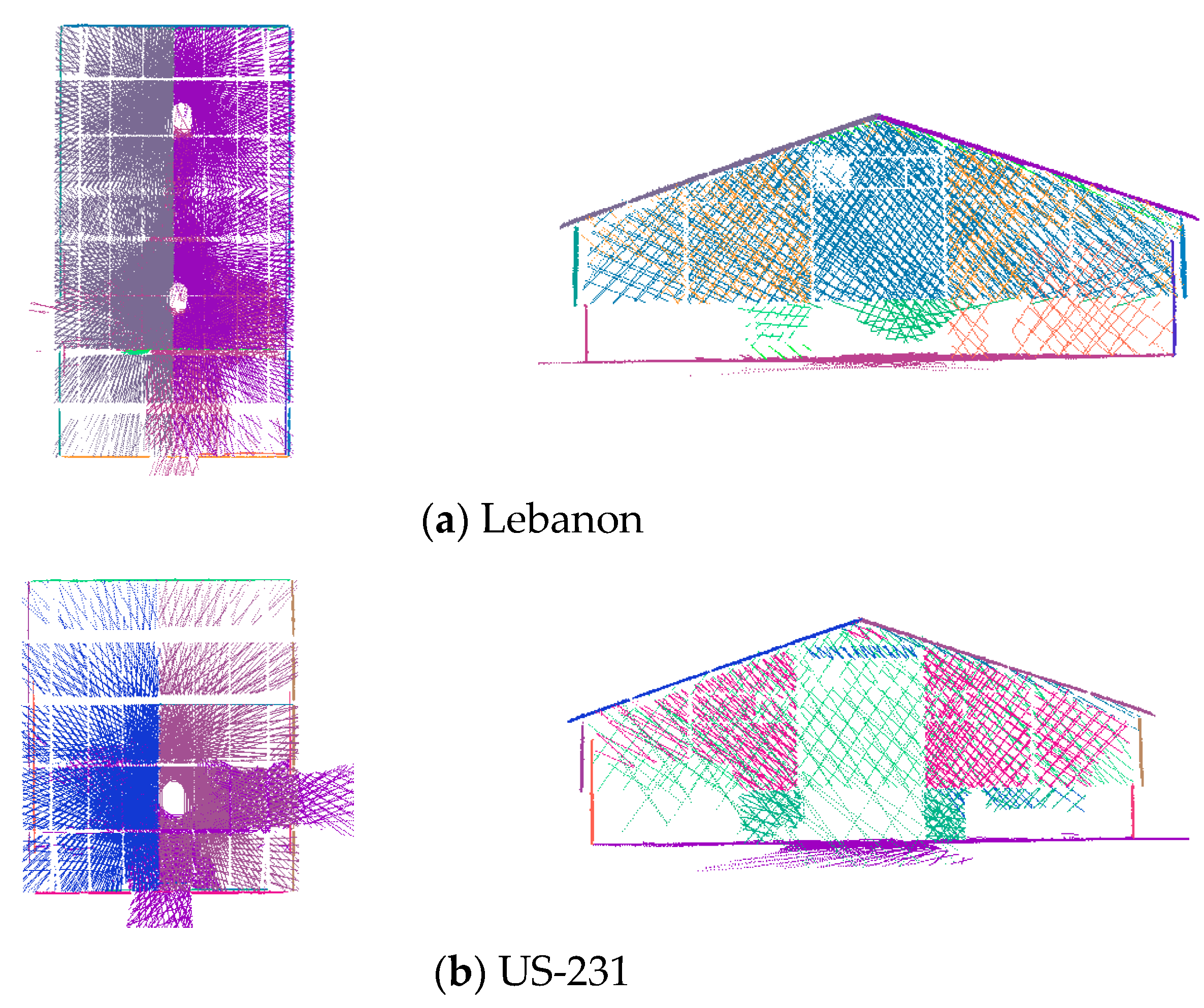
5.3. Fine Registration Results

The reconstructed point clouds after fine registration were assessed using the RMSE of normal distances between post-registered point clouds along the different features and their respective best-fit planes. Results from the SLS-based fine registration for the US-231 and Lebanon datasets are shown in Table 5. In spite of having the same number of planar features, the Lebanon dataset has almost twice the number of points compared to that of US-231. This can be attributed to the additional data collection station at Lebanon. One should note that, since the facility at Lebanon is larger than the US-231 one, point clouds in the former are sparser. In terms of registration accuracy, both datasets have a similar RMSE of about 0.02 m despite having different point cloud densities. This level of accuracy is consistent with the ranging noise of the LiDAR sensors used in the SMART system [48]. In other words, the registration accuracy was only limited by the noise of the LiDAR sensors and was not impacted by the sparsity of the point clouds.
While the quantitative results are sufficient to highlight the accuracy of fine registration, the final point clouds can also be visually inspected. A qualitative evaluation is also important for assessing occluded portions of the stockpile surfaces in the LiDAR scans. For the two SMART datasets, their fine registered point clouds are visualized in Figure 24. One should note that only planar features, none of which belong to the stockpile surface, are shown. The blind spots at locations where the SMART system was stationed are visible in Figure 24.

5.4. Stockpile Volume Estimation

The two SMART datasets in the Lebanon and US-231 salt storage facilities were acquired from an extended tripod that was over 6 m high. As was mentioned earlier, the volumetric accuracy of the SMART system is evaluated by comparing its volume estimates to that from the Faro Focus TLS. For the Lebanon dataset, TLS point clouds were captured from two stations with the scanner mounted on another extendable tripod with similar scanning height to that for the SMART system as shown in Figure 25. Like any other stockpile measurement strategy, SMART and/or TLS are expected to have some occluded portions. Given similar SMART/TLS scanning height for the Lebanon facility, the occlusion pattern for these systems is expected to be similar. To study the impact of occlusions on volume estimation, the TLS in the US 231 was mounted on a regular tripod, and three scans were acquired with two scans on top of the stockpile, as illustrated in Figure 26. The occlusion patterns for the SMART and TLS units in the Lebanon and US 231 facilities are shown in Figure 27. Before volume estimation, the gaps between the stockpile surface and facility boundaries are filled using a bilinear interpolation, as shown in Figure 28. The estimated volume for the two datasets obtained from the SMART system is compared with those from TLS in Table 6; where occlusion percentages for the SMART and TLS stockpile surfaces are also reported.
The comparison between the TLS and SMART volume estimates in Table 6 illustrates two main observations: (1) the relative performance of SMART and TLS given similar occlusion pattern (Lebanon dataset); and (2) impact of occlusion extent on the estimated volumes (US-231 dataset). For the Lebanon dataset, where the SMART and TLS had comparable occlusion percentage, one can see that they both produce similar volumes. This is an indication of the SMART’s ability to deliver volume estimates that are as precise as those derived from TLS. For the US-231 dataset, on the other hand, the difference percentage is in the range of 3%, which is a direct result of higher occlusion percentage for the SMART system.
Salt Repositioning Test: In the Lebanon facility, a salt repositioning test was performed to further examine the volumetric accuracy attained by the proposed system. Initially, the stockpile consisted of two large heaps on the left and right sides of the facility. Using a bucket loader, two small quantities of salt were picked and moved into two new piles (Figure 29). The shapes of the original and repositioned salt piles are shown in Figure 30. Following the repositioning, another set of scans were captured by the SMART and TLS units.
The post-repositioning individual volumes of the big and small piles are assessed using the SMART and TLS scans (Table 7 and Table 8 show the estimates for the left and right piles, respectively). From Table 7 and Table 8, it can be observed that for the big piles, volumetric errors are under 1.4%, whereas for the smaller piles, they were 1.7% and 4.7%. The larger error for the right small pile is attributed to the difference in the extent of occlusions between SMART and TLS, as visualized in Figure 31, where the area marked in yellow has no coverage from the TLS (i.e., the SMART estimate is more reliable in this case). The combined volumes after repositioning are subsequently compared with their corresponding initial volumes, as can be seen in Table 9 and Table 10, where a small and consistent volumetric error of under 1.4% was achieved. It is worth noting that a 2 to 3 cm registration discrepancy could result in more than 10 m 3 volumetric error for big piles (i.e., piles with large base coverage). Therefore, volumetric errors are mainly represented as percentages rather than absolute values.

6. Discussion

This study highlights several key findings. For the SMART system, design considerations were vital for safe and convenient data acquisition, especially when dealing with hard to reach, hazardous stockpiles. Comparisons between SMART and TLS volume estimates revealed that under similar occlusion patterns, both systems derive volume estimates that agree in the range of 1%. Therefore, one can conclude that the data acquisition and processing framework is capable of handling the sparsity of the acquired scans (the Lebanon data is sparser than the US-231 one). The study also revealed that the key factor affecting the quality of estimated volumes is the extent of stockpile surface occlusions. It is important to note that the interpolation method used is not a deciding factor when evaluating the performance of SMART system against the TLS in estimating stockpile volumes. This is expected since volume estimates for both systems are derived using the same strategy and criteria. Therefore, careful considerations in system design and setup should be prioritized to reduce the amount of occlusions. For scalable implementation of a stockpile volume estimation technology, in addition to its accuracy and ease of operation, the system cost is another important factor. Among LiDAR-based platforms, TLS are usually the most expensive. The SMART system, owing to the simplicity of its design, is relatively less expensive. Table 11 lists the approximate cost of three different LiDAR-based stockpile mapping platforms based on current market cost.
In this study, stockpile facilities with well-defined planar features have been extensively tested. These types of facilities follow the modern design criteria established by Indiana DOT for its salt stockpile storage facilities. However, the department still operates several of its legacy units that do not follow this design (e.g., the facilities in Figure 32). Therefore, expanding the developed processing strategy to handle such facilities has to be addressed to ensure the availability of an agnostic stockpile volume estimation for all facility types.

7. Conclusions and Recommendations for Future Work

In this paper, a new mapping system, denoted as Stockpile Monitoring and Reporting Technology (SMART), has been designed for accurate volume estimation of indoor stockpiles. Following the system calibration, the stockpile volume is estimated through six steps: segmentation of planar features from individual scans, image-based coarse registration of LiDAR scans at a single station, feature matching and fine registration of LiDAR point clouds from a single station, coarse registration of point clouds from different stations, feature matching and fine registration of LiDAR point clouds from different stations, and DSM generation for volume estimation. The main contributions of this new system can be summarized as follows:
  • The integrated hardware system composed of an RGB Camera, two LiDAR units, and an extendable tripod. This system addresses the limitations of current stockpile volume estimation techniques by providing a time-efficient, cost-effective, and scalable solution for routine monitoring of stockpiles with varying sizes and shape complexity.
  • An image-aided coarse registration technique has been designed to mitigate challenges in identifying common features in sparse LiDAR scans with insufficient overlap. This new approach uses the designed system characteristics and operation to derive a reliable set of conjugate points in successive images for precise estimation of the incremental pole rotation at a given station.
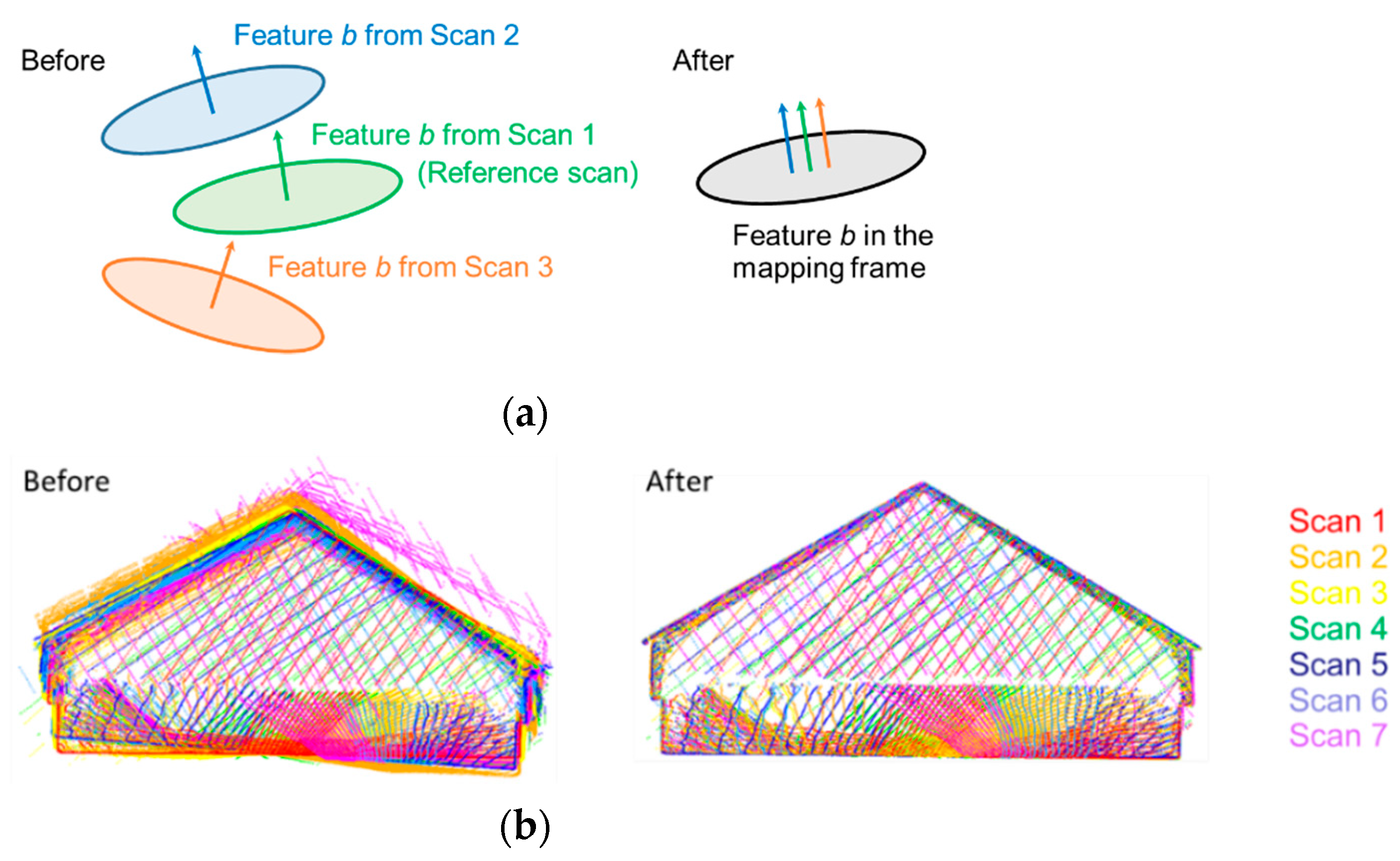
  • A scan line-based segmentation (SLS) approach for extracting planar features from spinning multi-beam LiDAR scans has been proposed. The SLS can handle significant variability in point density and provides a set of planar features that could be used for reliable fine registration.
The developed system and data processing strategy is evaluated through experimental results from two facilities with different size and stockpile storage patterns. For the data processing strategy, the SLS has shown good performance in extracting planar features even when dealing with sparse point clouds leading to fine-registration quality on par with the ranging noise of the used LiDAR units. The image-based coarse registration was successful in deriving a precise set of matched points in successive images and evaluating reliable estimates of incremental pole rotation that are independent of the quality of the nominal values. In general terms, the experimental results have shown that (1) the system design, operation, and data processing strategy are capable of producing volume estimates that are quite similar to those derived from TLS in the range of 1%; and (2) the extent of occlusions is the key factor impacting the quality of volume estimates.
While the experimental results in this paper focused on estimating volume of salt stockpiles, the concepts, development, and analysis are equally applicable for other stockpile volume estimation. Moreover, for outdoor environments, the RTK-GNSS module can be used to provide prior information for coarse and fine registration of point clouds from multiple stations. Similar to any other volume estimation strategy, SMART estimates are affected by the extent of occlusions in the scanned stockpile surface system. Therefore, current and future work will focus on refining the system design and setup to reduce occlusions, including the possibility of hanging/moving the sensor mount along the ceiling of the facility. Moreover, further investigation will be conducted to improve the segmentation performance in facilities with non-planar surfaces.

Author Contributions

Conceptualization, R.M., S.M.H., J.L., Y.K., R.R., and A.H.; methodology, R.M., S.M.H., J.L., Y.-C.L., and A.H.; data acquisition, R.M., Y.K., and J.A.M.; resources, J.A.M., J.M., and T.W.; writing—original draft preparation, R.M., S.M.H., J.L., Y.K., and Y.-C.L.; writing—review and editing, T.Z., R.R., D.B., and A.H.; supervision, D.B. and A.H. All authors have read and agreed to the published version of the manuscript.

Funding

This work was supported in part by the Joint Transportation Research Program administered by the Indiana Department of Transportation (grant number SPR-4549) and Purdue University. The contents of this paper reflect the views of the authors, who are responsible for the facts and the accuracy of the data presented herein, and do not necessarily reflect the official views or policies of the sponsoring organizations. These contents do not constitute a standard, specification, or regulation.

Institutional Review Board Statement

Not applicable.

Informed Consent Statement

Not applicable.

Data Availability Statement

Data sharing is not applicable to this paper.

Acknowledgments

The authors would like to acknowledge the technical and administrative support from the Digital Photogrammetry Research Group (DPRG) members throughout the data collection and data calibration. In addition, we thank the editor and three anonymous reviewers for providing helpful comments and suggestions which substantially improved the manuscript.

Conflicts of Interest

The authors declare no conflict of interest.

References

  1. Desai, J.; Mahlberg, J.; Kim, W.; Sakhare, R.; Li, H.; McGuffey, J.; Bullock, D.M. Leveraging Telematics for Winter Operations Performance Measures and Tactical Adjustment. J. Transp. Technol. 2021, 11, 611–627. [Google Scholar] [CrossRef]
  2. FHWA Road Weather Management Program. Available online: https://ops.fhwa.dot.gov/weather/weather_events/snow_ice.htm (accessed on 23 October 2021).
  3. Kuemmel, D.; Hanbali, R. Accident Analysis of Ice Control Operations. In Transportation Research Center: Accident Analysis of Ice Control Operations; Marquette University: Milwaukee, WI, USA, 1992. [Google Scholar]
  4. Ketcham, S.; Minsk, L.D.; Blackburn, R.R.; Fleege, E.J. Manual of Practice for an Effective Anti-Icing Program: A Guide for Highway Winter Maintenance Personnel; No. FHWA-RD-95-202; Federal Highway Administration: Washington, DC, USA, 1996.
  5. State of New Hampshire Department of Transportation. Winter Maintenance Snow Removal and Ice Control Policy; New Hampshire Department of Transportation: Concord, NH, USA, 2001. Available online: https://www.nh.gov/dot/org/operations/highwaymaintenance/documents/WinterMaintSnowandIcePolicy.pdf (accessed on 19 November 2021).
  6. Mayfield, M.; Narayanaswamy, K.; Jackson, D.W.; Systematics, C. Determining the State of the Practice in Data Collection and Performance Measurement of Stormwater Best Management Practices; U.S. Department of Transportations: Washington, DC, USA, 2014.
  7. Steinfeld, D.E.; Riley, S.A.; Wilkinson, K.M.; Landis, T.D.; Riley, L.E. Roadside Revegetation: An Integrated Approach to Establishing Native Plants (No. FHWA-WFL/TD-07-005); United States Federal Highway Administration, U.S. Department of Transportation: Washington, DC, USA, 2007.
  8. Iyer, A.V.; Dunlop, S.R.; Senicheva, O.; Thakkar, D.J.; Yan, R.; Subramanian, K.; Vasu, S.; Siddharthan, G.; Vasandani, J.; Saurabh, S. Improve and Gain Efficiency in Winter Operations; Joint Transportation Research Program Publication No. FHWA/IN/JTRP-2021/11; Purdue University: West Lafayette, IN, USA, 2021. [Google Scholar] [CrossRef]
  9. He, H.; Chen, T.; Zeng, H.; Huang, S. Ground Control Point-Free Unmanned Aerial Vehicle-Based Photogrammetry for Volume Estimation of Stockpiles Carried on Barges. Sensors 2019, 19, 3534. [Google Scholar] [CrossRef] [PubMed] [Green Version]
  10. Yilmaz, H.M. Close Range Photogrammetry in Volume Computing. Exp. Tech. 2010, 34, 48–54. [Google Scholar] [CrossRef]
  11. Berra, E.F.; Peppa, M.V. Advances and Challenges of UAV SFM MVS Photogrammetry and Remote Sensing: Short Review. In Proceedings of the IEEE Latin American GRSS & ISPRS Remote Sensing Conference (LAGIRS), Santiago, Chile, 22–26 March 2020. [Google Scholar] [CrossRef]
  12. Mora, O.E.; Chen, J.; Stoiber, P.; Koppanyi, Z.; Pluta, D.; Josenhans, R.; Okubo, M. Accuracy of Stockpile Estimates Using Low-Cost sUAS Photogrammetry. Int. J. Remote Sens. 2020, 41, 4512–4529. [Google Scholar] [CrossRef]
  13. Fay, L.; Akin, M.; Shi, X.; Veneziano, D. Revised Chapter 8, Winter Operations and Salt, Sand and Chemical Management, of the Final Report on NCHRP 25-25(04). In Western Transportation Institute; Montana State University: Bozeman, MT, USA, 2013. [Google Scholar]
  14. Hugenholtz, C.H.; Walker, J.; Brown, O.; Myshak, S. Earthwork Volumetrics with an Unmanned Aerial Vehicle and Softcopy Photogrammetry. J. Surv. Eng. 2015, 141, 06014003. [Google Scholar] [CrossRef]
  15. United States Department of Labor Mine Safety and Health Administration. Sand, Gravel, and Crushed Stone on-the-Job Training Modules. MSHA IG-40. 2000. Available online: https://arlweb.msha.gov/training/part46/ig40/ig40.htm (accessed on 19 November 2021).
  16. Arango, C.; Morales, C.A. Comparison between Multicopter UAV and Total Station for Estimating Stockpile Volumes. In Proceedings of the International Conference on Unmanned Aerial Vehicles in Geomatics, Toronto, ON, Canada, 30 August–2 September 2015. [Google Scholar] [CrossRef] [Green Version]
  17. Raeva, P.L.; Filipova, S.L.; Filipov, D.G. Volume Computation of a Stockpile—A Study Case Comparing GPS and UAV Measurements in an Open Pit Quarry. In Proceedings of the XXIII ISPRS Congress, Prague, Czech Republic, 12–19 July 2016; pp. 999–1004. [Google Scholar] [CrossRef] [Green Version]
  18. Khomsin; Pratomo, D.G.; Anjasmara, I.M.; Ahmad, F. Analysis of the Volume Comparation of 3′S (TS, GNSS and TLS). In Proceedings of the E3S Web of Conferences, EDP Sciences, Online, 8 May 2019; Volume 94. [Google Scholar] [CrossRef]
  19. Ajayi, O.G.; Ajulo, J. Investigating the Applicability of Unmanned Aerial Vehicles (UAV) Photogrammetry for the Estimation of the Volume of Stockpiles. Quaest. Geogr. 2021, 40, 25–38. [Google Scholar] [CrossRef]
  20. Luo, Y.; Chen, J.; Xi, W.; Zhao, P.; Qiao, X.; Deng, X.; Liu, Q. Analysis of Tunnel Displacement Accuracy with Total Station. Meas. J. Int. Meas. Confed. 2016, 83, 29–37. [Google Scholar] [CrossRef]
  21. Zhu, J.; Yang, J.; Fan, J.; Danni, A.; Jiang, Y.; Song, H.; Wang, Y. Accurate Measurement of Granary Stockpile Volume Based on Fast Registration of Multi-Station Scans. Remote Sens. Lett. 2018, 9, 569–577. [Google Scholar] [CrossRef]
  22. Little, M.J. Slope Monitoring Strategy at PPRust Open Pit Operation. In Proceedings of the International Symposium on Stability of Rock Slopes in Open Pit Mining and Civil Engineering, Cape Town, South Africa, 3–6 April 2006; The South African Institute of Mining and Metallurgy: Cape Town, South Africa, 2006; pp. 211–230. [Google Scholar]
  23. Campos, M.B.; Litkey, P.; Wang, Y.; Chen, Y.; Hyyti, H.; Hyyppä, J.; Puttonen, E. A Long-Term Terrestrial Laser Scanning Measurement Station to Continuously Monitor Structural and Phenological Dynamics of Boreal Forest Canopy. Front. Plant Sci. 2021, 11, 2132. [Google Scholar] [CrossRef]
  24. Voordendag, A.B.; Goger, B.; Klug, C.; Prinz, R.; Rutzinger, M.; Kaser, G. Automated and Permanent Long-Range Terrestrial Laser Scanning in a High Mountain Environment: Setup and First Results. ISPRS Ann. Photogramm. Remote Sens. Spat. Inf. Sci. 2021, 2, 153–160. [Google Scholar] [CrossRef]
  25. Christie, G.A.; Kochersberger; Abbott, B.; Westman, A.L. Image-Based 3D Reconstructions for Stockpile Volume Measurement. Min. Eng. 2015, 67, 34–37. [Google Scholar]
  26. Rhodes, R.K. UAS as an Inventory Tool: A Photogrammetric Approach to Volume Estimation. Master’s Thesis, University of Arkansas, Fayetteville, AR, USA, 2017. [Google Scholar]
  27. Idrees, A.; Heeto, F. Evaluation of UAV-Based DEM for Volume Calculation. J. Univ. Duhok 2020, 23, 11–24. [Google Scholar] [CrossRef]
  28. Ajayi, O.G.; Oyeboade, T.O.; Samaila-Ija, H.A.; Adewale, T.J. Development of a UAV-Based System for the Semi-Automatic Estimation of the Volume of Earthworks. Rep. Geod. Geoinform. 2020, 110, 21–28. [Google Scholar] [CrossRef]
  29. Long, N.Q.; Nam, B.X.; Cuong, C.X.; van Canh, L. An Approach of Mapping Quarries in Vietnam Using Low-Cost Unmanned Aerial Vehicles. J. Pol. Miner. Eng. Soc. 2019, 2, 248–262. [Google Scholar] [CrossRef]
  30. Liu, S.; Yu, J.; Ke, Z.; Dai, F.; Chen, Y. Aerial–Ground Collaborative 3D Reconstruction for Fast Pile Volume Estimation with Unexplored Surroundings. Int. J. Adv. Robot. Syst. 2020, 17. [Google Scholar] [CrossRef] [Green Version]
  31. Son, S.W.; Kim, D.W.; Sung, W.G.; Yu, J.J. Integrating UAV and TLS Approaches for Environmental Management: A Case Study of a Waste Stockpile Area. Remote Sens. 2020, 12, 1615. [Google Scholar] [CrossRef]
  32. Alsayed, A.; Yunusa-Kaltungo, A.; Quinn, M.K.; Arvin, F.; Nabawy, M.R.A. Drone-Assisted Confined Space Inspection and Stockpile Volume Estimation. Remote Sens. 2021, 13, 3356. [Google Scholar] [CrossRef]
  33. Gago, R.M.; Pereira, M.Y.A.; Pereira, G.A.S. An Aerial Robotic System for Inventory of Stockpile Warehouses. Eng. Rep. 2021, 3, e12396. [Google Scholar] [CrossRef]
  34. Schonberger, J.L.; Frahm, J.M. Structure-from-Motion Revisited. In Proceedings of the IEEE Computer Society Conference on Computer Vision and Pattern Recognition, CVPR 2016, Las Vegas, NV, USA, 27–30 June 2016. [Google Scholar] [CrossRef]
  35. Hasheminasab, S.M.; Zhou, T.; Habib, A. GNSS/INS-Assisted Structure from Motion Strategies for UAV-Based Imagery over Mechanized Agricultural Fields. Remote Sens. 2020, 12, 351. [Google Scholar] [CrossRef] [Green Version]
  36. He, F.; Zhou, T.; Xiong, W.; Hasheminnasab, S.M.; Habib, A. Automated Aerial Triangulation for UAV-Based Mapping. Remote Sens. 2018, 10, 1952. [Google Scholar] [CrossRef] [Green Version]
  37. Hirschmüller, H. Accurate and Efficient Stereo Processing by Semi-Global Matching and Mutual Information. In Proceedings of the IEEE Computer Society Conference on Computer Vision and Pattern Recognition, CVPR 2005, San Diego, CA, USA, 20–25 June 2005; Volume 2. [Google Scholar] [CrossRef]
  38. Furukawa, Y.; Ponce, J. Accurate, Dense, and Robust Multiview Stereopsis. IEEE Trans. Pattern Anal. Mach. Intell. 2010, 32, 1362–1376. [Google Scholar] [CrossRef]
  39. Lowe, D.G. Distinctive Image Features from Scale-Invariant Keypoints. Int. J. Comput. Vis. 2004, 60, 91–110. [Google Scholar] [CrossRef]
  40. Bay, H.; Ess, A.; Tuytelaars, T.; van Gool, L. Speeded-Up Robust Features (SURF). Comput. Vis. Image Underst. 2008, 110, 346–359. [Google Scholar] [CrossRef]
  41. Alcantarilla, P.F.; Nuevo, J.; Bartoli, A. Fast Explicit Diffusion for Accelerated Features in Nonlinear Scale Spaces. In Proceedings of the BMVC 2013—Electronic Proceedings of the British Machine Vision Conference, Bristol, UK, 9–13 September 2013. [Google Scholar]
  42. Li, R.; Liu, J.; Zhang, L.; Hang, Y. LIDAR/MEMS IMU Integrated Navigation (SLAM) Method for a Small UAV in Indoor Environments. In Proceedings of the 2014 DGON Inertial Sensors and Systems, Karlsruhe, Germany, 16–17 September 2014. [Google Scholar]
  43. Youn, W.; Ko, H.; Choi, H.; Choi, I.; Baek, J.H.; Myung, H. Collision-Free Autonomous Navigation of a Small UAV Using Low-Cost Sensors in GPS-Denied Environments. Int. J. Control. Autom. Syst. 2021, 19, 953–968. [Google Scholar] [CrossRef]
  44. HOVERMAP(TM). Available online: https://www.emesent.io/hovermap/ (accessed on 19 November 2021).
  45. Kuhar, M.S. Technology Beyond Measure: New System for Calculating Stockpile Volume Via Smartphone May be a Game-Changer. Rock Prod. 2013, 116, 36–39. Available online: https://web.archive.org/web/20200129142605/http://www.rockproducts.com/index.php/technology/loadout-a-transportation/12343-technology-beyond-measure.html (accessed on 19 November 2021).
  46. Boardman, D.; Erignac, C.; Kapaganty, S.; Frahm, J.-M.; Semerjian, B. Determining Object Volume from Mobile Device Images. U.S. Patent No. 9,196,084, 24 November 2015. [Google Scholar]
  47. Stockpile Reports Inventory Measurement App Delivers Instant Results. Rock Products. 2020, Volume 123, p. 37. Available online: https://link.gale.com/apps/doc/A639274390/AONE (accessed on 19 November 2021).
  48. Velodyne VLP16 Puck. Available online: https://velodynelidar.com/products/puck/ (accessed on 3 November 2021).
  49. He, F.; Habib, A. Target-Based and Feature-Based Calibration of Low-Cost Digital Cameras with Large Field-of-View. In Proceedings of the Imaging and Geospatial Technology Forum, IGTF 2015—ASPRS Annual Conference and co-located JACIE Workshop, Tampa, FL, USA, 4–8 May 2015. [Google Scholar]
  50. Ravi, R.; Lin, Y.J.; Elbahnasawy, M.; Shamseldin, T.; Habib, A. Simultaneous System Calibration of a Multi-LiDAR Multicamera Mobile Mapping Platform. IEEE J. Sel. Top. Appl. Earth Obs. Remote Sens. 2018, 11, 1694–1714. [Google Scholar] [CrossRef]
  51. Zhou, T.; Hasheminasab, S.M.; Habib, A. Tightly-Coupled Camera/LiDAR Integration for Point Cloud Generation from GNSS/INS-Assisted UAV Mapping Systems. ISPRS J. Photogramm. Remote Sens. 2021, 180, 336–356. [Google Scholar] [CrossRef]
  52. Nistér, D. An Efficient Solution to the Five-Point Relative Pose Problem. IEEE Trans. Pattern Anal. Mach. Intell. 2004, 26, 756–770. [Google Scholar] [CrossRef] [PubMed]
  53. Horn, B.K.P. Closed-Form Solution of Absolute Orientation Using Unit Quaternions. J. Opt. Soc. Am. A 1987, 4, 629–642. [Google Scholar] [CrossRef]
  54. Mikolajczyk, K.; Schmid, C. A Performance Evaluation of Local Descriptors. IEEE Trans. Pattern Anal. Mach. Intell. 2005, 27, 1615–1630. [Google Scholar] [CrossRef] [PubMed] [Green Version]
  55. Schmid, C.; Mohr, R.; Bauckhage, C. Evaluation of Interest Point Detectors. Int. J. Comput. Vis. 2000, 37, 151–172. [Google Scholar] [CrossRef] [Green Version]
  56. Karami, E.; Prasad, S.; Shehata, M. Image matching using SIFT, SURF, BRIEF and ORB: Performance comparison for distorted images. arXiv 2017, arXiv:1710.02726. [Google Scholar]
  57. Lin, Y.-C.; Liu, J.; Cheng, Y.-T.; Hasheminasab, S.M.; Wells, T.; Bullock, D.; Habib, A. Processing Strategy and Comparative Performance of Different Mobile LiDAR System Grades for Bridge Monitoring: A Case Study. Sensors 2021, 21, 7550. [Google Scholar] [CrossRef]
  58. Sampath, A.; Shan, J. Building Boundary Tracing and Regularization from Airborne Lidar Point Clouds. Photogramm. Eng. Remote Sens. 2007, 73, 805–812. [Google Scholar] [CrossRef] [Green Version]
  59. Kwak, E.; Habib, A. Automatic Representation and Reconstruction of DBM from LiDAR Data Using Recursive Minimum Bounding Rectangle. ISPRS J. Photogramm. Remote Sens. 2014, 93, 171–191. [Google Scholar] [CrossRef]
  60. OpenCV. Open-Source Computer Vision Library. 2015. Available online: https://opencv.org/ (accessed on 19 November 2021).
Figure 1. The integrated SMART system with all its major components. System setup for data acquisition within an indoor facility is shown on the left.
Remotesensing 14 00231 g001
Figure 2. Horizontal coverage of the LiDAR units and RGB camera on the SMART system.
Remotesensing 14 00231 g002
Figure 3. Integration scheme for the SMART system components.
Remotesensing 14 00231 g003
Figure 4. Illustration of SMART system rotation at a given station. Scan 1 to 7 leads to a 180° rotation of the pole in approximately 30° increments.
Remotesensing 14 00231 g004
Figure 5. Locations of surveyed salt storage facilities: Lebanon unit and US-231 unit of West Lafayette, both in Indiana, USA.
Remotesensing 14 00231 g005
Figure 6. Workflow of the proposed stockpile volume estimation using the SMART system. * MBR: minimum bounding rectangle.
Remotesensing 14 00231 g006
Figure 7. Schematic diagram illustrating the point positioning equations for 3D reconstruction using camera and LiDAR units mounted on the SMART system. For a better visualization of system parameters, the camera and LiDAR units are depicted much farther from the pole compared to their actual mounting positions.
Remotesensing 14 00231 g007
Figure 8. Example of varying orientation of planar features and significant variability in point density in one scan from the SMART system, colored by height. The TLS point cloud of the facility colored by RGB is shown in the upper left box.
Remotesensing 14 00231 g008
Figure 9. Illustration of the proposed SLS strategy with points pertaining to two smooth curve segments. A set of sequentially scanned points is assumed to consist of five points and the outlier threshold n T is set to 2.
Remotesensing 14 00231 g009
Figure 10. Sample results for the SLS approach: (a) point cloud from a single beam scan, (b) smooth curve segments along the same point cloud (different curve segments are in different colors), (c) derived smooth curve segments from all laser beams in a LiDAR scan (different curve segments are in different colors), and (d) planar feature segmentation results (different planar features are in different colors).
Remotesensing 14 00231 g010
Figure 11. Coarse registration results using nominal rotation angles for two scans ( k = 3 and k = 5 ) in the US-231 dataset: (a) top-view and (b) side view. Point clouds are colored by scan ID.
Remotesensing 14 00231 g011
Figure 12. Traditional exhaustive matching strategy: each feature descriptor in the left image is compared with all feature descriptors in the right image.
Remotesensing 14 00231 g012
Figure 13. Sample exhaustive matching results with several outliers for a stereo-pair in the US-231 dataset (for a better visualization only 10% of matches are illustrated).
Remotesensing 14 00231 g013
Figure 14. Flowchart of the proposed rotation-constrained image matching for the SMART system.
Remotesensing 14 00231 g014
Figure 15. Rotation-constrained image matching: (a) predicted point location and matching search window size in first iteration and (b) progression of the matching evaluation through the iterations.
Remotesensing 14 00231 g015
Figure 16. Sample matching results for a stereo-pair in the US-231 dataset: (a) rotation-constrained matching after one iteration with 513 matches and projection residual of 230 pixels and (b) rotation-constrained approach after two iterations with 2127 matches and projection residual of 25 pixels (for a better visualization, only 10% of matches are illustrated).
Remotesensing 14 00231 g016
Figure 17. Image-based coarse registration results for two scans (k = 3 and k = 5) of the single station in US-231 dataset, which had been originally aligned using the nominal pole rotation angle (Figure 11): (a) top-view and (b) side view. Point clouds are colored by scan ID.
Remotesensing 14 00231 g017
Figure 18. Illustration of feature-based fine registration: (a) conceptual basis of using planar features for fine registration and (b) sample point cloud (with seven scans) before and after registration with each scan represented by a single color.
Remotesensing 14 00231 g018
Figure 19. Example boundary tracing of a facility. (a) Boundary points extracted from projected point cloud and (b) defined MBR for the boundary points.
Remotesensing 14 00231 g019
Figure 20. Schematic illustration of stockpile surface generation and volume estimation.
Remotesensing 14 00231 g020
Figure 21. Sample images captured by the SMART system inside the site used for evaluating the inter-sensor mounting parameters.
Remotesensing 14 00231 g021
Figure 22. Point clouds from the two LiDAR units for a given scan before (left) and after (right) system calibration (point clouds are colored by LiDAR unit).
Remotesensing 14 00231 g022
Figure 23. Top-view (left column) and side-view (right column) of coarse registration results for the SMART station in the US-231 dataset using parameters derived from: (a) exhaustive matching, (b) one-step constrained matching, and (c) iterative constrained matching. Point clouds are colored by their respective scan ID.
Remotesensing 14 00231 g023
Figure 24. Fine-registered point cloud from the proposed SLS-based approach, visualized from top view (left) and front view (right). Only the features used in registration are shown (point clouds are colored by their respective planar features).
Remotesensing 14 00231 g024
Figure 25. FARO Focus on an extendable tripod inside the Lebanon Facility.
Remotesensing 14 00231 g025
Figure 26. Illustration of TLS acquisition stations in the US-231 facility: schematic top view (left); TLS setup on top of the stockpile (right).
Remotesensing 14 00231 g026
Figure 27. Stockpile surface occlusions from the SMART and TLS for Lebanon (left) and US-231 (right) facilities. Facility boundaries are indicated in red (point clouds are colored by height). Triangular markers are scan stations of the corresponding platforms.
Remotesensing 14 00231 g027
Figure 28. Stockpile surfaces from SMART before and after interpolation. Original point cloud after fine registration (left) and point cloud after surface interpolation (right): point cloud colored by height.
Remotesensing 14 00231 g028
Figure 29. Salt repositioning experiment at the Lebanon facility.
Remotesensing 14 00231 g029
Figure 30. Top view of RGB color-coded point clouds from the TLS, acquired before/after salt repositioning test at the Lebanon Facility. Initial left and right piles are highlighted in red and blue, respectively (left), along with the corresponding small and big piles after repositioning (right).
Remotesensing 14 00231 g030
Figure 31. Point clouds for the right small pile in the Lebanon facility from TLS and SMART highlighted in red and blue, respectively. Top view (left), and side view (right).
Remotesensing 14 00231 g031
Figure 32. Examples of warehouses with non-planar building structures (left) and segmented LiDAR scan (right) (point clouds are colored by feature).
Remotesensing 14 00231 g032
Table 1. Summary of pros and cons of current mapping/surveying techniques along with the proposed SMART for routine stockpile monitoring.
Operator’s
Safety
ScalabilityFeatureless SurfacesCost-EffectiveIndoorOperator’s Skill
Total StationHigh
RTK-GNSSLow
Terrestrial PhotogrammetryLow
Terrestrial LiDARLow
UAV PhotogrammetryLow
UAV LiDARHigh
SMARTLow
Table 2. Summary of the captured salt storage facilities.
Salt Storage
Facility
SMARTFaro Focus (TLS)Size (W × L × H)
Number of StationsNumber of Scans Per StationNumber of
Stations
Lebanon unit27226 m × 48 m × 10.5 m
US-231 unit17330.5 m × 25.5 m × 10 m
Table 3. Estimated mounting parameters relating the LiDAR and camera units to the pole coordinate frame.
SensorLever-Arm OffsetBoresight Angles
ΔX (m)ΔY (m)ΔZ (m)Δω(°)Δφ(°)Δκ(°)
LiDAR Unit 10−0.2004200
LiDAR Unit 2−0.165−0.029−0.072−7.102−57.144−104.146
(Std. Dev.)±0.001±0.0004±0.001±0.004±0.002±0.004
Camera0.017−0.0340.024−14.686−66.394−103.886
(Std. Dev.)±0.014±0.015±0.020±0.787±0.288±0.801
Table 4. Performance comparison of the traditional and proposed image matching techniques in terms of number of matches, processing time, projection residual, and estimated relative pole rotations for the station in the US-231 dataset.
Image-Based Coarse Registration TechniqueStereo
(Image) ID
Number of MatchesProjection
Residuals (Pixel)
Pole Δω(°)Pole Δφ(°)Pole Δκ(°)Processing Time (Second)
Exhaustive1
(1–2)
34663481.10.1−22.32.06
One-step constrained1922661.50.2−22.839.00
Iterative constrained3408251.50.2−22.581.19
Manual measurements11101.50.3−22.4~600
Exhaustive2
(2–3)
31594471.6−0.5−22.62.10
One-step constrained2065400.8−0.5−23.633.14
Iterative constrained3079290.9−0.5−23.672.33
Manual measurements1080.8−0.5−23.6~420
Exhaustive3
(3–4)
239440424.9−1.2−40.61.99
One-step constrained513230−2.80.9−38.321.15
Iterative constrained2127251.2−0.2−43.644.47
Manual measurements1271.2−0.1−43.6~540
Exhaustive4
(4–5)
279882445.1−2.8−36.62.04
One-step constrained1744761.0−0.5−38.225.41
Iterative constrained2506321.1−0.6−38.449.62
Manual measurements1081.1−0.7−38.4~300
Exhaustive5
(5–6)
40665192.1−0.2−21.22.12
One-step constrained2398470.90.1−22.040.26
Iterative constrained3914341.00.1−21.982.80
Manual measurements1071.20.2−21.9~300
Exhaustive6
(6–7)
368011211.9−0.7−31.42.07
One-step constrained3495271.1−0.4−32.543.83
Iterative constrained3495271.1−0.4−32.542.83
Manual measurements1051.3−0.4−32.5~480
Table 5. Accuracy assessment of post-fine registration of point clouds in the Lebanon and US-231 facilities.
DatasetTotal Number of Planar Features UsedTotal Number of PointsPoint Density Range (Points/m2)RMSE of Normal Distance (m)LiDAR Ranging Noise (m)
Lebanon13516,7562–1890 *0.02110.03
US-23113275,1460.3–7900.0212
* Based on two stations; for one station it is in a range of 0.3–700 points/ m 2 .
Table 6. Comparison of volume estimates from the SMART and TLS scans.
DatasetOcclusion (%)SMART Volume
( m 3 )
TLS Volume ( m 3 ) Difference   ( m 3 ) Error (%)
SMARTTLS
Lebanon31.834.31438.91437.51.4~0.0
US-23149.620.6999.5968.431.13.2
Table 7. SMART and TLS volumes estimates for post-repositioned stockpiles on the left side.
Volume from SMART
( m 3 )
Reference/TLS
( m 3 )
Difference   ( m 3 ) Error (%)
Left big pile798808.910.91.4
Left small pile17.217.50.31.7
Combined left815.2826.411.21.4
Table 8. SMART and TLS volumes estimated for post-repositioned stockpiles on the right side.
Volume from SMART
( m 3 )
Reference/TLS
( m 3 )
Difference   ( m 3 ) Error (%)
Right big pile603.9604.10.2~0.0
Right small pile17.0417.880.844.7
Combined right620.94621.981.040.2
Table 9. SMART and TLS volume estimates for the left pile before/after repositioning.
Initial   Volume   ( m 3 ) Combined   Volume   after   Repositioning   ( m 3 ) Difference
( m 3 )
Error (%)
SMART819.3815.24.10.5
Reference/TLS815.1826.411.31.4
Table 10. SMART and TLS volumes for the right pile before/after repositioning.
Initial   Volume   ( m 3 ) Combined   Volume   after   Repositioning   ( m 3 ) Difference
( m 3 )
Error (%)
SMART619.3620.941.640.3
Reference/TLS622.4621.980.42~0.0
Table 11. Cost comparison of LiDAR-based stockpile mapping platforms.
PlatformApproximate Cost (USD)
SMART ~ 8000
UAV LiDAR30,000+
Terrestrial LiDAR20,000–35,000+
Publisher’s Note: MDPI stays neutral with regard to jurisdictional claims in published maps and institutional affiliations.

