
Multispectral Image Enhancement Based on the Dark Channel Prior and Bilateral Fractional Differential Model


1
The Key Laboratory of Signal Detection and Processing, College of Information Science and Engineering, Xinjiang University, Urumqi 830046, China
2
Institute of Image Processing and Pattern Recognition, Shanghai Jiao Tong University, Shanghai 200400, China
3
Knowledge Engineering and Discovery Research Institute, Auckland University of Technology, Auckland 1020, New Zealand
*
Author to whom correspondence should be addressed.
Remote Sens. 2022, 14(1), 233; https://0-doi-org.brum.beds.ac.uk/10.3390/rs14010233
Submission received: 14 November 2021
/
Revised: 31 December 2021
/
Accepted: 3 January 2022
/
Published: 5 January 2022
(This article belongs to the Special Issue Advances in Optical Remote Sensing Image Processing and Applications)
Abstract
:Compared with single-band remote sensing images, multispectral images can obtain information on the same target in different bands. By combining the characteristics of each band, we can obtain clearer enhanced images; therefore, we propose a multispectral image enhancement method based on the improved dark channel prior (IDCP) and bilateral fractional differential (BFD) model to make full use of the multiband information. First, the original multispectral image is inverted to meet the prior conditions of dark channel theory. Second, according to the characteristics of multiple bands, the dark channel algorithm is improved. The RGB channels are extended to multiple channels, and the spatial domain fractional differential mask is used to optimize the transmittance estimation to make it more consistent with the dark channel hypothesis. Then, we propose a bilateral fractional differentiation algorithm that enhances the edge details of an image through the fractional differential in the spatial domain and intensity domain. Finally, we implement the inversion operation to obtain the final enhanced image. We apply the proposed IDCP_BFD method to a multispectral dataset and conduct sufficient experiments. The experimental results show the superiority of the proposed method over relative comparison methods.
1. Introduction
Recently, multispectral remote sensing images have been widely used in agriculture, forestry, mineral exploration, military, and many other fields, resulting in huge social and economic benefits [1]; however, due to the limitations of sensors and atmospheric scattering, the visual effect and spatial resolution of multispectral remote sensing images cannot fully meet the demands of people; therefore, image enhancement processing is usually used before image analysis and interpretation to highlight useful information and expand the differences between different features [2,3,4]. Multispectral remote sensing images are generated by collecting several bands of the same region in different spectral sampling intervals [5]. The generated data include information from multiple channels.
At present, single-channel image enhancement methods mainly include spatial domain algorithms and frequency domain algorithms [6,7,8]. Common spatial domain algorithms include histogram matching [9,10,11], Retinex algorithms [12,13,14,15], morphological methods [16], differential filtering algorithms, dark channel prior algorithms, and deep learning algorithms.
Differential filtering algorithms include integer-order differential algorithms and fractional differential algorithms. In integer-order differential algorithms, several integer-order operators, including first-order operators, such as the Sobel operator and Prewitt operator, and second-order operators, such as the Laplacian operator [17], have been proposed to sharpen images. With the appearance of fractal theory, fractional differential algorithms have been widely used [18]. Compared with integer-order differential algorithms, fractional differential algorithms can preserve the low-frequency information of the smooth region and the high-frequency edge features [19]. Classic fractional differential algorithms process images in the form of filtering masks; however, the masks usually cannot make full use of the autocorrelation between neighboring pixels [20]. The pixels in the image have great correlations, and these correlations are mainly reflected in the spatial position relations; therefore, some researchers proposed dividing the nonzero coefficients of the fractional differential mask equally within the pixel neighborhood [20,21]; however, the above differential filtering algorithm cannot accurately represent the spatial position relations in the neighborhood and cannot improve the detailed information of smooth areas.
The dark channel prior algorithm, which mainly utilized the deviation of each pixel from the minimum brightness point in the three basic color channels to enhance images and obtain an effective defogging effect for a single image, was proposed by He et al. [22]. Dong et al. [23] found the similarity between low illuminance images after inversion and haze images and applied the dark channel prior theory to low-illuminance image enhancement. At present, researchers have also proposed some methods combining dark channel priors with other algorithms [24,25,26,27,28]; however, the above enhancement algorithms are used for color images or grey images, and the multispectral remote sensing image contains more than three bands. We expand the RGB channels and optimize the transmittance through the fractional differentiation algorithm in the spatial domain.
Furthermore, traditional algorithms have relatively been less used in the field of image enhancement, especially in remote sensing images. In recent years, deep learning algorithms have been widely applied in image enhancement [29]; however, deep learning algorithms still have some disadvantages, such as long training time, large data demand, and low universality.
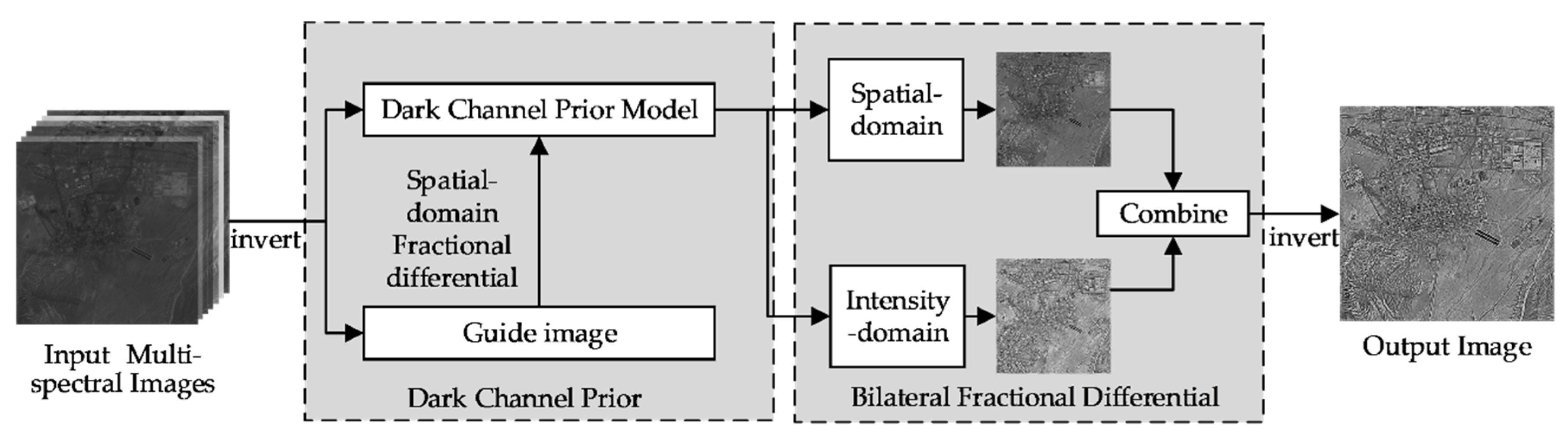
Therefore, an improved enhancement method based on the dark channel prior and fractional differential filtering is proposed. We implement the improved dark channel prior technology to improve the clarity and brightness of the original multispectral image and then use the bilateral fractional differential algorithm to further enhance the edge and textural details of the image. Figure 1 illustrates the flowchart of the proposed method, which contains four steps. The first step is to invert the original multispectral image to make it suitable for dark channel theory. Second, the improved dark channel prior technology is used to enhance the image after inversion. The guided image is obtained by space domain fractional differential filtering and applied to estimate the transmittance of the dark channel prior. Simultaneously, the original channels are extended to multiple channels. Third, a bilateral fractional differential algorithm is proposed to enhance image details, which includes the space domain fractional differential model and intensity domain fractional differential model. Multiple bands of the multispectral image are enhanced by the spatial domain algorithm and intensity domain algorithm. Finally, the combined image is inverted and synthesized to obtain the final enhanced image. To verify the effectiveness of the method, we test and analyze it on multispectral image datasets.
Compared with previous works, our proposed method mainly offers the following contributions.
- (1)
- By synthesizing the multiband information of multispectral remote sensing images, our algorithm obtains more accurate and clearer images than single-band remote sensing images.
- (2)
- A bilateral fractional differential model is firstly proposed and effectively improves the edge and textural details of multispectral images.
- (3)
- By expanding the bands and optimizing the transmittance of the dark channel prior model, an improved image with higher contrast and brightness is further obtained.
The remainder of this paper is organized as follows. Section 2 introduces the related multispectral image enhancement methods. Section 3 describes the principle and implementation steps of the proposed method. Section 4 discusses the experimental datasets and experimental results. Section 5 presents the conclusion.
2. Related Work
In this section, we briefly review previous works on multispectral remote sensing image enhancement.
At present, some enhancement algorithms for multispectral images have been proposed. Tian et al. [30] introduced the extended offset sparsity decomposition (OSD) algorithm into multispectral image enhancement and applied it to hue saturation value (HSV) transformation and principal component analysis (PCA) transformation, respectively, thereby forming the HSV-OSD and the PCA-OSD algorithms, respectively. OSD is performed on the brightness component of HSV and the selected principal component of PCA to maintain the original image information and improve the image details. A. K. Bhandari et al. [31] applied a method combining the discrete wavelet transform (DWT) and singular value decomposition (SVD) to multispectral color image enhancement. The original image was decomposed by the wavelet transform and the subbands were normalized by SVD so that the image after inverse discrete wavelet transform (IDWT) had higher contrast. In addition, A. K. Bhandari et al. [32] presented a combination method of the discrete cosine transform (DCT) and SVD to highlight the contrast of color multispectral remote sensing images. In [33], Shilpa Suresh et al. exploited a novel framework for the enhancement of multispectral images, which primarily aimed to highlight the contrast of color-synthesis remote sensing images through a modified linking synaptic computation network (MLSCN). Wang et al. [34] exploited a color constancy algorithm, which used the improved linear transformation function to improve the brightness while avoiding color distortion. Shan-long Lu et al. [35] introduced a multispectral satellite remote sensing image enhancement algorithm based on the combination of PCA and the intensity-hue-saturation (IHS) transform. The intensity component of the IHS transform was replaced by the first principal component of the PCA transform, and the inverse IHS transform was applied to obtain an enhanced image. T. Venkatakrishnamoorthy et al. [36] mainly expounded on a method based on spatial enhancement and spectral enhancement, which was applied to false-color-synthetic satellite cloud images. The algorithm was used in image processing after extracting useful features using independent component analysis (ICA) and PCA.
Nevertheless, the above research was mainly applied to color-synthetic multispectral images. That is, the images only included three bands of the original multispectral images, which cannot effectively combine the information of other bands. To solve the above problems, some multiband image enhancement algorithms have been proposed. In [37], Afshan Mulla et al. proposed a multispectral image enhancement scheme for specific bands, which performed selective region enhancement to improve the resolution of all bands. Chen Yang et al. [38] proposed a fuzzy PCA algorithm and tested it on a multispectral image dataset with six bands. The algorithm improved the accuracy of surface feature identification by introducing fuzzy statistics; however, the abovementioned studies do not show a satisfactory enhancement effect on image brightness and contrast and cannot sufficiently enhance the edge and local details of images.
In this paper, our proposed method is different from the previous multispectral remote sensing image enhancement methods in the following ways.
- (1)
- The method of combining the dark channel prior algorithm with the fractional differential algorithm is applied to multispectral remote sensing image enhancement for the first time. Based on improving the overall brightness and detail characteristics of the image, the information of the spatial dimension and spectral dimension is combined to make full use of all wave bands of multispectral images.
- (2)
- Unlike the previous fractional differential algorithm, we propose a new fractional differential framework that enhances the edge and textural details of images. Considering the influence of the spatial distance on the pixel autocorrelation, we modify the fractional differential coefficients and propose the spatial domain fractional mask. Furthermore, according to the ability of the pixel similarity to judge the image edge, we propose the intensity domain fractional mask. Then the two above domains are fused to compose the bilateral fractional differential framework, and the enhanced images can be obtained by the framework. This framework can fully combine the information of spatial domain and intensity domain to maintain the details of the image in the smooth region and texture region and improve the image definition.
- (3)
- An improved dark channel prior algorithm, which extends the RGB channels to multiple channels and optimizes the transmittance through our proposed spatial domain fractional differentiation algorithm to make full use of the ground features of different spectral bands and enhance the overall brightness and contrast of an image, is proposed.
3. Proposed Method
In this section, we review the definitions of the classical dark channel prior algorithm and fractional differential algorithm and discuss the principles and steps of the proposed method.
3.1. Dark Channel Prior
An inverted low illumination image and its histogram have high similarities with a hazy image and its histogram [23]; therefore, first, the low illumination image is inverted as
where denotes the pseudohaze image vector containing 3-channel images , and denotes the input image vector containing 3-channel images . The physical model of atmospheric scattering describing haze images can be expressed as
where is the transmittance, which represents the degree of scattering of the incident light; represents the total intensity of atmospheric light; and represents the image vector to be restored containing 3-channel images .
He et al. [22] stated that in most local areas of fog-free images, there are some pixels with very low values in at least one of the color channels; therefore, the dark channel prior theory was proposed. That is, for a fog-free image, the dark channel can be defined as
where represents the dark channel, and is the intensity of the color channels including , , and , represents the filtering window centered on the pixel point.
The rule of the dark channel prior can be defined as
The core of the dark channel prior model is to obtain the atmospheric light and transmittance by handling the dark channel map and then realize image enhancement according to the image defogging model.
To estimate the initial transmittance, the atmospheric scattering model is normalized as
Assuming that the transmittance is constant in the same filtering window, minimum filtering is conducted at both ends of the above formula to obtain the transmittance with errors , which can be written as follows:
Assuming that the image to be restored is similar to the clear image under normal weather conditions, the dark channel prior rule can be generated as
Dividing by the constant , we can obtain
Continuing with the derivation, the transmittance is computed by
Under normal weather conditions, incident light inevitably has some scattering effects, which shows that close objects are displayed more clearly, and distant objects are usually blurrier. To preserve this depth-of-field effect and avoid the over enhancement of images, a constant parameter is introduced to increase the transmittance. The final transmission is modified as
where is the haze removal factor, which is generally set to 0.95.
In the above deduction, it is assumed that the ambient light intensity is known. In practice, we can obtain the value from the dark channel of foggy images. The smaller the reflectivity of a pixel in the image, the greater the attenuation of the incident light, and the greater the superposition effect of ambient light; thus, the grey value of the corresponding pixel is higher in the final dark channel map. The larger the reflectivity of the pixel is, the smaller the attenuation of incident light and the weaker the effect of ambient light. Generally, the grey value of the corresponding pixel is lower. In He’s work, the first 0.1% pixels with the largest brightness values were screened in a dark channel image, that is, the area where the transmittance is close to zero; and then the pixel value of the point with the highest brightness was found as the ambient light value in the corresponding position of the area.
After calculating the atmospheric light and transmittance, the reconstructed image of the real scene can be obtained by substituting the image defrosting model:
A smaller value of the projection map will result in a larger value of , which will make the entire image transition to the white field; therefore, the threshold is written as . When is less than , set , and the typical value of is 0.1. The final haze-free image is recovered by
3.2. Improved Dark Channel Prior
Multispectral remote sensing images usually have the characteristics of low contrast and low illumination; therefore, we reverse the multispectral image and then substitute the haze removal model.
where denotes the pseudofoggy image vector containing multi-channel images , denotes the input image vector containing multi-channel images , and represents the number of bands of the multispectral image. The atmospheric scattering model of multispectral images can be modified as
where represents the image vector to be restored containing multi-channel images .
For a fog-free image, the dark channel can be defined by
where is the intensity of any channel of multispectral image; therefore, the atmospheric scattering model is generated as
In addition, we improve the guided filtering operation in the refinement of the transmittance. We use the image enhanced by the fractional differential algorithm in the spatial domain as the guide image, which can better identify the edge and texture area of the image, remove the image details, and make the guided filtering more accurate.
The improved dark channel image is introduced as
where represents the refinement of the dark image obtained by the spatial domain fractional differential algorithm. We represent the intensity value of pixel coordinate as the in the thinned dark channel image and Equation (17) can be expressed as the convolution of dark channel image and spatial domain fractional differential mask.
where is the original dark channel image, represents the spatial domain fractional mask in Table 3 of Section 3.4.1, is the intensity value of pixel coordinate in the original dark channel image.
Accordingly, the transmittance can be written as follows:
Dividing by a constant , we can obtain the dark channel rule as follows:
The estimated transmittance can be defined as
Therefore, the final enhanced image can be expressed as
3.3. G-L Fractional Differential Model
The Grünwald–Letnikov (G-L) definition [39] of the fractional-order derivative comes from the operating rules of the classical integer derivative with a continuous function and the fractional-order from the derivation of the integer-order. The function within the interval is continuously differentiable, and the first-order derivative of is generated as
where denotes the step size of variable in the interval ; and the value of , which is normally set to 1, is unchanged. Furthermore, according to the theories of the integer-order derivative, the second-order derivative of the function can be deduced as follows:
By analogy, the nth derivative of the function can be defined by
where is an integer from to . The integer -order () can be extended to the fractional -order (). When , is taken at least the integer portion of ; therefore, the G-L definition of fractional derivative is given by [40]
where is the fractional order, is the integer portion of , and is the gamma function, which can be computed by
The continuous period of unary signal is . To make close to the nonzero limit, when , needs to be close to ; therefore, the duration is equally separated according to the unit interval . Let , then . The approximate expression of the fractional-order differential of the unitary signal can be deduced as follows:
The fractional differential expression defined for the unary signal can be generalized to two-dimensional functions. Thus, the two-dimensional expression in the x-direction and y-direction can be obtained [41].
The nonzero coefficient values can be written in order as
Therefore, the classic G-L fractional differential mask is designed based on the nonzero coefficients. The first three partial differential coefficients are used to define a 3 × 3 fractional differential algorithm including eight symmetrical directions, in which the directions of 8 sub masks correspond to the positive x-direction, negative x-direction, positive y-direction, negative y-direction, upper-left diagonal direction, lower-left diagonal direction, upper-right diagonal direction, and lower-right diagonal direction of the target pixel in the image . The masks of the negative x-direction, negative y-direction, and upper-right diagonal direction are illustrated in Table 1 [19].
3.4. Bilateral Fractional Differential Model
In recent research, some fractional differential algorithms that preserve pixel autocorrelation have been proposed [20,21]. The value of each pixel is related to the value of its adjacent pixels. These algorithms integrate spatial correlation into the construction of fractional masks, but they fail to measure the spatial position relations between adjacent pixels accurately. In addition, these algorithms still fail to improve the details of flat areas.
Bilateral filtering is a nonlinear filtering method that can maintain edges, reduce noise, and smooth images. This filtering considers both the spatial distance between pixels and the differences of the pixel value in the intensity range domain while sampling. We propose a bilateral fractional differential algorithm inspired by bilateral filtering, which considers the autocorrelation of pixels in the spatial domain and the similarity between pixel values in the intensity domain, for image sharpening. In the spatial domain, we accurately calculate the spatial position relations between adjacent pixels and reconstruct the coefficients of the mask. In the intensity domain, we accurately calculate the difference between the target pixel and the neighborhood pixels and design the new fractional coefficients to highlight the detail of the flat area and preserve the edges of the image.
3.4.1. Spatial Domain Fractional Differential Model
We propose a spatial domain fractional differential model that mainly modifies the fractional differential coefficients by using spatial distance weights. Considering that the distances from the surrounding pixels to the target pixel are different, we suggest that the correlations between these pixels and the target pixel are also different. The closer a pixel is to the target pixel, the more similar it is to the target pixel. We need to assign various weights to the adjacent pixels according to the distances; that is, we give higher weights to the closer pixels and lower weights to the farther pixels; therefore, we define the spatial distance weight as
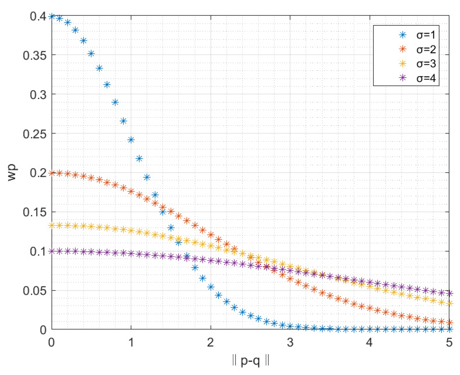
where is the two-dimensional vector coordinate of the central pixel and is the two-dimensional vector coordinate of the neighborhood pixel. is a Gaussian function, which can ensure the maximum weight of the central pixel. In addition, it can be seen from Figure 2 that compared with other values of , the pixels farther from the central pixel can be given lower weight and the pixels closer to the central pixel can be given higher weight when ; therefore, is set to a standard Gaussian function, in which is 0 and is 1.
For instance, the distances from the eight surrounding pixels to the target pixel are in order , , , , , , , and from left to right and from top to bottom in the negative x-direction mask, respectively; and the distances from the eight surrounding pixels to the target pixel are in order , , , , , , , and from left to right and from top to bottom in the bottom-right diagonal mask, respectively. Suppose variable denotes the distance between surrounding pixels and the target pixel in the 3 × 3 neighborhood. When is sorted in ascending order as , , , , and , we substitute into the function, and then the defined weights can be obtained by
If the 3 × 3 fractional differential masks in Table 1 are used in each pixel of the original image, the pixels with the coefficient of 0 will be ignored. To make full use of the correlation between pixels, we use the above spatial weight to improve the G-L mask. It should be noted that the pixel with a constant coefficient of 1 is the target pixel. We divide the coefficients unevenly on the pixels with the distance of a 1-unit pixel from the target pixel according to the weight, and divide the coefficients unevenly on the pixels with the distance of a 2-unit pixel from the target pixel according to the weight. Table 2 shows the G-L masks in negative x-direction, negative y-direction, and upper-right diagonal direction on the left, as well as the normalized spatial domain masks in the negative x-direction, negative y-direction, and upper-right diagonal direction on the right.
The 3 × 3 masks in eight directions (0°, 45°, 90°, 135°, 180°, 225°, 270°, and 315°) are obtained, and the 5 × 5 masks in eight directions are extended by the 3 × 3 masks with adding zero centered around the target pixel, and then the 5 × 5 masks in eight directions are stacked to obtain the new 5 × 5 mask, as illustrated in Table 3.
Moreover, we divide each item in the improved mask by the sum of all the coefficients to obtain the normalized mask. Finally, we use the spatial domain mask to filter the image and implement histogram equalization (HE) to enhance the contrast of the image with a small dynamic range.
where is the image after spatial domain fractional differential filtering, and is the enhanced image.
3.4.2. Intensity Domain Fractional Differential Model
Considering the difference in the similarity and brightness between the neighboring pixel and the center pixel, we modified the fractional-order differential coefficients by using the intensity domain weights. The difference between the center pixel value and the adjacent pixel value is relatively small, which indicates that the change of pixel values in this area is not obvious; that is, it is usually in a flat area. We need to give higher weights to the points whose grey values are closer to the grey values of the center point, thereby highlighting the textural details of the flat area. The difference between the center pixel value and adjacent pixel values is large, which indicates that the change of pixel values in this area is relatively obvious, and the area contains boundary information. We need to give lower weights to the points whose grey values are farther away from the center point so that the current pixel is less affected, which preserves the edge information. The grey distance weight formula is generated by the standard Gaussian function as follows:
where is the intensity value of the two-dimensional vector coordinate of the central pixel and is the intensity value of the two-dimensional vector coordinate of the pixel adjacent to the central pixel.
Therefore, the two-dimensional fractional differential expression can be written as follows:
The nonzero coefficients are in order as follows:
where represents the neighborhood that contains the th nonzero coefficient in the fractional differential mask, is the weight of pixel in , and is the sum of all coefficients in neighborhood .
The anisotropic filter is constructed according to (38) to obtain the intensity domain fractional differential mask, which is shown in Table 4.
After fractional differential filtering using the above mask, we use linear transformation and contrast limited adaptive histogram equalization (CLAHE) [42] to further enhance the global brightness and contrast of the image.
where K is the adjustment parameter, is the image after intensity domain fractional differential filtering, and is the final enhanced image. The above-enhanced image of the spatial domain fractional differential filter and the enhanced image of the intensity domain fractional differential filter are synthesized to obtain the bilateral fractional differential enhanced image.
After inverting the bilateral fractional differential image as (40), the final enhanced image can be obtained.
The above content is summarized, and the proposed multispectral image enhancement algorithm is described in the Algorithm 1.
| Algorithm 1. Multispectral image enhancement based on IDCP_BFD. | |
| Input: A original multispectral image of the test dataset. | |
Let be any bands in the multispectral image. | |
| |
| |
| end for ● Calculate the final enhanced image S by considering (40). Output: The enhanced result of the original image. | |
4. Experimental Results and Analysis
To verify the effectiveness of our proposed algorithm, we evaluate the visual effects and objective indicators of the algorithm. All experiments in the paper are performed on a personal computer with an Intel (R) Core (TM) i5-11300H 3.10 GHz CPU. Retinex-Net method uses Python 3.6 and other methods use MATLAB R2020b. Code is available at https://1drv.ms/u/s!ApVw-FZtwy2wfkXeeKpkh2HLvtY?e=YBgDiq (3 January 2022).
By referring to the relevant works of multispectral remote sensing image enhancement [30,31,32,33,34,35,36,37,38], five well-known evaluation indexes, including the contrast, image intensity, information entropy, average gradient, and execution time are used to evaluate the performance of different methods.
Contrast represents the difference scale in the brightness levels of the brightest area and the darkest area in an image. The greater the contrast is, the better the image quality; however, the smaller the contrast is, the less obvious the image change. Contrast is defined by
where C represents the image contrast. represents the intensity difference between adjacent pixels. indicates the distribution probability of the pixel with intensity difference.
The image intensity denotes the average value of an image.
where μ represents the image intensity, M, N represent the dimension of image, represents the intensity of the pixel .
Entropy reflects the information that an image carries.
where S represents the input image, and pk represents the proportion of pixels with gray value k in the image. The larger the information entropy, the richer the information of the image.
The average gradient represents the ability of an image to express minute details and textural changes.
where S(i,j) represents the intensity value of pixel coordinates of the image. Generally, the greater the average gradient is, the richer the image hierarchy and the clearer the image.
To confirm the performance of the proposed algorithm, we conducted experiments in three ways. In Section 4.3, we compare our bilateral fractional differential algorithm with five differential filtering algorithms, such as Sobel operator, Laplacian operator, the Yipufei approach [19], the MGL approach [20], the approach of Wadhwa et al. [21], on the premise of the proposed dark channel prior algorithm. The Yipufei approach and the MGL approach are set in the fixed fractional order as in this paper. The approach of Wadhwa et al. uses the adaptive fractional order; thus, the parameters are obtained from original literature. In Section 4.4, we compare our IDCP algorithm with the original DCP algorithm of 3-bands, IDCP algorithm of 3-bands, 4-bands, 5-bands, 6-bands, and 7-bands on the premise of the proposed BFD algorithm. In Section 4.5, we compare the proposed IDCP_BFD algorithm with the Retinex-Net approach [29], the LIME approach [43], and the ACSEA approach [44] to evaluate the overall algorithm. All parameters are obtained from the parameters set by each author.
4.1. Dataset
The Landsat-5 satellite is the fifth satellite in the Landsat series with an orbit altitude of 705 km, which was launched in March 1984. This is an Earth observation satellite that carries a thematic mapper (TM) and a multispectral scanner (MSS). To date, the images delivered by Landsat-5 satellites have been widely used in many fields and have provided a great deal of effective information worldwide. The Landsat-5 satellite is also the longest optical remote sensing satellite in orbit.
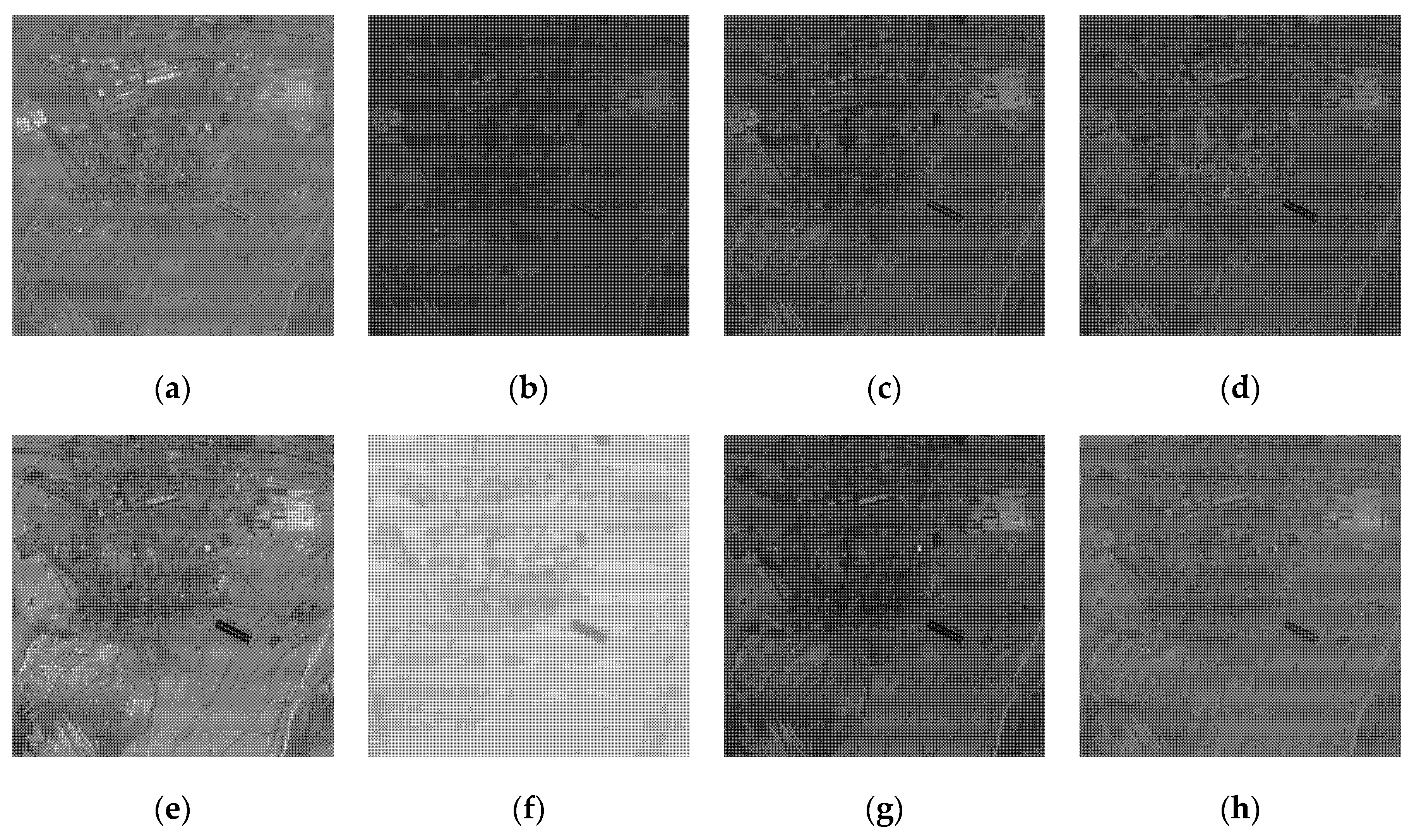
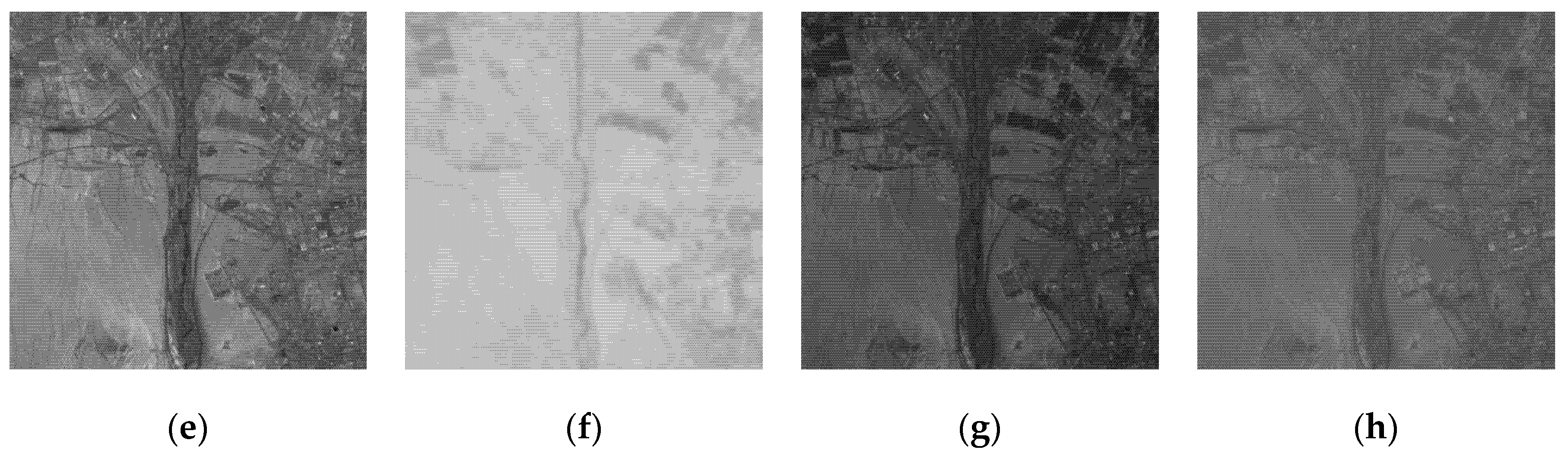
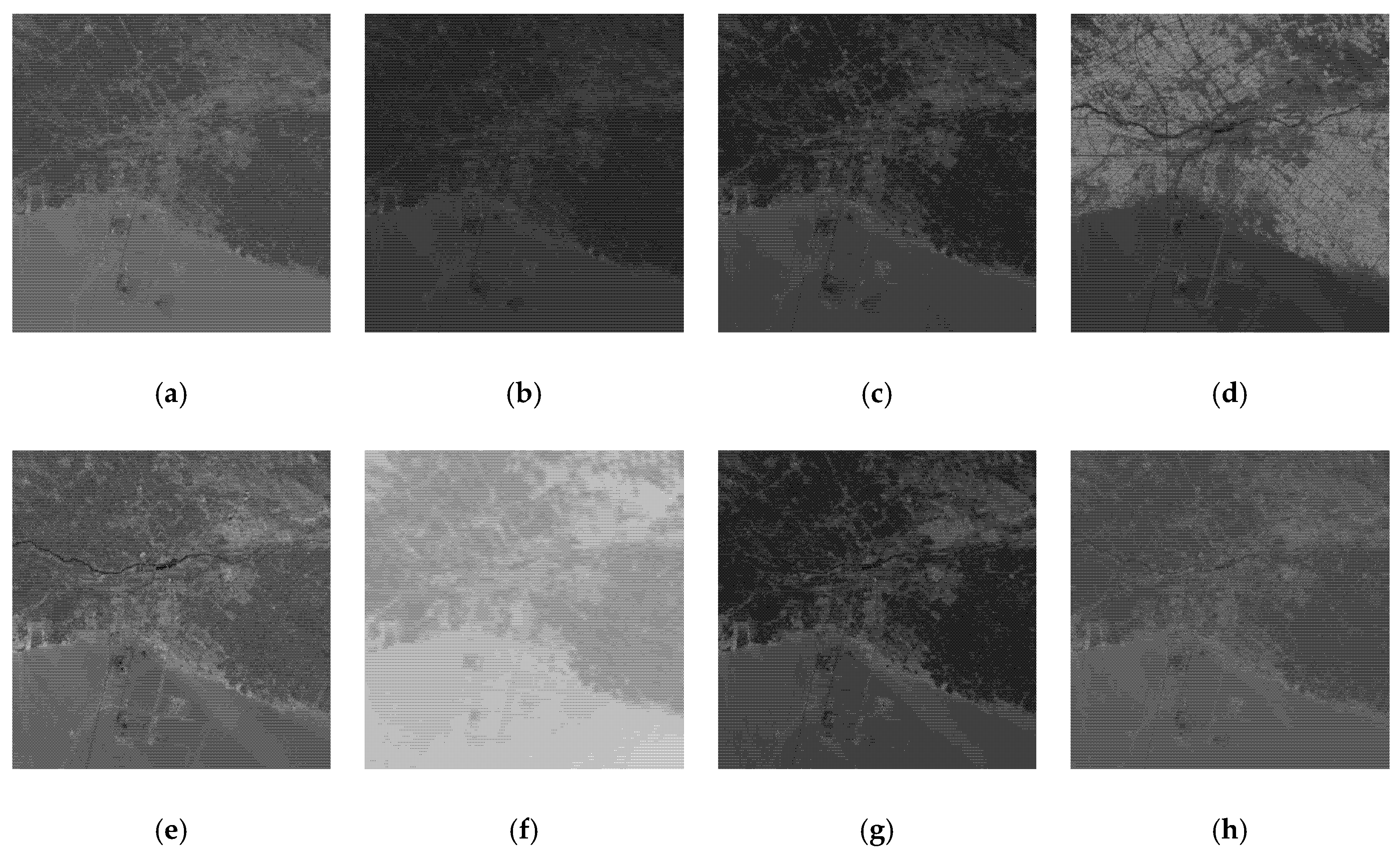
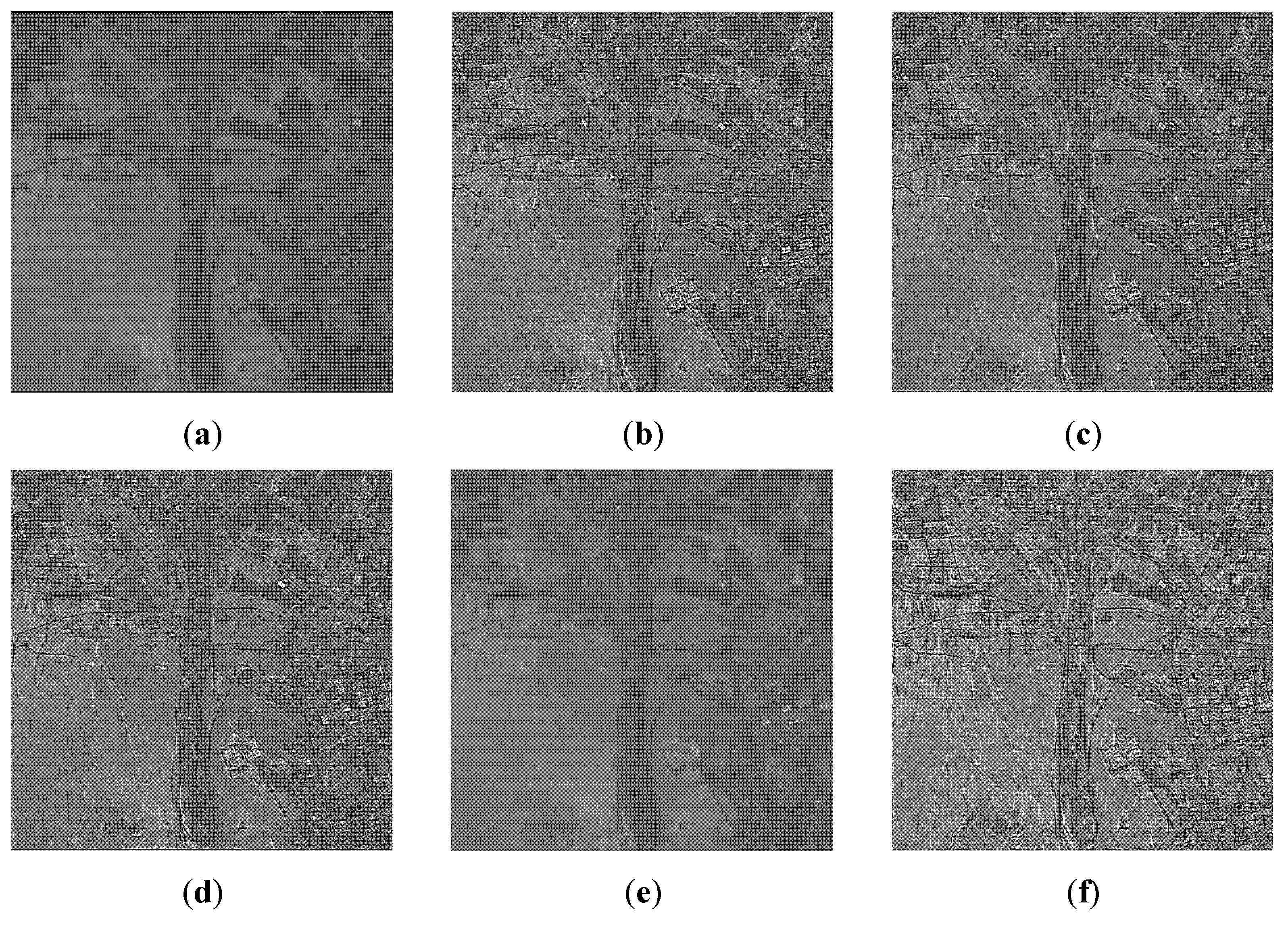
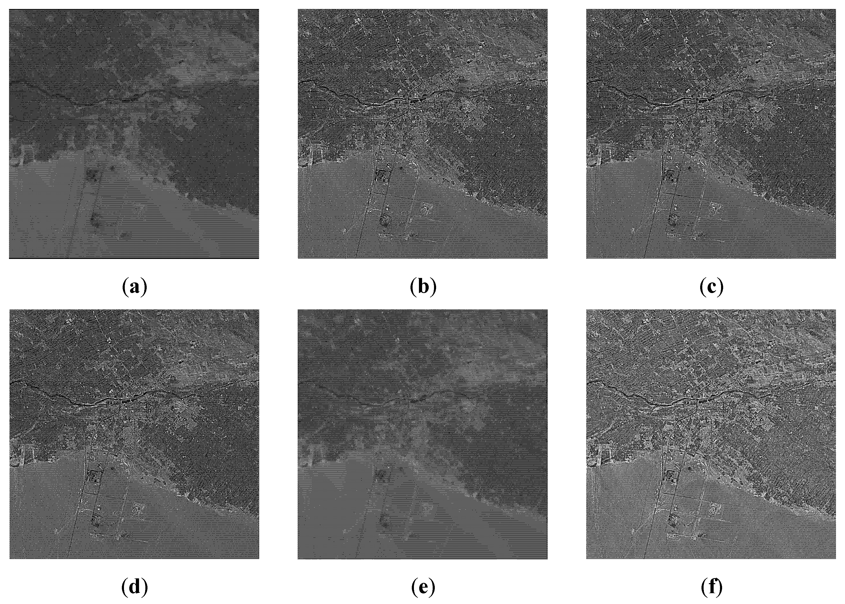
In this paper, we chose thirty multispectral remote sensing images from Changji, Xinjiang in 2011 and Turpan, Xinjiang in 2009 obtained by the Landsat-5 satellite and then produced the multispectral image dataset. Each image of the dataset contains 500 × 500 pixels. Landsat TM image contains 7 bands ranging from visible to thermal infrared wavelength. Band 1 is the blue band with a wavelength range from 0.45 μm to 0.52 μm and a spatial resolution of 30 m, which has strong penetration into water and can effectively distinguish soil and vegetation. Band 2 is the green band with a wavelength range from 0.52 μm to 0.60 μm and a spatial resolution of 30 m, which is relatively sensitive to the response of healthy and lush plants. Band 3 is the red band with a wavelength range from 0.63 μm to 0.69 μm and a spatial resolution of 30 m, which is the main band of chlorophyll absorption and is usually used to observe bare soil and vegetation. Band 4 is the near-infrared band with a wavelength range from 0.76 μm to 0.90 μm and a spatial resolution of 30 m, which is a general band for plants and is usually used for the analysis of crop growth. Band 5 is the shortwave infrared band with a wavelength range from 1.55 μm to 1.75 μm and a spatial resolution of 30 m, which is used to distinguish the characteristics of roads, bare soil, and water systems. Band 6 is the thermal infrared band with a wavelength range from 10.40 μm to 12.50 μm and a spatial resolution of 120 m, which is used to distinguish the characteristics of roads, bare soil, and water. Band 7 is the mid-infrared band with a wavelength range from 2.08 μm to 2.35 μm and a spatial resolution of 30 m, which is used to respond to targets emitting thermal radiation. Figure 3, Figure 4 and Figure 5 present three sub-sets of multispectral dataset. Each sub-set shows Band 1–7 and the composite image of 7 bands, in which the composite image represents the superposition of all bands in the original multispectral data and shows the overall visual effect of the unenhanced image. The multispectral remote sensing images reflect the ground information of different spectral bands in the same region. From Figure 4a, we can see that the characteristics of water bodies and urban colonies are obvious in band 1. Figure 4d and Figure 5d show that band 4 has relatively clear terrace characteristics. Figure 4e reflects the clear characteristics of urban settlements and roads in band 5. In Figure 3a, the ridge and other lithologic characteristics of band 7 are more prominent; therefore, we integrate seven bands to generate a single band image in the subsequent enhancement processing. Compared with the enhancement algorithm using only one band, the 7-bands combination algorithm can make better use of the detailed information of different bands, restore the real and rich features of ground objects, and then improve the visual interpretation effect.
4.2. Parameter Analysis
In this part, we discuss the parameters in the paper. In the proposed algorithm, some free parameters need to be adjusted in advance, including K and v. We carry out two sets of experiments to verify the impact of these parameters on the performance of the algorithm.
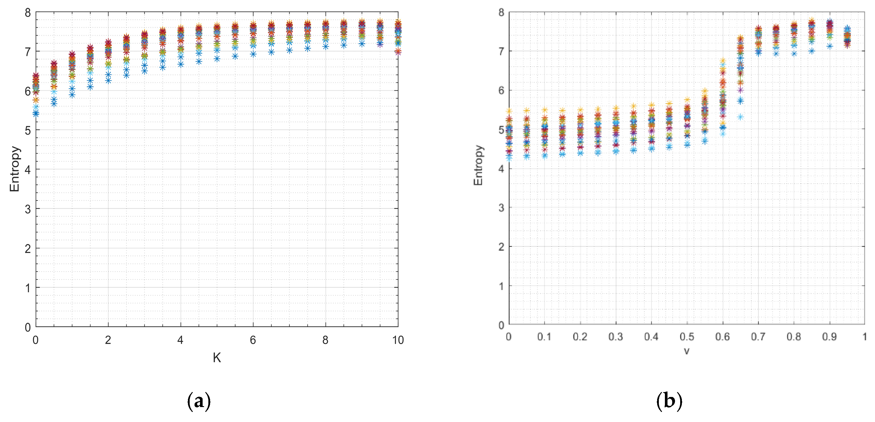
The introduction of is to control the degree of brightness adjustment. The fractional filtering in the intensity domain makes the overall brightness of the image lower; therefore, is used to constrain the linear transformation and improve the brightness value of multiband images. For this reason, we vary from 0 to 10 with 0.5 intervals and test on multispectral image datasets, including 30 images. The influence of on image information is given in Figure 6a. From Figure 6a, we can see that with the increase of , the information entropy gradually increases and tends to be stable. To the end, is set to 6 to retain the image information abundance in this paper.
In addition, we need to set the order of the fractional differential algorithm. As for our fractional differential framework, the importance of neighborhood points changes with the order. If the order is too small and the target pixel is not prominent enough, the gray value of the image edge may mutate, resulting in the local region being too bright or too dark. If the order is too large, the gray value of the image may be too large or too small to exceed the gray display range. We vary the order from 0 to 1 with 0.05 interval and test on multispectral image datasets including 30 images. From Figure 6b, we can see that the information entropy increases with the value of order but decreases sharply when is close to 1, which has been mentioned in Luo’s work [45]; therefore, we set to 0.8 to ensure the enhancement effects.
4.3. Comparative Experiments of Other Methods Based on Differential Filtering
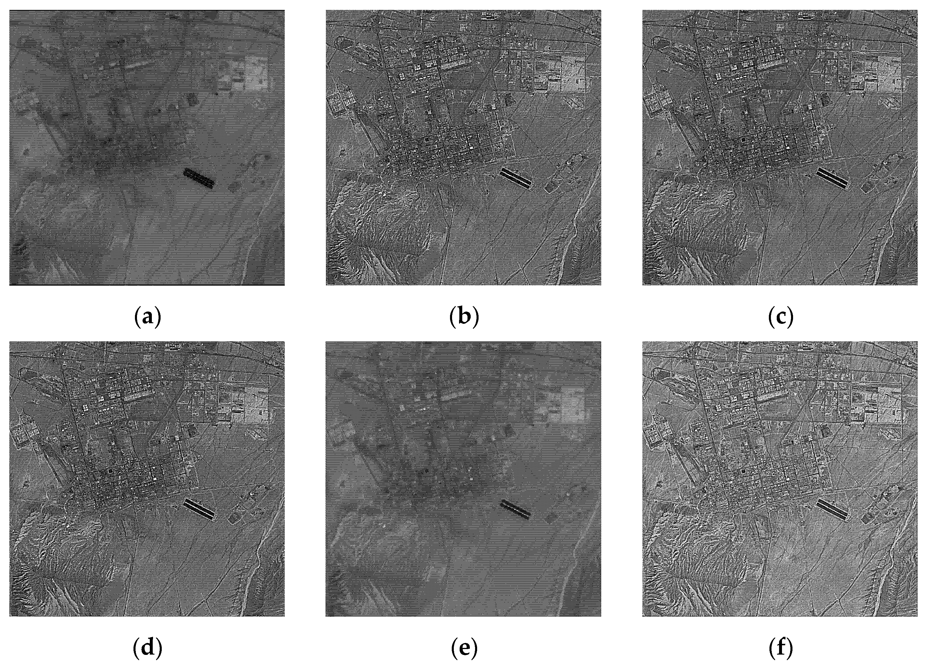
In this part, we compared the proposed BFD algorithm with the image enhancement methods based on differential filtering, such as Sobel operator, Laplacian operator, Yipufei approach [19], MGL approach [20], and the approach of Wadhwa et al. [21]. The enhanced visual effects of test images are shown in Figure 7, Figure 8 and Figure 9. The ground objects of the original images are different in each band; that is, the same ground objects are clear in some bands and blurred in the other bands. By synthesizing the dimensional information, the enhanced image with more complete features can be obtained. Figure 3, Figure 4 and Figure 5 and Figure 7, Figure 8 and Figure 9 show that most of the enhanced images can improve the clarity and texture details of the original image to some extent. Comparing Figure 3a,e, Figure 4a,e and Figure 5a,e with Figure 7a,e, Figure 8a,e and Figure 9a,e, we can see that although the contrasts of the images using the Sobel method and the approach of Wadhwa et al. [21] are higher than that of the original image, the brightness adjustment effects are not obvious, and the processed images still have fuzzy edge features. Figure 7b–d, Figure 8b–d and Figure 9b–d show that the results generated by the Laplacian algorithm, the Yipufei algorithm [19], and the MGL approach [20] can enhance the edge and textural area of the original images to a certain extent, but the overall visual effects of the images are generally dark, and the image contrast is not effectively improved. Furthermore, Figure 9c,d show that the Yipufei algorithm [19] and the MGL approach [20] do not recover some details of dark areas. The proposed method shows good visual effects on three sets of images, as shown in Figure 7f, Figure 8f and Figure 9f. It is evident from the enhanced images that our fractional differential method performs exceedingly well in maintaining the details. Simultaneously, our method can fully enhance the edge and textural details and improve the contrast and brightness of multispectral images.
Table 5 shows the quantitative results of each band from Figure 3, Figure 4 and Figure 5 and the average quantitative results of 30 original multispectral images. Table 6 shows the quantitative results of six differential methods used in Figure 7, Figure 8 and Figure 9 and the average quantitative results of the comparison methods used in 30 multispectral images. As shown in Table 5, band 6 has relatively high brightness values, and less information, and band 5 has relatively high information entropy and average gradient; however, as a whole, the original multispectral images have low contrast and weak edge retention. By comparing the data in Table 5 and Table 6, it can be observed that the proposed BFD method can effectively improve these problems of the original images. The enhanced images using the BFD method have a relatively higher information entropy and average gradient than each band of original multispectral images, especially band 5 with the best comprehensive index, which reflects that the enhanced images contain richer information, clearer edge textural features, and higher ability to maintain details. In addition, it can be seen that the proposed method effectively improves the global contrast, thereby enhancing the visibility of the original multispectral images; therefore, the enhanced images have relatively moderate brightness value, clear edge, and rich details, which can improve the basic features of the original multispectral image.
Table 6 shows that the method proposed in this paper has a higher mean value and contrast than other differential algorithms, which shows that the enhanced image has good global visual quality. Moreover, the proposed method achieves the highest entropy and average gradient. This implies that our method can retain the advantages existing in the original image and highlight the local detail features. Furthermore, the running time of the proposed algorithm is higher than the other methods, apart from the approach of Wadhwa et al. [21]. This is because our bilateral fractional filtering algorithm needs to calculate the pixel difference in the neighborhood of an image, which makes the time consumption of the algorithm longer. Although the time of the BFD algorithm is long, the other four indexes of our method are higher than those of the five comparison methods; therefore, our algorithm is a better algorithm to meet the needs of human vision.
4.4. Comparative Experiments Based on Dark Channel Prior
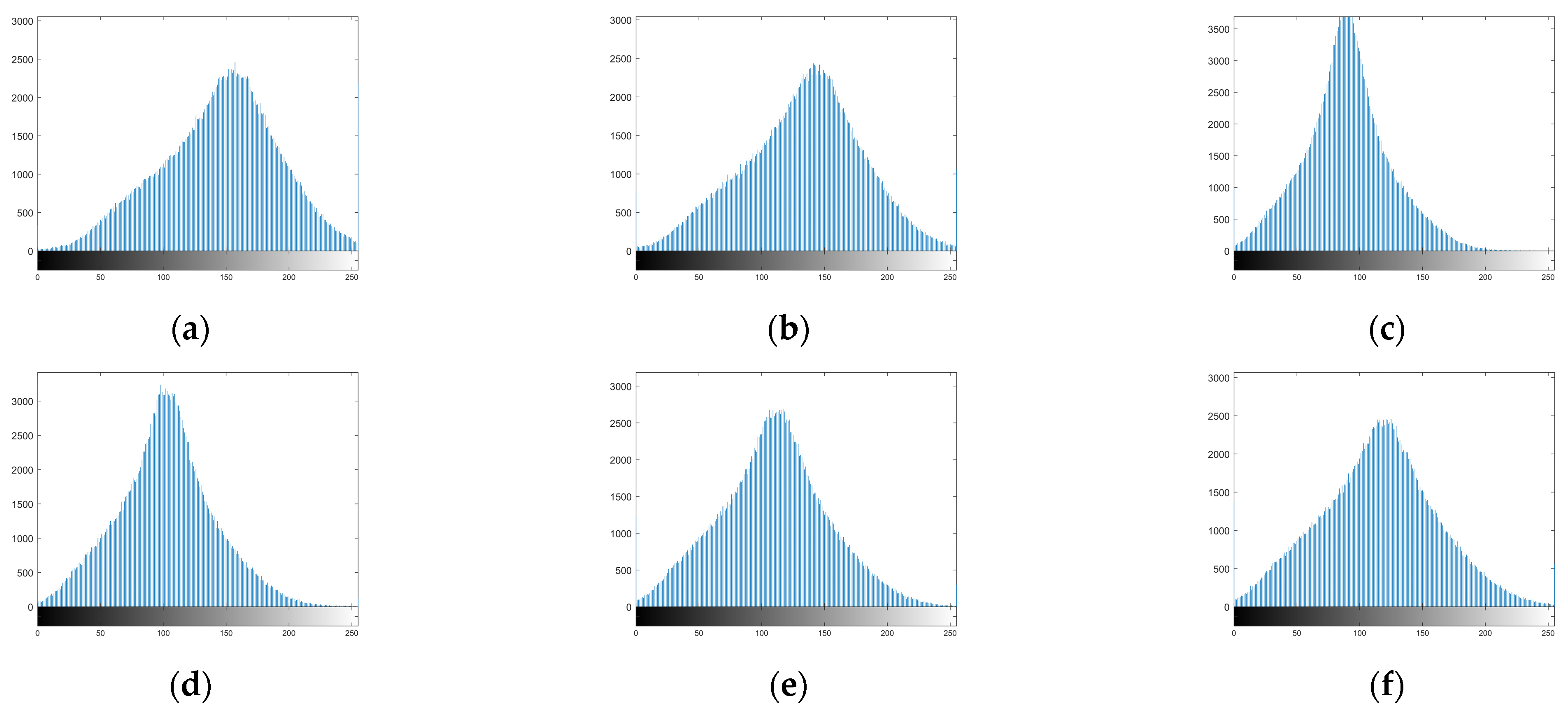
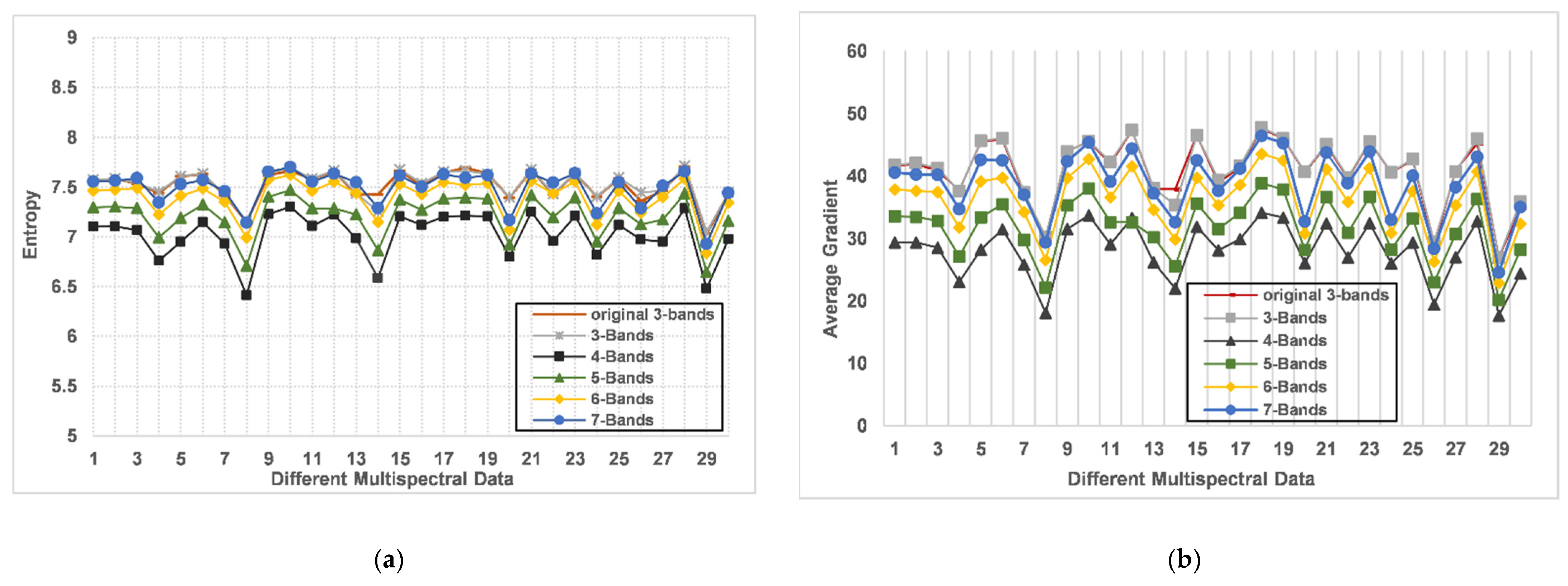
In this paper, we extend and improve the original dark channel algorithm; therefore, we have further experimented and discussed the dark channel algorithm in different bands. According to the average values of normalized information entropy and normalized image intensity, we rank the seven bands in descending order: Band 5, Band 6, Band 4, Band 7, Band 1, Band 3, and Band 2. Then we combine the above bands, including the first three bands, the first four bands, the first five bands, the first six bands, and the first seven bands. The original DCP algorithm is used to test 3-bands combinations and the proposed IDCP algorithm is used to test all band combinations. The experimental results are given in Figure 10 and Figure 11. It is readily observed that the histogram of Figure 10e can make full use of the whole dynamic range than the histograms of Figure 10b,c. This shows that the 7-bands algorithm used in this paper can obtain more detailed information. In addition, compared with Figure 10a,b, Figure 10e is closer to the normal distribution, and therefore closer to the ideal enhanced image [46]. Moreover, Figure 11 shows the information entropy and average gradient obtained by applying the DCP algorithm of 3-bands and the IDCP algorithm from 3-bands to 7-bands in the multispectral dataset. As shown in Figure 11a, the 7-bands algorithm has relatively higher information entropy, indicating that the proposed algorithm can maintain the image information and enhance the clarity of the images. From Figure 11b, it is clear that the average gradient of the 7-bands combined algorithm is relatively high, which shows that the image contains more detailed information. Theoretically, multispectral images exist “same body with different spectrum” phenomenon; that is, the same type of ground objects have different gray values in different bands; therefore, different electromagnetic wavebands can reflect different features. The 7-bands algorithm can use the spectrum information of all bands. On the whole, the 7-bands IDCP algorithm can better integrate information and improve image quality.
4.5. Comparative Experiments of Other Methods Based on Image Enhancement
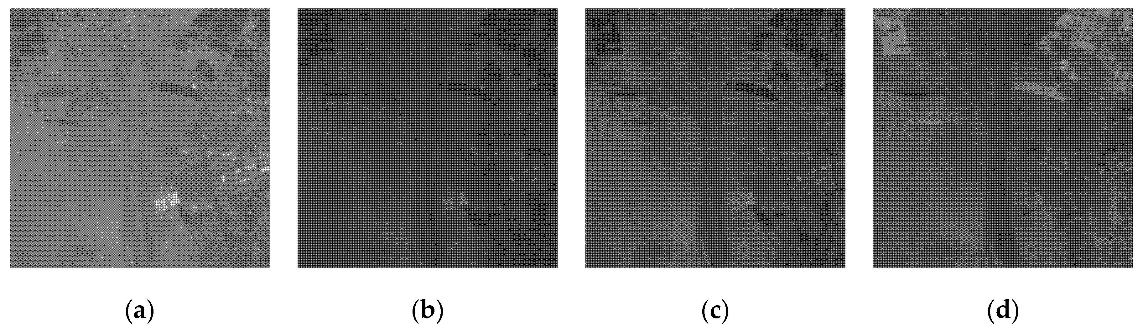
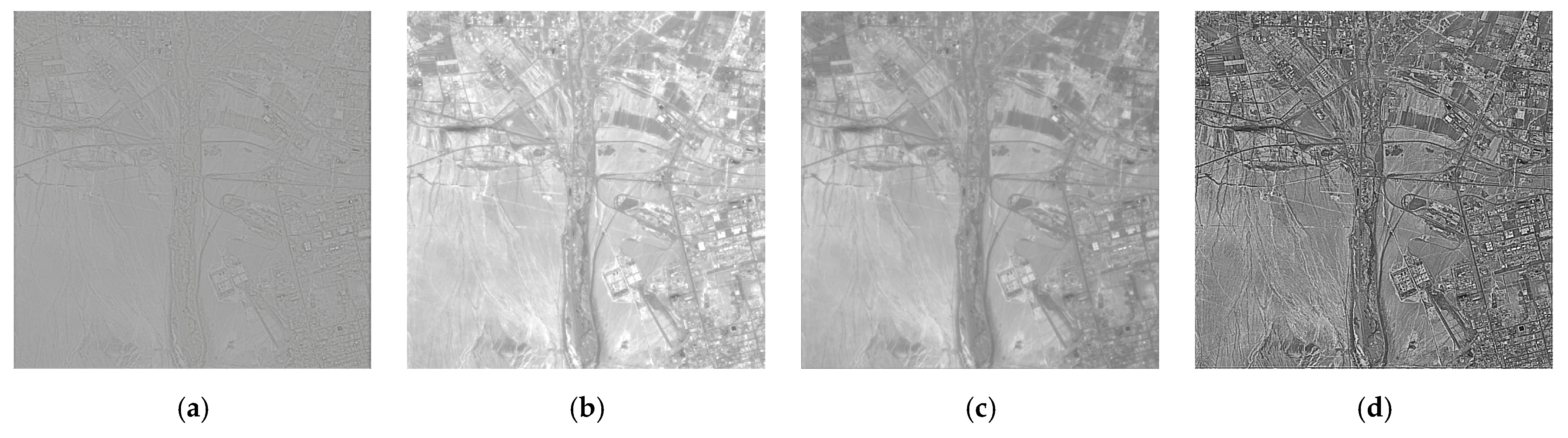
We compared the lasting image enhancement methods with our whole algorithm, such as the Retinex-Net approach, the LIME approach, and the ACSEA approach, which as shown in Figure 12 and Table 7. As shown in Figure 12a,b, the Retinex-Net approach and the LIME approach make the overall image brighter, but the sharpness is relatively lower. There are low contrast and loss of detail in the Retinex-Net approach, while saturation artifacts appear in the LIME approach. This is because the above methods are mainly used for low illumination image enhancement. Although they greatly improve the image brightness, they cannot preserve the edge details of the image well. In addition, Figure 12c shows that the ACSEA approach has uniform brightness but has relatively blurred texture details. As shown in Figure 12d, the proposed image enhancement method provides clearer edge details and texture features effectively.
Table 7 shows that the proposed IDCP_BFD has improved results in terms of contrast, entropy and average gradient than the other comparison algorithms; therefore, the enhanced image of the proposed algorithm has more texture details and can significantly highlight urban settlements, roads, and other ground features. It is clear that the proposed method is superior to other algorithms in maintaining the overall image quality.
5. Discussion
Due to the influence of sensors, atmospheric environment, and weather, multispectral remote sensing images usually have some problems such as distortion, blur, low contrast, and loss of details, which brings difficulties to the visual interpretation. From the above experiments, it can be seen that the proposed algorithm can effectively improve the image quality and clearly express the ground features. At the same time, the superiority of the proposed IDCP_BFD algorithm is also shown in the objective evaluation. The results mainly depend on the combination of bilateral fractional differential algorithm and improved dark channel prior algorithm. In particular, the BFD algorithm plays an important role in image texture detail and visual quality improvement. In this paper, we mainly implement the comparison methods in the Landsat-5 TM dataset. The proposed algorithm can still be used for other multispectral remote sensing datasets; however, the free parameters may change. Especially for datasets with a high overall brightness value, the brightness adjustment parameter can be appropriately reduced. In addition, the execution time of the proposed method is relatively long and the processing rate needs to be improved. In the future, we will further optimize the algorithm to achieve a higher image processing rate and try to use parameter adaptation to improve the robustness of the algorithm.
6. Conclusions
In this paper, a multispectral image enhancement method based on dark channel prior technology and the fractional differential algorithm is proposed. In this method, we extend the dark channel model from the RGB channel to multiple channels and use the spatial fractional differential algorithm to improve the guided filtering and optimize the transmittance estimation. Furthermore, we redistribute the coefficients defined by the G-L function according to the weights of the spatial domain and intensity domain and then use the improved fractional differential algorithm to obtain an enhanced image with a clearer edge and textural details. We perform experiments on the multispectral image dataset and compare the enhancement results of different algorithms qualitatively and quantitatively. Compared with other methods, the proposed method not only improves the global brightness and local contrast of the original multispectral image but also effectively enhances the edges and textural details of the image.
Author Contributions
Z.J. and W.C. conceived and designed the study; W.C. conducted the experiments and wrote the article; J.Y. and N.K.K. assisted by reviewing the article and providing editorial supervision. All authors have read and agreed to the published version of the manuscript.
Funding
This work was supported by the National Science Foundation of China (No. U1803261) and the International Science and Technology Cooperation Project of the Ministry of Education of the People’s Republic of China (No. 2016–2196).
Institutional Review Board Statement
Not applicable.
Informed Consent Statement
Not applicable.
Data Availability Statement
The data is obtained from the following: https://1drv.ms/u/s!ApVw-FZtwy2wfkXeeKpkh2HLvtY?e=YBgDiq (2 January 2022).
Conflicts of Interest
The authors declare no conflict of interest.
References
- Fu, X.; Wang, J.; Zeng, D.; Huang, Y.; Ding, X. Remote Sensing Image Enhancement Using Regularized-Histogram Equalization and DCT. IEEE Geosci. Remote Sens. Lett. 2015, 12, 2301–2305. [Google Scholar] [CrossRef]
- Lu, X.; Li, X. Multiresolution Imaging. IEEE Trans. Cybern. 2014, 44, 149–160. [Google Scholar] [CrossRef] [PubMed]
- Lu, X.; Wang, Y.; Yuan, Y. Graph-Regularized Low-Rank Representation for Destriping of Hyperspectral Images. IEEE Trans. Geosci. Remote Sens. 2013, 51, 4009–4018. [Google Scholar] [CrossRef]
- Wang, J.; Yang, Y.; Chen, Y.; Han, Y. LighterGAN: An Illumination Enhancement Method for Urban UAV Imagery. Remote Sens. 2021, 13, 1371. [Google Scholar] [CrossRef]
- Hagag, A.; Hassan, E.S.; Amin, M.; Abd El-Samie, F.E.; Fan, X. Satellite multispectral image compression based on removing sub-bands. Optik 2017, 131, 1023–1035. [Google Scholar] [CrossRef]
- Iqbal, M.Z.; Ghafoor, A.; Siddiqui, A.M. Satellite Image Resolution Enhancement Using Dual-Tree Complex Wavelet Transform and Nonlocal Means. IEEE Geosci. Remote Sens. Lett. 2013, 10, 451–455. [Google Scholar] [CrossRef]
- Lee, E.; Kim, S.; Kang, W.; Seo, D.; Paik, J. Contrast Enhancement Using Dominant Brightness Level Analysis and Adaptive Intensity Transformation for Remote Sensing Images. IEEE Geosci. Remote Sens. Lett. 2013, 10, 62–66. [Google Scholar] [CrossRef]
- Pyka, K. Wavelet-Based Local Contrast Enhancement for Satellite, Aerial and Close Range Images. Remote Sens. 2017, 9, 25. [Google Scholar] [CrossRef] [Green Version]
- Lisani, J.; Michel, J.; Morel, J.; Petro, A.B.; Sbert, C. An Inquiry on Contrast Enhancement Methods for Satellite Images. IEEE Trans. Geosci. Remote Sens. 2016, 54, 7044–7054. [Google Scholar] [CrossRef]
- Liu, J.; Zhou, C.; Chen, P.; Kang, C. An Efficient Contrast Enhancement Method for Remote Sensing Images. IEEE Geosci. Remote Sens. Lett. 2017, 14, 1715–1719. [Google Scholar] [CrossRef]
- Liu, C.; Sui, X.; Kuang, X.; Liu, Y.; Gu, G.; Chen, Q. Optimized Contrast Enhancement for Infrared Images Based on Global and Local Histogram Specification. Remote Sens. 2019, 11, 849. [Google Scholar] [CrossRef] [Green Version]
- Febin, I.P.; Jidesh, P.; Bini, A.A. A Retinex-Based Variational Model for Enhancement and Restoration of Low-Contrast Remote-Sensed Images Corrupted by Shot Noise. IEEE J. Sel. Top. Appl. Earth Obs. Remote Sens. 2020, 13, 941–949. [Google Scholar] [CrossRef]
- Jang, J.H.; Kim, S.D.; Ra, J.B. Enhancement of Optical Remote Sensing Images by Subband-Decomposed Multiscale Retinex With Hybrid Intensity Transfer Function. IEEE Geosci. Remote Sens. Lett. 2011, 8, 983–987. [Google Scholar] [CrossRef]
- Ye, X.; Yang, H.; Li, C.; Jia, Y.; Li, P. A Gray Scale Correction Method for Side-Scan Sonar Images Based on Retinex. Remote Sens. 2019, 11, 1281. [Google Scholar] [CrossRef] [Green Version]
- Song, M.; Qu, H.; Zhang, G.; Tao, S.; Jin, G. A Variational Model for Sea Image Enhancement. Remote Sens. 2018, 10, 1313. [Google Scholar] [CrossRef] [Green Version]
- Chaudhuri, D.; Kushwaha, N.K.; Samal, A. Semi-Automated Road Detection From High Resolution Satellite Images by Directional Morphological Enhancement and Segmentation Techniques. IEEE J. Sel. Top. Appl. Earth Obs. Remote Sens. 2012, 5, 1538–1544. [Google Scholar] [CrossRef]
- Bandeira, A. Random Laplacian Matrices and Convex Relaxations. Found. Comput. Math. 2015, 18, 345–379. [Google Scholar] [CrossRef] [Green Version]
- Chen, S.; Zhao, F. The Adaptive Fractional Order Differential Model for Image Enhancement Based on Segmentation. Int. J. Pattern Recognit. Artif. Intell. 2018, 32, 1854005. [Google Scholar] [CrossRef]
- Pu, Y.; Zhou, J.; Yuan, X. Fractional Differential Mask: A Fractional Differential-Based Approach for Multiscale Texture Enhancement. IEEE Trans. Image Processing 2010, 19, 491–511. [Google Scholar] [CrossRef]
- Hemalatha, S.; Margret Anouncia, S. G-L fractional differential operator modified using auto-correlation function: Texture enhancement in images. Ain Shams Eng. J. 2018, 9, 1689–1704. [Google Scholar] [CrossRef]
- Wadhwa, A.; Bhardwaj, A. Enhancement of MRI images of brain tumor using Grünwald Letnikov fractional differential mask. Multimed. Tools Appl. 2020, 79, 25379–25402. [Google Scholar] [CrossRef]
- He, K.; Sun, J.; Tang, X. Single Image Haze Removal Using Dark Channel Prior. IEEE Trans. Pattern Anal. Mach. Intell. 2011, 33, 2341–2353. [Google Scholar] [CrossRef] [PubMed]
- Xuan, D.; Guan, W.; Yi, P.; Weixin, L.; Jiangtao, W.; Wei, M.; Yao, L. Fast efficient algorithm for enhancement of low lighting video. In Proceedings of the 2011 IEEE International Conference on Multimedia and Expo, Barcelona, Spain, 11–15 July 2011; pp. 1–6. [Google Scholar]
- Caballero, R.; Berbey-Alvarez, A. Underwater Image Enhancement Using Dark Channel Prior and Image Opacity. In Proceedings of the 2019 7th International Engineering, Sciences and Technology Conference (IESTEC), Panama City, Panama, 9–11 October 2019; pp. 556–561. [Google Scholar]
- Im, J.; Yoon, I.; Hayes, M.H.; Paik, J. Dark channel prior-based spatially adaptive contrast enhancement for back lighting compensation. In Proceedings of the 2013 IEEE International Conference on Acoustics, Speech and Signal Processing, Vancouver, BC, Canada, 26–31 May 2013; pp. 2464–2468. [Google Scholar]
- Sonkar, P.K.; Raj, K. Single Image Dehazing Using Dark Channel Prior With Median Filter and Contrast Enhancement. In Proceedings of the 2020 IEEE International Conference for Innovation in Technology (INOCON), Bangluru, India, 6–8 November 2020; pp. 1–6. [Google Scholar]
- Yang, H.; Chen, P.; Huang, C.; Zhuang, Y.; Shiau, Y. Low Complexity Underwater Image Enhancement Based on Dark Channel Prior. In Proceedings of the 2011 Second International Conference on Innovations in Bio-inspired Computing and Applications, Shenzhen, China, 16–18 December 2011; pp. 17–20. [Google Scholar]
- Yang, H.; Wang, J. Color image contrast enhancement by co-occurrence histogram equalization and dark channel prior. In Proceedings of the 2010 3rd International Congress on Image and Signal Processing, Yantai, China, 16–18 October 2010; pp. 659–663. [Google Scholar]
- Wei, C.; Wang, W.; Yang, W.; Liu, J. Deep Retinex Decomposition for Low-Light Enhancement. arXiv 2018, arXiv:1808.04560v1. [Google Scholar]
- Tian, L.; Du, Q.; Younan, N.; Kopriva, I. Multispectral image enhancement with extended offset-sparsity decomposition. In Proceedings of the 2016 IEEE International Geoscience and Remote Sensing Symposium (IGARSS), Beijing, China, 10–15 July 2016; pp. 4383–4386. [Google Scholar]
- Bhandari, A.K.; Gadde, M.; Kumar, A.; Singh, G.K. Comparative analysis of different wavelet filters for low contrast and brightness enhancement of multispectral remote sensing images. In Proceedings of the 2012 International Conference on Machine Vision and Image Processing (MVIP), Coimbatore, India, 14–15 December 2012; pp. 81–86. [Google Scholar]
- Bhandari, A.K.; Kumar, A.; Singh, G.K. SVD Based Poor Contrast Improvement of Blurred Multispectral Remote Sensing Satellite Images. In Proceedings of the 2012 Third International Conference on Computer and Communication Technology, Allahabad, India, 23–25 November 2012; pp. 156–159. [Google Scholar]
- Suresh, S.; Das, D.; Lal, S. A Framework for Quality Enhancement of Multispectral Remote Sensing Images. In Proceedings of the 2017 Ninth International Conference on Advanced Computing (ICoAC), Chennai, India, 14–16 December 2017; pp. 9–14. [Google Scholar]
- Wang, M.; Zheng, X.; Feng, C. Color constancy enhancement for multi-spectral remote sensing images. In Proceedings of the 2013 IEEE International Geoscience and Remote Sensing Symposium—IGARSS, Melbourne, VIC, Australia, 21–26 July 2013; pp. 864–867. [Google Scholar]
- Lu, S.-l.; Zou, L.-j.; Shen, X.-h.; Wu, W.-y.; Zhang, W. Multi-spectral remote sensing image enhancement method based on PCA and IHS transformations. J. Zhejiang Univ. SCIENCE A 2011, 12, 453–460. [Google Scholar] [CrossRef]
- Venkatakrishnamoorthy, T.; Reddy, G.U. Cloud enhancement of NOAA multispectral images by using independent component analysis and principal component analysis for sustainable systems. Comput. Electr. Eng. 2019, 74, 35–46. [Google Scholar] [CrossRef]
- Mulla, A.; Baviskar, J.; Mohhamed, R.; Baviskar, A. Adaptive Band Specific Image Enhancement Scheme for Segmented Satellite Images. In Proceedings of the 2015 International Conference on Pervasive Computing (ICPC), Pune, India, 8–10 January 2015; pp. 1–5. [Google Scholar]
- Yang, C.; Lu, L.; Lin, H.; Guan, R.; Shi, X.; Liang, Y. A Fuzzy-Statistics-Based Principal Component Analysis (FS-PCA) Method for Multispectral Image Enhancement and Display. IEEE Trans. Geosci. Remote Sens. 2008, 46, 3937–3947. [Google Scholar] [CrossRef]
- Cafagna, D. Fractional calculus: A mathematical tool from the past for present engineers [Past and present]. IEEE Ind. Electron. Mag. 2007, 1, 35–40. [Google Scholar] [CrossRef]
- Matlob, M.A.; Jamali, Y. The Concepts and Applications of Fractional Order Differential Calculus in Modelling of Viscoelastic Systems: A primer. Crit. Rev. Biomed. Eng. 2017, 47, 249–276. [Google Scholar] [CrossRef]
- Che, J.; Shi, Y.; Xiang, Y.; Ma, Y. The fractional differential enhancement of image texture features and its parallel processing optimization. In Proceedings of the 2012 5th International Congress on Image and Signal Processing, Chongqing, China, 16–18 October 2012; pp. 330–333. [Google Scholar]
- Zuiderveld, K. Contrast Limited Adaptive Histogram Equalization. In Graphics Gems; Heckbert, P.S., Ed.; Academic Press: San Diego, CA, USA, 1994; pp. 474–485. [Google Scholar]
- Guo, X.; Li, Y.; Ling, H. LIME: Low-Light Image Enhancement via Illumination Map Estimation. IEEE Trans. Image Processing 2017, 26, 982–993. [Google Scholar] [CrossRef]
- Suresh, S.; Lal, S.; Reddy, C.S.; Kiran, M.S. A Novel Adaptive Cuckoo Search Algorithm for Contrast Enhancement of Satellite Images. IEEE J. Sel. Top. Appl. Earth Obs. Remote Sens. 2017, 10, 3665–3676. [Google Scholar] [CrossRef]
- Luo, X.; Zeng, T.; Zeng, W.; Huang, J. Comparative analysis on landsat image enhancement using fractional and integral differential operators. Computing 2020, 102, 247–261. [Google Scholar] [CrossRef]
- Demirel, H.; Ozcinar, C.; Anbarjafari, G. Satellite Image Contrast Enhancement Using Discrete Wavelet Transform and Singular Value Decomposition. IEEE Geosci. Remote Sens. Lett. 2010, 7, 333–337. [Google Scholar] [CrossRef]
Figure 1.
Algorithm flow chart.

Figure 2.
The effect of different spatial distance |||| on weight .

Figure 3.
Original multispectral data 1: (a) Band 1; (b) Band 2; (c) Band 3; (d) Band 4; (e) Band 5; (f) Band 6; (g) Band 7; (h) 7-bands composite image.
Figure 3.
Original multispectral data 1: (a) Band 1; (b) Band 2; (c) Band 3; (d) Band 4; (e) Band 5; (f) Band 6; (g) Band 7; (h) 7-bands composite image.

Figure 4.
Original multispectral data 2: (a) Band 1; (b) Band 2; (c) Band 3; (d) Band 4; (e) Band 5; (f) Band 6; (g) Band 7; (h) 7-bands composite image.
Figure 4.
Original multispectral data 2: (a) Band 1; (b) Band 2; (c) Band 3; (d) Band 4; (e) Band 5; (f) Band 6; (g) Band 7; (h) 7-bands composite image.


Figure 5.
Original multispectral data 3: (a) Band 1; (b) Band 2; (c) Band 3; (d) Band 4; (e) Band 5; (f) Band 6; (g) Band 7; (h) 7-bands composite image.
Figure 5.
Original multispectral data 3: (a) Band 1; (b) Band 2; (c) Band 3; (d) Band 4; (e) Band 5; (f) Band 6; (g) Band 7; (h) 7-bands composite image.

Figure 6.
Information entropy with different parameters in the multispectral image dataset: (a) brightness adjustment parameter ; (b) fractional differential order .
Figure 6.
Information entropy with different parameters in the multispectral image dataset: (a) brightness adjustment parameter ; (b) fractional differential order .

Figure 7.
Enhanced image of data 1 by using our IDCP algorithm with: (a) Sobel; (b) Laplacian; (c) Yipufei [19]; (d) MGL [20]; (e) Wadhwa et al. [21]; (f) Proposed BFD.

Figure 8.
Enhanced image of data 2 by using our IDCP algorithm with: (a) Sobel; (b) Laplacian; (c) Yipufei [19]; (d) MGL [20]; (e) Wadhwa et al. [21]; (f) Proposed BFD.

Figure 9.
Enhanced image of data 3 by using our IDCP algorithm with: (a) Sobel; (b) Laplacian; (c) Yipufei [19]; (d) MGL [20]; (e) Wadhwa et al. [21]; (f) Proposed BFD.

Figure 10.
The histograms corresponding to enhanced data 1 by using different input bands combinations: (a) original DCP of 3-Bands; (b) IDCP of 3-Bands; (c) IDCP of 4-Bands; (d) IDCP of 5-Bands; (e) IDCP of 6-Bands; (f) IDCP of 7-Bands.
Figure 10.
The histograms corresponding to enhanced data 1 by using different input bands combinations: (a) original DCP of 3-Bands; (b) IDCP of 3-Bands; (c) IDCP of 4-Bands; (d) IDCP of 5-Bands; (e) IDCP of 6-Bands; (f) IDCP of 7-Bands.

Figure 11.
The quantitative results of different input bands combinations used in 30 multispectral data: (a) entropy; (b) average gradient.
Figure 11.
The quantitative results of different input bands combinations used in 30 multispectral data: (a) entropy; (b) average gradient.

Figure 12.
Enhanced image of data 2 by using: (a) Retinex-Net; (b) LIME; (c) ACSEA; (d) Proposed IDCP_BFD.
Figure 12.
Enhanced image of data 2 by using: (a) Retinex-Net; (b) LIME; (c) ACSEA; (d) Proposed IDCP_BFD.


Table 1.
G-L fractional differential mask.
Table 2.
The 3 × 3 G-L fractional differential masks and 3 × 3 spatial domain fractional differential masks in (A) negative x-direction; (B) negative y-direction; (C) upper-right diagonal direction.
Table 2.
The 3 × 3 G-L fractional differential masks and 3 × 3 spatial domain fractional differential masks in (A) negative x-direction; (B) negative y-direction; (C) upper-right diagonal direction.
| (A) | |||||
| (B) | |||||
| (C) | |||||
Table 3.
The 5 × 5 spatial domain fractional differential mask.
Table 4.
Intensity domain fractional differential mask.
Table 5.
The quantitative results of the original multispectral data.
| Original Images | Metrics | ||||
|---|---|---|---|---|---|
| μ | C | H | AG | ||
| Data 1 | Band1 | 113.73 | 50.06 | 5.54 | 4.33 |
| Band2 | 59.25 | 21.06 | 5.06 | 2.91 | |
| Band3 | 71.15 | 44.76 | 5.68 | 4.24 | |
| Band4 | 72.48 | 41.51 | 5.47 | 4.07 | |
| Band5 | 115.07 | 116.69 | 6.54 | 6.94 | |
| Band6 | 190.00 | 1.47 | 4.81 | 0.73 | |
| Band7 | 69.97 | 55.95 | 6.03 | 4.83 | |
| Data 2 | Band1 | 115.15 | 50.06 | 5.73 | 4.37 |
| Band2 | 59.21 | 19.70 | 5.19 | 2.85 | |
| Band3 | 69.62 | 42.37 | 5.83 | 4.18 | |
| Band4 | 74.93 | 47.92 | 5.91 | 4.36 | |
| Band5 | 111.22 | 109.63 | 6.65 | 6.84 | |
| Band6 | 187.27 | 2.01 | 5.07 | 0.85 | |
| Band7 | 67.38 | 56.89 | 6.20 | 4.91 | |
| Data 3 | Band1 | 88.51 | 25.78 | 5.50 | 3.30 |
| Band2 | 45.43 | 11.72 | 4.91 | 2.19 | |
| Band3 | 49.57 | 33.09 | 5.56 | 3.57 | |
| Band4 | 80.82 | 95.66 | 6.39 | 6.04 | |
| Band5 | 92.72 | 60.55 | 5.88 | 4.98 | |
| Band6 | 171.47 | 2.62 | 5.62 | 0.95 | |
| Band7 | 50.89 | 43.52 | 5.86 | 4.18 | |
| Average in 30 multispectral data | Band1 | 97.84 | 34.04 | 5.61 | 3.79 |
| Band2 | 51.12 | 15.94 | 5.07 | 2.61 | |
| Band3 | 59.92 | 39.95 | 5.76 | 4.08 | |
| Band4 | 76.11 | 52.51 | 5.92 | 4.48 | |
| Band5 | 106.76 | 93.46 | 6.37 | 6.27 | |
| Band6 | 174.41 | 2.24 | 5.12 | 0.86 | |
| Band7 | 61.53 | 53.72 | 6.04 | 4.73 | |
Table 6.
The quantitative results of the six differential methods with the proposed IDCP algorithm.
| Test Images | Methods | Metrics | ||||
|---|---|---|---|---|---|---|
| μ | C | H | AG | Time(s) | ||
| Data 1 | Sobel | 87.68 | 121.56 | 6.06 | 5.74 | 2.21 |
| Laplacian | 96.13 | 2530.04 | 7.19 | 32.68 | 2.15 | |
| Yipufei [19] | 96.13 | 2270.00 | 7.17 | 30.85 | 2.14 | |
| MGL [20] | 96.13 | 2090.31 | 7.13 | 29.81 | 2.22 | |
| Wadhwa et al. [21] | 96.02 | 95.72 | 5.97 | 5.47 | 7.24 | |
| Proposed BFD | 114.69 | 3202.81 | 7.55 | 40.53 | 6.67 | |
| Data 2 | Sobel | 97.10 | 108.57 | 6.12 | 5.67 | 2.24 |
| Laplacian | 105.90 | 2311.94 | 7.22 | 31.72 | 2.09 | |
| Yipufei [19] | 105.90 | 2063.72 | 7.20 | 29.92 | 2.21 | |
| MGL [20] | 105.90 | 1899.01 | 7.15 | 28.90 | 2.18 | |
| Wadhwa et al. [21] | 105.74 | 91.62 | 6.01 | 5.34 | 7.24 | |
| Proposed BFD | 120.37 | 3090.68 | 7.56 | 40.22 | 6.72 | |
| Data 3 | Sobel | 75.20 | 102.33 | 5.80 | 4.81 | 2.23 |
| Laplacian | 83.70 | 1372.77 | 6.82 | 24.18 | 2.16 | |
| Yipufei [19] | 83.70 | 1227.02 | 6.79 | 22.75 | 2.21 | |
| MGL [20] | 83.70 | 1145.76 | 6.76 | 22.19 | 2.14 | |
| Wadhwa et al. [21] | 83.54 | 54.96 | 5.69 | 4.23 | 7.15 | |
| Proposed BFD | 106.19 | 2160.91 | 7.23 | 32.92 | 6.65 | |
| Average in 30 multispectral data | Sobel | 84.78 | 117.11 | 6.02 | 5.73 | 2.24 |
| Laplacian | 93.75 | 2054.57 | 7.11 | 30.07 | 2.16 | |
| Yipufei [19] | 93.75 | 1842.40 | 7.09 | 28.41 | 2.21 | |
| MGL [20] | 93.75 | 1703.19 | 7.05 | 27.52 | 2.16 | |
| Wadhwa et al. [21] | 93.56 | 89.58 | 5.98 | 5.28 | 7.22 | |
| Proposed BFD | 112.21 | 2866.97 | 7.49 | 38.71 | 6.67 | |
Table 7.
The quantitative results of the four image enhancement methods.
| Test Images | Methods | Metrics | ||||
|---|---|---|---|---|---|---|
| μ | C | H | AG | Time(s) | ||
| Data 2 | Retinex-Net | 160.20 | 51.46 | 4.95 | 3.83 | 2.82 |
| LIME | 199.94 | 151.33 | 6.39 | 7.88 | 2.43 | |
| ACSEA | 149.04 | 64.35 | 6.27 | 5.22 | 434.29 | |
| Proposed | 120.37 | 3090.68 | 7.56 | 40.22 | 6.72 | |
| Average in 30 multispectral data | Retinex-Net | 159.43 | 54.43 | 4.87 | 3.83 | 2.73 |
| LIME | 196.01 | 146.38 | 6.36 | 7.76 | 2.29 | |
| ACSEA | 161.09 | 99.05 | 6.34 | 6.52 | 450.71 | |
| Proposed | 112.21 | 2866.97 | 7.49 | 38.71 | 6.67 | |
Publisher’s Note: MDPI stays neutral with regard to jurisdictional claims in published maps and institutional affiliations. |
© 2022 by the authors. Licensee MDPI, Basel, Switzerland. This article is an open access article distributed under the terms and conditions of the Creative Commons Attribution (CC BY) license (https://creativecommons.org/licenses/by/4.0/).
Share and Cite
MDPI and ACS Style
Chen, W.; Jia, Z.; Yang, J.; Kasabov, N.K. Multispectral Image Enhancement Based on the Dark Channel Prior and Bilateral Fractional Differential Model. Remote Sens. 2022, 14, 233. https://0-doi-org.brum.beds.ac.uk/10.3390/rs14010233
AMA Style
Chen W, Jia Z, Yang J, Kasabov NK. Multispectral Image Enhancement Based on the Dark Channel Prior and Bilateral Fractional Differential Model. Remote Sensing. 2022; 14(1):233. https://0-doi-org.brum.beds.ac.uk/10.3390/rs14010233
Chicago/Turabian StyleChen, Weijie, Zhenhong Jia, Jie Yang, and Nikola K. Kasabov. 2022. "Multispectral Image Enhancement Based on the Dark Channel Prior and Bilateral Fractional Differential Model" Remote Sensing 14, no. 1: 233. https://0-doi-org.brum.beds.ac.uk/10.3390/rs14010233
Note that from the first issue of 2016, this journal uses article numbers instead of page numbers. See further details here.