Article

Identifying Forest Structural Types along an Aridity Gradient in Peninsular Spain: Integrating Low-Density LiDAR, Forest Inventory, and Aridity Index

by
Julián Tijerín-Triviño
1,*,
Daniel Moreno-Fernández
1,
Miguel A. Zavala
1,
Julen Astigarraga
1 and
Mariano García
2
1
Grupo de Ecología Forestal y Restauración (FORECO), Departamento de Ciencias de la Vida, Universidad de Alcalá, Alcalá de Henares, 28805 Madrid, Spain
2
Grupo de Teledetección Ambiental, Departamento de Geología, Geografía y Medioambiente, Universidad de Alcalá, Alcalá de Henares, 28805 Madrid, Spain
*
Author to whom correspondence should be addressed.
Submission received: 22 November 2021 / Revised: 31 December 2021 / Accepted: 1 January 2022 / Published: 5 January 2022
(This article belongs to the Topic Climate Change and Environmental Sustainability)

Abstract

:
Forest structure is a key driver of forest functional processes. The characterization of forest structure across spatiotemporal scales is essential for forest monitoring and management. LiDAR data have proven particularly useful for cost-effectively estimating forest structural attributes. This paper evaluates the ability of combined forest inventory data and low-density discrete return airborne LiDAR data to discriminate main forest structural types in the Mediterranean-temperate transition ecotone. Firstly, we used six structural variables from the Spanish National Forest Inventory (SNFI) and an aridity index in a k-medoids algorithm to define the forest structural types. These variables were calculated for 2770 SNFI plots. We identified the main species for each structural type using the SNFI. Secondly, we developed a Random Forest model to predict the spatial distribution of structural types and create wall-to-wall maps from LiDAR data. The k-medoids clustering algorithm enabled the identification of four clusters of forest structures. A total of six out of forty-one potential LiDAR metrics were utilized in our Random Forest, after evaluating their importance in the Random Forest model. Selected metrics were, in decreasing order of importance, the percentage of all returns above 2 m, mean height of the canopy profile, the difference between the 90th and 50th height percentiles, the area under the canopy curve, and the 5th and the 95th percentile of the return heights. The model yielded an overall accuracy of 64.18%. The producer’s accuracy ranged between 36.11% and 88.93%. Our results confirm the potential of this approximation for the continuous monitoring of forest structures, which is key to guiding forest management in this region.

1. Introduction

Forest structure has a profound effect on ecosystem function, and it has been proposed as an essential supporting variable for monitoring worldwide biodiversity [1,2], habitat suitability [3,4], or forest productivity [5], among other variables. At continental scales, climatic water availability, defined as aridity, as well as its seasonality and inter-annual variability, are major determinants of forest structure and species composition [6]. In particular, forest structure, among other factors, can largely influence forest productivity and carbon sequestration potential [7,8,9,10]. In addition, forest structure influences forest vulnerability to disturbance effects, which are expected to increase due to climate change (e.g., fire [11], drought [12], and storms [13]).
Natural and human-driven perturbations also determine forest structure, being essential drivers of forest demography, development, and, consequently, of the ecosystem services they provide [14,15] (e.g., regulation of the hydrological cycle, wood provision, carbon storage, production of non-wood products, or biodiversity conservation [16]). Improving knowledge and characterizing forest structure variations along large areas remains a priority for research, monitoring, and land management engaged in terrestrial ecology and forestry [17,18,19], as well as for implementing climate change mitigation and adaptation policies [20,21,22]. It is remarkable that these large scales can be utilized in order to establish and improve management and to implement mitigation and adaptation measures in Iberian forests [23]. It is also necessary to understand the divergent functional performance of these forests in terms of exposure and vulnerability (sensitivity and adaptive capacity) in response to climate change hazards (chiefly hot spells and intense droughts, windstorms, and wildfires) [24,25]. Therefore, forest structure definitions can assist in outlining adaptation priority regions (e.g., targeting thinning in order to decrease drought vulnerability or pinpoint alternative plantation sites to foster recruitment).
National Forest Inventories (NFI) are the largest sources of forest information at the national level. They represent a fundamental pillar for establishing ecological policies and forest management strategies due to their extent and the large number of plots and variables that are sampled [26]. Therefore, NFI are powerful tools that can help us to characterize forest structure across large areas and environmental gradients. However, NFI are not without limitations, especially when used to assess regional changes in forest structure [27]. Particularly, NFI are measured through discrete measurements in space, lacking spatial continuity [19,28,29]. This fact can hamper the capture of forest structure heterogeneity across the landscape [30]. Therefore, providing spatially comprehensive information of forest structure from current NFI plot array can be a complex task [31].
In this direction, it is important to highlight the increasing role of remote sensing in describing and mapping forest structure. Multiple examples can be found where field data and different sources of remote sensing were utilized to reach this objective, including Light Imaging Detection and Ranging (LiDAR) [32,33], multispectral imagery [34,35], and combinations of them [36,37]. LiDAR has shown particularly useful in complementing NFI observations [38,39,40], being a powerful tool with a robust replication potential to quantify vertical and horizontal forest structure at high resolution and on local scales [41,42,43,44,45]. The ability of LiDAR to estimate structural properties such as leaf area index [46,47], biomass [48,49,50], clumping index [51,52], canopy cover [53,54], or discriminate forest structural types [55,56,57,58] has been widely demonstrated. However, although LiDAR has proven to be a capable tool for directly measuring structural variables (e.g., tree height), and modelling some others (e.g., aboveground biomass), its accuracy depends heavily on flight characteristics, especially on point density [59,60,61]. However, some authors have pointed out that plot size has a greater effect than LiDAR point density. In general, minimum plot areas of 500–600 m2 are needed for volume, biomass, basal area estimates, and of 300–400 m2 for canopy cover. Larger plot sizes do not significantly increase the accuracy of the models [62]. Furthermore, it is remarkable that the accuracy of low point density LiDAR worsens when we shift from plot to landscape scales [63].
To overcome these limitations, methods have been sought after to integrate LiDAR with other remote sensing data [30,64,65]. Furthermore, several countries have or are in the process of collecting national coverage of LiDAR data. The Spanish National Plan for Aerial Orthophoto (PNOA) LiDAR Project is an example, with a complete coverage dataset already available and a second one in progress [66]. The aim of the PNOA LiDAR data is to provide accurate elevation data, and, despite its low point-density (approx. 1 p m−2), its potential for estimating fuel properties [67,68], map land cover [69], structural features [70], or biomass [71] has been proven. These previous studies were limited to local sites, yet the PNOA LiDAR coverage offers an excellent opportunity to provide accurate, detailed, wall-to-wall (covering the whole terrain) information on forest structure regionally (large scales), capturing its spatial heterogeneity in a way previously unachievable. It is important to highlight that improving the knowledge of this forest structural variation at large scales is essential for understanding the processes that drive forest dynamics, habitat variability, and biodiversity [72,73], along with nutrient and carbon dynamics [74,75] in forested landscapes.
The main goal of this study was to explore the potential of low point density LiDAR data to classify, at a regional scale, forest structural types across an aridity gradient of peninsular Spain, a highly heterogeneous region with forests highly exposed to climate change, chiefly to drought, fire, and windstorms. Specific objectives of the study were: (i) to identify different typologies of forest structures based on stand level NFI measurements and climatic variables via an unsupervised cluster analysis; (ii) to classify forest structure from LiDAR metrics using a Random Forest modeling approach; (iii) to map regional patterns of forest structure across an aridity gradient along peninsular Spain from the low-density PNOA LiDAR data.

2. Materials and Methods

2.1. Sites Description and Data Gathering
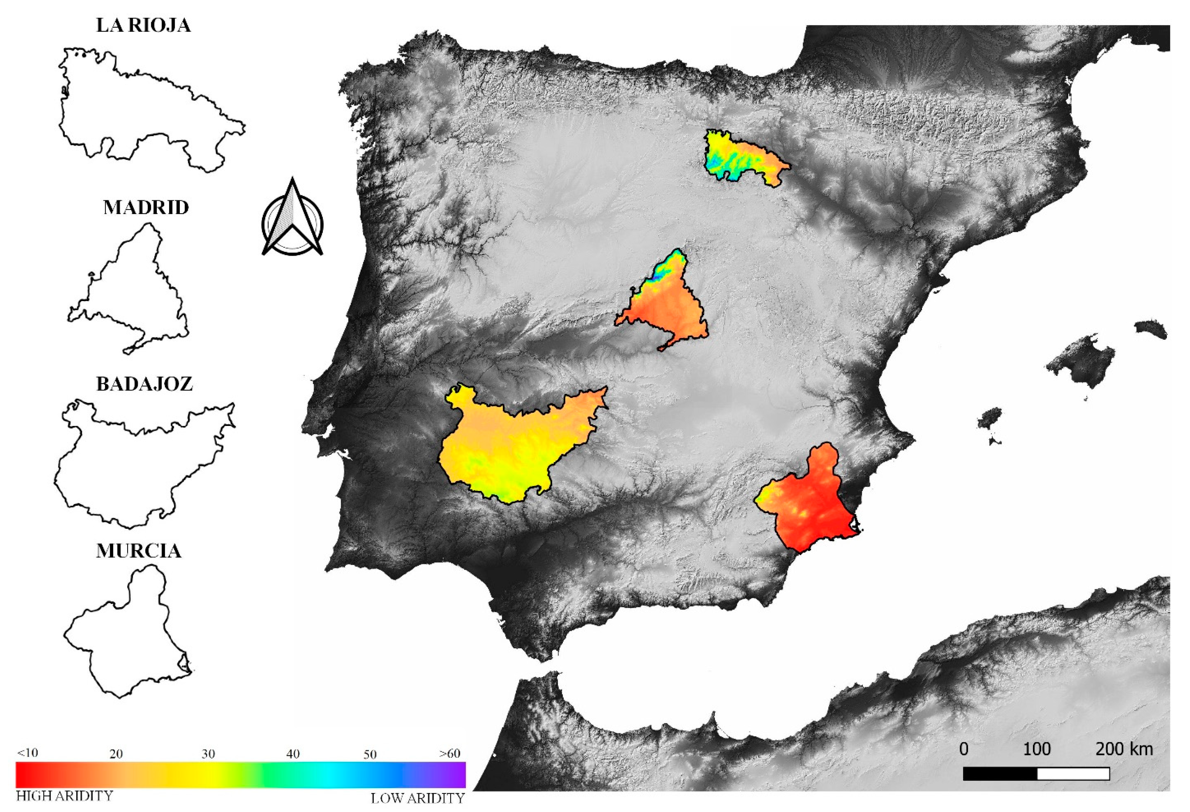
2.1.1. Study Areas

As a result of the topography, ocean influence, and geographical position, the Iberian Peninsula holds a wide range of climatic conditions, with the Mediterranean sub-types being the most common climates [76]. This variability of climates results in a highly functional and structural diversity [77]. We selected four provinces of Spain based on aridity and data availability criteria.
There are several approaches to characterize aridity: based on annual degree-days [78], temperature and precipitation [79], or derived indices using previous variables [80]. We used the Martonne aridity index (M) (Formula (1) [81] due to its simplicity and because it has proven to be useful in areas with marked aridity such as that of our study areas [80,82,83]. We computed M across peninsular Spain as:
M   ( ° C mm ) = P ( T + 10 )  
where T is the mean annual temperature (°C) and P is total annual precipitation (mm) (Table 1). Large values of M are associated with humid conditions. T and P were obtained for each 4th Spanish National Forest Inventory (SNFI-4; 2008 to date) plot from WorldClim2 raster maps with a 1 km resolution [84].
Furthermore, two different criteria were applied to select our study areas: (i) open data from the SNFI-4 and (ii) the second LiDAR coverage (see details in Table 2). Since the SNFI-4 and the LiDAR data are both open access projects, they are planned at the provincial scale (secondary administrative unit in Spain). That is why the selection of the study areas was also done at this scale. The provinces that met our criteria were Badajoz (Southwest), Murcia (Southeast), Madrid (Center), and La Rioja (North), encompassing 2770 field plots.
The study regions covered a wide temperature and precipitation gradient, with La Rioja showing the greatest precipitation and lowest mean annual temperature. In the opposite situation, we found Badajoz and Murcia. These values define a gradient of increasing aridity from north to south and from west to east (see Figure 1, Table 1 for details).

2.1.2. Spanish National Forest Inventory (SNFI)

The field data in this study were obtained from the SNFI-4 for the four provinces in surveys carried out between 2010 and 2017. In Spain, NFI data are taken in 10-year cycles, with the provinces being the sample design unit [85]. The SNFI project establishes plots at 1×1 km UTM grid with a concentric system plot model. The concentric field plots of variable radii measure trees depending on the diameter at breast height (DBH): a radius of 25 m for trees with DBH ≥ 42.5 cm, a radius of 15 m for trees with DBH ≥ 22.5 cm, a radius of 10 m for trees with DBH ≥ 12.5 cm, and a radius of 5 m for trees with a DBH ≥ 7.5 cm. Trees with 2.5 ≤ DBH ≤ 7.5 cm are counted but not measured. For more details about the SNFI data, see Alberdi et al. [28]
We calculated six stand-related variables including basal area (BA; m2 ha−1), density (N; number of stems ha−1), mean plot diameter at breast height (DBH; cm), standard deviation of the DBH (DBHSD; cm), mean height (HM; m), and standard deviation of HM (HMSD; m). These measurements were calculated from tree measurements at plot level by using expansion factors [26] in order to define the different types of forests along the aridity gradient.

2.1.3. Airborne LiDAR Data

LiDAR data used in our study areas were collected between 2016 and 2019 during different surveys carried out for the PNOA-LiDAR project. The point cloud had a point density between 0.5 and 2 points/m2, depending on the province and flight characteristics (see Table 2). LiDAR tiles in LAS format were obtained from the National Geographic Information Centre (http://centrodedescargas.cnig.es/CentroDescargas/buscadorCatalogo.do?coT1amilia=02211#, accessed on 1 November 2021). In total, 17733 tiles were required in order to fully encompass the study areas. A 2-m resolution digital elevation model (DEM) was generated from filtered ground returns and used to normalize the height of the returns. Canopy LiDAR metrics for each SNFI-4 plot were extracted using FUSION/LDV software [86], as well as several scripts developed in MATLAB. Furthermore, we used MATLAB to get metrics that could not get extracted from LiDAR. We applied a predefined height threshold of 2 m to separate trees from understory vegetation with FUSION/LDV, as well as with MATLAB. For each of the field plots, a total of 41 metrics were computed from the normalized point cloud (see Table S3 (Supplementary material)).

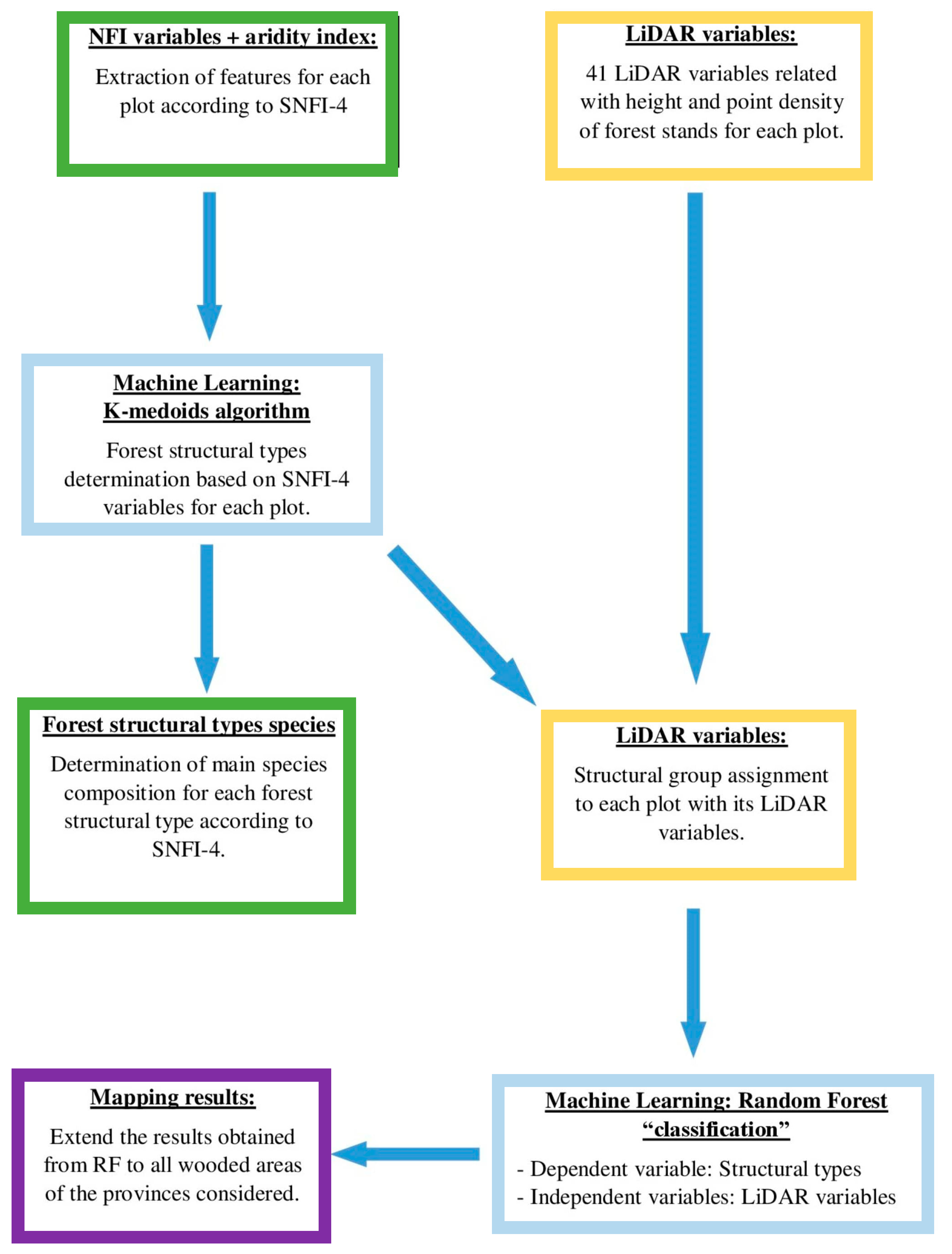
2.2. Determination of Structural Types from SNFI-4 Data

The structural types of the study areas were identified based on six SNFI-4 structural variables (BA, N, HM, HMSD, DBH, and DBHSD) and the aridity index (M) using a k-medoids algorithm. K-medoids is a clustering technique that breaks the dataset into groups, minimizing the distance between points labeled to be in a cluster and a point designated as the center of that cluster [87]. We decided to use a k-medoids algorithm as this approach is more robust than other clustering methods (e.g., k-means) [87]. K-medoids minimizes the sum of dissimilarities of data objects, reducing noise and offering better results when a significant number of outliers are expected. Furthermore, the k-medoids method improves calculations given complex, overlapping data, and it reduces execution time compared with others clustering algorithms [88].
To choose the optimal number of clusters, a gap statistic clustering method was implemented [89]. The gap statistic approach is a standard method for determining the number of clusters in a dataset. The gap statistic method standardizes the graph of log (Wk), where Wk is the within-cluster dispersion, by comparing it to its expectation under an appropriate null reference distribution of the data [90]. The estimate of the optimal clusters corresponds to the value that maximizes the gap statistic (i.e., that yields the largest gap statistic). This means that the clustering structure is far away from the random uniform distribution of points [91]. Interpretation of cluster variables allowed us to define the main structural types found in our study areas. After clustering the SNFI-4 plots, this information served as a reference to classify plots based on LiDAR data.
Once forest structural types were defined, we extracted the species for each structural type from the SNFI-4 in order to determine the main species that made up each forest structural type. Thus, the main species (i.e., those accounting for more than 50% of the total BA of the plots) were assigned to the structural class.

Discrimination of Structural Types from Airborne LiDAR Data

LiDAR data provide detailed descriptions of forest structure; however, the accuracy of LiDAR-based estimates depend on sensor and surveying characteristics [60]. Among them, point density is a critical parameter in determining the accuracy with which structural variables can be obtained from LiDAR [60,61,92]. Moreover, this effect is more important at landscape than at plot scale [93]. Therefore, the ability of low-density airborne LiDAR data to discriminate forest structural types at the province scale was assessed by means of a supervised classification approach using the cluster derived from the SNFI as reference data.
A Random Forest classification (RF) was used to assess the capability of LiDAR metrics to discriminate the forest structures identified from the field data [94]. A summary of the LiDAR metrics is detailed in Table S3 (Supplementary material). The facts that RF (i) allows the detection of nonlinear relations among variables, (ii) considers interactions of different order among predictors, and (iii) can predict categorical variables (as carried out in this case) makes this technique a good option to reach the goal of the study [95].
A first RF model was run to extract the variables with the largest variance importance (calculated through the mean decrease accuracy metric, which evaluated the reduction of model performance when the variable of interest was excluded), obtaining six LiDAR metrics as the most important variables for the model. A second RF model was then run with these variables in order to classify and map forest structural types regionally on LiDAR data. The dataset was randomly split. For both RF, a sample of 70% of the SNFI-4 plots (n = 1938 plots) were used for training the model and the rest 30% of the SNFI-4 plots (n = 832 plots) were using for the validation process. The RF model was set to grow to 500 trees while the parameter of mtry (number of variables randomly sampled as candidates at each split) was one third of the variables. Producer’s accuracy (how often are real features on the ground correctly shown on the classified map or the probability that a certain land cover of an area on the ground is classified as such) and user’s accuracy (how often the class on the map will actually be present on the ground, referred to as reliability) [96] were calculated using the confusion matrix.
The six variables used in the second RF were CCM2, ((All return above 2 m/Total first returns) *100), representing canopy cover; Mean Height of the Canopy Profile (MCHP), represents the relative vertical distribution of canopy surface area (vertical vegetation profile) and accounts for occlusion of the laser energy by the canopy [97]; Area under the canopy curve (AC), related with the forest stand biomass; Percentile 5 (P05) and Percentile 95 (P95) represents height where the 5% and 95%, respectively, are below it; Difference between Percentile 90 and Percentile 50 (Dif 90_50), shows the difference between P90 and P50 and it is related with the biomass location.
Data exploration revealed that the number of plots differs among structural types, i.e., data were unbalanced. This could lead to under-prediction for the less abundant structural types relative to their true proportions because RF attempts to minimize the overall error rate [98]. We solved this issue using a downsampling approach. The downsampling method is a mechanism that reduces the count of training samples falling under the majority class. It helps to even up the counts of target categories [99].
We estimated the overall accuracy of the classification, the omission, and commission errors. While the omission errors refer to those observations that were classified as reference sites that were left out from the correct class in the classification process, the commission errors refer to those observations that were missed in classification in the specific group [100].
All statistical analyses referring to clustering methods were performed using the Nbclust R package [89]. The RF analyses were performed using the randomForest R package [94] in R.4.0.3, R Core Team (2020).

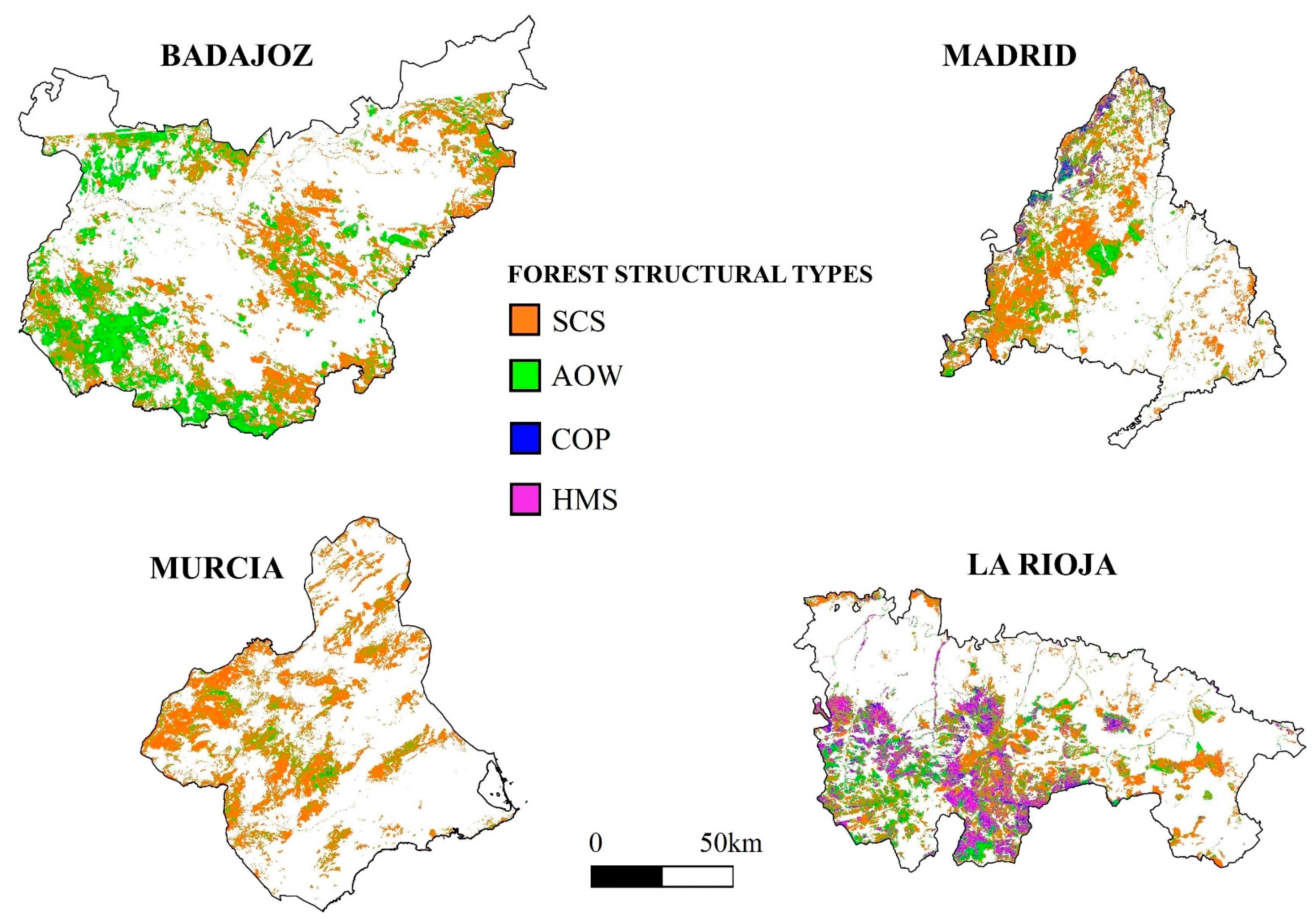
2.3. Regional Forest Structural Types Mapping

Once the RF model for classifying forest structural types was trained and validated, it was applied regionally to identify forest structural type patterns across the four provinces studied and across the aridity gradient. We processed 17,733 tiles and computed the six most important metrics at 50 m resolution, which results in a pixel area close to the area covered by the SNFI plots. We used the Spanish National Forest Map (https://www.miteco.gob.es/es/biodiversidad/servicios/banco-datos-naturaleza/informacion-disponible/T4e50_descargas_ccaa.aspx, accessed on 1 November 2021) to mask forest stands, discarding urban, croplands, or any other land use cover units without woody vegetation cover.
Mapping the forest structural types for each province allowed us to identify spatial patterns of forest structure including boundaries of forest structure along the aridity gradient (Figure 5). See Table S1 for more details (Supplementary material).
To clarify the process of identification, classification, and mapping of forest structural types, Figure 2 shows a flowchart that summarizes the steps followed in our study.

2.4. Downsampling Cloud Point Homogenizing Point Density

In order to assess the point density effect in our model, we downsampled the point cloud density. We took as reference the province with the lowest point density (Murcia, 0.5 p m−2) and reduced the point cloud density of the remaining provinces (La Rioja, 2 p m−2; Madrid, 1 p m−2; and Badajoz, 1 p m−2) to match the point density of Murcia, thus obtaining a homogeneous point density for the four provinces in our study.
Then, we extracted a new set of LiDAR metrics from the downsampled point density data and followed the same process described above to fit the RF model. Finally, we obtained the confusion matrix and evaluated the impact of the point density reduction on the accuracy of the classification.

3. Results

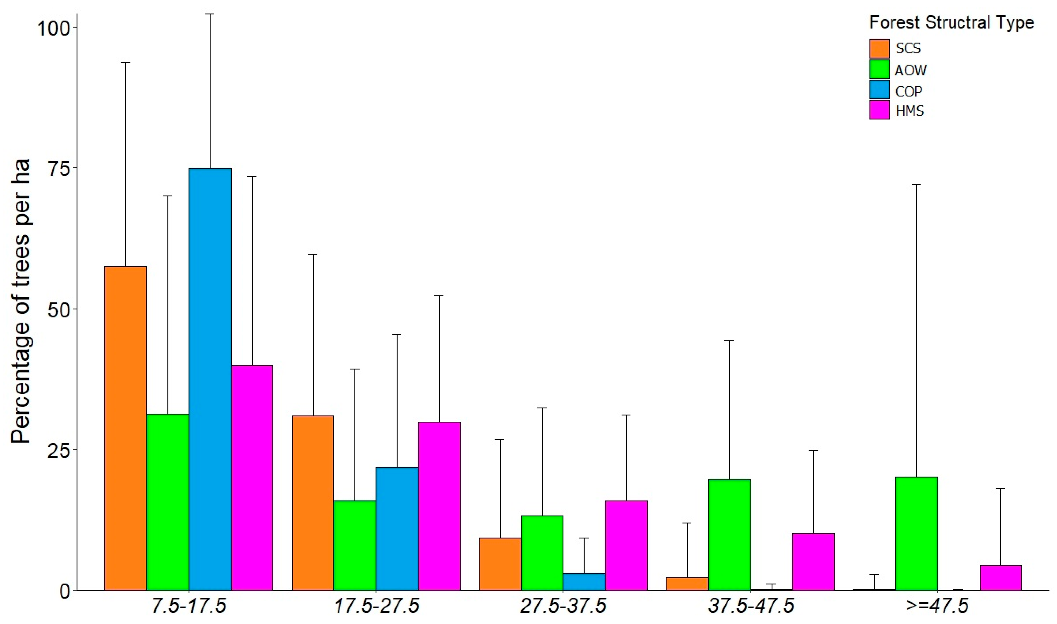
3.1. Forest Structure Based on National Forest Inventories Data

The gap statistic clustering method identified four clusters as the optimal number of forest structural types for the four provinces studied. We assigned names to each cluster based on species composition and aridity values of the structural type. Thus, we will refer hereafter to each typology as (i) Sclerophyllous stands (SCS), (ii) Agrosilvopastoral and/or Open Woodlands (AOW), (iii) Coppices and oromediterranean pines (COP), and (iv) High mountain species (HMS). The structural characteristics of the identified types were summarized in Table 3. SCS was the most common type throughout the gradient, with 40.79% of the total plots located in this type and a wide representation in different provinces. Plots classified as COP represented the lowest percentage with 16.89% of the plots. HMS included 20.97% of our plots, and AOW had 21.37% of the total plots considered in this study (Figure 3).
In relation to the forest inventory variables, COP showed large values of BA and displayed the largest N (Table 3). However, we found that the mean DBH of this structural type was the lowest. As regards the aridity, this structural type, with a value of M = 26, tended to occur in moderately humid sites (i.e., in sites with large values of M). Similarly, HMS also had large values of BA and occurred in humid sites (M = 36.6). However, these stands had a smaller tree density and the mean DBH was larger than in COP. HMS showed the highest value of HM and it displayed a large structural heterogeneity. Regarding AOW, it presented the largest DBH among types, yet was the most variable. This structural type held the lowest density and the second lowest BA. With respect to aridity (M = 21.1), AOW appeared in areas with moderate aridity. SCS showed the lowest value of HM as well as the smallest BA among all structural types. Of the studied sites, this structural type occurred in sites with the highest aridity (M = 18). See Figure 3, Table 3, and Figure S2 (Supplementary material) for more details.
When we evaluated the relative distribution of diameter by classes (Figure 4), an inverse J distribution was suggested for SCS, COP, and HMS, being the lowest diameter class (7.5–17.5 cm) with the largest proportion of trees for the four forest types. This is especially evident for SCS and COP. However, the diameter class with the second largest proportion of trees was 37.5–47.5 cm for AOW. Hence, this forest structural type displayed the largest proportion of big trees (dbh ≥ 37.5 cm) when compared to the other three forest structural types. See Figures S3 and S4 for more details.
Considering all provinces, SCS was the structural type most widely distributed across our study zones, i.e., the structural group that presented the highest abundance of all those evaluated in this work. However, this structural type was consistently more abundant in the south, especially in the province of Murcia. AOW was the second main structural type in our study, and it was also prevalent in the south. In this case, Badajoz had the largest distribution of this structural type. COP and HMS were mostly represented in the provinces with higher M values, Madrid and La Rioja, predominantly in mountain locations where the aridity level was low.

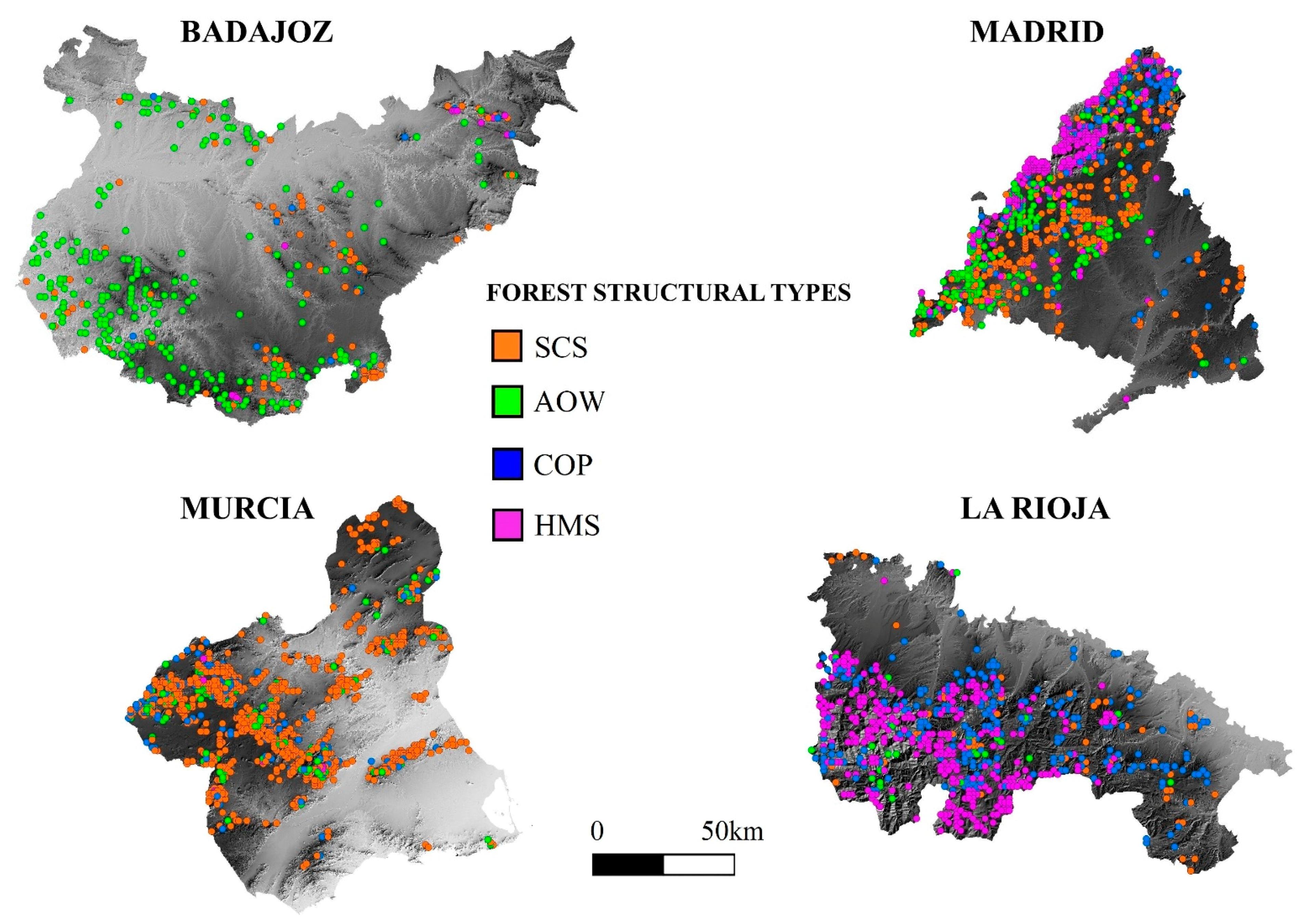
3.2. Discrimination of Forest Structural Types from Airborne LiDAR Data

An initial run of RF, using a downsampling approach, enabled us to identify the most important variables and calibrate a model with balanced data. The six most important variables were, in decreasing order, CC2M ((All return above 2 m/Total first returns) * 100), representing canopy cover; Mean Height of the Canopy Profile (MCHP), related to the biomass through its relation to height; Difference between Percentile 90 and 50 (Dif 90_50), associated with the distribution of biomass within the canopy; Area under the canopy curve (AC), connected to the amount of canopy material; Percentile 5 (P05), linked to the presence of understory; and Percentile 95 (P95), related to canopy height.
The second RF model was run with the six most important variables, obtaining an overall accuracy of 60.63% for the training dataset and 64.18% for the validation dataset, thus showing no overtraining issues. The variance explained by the RF model reached 61.73%. The main classification errors occurred when the RF algorithm classified types AOW and COP as SCS. In fact, the producer’s accuracy for COP and AOW types dropped to values ranging from 36.11% to 41.9% while the accuracy exceeded 69% for HMS and 84% for SCS. The user’s accuracy showed less variability, ranging between 58.59% and 65.55%, with similar values among types (see Table 4 and Table 5).
The performance of the RF with or without the downsampling process (balanced and unbalanced data) was similar in both cases, i.e., quite similar results in analysis with balanced and unbalanced data. However, the prediction of classes increased consistently when we operated with balanced data (Tables S1 and S2 (Supplementary material)). Therefore, the implementation of the downsampling method showed ecologically more coherent results when spatialized (Figure 5). See Figure S1 (Supplementary material) to compare spatialization with and without balanced classes.

3.3. The Effect of Homogenizing Point Cloud Density on Model Accuracy

Once we carried out the downsampling point density analysis, i.e., homogenizing point densities among provinces, we extracted the contingency tables (Supplementary material, Tables S6 and S7). The overall accuracy was 59.3% for the training dataset and 60.7% for the validation dataset.
By forest structural type, we can observe how SCS, AOW, and COP were not affected by downsampling the point density (SCS increase the accuracy 0.5%, AOW reduced the accuracy 4%, and COP increased accuracy 4% for the validation dataset). However, HMS reduced the accuracy by more than 13% with respect to its accuracy before reducing the point density.

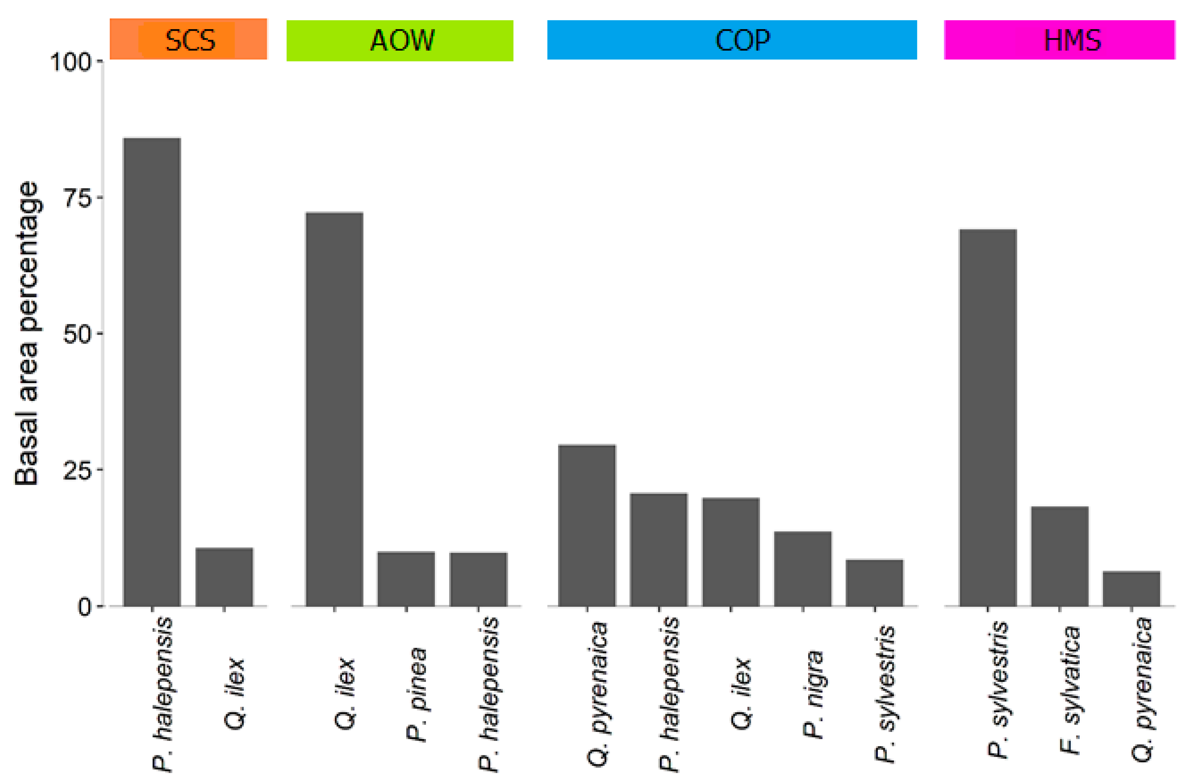
3.4. Species Composition and Forest Structural Types

The results obtained from the extraction of the main species for each structural type using the SNFI-4 show the presence of a wide range of species adapted to different aridity conditions (Figure 6).
SCS was assessed by two main species: P. halepensis, which represented more than 80% of the total BA of the plots contemplated, and Quercus ilex. AOW was composed of up to three main species: Q. ilex, Pinus pinea L., and P. halepensis. However, Q. ilex represented more than 60% of the total BA of the plots. COP was composed of several ecologically distinct species. In decreasing basal area abundance: Quercus pyrenaica Willd., Pinus halepensis Mill, Quercus ilex L, Pinus nigra Arn., and Pinus sylvestris L. Three main species comprised HMS: P. sylvestris, Fagus sylvatica L., and Q. pyrenaica. In this structural type, P. sylvestris represented more than 60% of the total BA. F. sylvatica and Q. pyrenaica made up, in decreasing order of abundance, the rest of the BA of the plots.

4. Discussion

4.1. Low-Density LiDAR Data Considerations

In this study, we have identified and described variations in forest structure along the Mediterranean-temperate forest ecotone by combining low point density LiDAR, NFI, and climate data.
Once we extracted the forest stand variables and M was calculated for each plot, a k-medoids algorithm was implemented obtaining four structural types for the aridity gradient contemplated in our study. Many studies have implemented different clustering methods to define and classify forest structure [17,55,56]. For example, Abdullahi et al. [101] applied a k-means approach to classify forest structure based on height information derived from interferometric X-band Synthetic Aperture Radar. Moran et al. [102] utilized a hierarchical clustering algorithm to estimate forest structure classes using high point density airborne LiDAR data in Montana, USA. As seen, there are different ways to group forest structures. However, Wallace et al. [103] advised that hierarchical solutions were not as effective as nonhierarchical approaches, at least in stands where the forest structure is not homogeneous. We advocated non-hierarchical clustering methods for three main reasons: (i) it is difficult to update hierarchies without rebuilding the classification from scratch, (ii) acknowledging reticular relationships between vegetation types is more realistic than imposing a hierarchical structure [103], and (iii) concentrating on the definition of types does not preclude imposing a further structure a posteriori [104]. Following these conclusions, and because of the complexity of the Mediterranean forest structure, we chose a nonhierarchical method to cluster our structural types.
There are multiple examples where forest structure was defined directly using LiDAR data information [57,105,106,107,108]. However, in those studies, high point density LiDAR data were used, providing high levels of accuracy. Since the PNOA LiDAR project contains low point density, we decided to define forest structural types through SNFI-4 firstly, instead of attempting to discriminate forest structural groups directly from the LiDAR data. In this way, the structural characteristics of each group are defined from field data that are subsequently used to train a supervised algorithm that discriminates such groups from LiDAR variables, describing different aspects of forest structure.
With respect to the LiDAR variables selected, we found CC2M, MCHP, Dif 90_50, AC, P05, and P95 (see Table S1 (Supplementary material)) the most important variables to discriminate forest structural types. Görgens et al. [109] pointed out that metrics selected using automated processes might differ completely between studies and thus require the identification of stable metrics to be used as predictors to facilitate model generalization (see also [110,111]). For instance, Valbuena et al. [55] used a methodology for automated classification of forest areas from LiDAR datasets based on two direct metrics: L-coefficient of variation and L-skewness. Torresan et al. [17] utilized standard deviation and canopy mode heights, percentile 95, percentile 99, and the difference between percentile 90 and percentile 10. Despite each study selecting different metrics, many of the LiDAR-derived metrics are strongly correlated [112]. Moreover, the metrics selected in all studies represent complementary aspects of the 3D structure of forest stands. Huesca et al. [113] defined forest structural types based on metrics describing the horizontal structure and another set of metrics describing the vertical structure of forests. In our study, the selected metrics described both aspects of forest structure: CC2M described the canopy cover; P95 and MCHP were related to the mean and dominant height of the canopy [114]; AC and Dif 90_50 were associated with biomass and its distribution through the canopy [92,115], respectively; and P05 was related to the presence of understory strata. These metrics provide a comprehensive description of the vertical and horizontal distribution of the forest.
The overall accuracy in our study was 60.63% and 64.18% for the training and the validation set, respectively. These results outperformed other studies carried out in Mediterranean environments, despite the low point density of our datasets. For instance, Torresan et al. [17], using an agglomerative hierarchical clustering and point density of 1.28 p m−2, detected five clusters of forest structure in the province of Trento (Italy) using DBH. They attained an overall accuracy of 54.1%, lower than the overall accuracy obtained in our study. Valbuena et al. [55] obtained an overall accuracy above 80% using L-coefficient of variation and L-skewness ALS metrics to classify boreal forest types with a point density of approx. 1 p m−2. They conducted their study in Finland, where forest areas are much more structurally homogeneous than those in Mediterranean environments [116]. However, it was also remarkable that Valbuena et al. [55] considered only two LiDAR metrics, defining forest as open and closed canopies and even-size and uneven-sized trees (two by two), depending on the metric value. In our study, we took into account a total of four structural types defined using six LiDAR variables, which could reduce the accuracy of our classification because of the complexity of the structural groups.
It should be noted that it was not only the structural complexity of the studied places, but also the total spatial extent of such. For example, Adnan et al. [56] developed a methodology to classify forest structural types across bioregions applying a hierarchical clustering analysis to determine forest structural types in coniferous and deciduous forests using NFI variables. They achieved an overall accuracy between 72% and 87%, depending on the functional type (deciduous vs. coniferous). It was also noteworthy that Adnan et al. [56] considered a total of 566 plots, while in our study we contemplated 2770 plots. The large spatial extent we considered in our study allowed us to detect variations along the aridity gradient in relation to the forest structure. However, this large spatial extent could be considered a drawback, since, when considering a large area, we obtain high spatial variability which could influence the accuracy of our model to detect the structural types defined in the study [93].
The producer’s accuracy achieved in our study ranged between 36.11% and 84.93% for the validation dataset, whereas user’s accuracy remained more consistent for all classes. The highest producer’s accuracy was reached for the classification of SCS (84.93%). This could be because SCS is the most frequent class in the study regions as well as the most homogeneous group in terms of forest structure. The low accuracy obtained for some of our structural types could be due to their structural complexity. When the structural complexity of forests increases, the accuracy of laser metrics can be affected due to the interference of middle forest strata [117], particularly when using low density data. This fact coincides with other studies like Torresan et al. [17] where the presence of middle strata, or even understory, caused considerable impact to the density of LiDAR points below the canopy, thus affecting the accuracy of the analyses [118].
The literature shows a general tendency to decrease the producer’s accuracy with stand density, relative tree height, presence of forest understory, or tree clustering [119,120]. In line with this tendency, our producer’s accuracy decreased in structural groups with high density and moderate stand height (COP). The producer’s accuracy also tended to decrease when we classified structural groups where trees are usually clustered and there are abundant middle and understory strata (AOW). Moreover, low density data have only a moderate ability to predict stand density [17,120,121]. On the other hand, in groups with moderate tree density, where stands tend to be more homogeneous, our producer’s accuracy increased consistently (SCS-HMS).
The user’s accuracy achieved moderately satisfactory results in terms of classification performance. Considering that the user’s accuracy shows the suitability of the choice and identification of forest groups [41], we can argue that our user’s accuracy is highly homogeneous among forest structure types (between 58.59% and 65.55%). Furthermore, given the spatial extension considered in our study, the high number of observations along the aridity gradient, and the heterogeneity of Mediterranean forests, our results can be considered satisfactory.
When we considered the downsampling point cloud density results, we observed that the accuracy of SCS, AOW, and COP remained the same as before the downsampling process (less than 4% difference). These forest structural types were mainly located in provinces where the point density was lower before the downsampling point density analysis (see Figure 3 and Figure 5), i.e., provinces with similar original point cloud density. However, HMS reduced the accuracy by 13% with and without downsampling point density, respectively. HMS is mainly located in La Rioja, the province with the highest point density before the downsampling process. This result is coincident with those results from Disney et al., Leitold et al., García et al. [59,60,61], which show how point density had a significant impact on the accuracy of structural forest variables. It is also remarkable, as mentioned before [17,120,121], that low point density LiDAR presents a moderate capacity to predict forest stand density.
It should be noted that increasing the point cloud density could improve the results obtained in this and similar studies where forest structure is being defined. As it is observed in this study, HMS worsened its accuracy when we downsampled point density; demonstrating that when a denser point cloud is contemplated, results can significantly improve. To that end, and due to the capacity of the new sensors developed during the last few years, it is possible to increment the point cloud density at the national level in the 3rd PNOA-LiDAR coverage until around 5 p m−2 (M. Jurado, personal communication).
Another important factor affecting the achieved accuracy when we evaluated forest stand variables and structure was the time lapse between the NFI data and LiDAR data collection [122]. In our study, the time lapse between SNFI-4 and LiDAR data collection ranged from 1–2 years in Badajoz to 6–7 years in Murcia. The time difference in Madrid was 3–4 years, and 4 years in La Rioja. These differences between data collections likely affected the accuracy of our study, especially when we were evaluating possible transitional forest structural types, such as that considered in COP.

4.2. Species Composition and Forest Structural Types

The results obtained from the extraction of the main species for each structural type showed the utility of using NFI to figure out the species conforming to our structural types (Figure 6). In fact, without NFI, it would not be possible to identify these species only with LiDAR.
COP was composed of stands of oromediterranean species such as P. nigra, P. sylvestris and, mainly, of low forest resprouting species such as Q. pyrenaica and Q. ilex [123,124]. This type is related to highly densified structures, both resulting from older pine afforestation and abandoned coppiced stand, but also post-disturbance (i.e., fire), high density stands. The low diameters characterizing low forests may explain the high proportion of small trees in the histogram of frequencies of trees by diameter class (Figure S4, supplementary material) as well as the low mean DBH. In addition, this structural type was present in riparian forests, especially in central and northern Iberian Peninsula, where aridity is generally lower. Species like Populus spp., Fraxinus angustifolia Vahl., or other species with a tall stature were part of these forests [125]. HMS shared a similar ecological space with COP, although it occurred in sites that were more humid. These stands presented larger DBH and lower N than COP. This forest type aggregated mature individuals of montane species such as P. sylvestris, F. sylvatica, Q. pyrenaica [126]. The diametric distribution for this type also followed an inverse J but it was more flattened than in the case of SCS and COP. To some extent, these two facts could be due to: (i) these species occupy many areas with low accessibility where the wood extraction is limited, and (ii) forest management prescription usually promotes large diameters to obtain high-value by-products. This forest structural type was also present by riversides, sharing species with COP. AOW corresponded to agrosilvopastoral systems related to more or less open woodlands and savanna-like formations (namely dehesas or montados) and it was composed mainly of Q. ilex [127,128]. In agreement with our results, these stands usually display low tree density and high plot diameter. Low rates of regeneration and small trees are also characteristic of these forests, threatening the persistence of these stands. Finally, SCS forests were made up of drought-adapted species such as Q. ilex and P. halepensis [129,130,131]. The warm and dry climatic conditions and the asexual reproduction of Q. ilex could be behind the low mean diameter found for this forest type. These results overall provided a compositional description of our forest structural types.
The distribution of the structural types was partially segregated along climatic gradients. SCS was more abundant towards south and east, Murcia being the most arid province under study and presenting the highest relative extent of this structural type. This structure was coincident in space and plot mensuration data for forest structures described in previous studies for the southeast of Spain [132,133]. In our study zones, AOW had its largest and most continuous occurrence in the province of Badajoz. This result could be due to the presence of open woodlands, which are characterized by low densities, and in our study areas, they were mainly found in Badajoz [134]. HMS was essentially distributed through the high part of the mountains, mainly located in the north of Madrid, and the south and central areas of La Rioja. HMS was also observed along rivers. The species composition and distribution were similar to that described by López Estéban [135] for the Spanish central mountains and by Arnáez et al. [136] for the region of La Rioja. Finally, COP occupied similar ecological locations to those of HMS, but in places with higher aridity. This structural type showed the smallest occurrence among the structural types considered for this study. This condition could be due to its particular position in the aridity gradient [137].
These four structural typologies suggest divergent functional performance in terms of exposure and vulnerability (sensitivity and adaptive capacity) in response to climate change hazards (chiefly hot spells and intense droughts, windstorms, and wildfires). Therefore, their description can be assisted to the definition of adaptation priority regions (i.e., targeting thinning in order to decrease drought vulnerability) (COP) or alternative plantations to foster recruitment (AOW).

4.3. Other Methodological Remarks

Forest structure refers to the three-dimensional arrangement of vegetation (especially focused on trees) considered at a range of spatial scales, in combination with nonliving spatial elements such as soils, slopes, and hydrology [138]. Due to the interpretability of the term “forest structure” and its definition, there is a wide range of studies where different variables have been used to discriminate forest structural types. Torresan et al. [17] utilized DBH to classify forest structure stands into understory, midstory, and overstory. However, we considered that for regional studies like ours, taking only one structural variable would make us spatially underestimate the real structure of the forest stands present in peninsular Spain. Adnan et al. [56] used four forest structural variables to classify forest structure: quadratic mean diameter (QMD), Gini coefficient (GC), basal area larger than mean (BALM), and density of stems (N). In our study, we included BA, DBH, and DBHSD, which integrate QMD and BALM. GC is an index of inequality utilized in ecology to determine tree size variability [55]. Instead, we utilized HM and HMSD as an indicator of stand height variability. These two variables, plus DBH and DBHSD, accounted for the variability attributable to the different allometries (i.e., DBH–HM relationship), along with growth among species, site conditions, and stand development stage. The chosen variables N and BA allowed us to differentiate fully stocked forest types from medium or open stands [129,131,139,140]. Similar to our approach, De Cáceres et al. [141] developed a general method to classify forest stands using species composition and the forest structure variables BA, DBH, and HM.
Regarding data accuracy, airborne LiDAR scanners are highly accurate nowadays [38], so the LiDAR-based estimates are related to factors like point density, modeling process (ALS metrics, modeling approach, training data size), plot co-registration, forest composition, etc. [142,143,144]. In this direction, we had into account for those requirements in order to ensure a correct design and treatment of LiDAR data.
Improving the knowledge about forest structure in large areas remains a priority in forest ecology [18,19], especially in ecosystems highly exposed to climate change [145,146]. However, many studies carried out using LiDAR data to predict forest structure were completed using a relatively small spatial extent [18,147,148]. Conversely, our study contemplated four ecologically distinct Spanish provinces that comprise 10.6% of the total forest area of Spain [149]. The geographical location of the provinces and the large number of plots considered therein provided a well-defined aridity gradient so that our sample is representative of the main structural types present in peninsular Spain.
The analysis and methodology developed in this study can guide decision-making regarding Mediterranean forest management, resource use, and ecosystem services. The maps developed in this work can also be used to communicate different forest biodiversity conservation issues, e.g., landscape fragmentation of different forest types [150]. The identification and distribution of these forest structures on a regional, or even national scale, allow us to prioritize specific actions for forest ecosystem management and conservation.

5. Conclusions

We evaluated the usefulness of low-density discrete return airborne LiDAR data to predict forest structural types identified with National Forest Inventories along a wide aridity gradient covering peninsular Spain. The identification of Spanish forest structural types considering climatological variables opens an interesting window to support and strengthen current forest management, conservation, and monitoring programs. Despite our model having achieved a satisfactory overall accuracy, there is a considerable margin for improvement through the densification of the LiDAR data point cloud, as well as concurrent data field collection. The classification of forest structural types proposed is interesting for the management and protection of Mediterranean forests, prevention of natural disasters, and conservation of ecosystem services. Furthermore, our methodology can be adapted to detect and analyze changes over space and time, especially considering that the PNOA includes multitemporal LiDAR coverage for the whole of the Spanish territory. These previous considerations will allow us to develop better monitoring of forest stands and their progression, giving us a vision on a national scale of the different Spanish forests and their evolution.

Supplementary Materials

The following are available online at https://0-www-mdpi-com.brum.beds.ac.uk/article/10.3390/rs14010235/s1, Table S1: Number of pixels and percentages (in brackets) of each structural type by province with balanced classes. SCS: Sclerophyllous stands; AOW: Agrosilvopastoral and/or Open Woodlands; COP: Coppices and oromediterranean pines; HMS: High mountain species. Table S2: Number of pixels and percentages (in brackets) of each structural type by province with no balanced classes. SCS: Sclerophyllous stands; AOW: Agrosilvopastoral and/or Open Woodlands; COP: Coppices and oromediterranean pines; HMS: High mountain species. Table S3: LiDAR metrics and abbreviations. Table S4: Kruskal-Wallis rank sum test. Table S5: Pairwise comparisons using Wilcoxon rank sum test with continuity correction. P-value adjustment method: holm. SCS: Sclerophyllous stands; AOW: Agrosilvopastoral and/or Open Woodlands; COP: Coppices and oromediterranean pines; HMS: High mountain species. Table S6: Contingency table for the training dataset. T3: Forest structural type 1; T2: Forest structural type 2; T3: Forest structural type 3; T4: Forest structural type 4. Table S7: Contingency table for the training dataset. SCS: Sclerophyllous stands; AOW: Agrosilvopastoral and/or Open Woodlands; COP: Coppices and oromediterranean pines; HMS: High mountain species. Table S8: LiDAR flight and sensor characteristics. Figure S1: Distribution of forest structural type per province with no balanced classes. SCS: Sclerophyllous stands; AOW: Agrosilvopastoral and/or Open Woodlands; COP: Coppices and oromediterranean pines; HMS: High mountain species. Figure S2: Martonne aridity index per forest structural type. SCS: Sclerophyllous stands; AOW: Agrosilvopastoral and/or Open Woodlands; COP: Coppices and oromediterranean pines; HMS: High mountain species. Figure S3: Plot basal area per hectare per cluster. SCS: Sclerophyllous stands; AOW: Agrosilvopastoral and/or Open Woodlands; COP: Coppices and oromediterranean pines; HMS: High mountain species. Figure S4: Number of trees per per hectare per cluster. SCS: Sclerophyllous stands; AOW: Agrosilvopastoral and/or Open Woodlands; COP: Coppices and oromediterranean pines; HMS: High mountain species.

Author Contributions

J.T.-T.: Statistical analysis, Writing—original draft preparation. D.M.-F.: Writing—Reviewing & Editing. M.A.Z.: Writing—Reviewing & Editing, Funding Acquisition. J.A.: data gathering, Resources, Editing. M.G.: Writing—Reviewing & Editing, Funding Acquisition, Conceptualization, Methodology. All authors have read and agreed to the published version of the manuscript.

Funding

This work was supported by grant DARE (RTI2018-096884-B-C32; MICINN, Spain). J.T.-T. was supported by the Community of Madrid Region under the framework of the multi-year agreement with the University of Alcalá (Stimulus to Excellence for Permanent University Professors, EPU-INV/2020/010). The Spanish Ministry of Science supported DMF through the Juan de la Cierva Formación program (FJC2018-037870-I). J.A. was supported by a FPI fellowship of the Department of Education of the Basque Government.

Data Availability Statement

The datasets and R code used for the development of this work are available upon request to the author Data analyzed in this study were extracted from the following web addresses: LiDAR data: http://centrodedescargas.cnig.es/CentroDescargas/catalogo.do?Serie=LIDAR (accessed on 1 November 2021). National Forest Inventory data*: https://www.miteco.gob.es/es/biodiversidad/servicios/banco-datos-naturaleza/informacion-disponible/ifn3.aspx (accessed on 1 November 2021). *data from the fourth National Forest Inventory are not currently available to the public as of publication of this paper.

Acknowledgments

We thank the Ministry of Agriculture, Fisheries and Food (MAPA) for access to the Spanish Forest Inventory. We also acknowledge the research program ‘Estímulo a la Excelencia para Profesores Universitarios Permanentes’ funded by the University of Alcalá and the Community of Madrid (EPU-INV/2020/009) and the set of grants for carrying out projects to promote the Creation and Consolidation of Research Groups (CG20/CC-005). The authors thank Elizabeth Hayden Sloan for revising the English grammar and Paloma Ruiz-Benito for helping with SNFI data and critical comments to previous versions of the manuscript.

Conflicts of Interest

The authors have no conflict of interest to declare. All co-authors have seen and agree with the contents of the manuscript. We certify that the submission is original work and is not under review at any other publication.

References

  1. Bohn, F.J.; Huth, A. The importance of forest structure to biodiversity-productivity relationships. R. Soc. Open Sci. 2017, 4, 160521. [Google Scholar] [CrossRef] [Green Version]
  2. Lelli, C.; Bruun, H.H.; Chiarucci, A.; Donati, D.; Frascaroli, F.; Fritz, Ö.; Goldberg, I.; Nascimbene, J.; Tøttrup, A.P.; Rahbek, C.; et al. Biodiversity response to forest structure and management: Comparing species richness, conservation relevant species and functional diversity as metrics in forest conservation. For. Ecol. Manag. 2019, 432, 707–717. [Google Scholar] [CrossRef]
  3. Pereira, P.; Úbeda, X.; Martin, D.; Mataix-Solera, J.; Cerdà, A.; Burguet, M. Wildfire effects on extractable elements in ash from a Pinus pinaster forest in Portugal. Hydrol. Process. 2014, 28, 3681–3690. [Google Scholar] [CrossRef]
  4. Gonsalves, L.; Law, B.; Blakey, R. Experimental evaluation of the initial effects of large-scale thinning on structure and biodiversity of river red gum (Eucalyptus camaldulensis) forests. Wildl. Res. 2018, 45, 397–410. [Google Scholar] [CrossRef]
  5. Pretzsch, H.; Bielak, K.; Block, J.; Bruchwald, A.; Dieler, J.; Ehrhart, H.-P.; Kohnle, U.; Nagel, J.; Spellmann, H.; Zasada, M.; et al. Productivity of mixed versus pure stands of oak (Quercus petraea (M att.) L iebl. and Quercus robur L.) and European beech (Fagus sylvatica L.) along an ecological gradient. Eur. J. For. Res. 2013, 132, 263–280. [Google Scholar] [CrossRef]
  6. Williams, A.P.; Allen, C.D.; Millar, C.I.; Swetnam, T.W.; Michaelsen, J.; Still, C.J.; Leavitt, S.W. Forest responses to increasing aridity and warmth in the southwestern United States. Proc. Natl. Acad. Sci. USA 2010, 107, 21289–21294. [Google Scholar] [CrossRef] [PubMed] [Green Version]
  7. Gómez-Aparicio, L.; García-Valdés, R.; Ruiz-Benito, P.; Zavala, M.A. Disentangling the relative importance of climate, size and competition on tree growth in Iberian forests: Implications for forest management under global change. Glob. Chang. Biol. 2011, 17, 2400–2414. [Google Scholar] [CrossRef] [Green Version]
  8. Ruiz-Benito, P.; Lines, E.R.; Gómez-Aparicio, L.; Zavala, M.A.; Coomes, D.A. Patterns and Drivers of Tree Mortality in Iberian Forests: Climatic Effects Are Modified by Competition. PLoS ONE 2013, 8, e56843. [Google Scholar] [CrossRef] [Green Version]
  9. Condés, S.; del Rio, M. Climate modifies tree interactions in terms of basal area growth and mortality in monospecific and mixed Fagus sylvatica and Pinus sylvestris forests. Eur. J. For. Res. 2015, 134, 1095–1108. [Google Scholar] [CrossRef]
  10. Park, J.; Kim, T.; Moon, M.; Cho, S.; Ryu, D.; Kim, H.S. Effects of thinning intensities on tree water use, growth, and resultant water use efficiency of 50-year-old Pinus koraiensis forest over four years. For. Ecol. Manag. 2018, 408, 121–128. [Google Scholar] [CrossRef]
  11. Seidl, R.; Schelhaas, M.-J.; Lexer, M.J. Unraveling the drivers of intensifying forest disturbance regimes in Europe. Glob. Chang. Biol. 2011, 17, 2842–2852. [Google Scholar] [CrossRef]
  12. Marqués, L.; Zavala, M.A.; Camarero, J.J.; Hartig, F.; Madrigal-González, J. Last-century forest productivity in a managed dry-edge Scots pine population: The two sides of climate warming. Ecol. Appl. 2018, 28, 95–105. [Google Scholar] [CrossRef]
  13. Madrigal-González, J.; Ballesteros-Cánovas, J.A.; Zavala, M.A.; Morales-Molino, C.; Stoffel, M. Forest stocks control long-term climatic mortality risks in Scots pine dry-edge forests. Ecosphere 2020, 11. [Google Scholar] [CrossRef]
  14. Astigarraga, J.; Andivia, E.; Zavala, M.A.; Gazol, A.; Cruz-Alonso, V.; Vicente-Serrano, S.M.; Ruiz-Benito, P. Evidence of non-stationary relationships between climate and forest responses: Increased sensitivity to climate change in Iberian forests. Glob. Chang. Biol. 2020, 26, 5063–5076. [Google Scholar] [CrossRef] [PubMed]
  15. McDowell, N.G.; Allen, C.D.; Anderson-Teixeira, K.; Aukema, B.H.; Bond-Lamberty, B.; Chini, L.; Clark, J.S.; Dietze, M.; Grossiord, C.; Hanbury-Brown, A.; et al. Pervasive shifts in forest dynamics in a changing world. Science 2020, 368. [Google Scholar] [CrossRef] [PubMed]
  16. Plas, F.; Ratcliffe, S.; Ruiz-Benito, P.; Scherer-Lorenzen, M.; Verheyen, K.; Wirth, C.; Zavala, M.A.; Ampoorter, E.; Baeten, L.; Barbaro, L.; et al. Continental mapping of forest ecosystem functions reveals a high but unrealised potential for forest multifunctionality. Ecol. Lett. 2018, 21, 31–42. [Google Scholar] [CrossRef] [PubMed] [Green Version]
  17. Torresan, C.; Corona, P.; Scrinzi, G.; Marsal, J.V. Using classification trees to predict forest structure types from LiDAR data. Ann. For. Res. 2016, 59. [Google Scholar] [CrossRef]
  18. Neuville, R.; Bates, J.; Jonard, F. Estimating Forest Structure from UAV-Mounted LiDAR Point Cloud Using Machine Learning. Remote Sens. 2021, 13, 352. [Google Scholar] [CrossRef]
  19. Moreno-Fernández, D.; Cañellas, I.; Alberdi, I.; Montes, F. Improved stand structure characterization from nested plot designs in the Spanish National Forest Inventory. For. An Int. J. For. Res. 2021, 94, 244–257. [Google Scholar] [CrossRef]
  20. Scholes, R.J.; Dowty, P.R.; Caylor, K.; Parsons, D.A.B.; Frost, P.G.H.; Shugart, H.H. Trends in savanna structure and composition along an aridity gradient in the Kalahari. J. Veg. Sci. 2002, 13, 419–428. [Google Scholar] [CrossRef]
  21. Dodson, E.K.; Ares, A.; Puettmann, K.J. Early responses to thinning treatments designed to accelerate late successional forest structure in young coniferous stands of western Oregon, USA. Can. J. For. Res. 2012, 42, 345–355. [Google Scholar] [CrossRef]
  22. Restaino, C.; Young, D.J.N.; Estes, B.; Gross, S.; Wuenschel, A.; Meyer, M.; Safford, H. Forest structure and climate mediate drought-induced tree mortality in forests of the Sierra Nevada, USA. Ecol. Appl. 2019, 29, e01902. [Google Scholar] [CrossRef] [PubMed]
  23. Khabarov, N.; Krasovskiy, A.; Obersteiner, M.; Swart, R.; Dosio, A.; San-Miguel-Ayanz, J.; Durrant, T.; Camia, A.; Migliavacca, M. Forest fires and adaptation options in Europe. Reg. Environ. Chang. 2016, 16, 21–30. [Google Scholar] [CrossRef] [Green Version]
  24. Bussotti, F.; Pollastrini, M.; Holland, V.; Brüggemann, W. Functional traits and adaptive capacity of European forests to climate change. Environ. Exp. Bot. 2015, 111, 91–113. [Google Scholar] [CrossRef]
  25. Lindner, M.; Maroschek, M.; Netherer, S.; Kremer, A.; Barbati, A.; Garcia-Gonzalo, J.; Seidl, R.; Delzon, S.; Corona, P.; Kolström, M.; et al. Climate change impacts, adaptive capacity, and vulnerability of European forest ecosystems. For. Ecol. Manag. 2010, 259, 698–709. [Google Scholar] [CrossRef]
  26. Chirici, G.; Winter, S.; McRoberts, R.E. National Forest Inventories: Contributions to Forest Biodiversity Assessments; Springer Science & Business Media: Cham, Switzerland, 2011; Volume 20. [Google Scholar]
  27. Ruiz-Benito, P.; Vacchiano, G.; Lines, E.R.; Reyer, C.P.; Ratcliffe, S.; Morin, X.; Hartig, F.; Mäkelä, A.; Yousefpour, R.; Chaves, J.E.; et al. Available and missing data to model impact of climate change on European forests. Ecol. Model. 2020, 416, 108870. [Google Scholar] [CrossRef]
  28. Álvarez-González, J.G.; Canellas, I.; Alberdi, I.; Gadow, K.; González, A.D.R. National Forest Inventory and forest observational studies in Spain: Applications to forest modeling. For. Ecol. Manag. 2014, 316, 54–64. [Google Scholar] [CrossRef]
  29. Reque, J.A.; Bravo, F. Identifying forest structure types using National Forest Inventory Data: The case of sessile oak forest in the Cantabrian range. Investig. Agrar. Sist. Recur. 2008, 17, 105. [Google Scholar] [CrossRef] [Green Version]
  30. Garcia, M.; Saatchi, S.; Ustin, S.; Balzter, H. Modelling forest canopy height by integrating airborne LiDAR samples with satellite Radar and multispectral imagery. Int. J. Appl. Earth Obs. Geoinf. 2018, 66, 159–173. [Google Scholar] [CrossRef]
  31. Durán, J.V. Los inventarios forestales nacionales: Una herramienta para la gestión, la planificación y la investigación. Foresta 2013, 57, 34–41. [Google Scholar]
  32. Simard, M.; Pinto, N.; Fisher, J.; Baccini, A. Mapping forest canopy height globally with spaceborne lidar. J. Geophys. Res. Biogeosci. 2011, 116. [Google Scholar] [CrossRef] [Green Version]
  33. Guo, X.; Coops, N.C.; Tompalski, P.; Nielsen, S.E.; Bater, C.W.; Stadt, J.J. Regional mapping of vegetation structure for biodiversity monitoring using airborne lidar data. Ecol. Inform. 2017, 38, 50–61. [Google Scholar] [CrossRef]
  34. Deo, R.K.; Russell, M.B.; Domke, G.M.; Woodall, C.W.; Falkowski, M.J.; Cohen, W.B. Using Landsat Time-Series and LiDAR to Inform Aboveground Forest Biomass Baselines in Northern Minnesota, USA. Can. J. Remote Sens. 2017, 43, 28–47. [Google Scholar] [CrossRef]
  35. Beaudoin, A.; Bernier, P.Y.; Guindon, L.; Villemaire, P.; Guo, X.J.; Stinson, G.; Bergeron, T.; Magnussen, S.; Hall, R.J. Mapping attributes of Canada’s forests at moderate resolution through kNN and MODIS imagery. Can. J. For. Res. 2014, 44, 521–532. [Google Scholar] [CrossRef] [Green Version]
  36. Ruiz, L.; Recio, J.A.; Crespo-Peremarch, P.; Sapena, M. An object-based approach for mapping forest structural types based on low-density LiDAR and multispectral imagery. Geocarto Int. 2018, 33, 443–457. [Google Scholar] [CrossRef]
  37. Wulder, M.; White, J.; Alvarez, F.; Han, T.; Rogan, J.; Hawkes, B. Characterizing boreal forest wildfire with multi-temporal Landsat and LIDAR data. Remote Sens. Environ. 2009, 113, 1540–1555. [Google Scholar] [CrossRef]
  38. McRoberts, R.E.; Tomppo, E.O. Remote sensing support for national forest inventories. Remote Sens. Environ. 2007, 110, 412–419. [Google Scholar] [CrossRef]
  39. McRoberts, R.E.; Chen, Q.; Gormanson, D.D.; Walters, B. The shelf-life of airborne laser scanning data for enhancing forest inventory inferences. Remote Sens. Environ. 2018, 206, 254–259. [Google Scholar] [CrossRef]
  40. Pascual, A.; Guerra-Hernández, J.; Cosenza, D.N.; Sandoval-Altelarrea, V. Using enhanced data co-registration to update Spanish National Forest Inventories (NFI) and to reduce training data under LiDAR-assisted inference. Int. J. Remote Sens. 2021, 42, 126–147. [Google Scholar] [CrossRef]
  41. Wiggins, H.L.; Nelson, C.R.; Larson, A.J.; Safford, H.D. Using LiDAR to develop high-resolution reference models of forest structure and spatial pattern. For. Ecol. Manag. 2019, 434, 318–330. [Google Scholar] [CrossRef]
  42. Kane, V.R.; Bakker, J.D.; McGaughey, R.J.; Lutz, J.; Gersonde, R.F.; Franklin, J.F. Examining conifer canopy structural complexity across forest ages and elevations with LiDAR data. Can. J. For. Res. 2010, 40, 774–787. [Google Scholar] [CrossRef]
  43. Kane, V.R.; McGaughey, R.J.; Bakker, J.D.; Gersonde, R.F.; Lutz, J.A.; Franklin, J.F. Comparisons between field-and LiDAR-based measures of stand structural complexity. Can. J. For. Res. 2010, 40, 761–773. [Google Scholar] [CrossRef]
  44. Wilkes, P.; Jones, S.D.; Suarez, L.; Haywood, A.; Mellor, A.; Woodgate, W.; Soto-Berelov, M.; Skidmore, A. Using discrete-return airborne laser scanning to quantify number of canopy strata across diverse forest types. Methods Ecol. Evol. 2016, 7, 700–712. [Google Scholar] [CrossRef]
  45. Woodgate, W.; Jones, S.D.; Suarez, L.; Hill, M.; Armston, J.D.; Wilkes, P.; Soto-Berelov, M.; Haywood, A.; Mellor, A. Understanding the variability in ground-based methods for retrieving canopy openness, gap fraction, and leaf area index in diverse forest systems. Agric. For. Meteorol. 2015, 205, 83–95. [Google Scholar] [CrossRef]
  46. Riaño, D.; Valladares, F.; Condés, S.; Chuvieco, E. Estimation of leaf area index and covered ground from airborne laser scanner (Lidar) in two contrasting forests. Agric. For. Meteorol. 2004, 124, 269–275. [Google Scholar] [CrossRef]
  47. Zhao, F.; Yang, X.; Schull, M.A.; Román-Colón, M.O.; Yao, T.; Wang, Z.; Zhang, Q.; Jupp, D.L.; Lovell, J.L.; Culvenor, D.S.; et al. Measuring effective leaf area index, foliage profile, and stand height in New England forest stands using a full-waveform ground-based lidar. Remote Sens. Environ. 2011, 115, 2954–2964. [Google Scholar] [CrossRef]
  48. Magnussen, S.; Nord-Larsen, T.; Riis-Nielsen, T. Lidar supported estimators of wood volume and aboveground biomass from the Danish national forest inventory (2012–2016). Remote Sens. Environ. 2018, 211, 146–153. [Google Scholar] [CrossRef]
  49. Knapp, N.; Fischer, R.; Huth, A. Linking lidar and forest modeling to assess biomass estimation across scales and disturbance states. Remote Sens. Environ. 2018, 205, 199–209. [Google Scholar] [CrossRef]
  50. Silva, C.A.; Saatchi, S.; Garcia, M.; Labriere, N.; Klauberg, C.; Ferraz, A.; Meyer, V.; Jeffery, K.J.; Abernethy, K.; White, L.; et al. Comparison of Small- and Large-Footprint Lidar Characterization of Tropical Forest Aboveground Structure and Biomass: A Case Study from Central Gabon. IEEE J. Sel. Top. Appl. Earth Obs. Remote Sens. 2018, 11, 3512–3526. [Google Scholar] [CrossRef] [Green Version]
  51. Zhao, F.; Strahler, A.H.; Schaaf, C.; Yao, T.; Yang, X.; Wang, Z.; Schull, M.A.; Román, M.O.; Woodcock, C.E.; Olofsson, P.; et al. Measuring gap fraction, element clumping index and LAI in Sierra Forest stands using a full-waveform ground-based lidar. Remote Sens. Environ. 2012, 125, 73–79. [Google Scholar] [CrossRef]
  52. Garcia, M.; Gajardo, J.; Riano, D.; Zhao, K.; Martín, P.; Ustin, S. Canopy clumping appraisal using terrestrial and airborne laser scanning. Remote Sens. Environ. 2015, 161, 78–88. [Google Scholar] [CrossRef]
  53. Smith, A.; Falkowski, M.J.; Hudak, A.T.; Evans, J.; Robinson, A.; Steele, C.M. A cross-comparison of field, spectral, and lidar estimates of forest canopy cover. Can. J. Remote Sens. 2009, 35, 447–459. [Google Scholar] [CrossRef]
  54. Tang, H.; Armston, J.; Hancock, S.; Marselis, S.; Goetz, S.; Dubayah, R. Characterizing global forest canopy cover distribution using spaceborne lidar. Remote Sens. Environ. 2019, 231, 111262. [Google Scholar] [CrossRef]
  55. Valbuena, R.; Maltamo, M.; Mehtätalo, L.; Packalen, P. Key structural features of Boreal forests may be detected directly using L-moments from airborne lidar data. Remote Sens. Environ. 2017, 194, 437–446. [Google Scholar] [CrossRef] [Green Version]
  56. Adnan, S.; Maltamo, M.; Coomes, D.A.; García-Abril, A.; Malhi, Y.; Manzanera, J.A.; Butt, N.; Morecroft, M.; Valbuena, R. A simple approach to forest structure classification using airborne laser scanning that can be adopted across bioregions. For. Ecol. Manage. 2019, 433, 111–121. [Google Scholar] [CrossRef]
  57. Jarron, L.R.; Coops, N.C.; MacKenzie, W.H.; Tompalski, P.; Dykstra, P. Detection of sub-canopy forest structure using airborne LiDAR. Remote Sens. Environ. 2020, 244, 111770. [Google Scholar] [CrossRef]
  58. Shoot, C.; Andersen, H.-E.; Moskal, L.; Babcock, C.; Cook, B.; Morton, D. Classifying Forest Type in the National Forest Inventory Context with Airborne Hyperspectral and Lidar Data. Remote Sens. 2021, 13, 1863. [Google Scholar] [CrossRef]
  59. Garcia, M.; Saatchi, S.; Ferraz, A.; Silva, C.A.; Ustin, S.; Koltunov, A.; Balzter, H. Impact of data model and point density on aboveground forest biomass estimation from airborne LiDAR. Carbon Balance Manag. 2017, 12, 1–18. [Google Scholar] [CrossRef] [Green Version]
  60. Disney, M.; Kalogirou, V.; Lewis, P.; Prieto-Blanco, A.; Hancock, S.; Pfeifer, M. Simulating the impact of discrete-return lidar system and survey characteristics over young conifer and broadleaf forests. Remote Sens. Environ. 2010, 114, 1546–1560. [Google Scholar] [CrossRef]
  61. Leitold, V.; Keller, M.; Morton, D.C.; Cook, B.D.; Shimabukuro, Y.E. Airborne lidar-based estimates of tropical forest structure in complex terrain: Opportunities and trade-offs for REDD+. Carbon Balance Manag. 2015, 10, 1–12. [Google Scholar] [CrossRef]
  62. Ruiz, L.A.; Hermosilla, T.; Mauro, F.; Godino, M. Analysis of the Influence of Plot Size and LiDAR Density on Forest Structure Attribute Estimates. Forests 2014, 5, 936–951. [Google Scholar] [CrossRef] [Green Version]
  63. Richardson, J.J.; Moskal, L.M. Strengths and limitations of assessing forest density and spatial configuration with aerial LiDAR. Remote Sens. Environ. 2011, 115, 2640–2651. [Google Scholar] [CrossRef]
  64. Pourshamsi, M.; Xia, J.; Yokoya, N.; Garcia, M.; Lavalle, M.; Pottier, E.; Balzter, H. Tropical forest canopy height estimation from combined polarimetric SAR and LiDAR using machine-learning. ISPRS J. Photogramm. Remote Sens. 2021, 172, 79–94. [Google Scholar] [CrossRef]
  65. Douss, R.; Ferah, I.R.; Durrieu, S.; de Boissieu, F. Regression analyses to study the benefit of Sentinel and LIDAR data fusion for forest structure. In Proceedings of the 2020 Mediterranean and Middle-East Geoscience and Remote Sensing Symposium (M2GARSS), Tunis, Tunisia, 9–11 March 2020; pp. 359–362. [Google Scholar]
  66. Lorite Martínez, S.; Ojeda Manrique, J.C.; Rodríguez-Cuenca, B.; González Cristóbal, E.; Muñoz, P. Procesado y distribución de nubes de puntos en el proyecto PNOA-LiDAR. In Proceedings of the XVII Congreso de la Asociación Española de Teledetección, Murcia, Spain, 4–6 October 2017; pp. 3–7. [Google Scholar]
  67. Gonzalez-Ferreiro, E.; Arellano-Pérez, S.; Castedo-Dorado, F.; Hevia, A.; Vega, J.A.; Vega-Nieva, D.J.; Álvarez-González, J.G.; Ruiz-González, A.D. Modelling the vertical distribution of canopy fuel load using national forest inventory and low-density airbone laser scanning data. PLoS ONE 2017, 12, e0176114. [Google Scholar] [CrossRef] [PubMed]
  68. Revilla, S.; Lamelas, M.; Domingo, D.; de la Riva, J.; Montorio, R.; Montealegre, A.; García-Martín, A. Assessing the Potential of the DART Model to Discrete Return LiDAR Simulation—Application to Fuel Type Mapping. Remote Sens. 2021, 13, 342. [Google Scholar] [CrossRef]
  69. Ekhtari, N.; Glennie, C.; Fernandez-Diaz, J.C. Classification of Airborne Multispectral Lidar Point Clouds for Land Cover Mapping. IEEE J. Sel. Top. Appl. Earth Obs. Remote Sens. 2018, 11, 2068–2078. [Google Scholar] [CrossRef]
  70. Gorgoso-Varela, J.J.; Ponce, R.A.; Rodríguez-Puerta, F. Modeling Diameter Distributions with Six Probability Density Functions in Pinus halepensis Mill. Plantations Using Low-Density Airborne Laser Scanning Data in Aragón (Northeast Spain). Remote Sens. 2021, 13, 2307. [Google Scholar] [CrossRef]
  71. Chan, E.P.Y.; Fung, T.; Wong, F.K.K. Estimating above-ground biomass of subtropical forest using airborne LiDAR in Hong Kong. Sci. Rep. 2021, 11, 1751. [Google Scholar] [CrossRef]
  72. Niemelä, J.; Haila, Y.; Punttila, P. The importance of small-scale heterogeneity in boreal forests: Variation in diversity in forest-floor invertebrates across the succession gradient. Ecography 1996, 19, 352–368. [Google Scholar] [CrossRef]
  73. Kuuluvainen, T.; Aakala, T.; Várkonyi, G. Dead standing pine trees in a boreal forest landscape in the Kalevala National Park, northern Fennoscandia: Amount, population characteristics and spatial pattern. For. Ecosyst. 2017, 4, 12. [Google Scholar] [CrossRef]
  74. Wickland, K.P.; Neff, J. Decomposition of soil organic matter from boreal black spruce forest: Environmental and chemical controls. Biogeochemistry 2008, 87, 29–47. [Google Scholar] [CrossRef]
  75. Bradshaw, C.; Warkentin, I.; Sodhi, N.S. Urgent preservation of boreal carbon stocks and biodiversity. Trends Ecol. Evol. 2009, 24, 541–548. [Google Scholar] [CrossRef] [PubMed]
  76. Vidal-Macua, J.J.; Ninyerola, M.; Zabala, A.; Domingo-Marimon, C.; Pons, X. Factors affecting forest dynamics in the Iberian Peninsula from 1987 to 2012. The role of topography and drought. For. Ecol. Manag. 2017, 406, 290–306. [Google Scholar] [CrossRef]
  77. de Castro, M.; Martín-Vide, J.; Contributing, S.A.; Abaurrea, J.; Asín, J.; Barriendos, M.; Brunet, M.; Creus, J.; Galán, E.; Gaertner, M.A.; et al. Impacts of Climatic Change in Spain 1. The Climate of Spain: Past, Present and Scenarios for the 21 St Century. A Preliminary Assessment of the Impacts in Spain Due to the Effects of Climate Change; ECCE Project Report; Ministerio del Medio Ambiente: Madrid, Spain, 2005; pp. 1–62.
  78. Tewksbury, C.; van Miegroet, H. Soil organic carbon dynamics along a climatic gradient in a southern Appalachian spruce–fir forest. Can. J. For. Res. 2007, 37, 1161–1172. [Google Scholar] [CrossRef]
  79. Stegen, J.C.; Swenson, N.G.; Enquist, B.J.; White, E.P.; Phillips, O.L.; Jørgensen, P.M.; Weiser, M.D.; Monteagudo Mendoza, A.; Núñez Vargas, P. Variation in above-ground forest biomass across broad climatic gradients. Glob. Ecol. Biogeogr. 2011, 20, 744–754. [Google Scholar] [CrossRef]
  80. Aguirre, A.; del Rio, M.; Condés, S. Intra- and inter-specific variation of the maximum size-density relationship along an aridity gradient in Iberian pinewoods. For. Ecol. Manag. 2018, 411, 90–100. [Google Scholar] [CrossRef]
  81. de Martonne, E. L’indice d’aridité. Bull. Assoc. Géographes Français 1926, 3, 3–5. [Google Scholar] [CrossRef]
  82. Condés, S.; Aguirre, A.; del Río, M. Crown plasticity of five pine species in response to competition along an aridity gradient. For. Ecol. Manag. 2020, 473, 118302. [Google Scholar] [CrossRef]
  83. Pravalie, R.; Sîrodoev, I.; Peptenatu, D. Changes in the forest ecosystems in areas impacted by aridization in south-western Romania. J. Environ. Health Sci. Eng. 2014, 12, 2. [Google Scholar] [CrossRef] [Green Version]
  84. Fick, S.E.; Hijmans, R.J. WorldClim 2: New 1-km spatial resolution climate surfaces for global land areas. Int. J. Climatol. 2017, 37, 4302–4315. [Google Scholar] [CrossRef]
  85. Alberdi, I.; Sandoval, V.; Condés, S.; Cañellas, I.; Vallejo, R. El Inventario Forestal Nacional español, una herramienta para el conocimiento, la gestión y la conservación de los ecosistemas forestales arbolados. Ecosistemas 2016, 25, 88–97. [Google Scholar] [CrossRef]
  86. McGaughey, R.J. FUSION/LDV: Software for LIDAR Data Analysis and Visualization; FUSION Version 3.80; United States Department of Agriculture, Forest Service, Pacific Northwest Research Station: Portland, OR, USA, 2018.
  87. Hastie, T.; Tibshirani, R.; Friedman, J. Data mining, inference, and prediction. In The Elements of Statistical Learning; Springer: New York, NY, USA, 2001. [Google Scholar]
  88. Arora, P.; Deepali; Varshney, S. Analysis of K-Means and K-Medoids Algorithm for Big Data. Procedia Comput. Sci. 2016, 78, 507–512. [Google Scholar] [CrossRef] [Green Version]
  89. Charrad, M.; Ghazzali, N.; Boiteau, V.; Niknafs, A. NbClust: An R Package for Determining the Relevant Number of Clusters in a Data Set. J. Stat. Softw. 2014, 61, 1–36. [Google Scholar] [CrossRef] [Green Version]
  90. Yan, M.; Ye, K. Determining the Number of Clusters Using the Weighted Gap Statistic. Biometrics 2007, 63, 1031–1037. [Google Scholar] [CrossRef] [PubMed]
  91. Mohajer, M.; Englmeier, K.-H.; Schmid, V.J. A comparison of Gap statistic definitions with and without logarithm function. arXiv 2011, arXiv:1103.4767 2011. [Google Scholar]
  92. Garcia, M.; Saatchi, S.; Casas, A.; Koltunov, A.; Ustin, S.; Ramirez, C.; Garcia-Gutierrez, J.; Balzter, H. Quantifying biomass consumption and carbon release from the California Rim fire by integrating airborne LiDAR and Landsat OLI data. J. Geophys. Res. Biogeosci. 2017, 122, 340–353. [Google Scholar] [CrossRef]
  93. Silva, C.A.; Hudak, A.T.; Vierling, L.A.; Klauberg, C.; Garcia, M.; Ferraz, A.; Keller, M.; Eitel, J.; Saatchi, S. Impacts of Airborne Lidar Pulse Density on Estimating Biomass Stocks and Changes in a Selectively Logged Tropical Forest. Remote Sens. 2017, 9, 1068. [Google Scholar] [CrossRef] [Green Version]
  94. Breiman, L. Random forests. Mach. Learn. 2001, 45, 5–32. [Google Scholar] [CrossRef] [Green Version]
  95. Strobl, C.; Malley, J.; Tutz, G. An introduction to recursive partitioning: Rationale, application, and characteristics of classification and regression trees, bagging, and random forests. Psychol. Methods 2009, 14, 323. [Google Scholar] [CrossRef] [Green Version]
  96. Liu, C.; Frazier, P.; Kumar, L. Comparative assessment of the measures of thematic classification accuracy. Remote Sens. Environ. 2007, 107, 606–616. [Google Scholar] [CrossRef]
  97. Detto, M.; Muller-Landau, H.; Mascaro, J.; Asner, G. Hydrological Networks and Associated Topographic Variation as Templates for the Spatial Organization of Tropical Forest Vegetation. PLoS ONE 2013, 8, e76296. [Google Scholar] [CrossRef]
  98. Maxwell, A.E.; Warner, T.A.; Fang, F. Implementation of machine-learning classification in remote sensing: An applied review. Int. J. Remote Sens. 2018, 39, 2784–2817. [Google Scholar] [CrossRef] [Green Version]
  99. Freeman, E.A.; Moisen, G.G.; Frescino, T.S. Evaluating effectiveness of down-sampling for stratified designs and unbalanced prevalence in Random Forest models of tree species distributions in Nevada. Ecol. Model. 2012, 233, 1–10. [Google Scholar] [CrossRef]
  100. Pascual, C.; García-Abril, A.; García-Montero, L.; Martín-Fernández, S.; Cohen, W. Object-based semi-automatic approach for forest structure characterization using lidar data in heterogeneous Pinus sylvestris stands. For. Ecol. Manag. 2008, 255, 3677–3685. [Google Scholar] [CrossRef] [Green Version]
  101. Abdullahi, S.; Schardt, M.; Pretzsch, H. An unsupervised two-stage clustering approach for forest structure classification based on X-band InSAR data—A case study in complex temperate forest stands. Int. J. Appl. Earth Obs. Geoinf. 2017, 57, 36–48. [Google Scholar] [CrossRef]
  102. Moran, C.J.; Rowell, E.M.; Seielstad, C.A. A data-driven framework to identify and compare forest structure classes using LiDAR. Remote Sens. Environ. 2018, 211, 154–166. [Google Scholar] [CrossRef]
  103. Wallace, C.S.; Dale, M.B. Hierarchical clusters of vegetation types. Community Ecol. 2005, 6, 57–74. [Google Scholar] [CrossRef] [Green Version]
  104. de Cáceres, M.; Font, X.; Oliva, F. The management of vegetation classifications with fuzzy clustering. J. Veg. Sci. 2010, 21, 1138–1151. [Google Scholar] [CrossRef]
  105. Moeser, D.; Morsdorf, F.; Jonas, T. Novel forest structure metrics from airborne LiDAR data for improved snow interception estimation. Agric. For. Meteorol. 2015, 208, 40–49. [Google Scholar] [CrossRef]
  106. Kane, V.R.; North, M.P.; Lutz, J.; Churchill, D.J.; Roberts, S.; Smith, D.F.; McGaughey, R.J.; Kane, J.T.; Brooks, M.L. Assessing fire effects on forest spatial structure using a fusion of Landsat and airborne LiDAR data in Yosemite National Park. Remote Sens. Environ. 2014, 151, 89–101. [Google Scholar] [CrossRef]
  107. Karna, Y.K.; Penman, T.D.; Aponte, C.; Bennett, L.T. Assessing Legacy Effects of Wildfires on the Crown Structure of Fire-Tolerant Eucalypt Trees Using Airborne LiDAR Data. Remote Sens. 2019, 11, 2433. [Google Scholar] [CrossRef] [Green Version]
  108. Karna, Y.K.; Penman, T.D.; Aponte, C.; Hinko-Najera, N.; Bennett, L.T. Persistent changes in the horizontal and vertical canopy structure of fire-tolerant forests after severe fire as quantified using multi-temporal airborne lidar data. For. Ecol. Manag. 2020, 472, 118255. [Google Scholar] [CrossRef]
  109. Gorgens, E.; Montaghi, A.; Rodriguez, L.C. A performance comparison of machine learning methods to estimate the fast-growing forest plantation yield based on laser scanning metrics. Comput. Electron. Agric. 2015, 116, 221–227. [Google Scholar] [CrossRef]
  110. Görgens, E.B.; Packalen, P.; da Silva, A.G.P.; Alvares, C.A.; Campoe, O.C.; Stape, J.L.; Rodriguez, L.C. Stand volume models based on stable metrics as from multiple ALS acquisitions in Eucalyptus plantations. Ann. For. Sci. 2015, 72, 489–498. [Google Scholar] [CrossRef]
  111. Bouvier, M.; Durrieu, S.; Fournier, R.A.; Renaud, J.-P. Generalizing predictive models of forest inventory attributes using an area-based approach with airborne LiDAR data. Remote Sens. Environ. 2015, 156, 322–334. [Google Scholar] [CrossRef]
  112. Chen, Q.; Qi, C. Lidar remote sensing of vegetation biomass. Remote Sens. Nat. Resour. 2013, 399, 399–420. [Google Scholar]
  113. Huesca, M.; Roth, K.L.; García, M.; Ustin, S.L. Discrimination of Canopy Structural Types in the Sierra Nevada Mountains in Central California. Remote Sens. 2019, 11, 1100. [Google Scholar] [CrossRef] [Green Version]
  114. Lefsky, M.A.; Harding, D.; Cohen, W.; Parker, G.; Shugart, H. Surface Lidar Remote Sensing of Basal Area and Biomass in Deciduous Forests of Eastern Maryland, USA. Remote Sens. Environ. 1999, 67, 83–98. [Google Scholar] [CrossRef]
  115. García, M.; Riaño, D.; Chuvieco, E.; Danson, F.M. Estimating biomass carbon stocks for a Mediterranean forest in central Spain using LiDAR height and intensity data. Remote Sens. Environ. 2010, 114, 816–830. [Google Scholar] [CrossRef]
  116. Fang, J.; Wang, X.; Liu, Y.; Tang, Z.; White, P.S.; Sanders, N.J. Multi-scale patterns of forest structure and species composition in relation to climate in northeast China. Ecography 2012, 35, 1072–1082. [Google Scholar] [CrossRef]
  117. Vauhkonen, J.; Ene, L.; Gupta, S.; Heinzel, J.; Holmgren, J.; Pitkänen, J.; Solberg, S.; Wang, Y.; Weinacker, H.; Hauglin, K.M.; et al. Comparative testing of single-tree detection algorithms under different types of forest. For. Int. J. For. Res. 2012, 85, 27–40. [Google Scholar] [CrossRef] [Green Version]
  118. Ediriweera, S.; Pathirana, S.; Danaher, T.; Nichols, D. LiDAR remote sensing of structural properties of subtropical rainforest and eucalypt forest in complex terrain in North-eastern Australia. J. Trop. For. Sci. 2014, 26, 397–408. [Google Scholar]
  119. Falkowski, M.J.; Smith, A.M.; Gessler, P.E.; Hudak, A.T.; Vierling, L.A.; Evans, J.S. The influence of conifer forest canopy cover on the accuracy of two individual tree measurement algorithms using lidar data. Can. J. Remote Sens. 2008, 34, S338–S350. [Google Scholar] [CrossRef]
  120. Jeronimo, S. LiDAR Individual Tree Detection for Assessing Structurally Diverse Forest Landscapes. Doctoral Dissertation. 2015. Available online: https://digital.lib.washington.edu/researchworks/handle/1773/35211 (accessed on 1 November 2021).
  121. Hayashi, R.; Weiskittel, A.; Sader, S. Assessing the Feasibility of Low-Density LiDAR for Stand Inventory Attribute Predictions in Complex and Managed Forests of Northern Maine, USA. Forests 2014, 5, 363–383. [Google Scholar] [CrossRef] [Green Version]
  122. Wulder, M.; Bater, C.W.; Coops, N.; Hilker, T.; White, J. The role of LiDAR in sustainable forest management. For. Chron. 2008, 84, 807–826. [Google Scholar] [CrossRef] [Green Version]
  123. Moreno-Fernández, D.; Hernández, L.; Sánchez-González, M.; Cañellas, I.; Montes, F. Space–time modeling of changes in the abundance and distribution of tree species. For. Ecol. Manag. 2016, 372, 206–216. [Google Scholar] [CrossRef]
  124. Aldea, J.; Bravo, F.; Vázquez-Piqué, J.; Ruíz-Peinado, R.; del Río, M. Differences in stem radial variation between Pinus pinaster Ait. and Quercus pyrenaica Willd. may release inter-specific competition. For. Ecol. Manag. 2021, 481, 118779. [Google Scholar] [CrossRef]
  125. Garilleti, R.; Calleja, J.A.; Lara, F. Vegetación Ribereña de los Ríos y Ramblas de la España Meridional (Península y Archipiélagos); Ministerio de Agricultura, Alimentación y Medio Ambiente, Centro de Publicaciones: Madrid, Spain, 2012. [Google Scholar]
  126. de Andrés, E.G.; Camarero, J.J.; Blanco, J.A.; Imbert, J.B.; Lo, Y.-H.; Sangüesa-Barreda, G.; Castillo, F.J. Tree-to-tree competition in mixed European beech-Scots pine forests has different impacts on growth and water-use efficiency depending on site conditions. J. Ecol. 2018, 106, 59–75. [Google Scholar] [CrossRef] [Green Version]
  127. Moreno-Fernández, D.; Ledo, A.; Martín-Benito, D.; Canellas, I.; Gea-Izquierdo, G. Negative synergistic effects of land-use legacies and climate drive widespread oak decline in evergreen Mediterranean open woodlands. For. Ecol. Manag. 2019, 432, 884–894. [Google Scholar] [CrossRef]
  128. Pasalodos-Tato, M.; Alberdi, I.; Canellas, I.; González, M.S. Towards assessment of cork production through National Forest Inventories. For. An Int. J. For. Res. 2018, 91, 110–120. [Google Scholar] [CrossRef] [Green Version]
  129. del Castillo, E.; Tejedor, E.; Serrano-Notivoli, R.; Novak, K.; Saz, M.Á.; Longares, L.A.; de Luis, M. Contrasting patterns of tree growth of mediterranean pine species in the iberian peninsula. Forests 2018, 9, 416. [Google Scholar] [CrossRef] [Green Version]
  130. Quinto, L.; Navarro-Cerrillo, R.M.; Palacios-Rodriguez, G.; Ruiz-Gómez, F.; Duque-Lazo, J. The current situation and future perspectives of Quercus ilex and Pinus halepensis afforestation on agricultural land in Spain under climate change scenarios. N. For. 2021, 52, 145–166. [Google Scholar] [CrossRef]
  131. Pacheco, A.; Camarero, J.J.; Ribas, M.; Gazol, A.; Gutierrez, E.; Carrer, M. Disentangling the climate-driven bimodal growth pattern in coastal and continental Mediterranean pine stands. Sci. Total Environ. 2018, 615, 1518–1526. [Google Scholar] [CrossRef]
  132. Tiscar, P.A.; Linares, J.C. Pinus nigra subsp. salzmannii forests from Southeast Spain: Using structure and process information to guide management. In Pine Forests: Types, Threats and Management; Nova Science Publishers, Inc.: Hauppauge, NY, USA, 2011; pp. 1–27. [Google Scholar]
  133. Sánchez-Salguero, R.; Navarro-Cerrillo, R.M.; Camarero, J.J.; Fernández-Cancio, A. Selective drought-induced decline of pine species in southeastern Spain. Clim. Chang. 2012, 113, 767–785. [Google Scholar] [CrossRef]
  134. Linares, A.M. Forest planning and traditional knowledge in collective woodlands of Spain: The dehesa system. For. Ecol. Manag. 2007, 249, 71–79. [Google Scholar] [CrossRef]
  135. López Estébanez, N.; Gomez Mediavilla, G.; Gómez Mendoza, J.; de Lomana, G.; Sáez Pombo, E. Forest dynamics in the Spanish central mountain range. End Tradit. 2010, 8, 119. [Google Scholar]
  136. Arnáez, J.; Oserin, M.; Ortigosa, L.; Martínez, T.L. Cambios en la cubierta vegetal y usos del suelo en el Sistema Ibérico noroccidental entre 1956 y 2001: Los Cameros (La Rioja, España). Boletín Asoc. Geógrafos Españoles 2008, 47, 195–211. [Google Scholar]
  137. Scarascia-Mugnozza, G.; Oswald, H.; Piussi, P.; Radoglou, K. Forests of the Mediterranean region: Gaps in knowledge and research needs. For. Ecol. Manag. 2000, 132, 97–109. [Google Scholar] [CrossRef]
  138. Seidler, R. Patterns of Biodiversity Change in Anthropogenically Altered Forests. In Encyclopedia of Biodiversity; Elsevier: Amsterdam, The Netherlands, 2013; pp. 446–458. [Google Scholar] [CrossRef]
  139. Zhao, D.; Bullock, B.P.; Montes, C.R.; Wang, M. Rethinking maximum stand basal area and maximum SDI from the aspect of stand dynamics. For. Ecol. Manag. 2020, 475, 118462. [Google Scholar] [CrossRef]
  140. Ruiz-Peinado, R.; González, G.M.; del Rio, M. Biomass models to estimate carbon stocks for hardwood tree species. For. Syst. 2012, 21, 42–52. [Google Scholar] [CrossRef]
  141. de Cáceres, M.; Martín-Alcón, S.; Olabarria, J.R.G.; Coll, L. A general method for the classification of forest stands using species composition and vertical and horizontal structure. Ann. For. Sci. 2019, 76, 40. [Google Scholar] [CrossRef] [Green Version]
  142. Jaskierniak, D.; Lane, P.N.; Robinson, A.; Lucieer, A. Extracting LiDAR indices to characterise multilayered forest structure using mixture distribution functions. Remote Sens. Environ. 2011, 115, 573–585. [Google Scholar] [CrossRef]
  143. Goodwin, N.R.; Coops, N.; Culvenor, D.S. Assessment of forest structure with airborne LiDAR and the effects of platform altitude. Remote Sens. Environ. 2006, 103, 140–152. [Google Scholar] [CrossRef]
  144. Hudak, A.T.; Crookston, N.L.; Evans, J.S.; Hall, D.E.; Falkowski, M.J. Nearest neighbor imputation of species-level, plot-scale forest structure attributes from LiDAR data. Remote Sens. Environ. 2008, 112, 2232–2245. [Google Scholar] [CrossRef] [Green Version]
  145. Lasch, P.; Lindner, M.; Erhard, M.; Suckow, F.; Wenzel, A. Regional impact assessment on forest structure and functions under climate change—the Brandenburg case study. For. Ecol. Manag. 2002, 162, 73–86. [Google Scholar] [CrossRef]
  146. Bennett, J.M.; Cunningham, S.C.; Connelly, C.A.; Clarke, R.H.; Thomson, J.R.; Mac Nally, R. The interaction between a drying climate and land use affects forest structure and above-ground carbon storage. Glob. Ecol. Biogeogr. 2013, 22, 1238–1247. [Google Scholar] [CrossRef]
  147. Palace, M.; Sullivan, F.B.; Ducey, M.; Herrick, C. Estimating Tropical Forest Structure Using a Terrestrial Lidar. PLoS ONE 2016, 11, e0154115. [Google Scholar] [CrossRef]
  148. Bastin, J.; Rutishauser, E.; Kellner, J.R.; Saatchi, S.; Pélissier, R.; Hérault, B.; Slik, F.; Bogaert, J.; de Cannière, C.; Marshall, A.R.; et al. Pan-tropical prediction of forest structure from the largest trees. Glob. Ecol. Biogeogr. 2018, 27, 1366–1383. [Google Scholar] [CrossRef]
  149. Ministerio de Medio Ambiente y Medio Rural y Marino. Anuario de Estadística Agraria y Agroalimentaria 2010. Available online: http://www.mapa.es/es/estadistica/pags/anuario/introduccion.htm (accessed on 1 November 2021).
  150. Barbati, A.; Marchetti, M.; Chirici, G.; Corona, P. European Forest Types and Forest Europe SFM indicators: Tools for monitoring progress on forest biodiversity conservation. For. Ecol. Manag. 2014, 321, 145–157. [Google Scholar] [CrossRef] [Green Version]
Figure 1. Aridity gradient and province location.
Remotesensing 14 00235 g001
Figure 2. Working process flowchart. SNFI-4 = 4th Spanish National Inventory; blue box = machine learning process; yellow box = LiDAR process; green box = SNFI-4 process; purple box = spatialization process.
Remotesensing 14 00235 g002
Figure 3. Plot distribution of forest structural types per province. SCS: Sclerophyllous stands; AOW: Agrosilvopastoral and/or Open Woodlands; COP: Coppices and oromediterranean pines; HMS: High mountain species.
Remotesensing 14 00235 g003
Figure 4. Diameter classes (cm) per forest structural type. Axis X: Diameter classes; Axis Y: Percentage of trees per ha. SCS: Sclerophyllous stands; AOW: Agrosilvopastoral and/or Open Woodlands; COP: Coppices and oromediterranean pines; HMS: High mountain species.
Remotesensing 14 00235 g004
Figure 5. Distribution of forest structural type per province of the predicted classes using the model with balanced classes. SCS: Sclerophyllous stands; AOW: Agrosilvopastoral and/or Open Woodlands; COP: Coppices and oromediterranean pines; HMS: High mountain species.
Remotesensing 14 00235 g005
Figure 6. Main species present in the plots for each forest structural type. SCS: Sclerophyllous stands; AOW: Agrosilvopastoral and/or Open Woodlands; COP: Coppices and oromediterranean pines; HMS: High mountain species. Q. pyrenaica: Quercus pyrenaica; P. halepensis: Pinus halepensis; Q. ilex: Quercus ilex; P. nigra: Pinus nigra; P. sylvestris: Pinus sylvestris; P. pinea: Pinus pinea; F. sylvatica: Fagus sylvatica.
Remotesensing 14 00235 g006
Table 1. Number of Spanish National Forest Inventory plots (SNFI Plots), average and standard deviation (in parenthesis) for temperature, precipitation, and Martonne aridity index (M) for each studied province.
ProvinceSNFI PlotsTemperature (°C)Precipitation (mm)M
Murcia90513.71 (1.7)397.25 (65.1)17.04 (4.2)
Badajoz36315.26 (0.9)562.81 (78.3)22.27 (3.1)
Madrid88711.66 (2.3)502.59 (194.3)24.48 (13.1)
La Rioja6159.04 (1.5)620.01 (105.0)33.16 (3.1)
Table 2. Flight and LiDAR data characteristics in each province included in our study.
ProvinceZone IDFlight StartFlight EndPoints/m2Tile Size
MurciaMUR-LM-ALI8/20163/20170.52 × 2 km
BadajozEXT-S7/20184/201912 × 2 km
MadridMAD8/20169/201611 × 1 km
La RiojaRIO8/20169/201622 × 2 km
Table 3. Average and standard deviation (in parenthesis) of Spanish National Forest Inventory variables and aridity index by structural type. BA = basal area (m2 ha−1); N = density (trees ha−1); DBH = mean plot diameter at breast height (cm); DBHSD = mean plot diameter at breast height standard deviation (cm); HM = mean tree height (m); HMSD = mean tree height standard deviation (m); M = aridity index. SCS: Sclerophyllous stands; AOW: Agrosilvopastoral and/or Open Woodlands; COP: Coppices and oromediterranean pines; HMS: High mountain species.
Structural TypeBANDBHHMM
SCS7.91 (4.8)314 (205.8)21.3 (5.76)7.99 (1.52)18 (4.81)
AOW9.59 (6.5)151 (174.2)41.2 (13.8)8.07 (1.41)21.1 (5.31)
COP22.1 (10.3)1229 (564.5)17.5 (5.23) 9.61 (1.81)26 (8.13)
HMS29.1 (12.7)654 (420.6)30.5 (10.4)13.8 (2.95)36.6 (12.38)
Table 4. Contingency table for the training dataset. SCS: Sclerophyllous stands; AOW: Agrosilvopastoral and/or Open Woodlands; COP: Coppices and oromediterranean pines; HMS: High mountain species.
CONTINGENCY TABLE (Training Set: 70% of Total Observations)
PredictedObserved USER’S ACCURACY (%)COMISSION ERROR (%)
SCSAOWCOPHMSTOTAL
SCS6491971235121645.3754.63
AOW71158182827557.4542.55
COP32189868102063.6336.37
HMS33408427042763.2336.77
TOTAL7854133234171938
PRODUCER’S ACCURACY (%)82.6838.2630.3464.75TOTAL ACCURACY (%)60.63
OMISSION ERROR (%)17.3261.7469.6635.25TOTAL ERROR (%)39.37
Table 5. Contingency table for the validation dataset. SCS: Sclerophyllous stands; AOW: Agrosilvopastoral and/or Open Woodlands; COP: Coppices and oromediterranean pines; HMS: High mountain species.
CONTINGENCY TABLE (Validation Set: 30% of Total Observations)
PredictedObserved USER’S
ACCURACY (%)
COMISSION ERROR (%)
SCSAOWCOPHMSTOTAL
SCS2938354178362.6537.35
AOW357551312858.5941.41
COP65522044765.5534.45
HMS11163311417465.5234.48
TOTAL345179144164832
PRODUCER’S
ACCURACY (%)
84.9341.9036.1169.51TOTAL ACCURACY (%)64.18
OMISSION ERROR (%)15.0758.1063.8930.49TOTAL ERROR (%)35.82
Publisher’s Note: MDPI stays neutral with regard to jurisdictional claims in published maps and institutional affiliations.

