
High Accuracy Motion Detection Algorithm via ISM Band FMCW Radar


1
School of Optical-Electrical and Computer Engineering, University of Shanghai for Science and Technology, Shanghai 200093, China
2
School of Physics and Electronic Engineering, Fuyang Normal University, Fuyang 236037, China
3
School of Electronic and Electrical Engineering, Shanghai University of Engineering Science, Shanghai 201620, China
*
Author to whom correspondence should be addressed.
Remote Sens. 2022, 14(1), 58; https://0-doi-org.brum.beds.ac.uk/10.3390/rs14010058
Submission received: 29 November 2021
/
Revised: 19 December 2021
/
Accepted: 20 December 2021
/
Published: 23 December 2021
(This article belongs to the Special Issue Radar Signal Processing for Target Tracking)
Abstract
:The conventional frequency modulated continuous wave (FMCW) radar accuracy range detection algorithm is based on the frequency estimation and additional phase evaluation which contains Fourier transform and frequency refining analysis in each chirp, so it has the disadvantages of being computationally expensive, and not being suitable for real-time motion measurement. In addition, if there are other objects near the target, the spectra of the clutter and the target will be adjacent and affect each other, making it more challenging to estimate the frequency of the target. In this paper, the analytical expression of the Fourier transform of the beat signal is presented and it can be seen that spectrum leakage makes the phase of Fourier transform no longer consistent with the real phase of signal. The change regularities of real and imaginary parts of Fourier transform are studied, and the corrected phase of ellipse approximation is given in the industrial, scientific, and medical (ISM) band. Accurate displacement can be obtained by accurate phase. The algorithm can filter the direct current (DC) offset which is mainly caused by stationary objects. The performance of the algorithm is evaluated by a radar system whose center frequency is 24.075 GHz and the bandwidth is 0.15 GHz; the measurement accuracy of displacement is 0.087 mm and the accuracy of distance is 0.043 m.
1. Introduction
Motion detection technology can be applied to industry, security, traffic, and health monitoring. The contact-free measurements are preferred due to their flexibility and non-interference with the motion of the object to be measured. Traditional measurement methods including optical [1], ultrasonic [2], and laser [3] are vulnerable to the environment. For ultrasonic sensors, the measurement accuracy is sensitive to temperature. In the environment of rain, snow, dust, and fog, optical and laser sensors may be unable to work normally, while microwave radar offers a robust way in the above-mentioned environments. Frequency modulated continuous wave (FMCW) radar is commonly used in motion measurement. Compared with continuous wave (CW) radar [4], it has the advantages of ranging and multi-target detection [5]. Compared with pulse radar [6], it has no blind distance, and the peak power of transmitted wave required for the same detection range is lower.
For accurate range measurement through FMCW radar [7,8,9], the main process is firstly the peak detection of the magnitude spectrum of the beat signal in each chirp, followed by fine correction with various methods because the accurate frequency is hard to obtain due to the spectrum leakage and fence effect. The common methods are interpolation [10,11], zero padding [12,13,14], and chirp Z-transform [15,16]. In [7,16], an additional phase evaluation was applied after frequency estimation. Since the unambiguous range interval of phase evaluation is half wavelength of the transmitted wave, the distance accuracy calculated by frequency estimation should be within this interval, which is difficult to guarantee. It is usually difficult to implement real-time motion measurement because the algorithm contains Fourier transforms and frequency refining analysis in each chirp. Moreover, if there are other objects near the target, the spectra of the clutter and the target will be adjacent and affect each other, which will lead to the failure of the spectrum estimation algorithm.
High frequency and bandwidth can significantly improve the range resolution; however, this means a more complex hardware structure [17,18], and the radar system’s bandwidth meeting the ISM band rules [19] can have a better practicability.
Through the analytical expression of the Fourier transform of the beat signal at a specific frequency, we found that the real and imaginary components of the Fourier transform are superimposed in vertical direction with an elliptical trajectory in ISM band. More accurate phase can be obtained by ellipse approximation, and high accuracy can be achieved in lower bandwidth. The displacement of the target relative to its initial position is proportional to the phase change on the ellipse. The distance between the target and the antenna can be calculated through the ratio of the long and short axes of the ellipse. The algorithm can filter the DC offset which is mainly caused by stationary objects.
In this paper, the phase evaluation of the ellipse adopts the arctangent method which is commonly used in the detection of vital signs using Doppler radar [20,21]. However, it should be pointed out that for Doppler radar, IQ signals come from two hardware channels. The circuits of two channels cannot be exactly the same as it will cause an imbalance of the two output signals, so the constellation will be an ellipse. In this paper, only single output channel is used, the occurrence of the elliptical trajectory is the result of signal processing.
2. Principle of the Proposed Method
2.1. The Beat Signal of FMCW Radar
The transmitted signal of FMCW radar in a chirp is
With the amplitude of the transmitted signal, the duration of a chirp, the initial frequency, the bandwidth, and the initial phase. The center frequency is denoted as , .
The echo signal is equivalent to the time delayed transmission signal, the delay time is , where R is the distance between the object and the antenna, and c is the propagation velocity of electromagnetic wave.
where is the amplitude of the echo. Because of , the square term of can be omitted. The echo and the transmitted signals are mixed and the beat signal after down-conversion is
where is the amplitude of the beat signal.
2.2. The Change Regularities of Real and Imaginary Components of the DFT of the Beat Signal
Considering such a case, the displacement of the object is so small that we can regard R as a constant value within .
N-point discrete Fourier transform (DFT) of a specific frequency for the beat signal in a chirp is
where is discrete sampling time, n is the number of sampling points. The specific frequency is , k is discrete frequency number, .
Equation (5) is the integral form of (4). The denser the sampling points, the closer the results of the two Formulas (4) and (5) are. Therefore, the regularity of (4) can be reflected by (5).
Substitute (3) into Equation (5) to obtain
, , are the real part and imaginary part of , respectively. is the center wavelength of the transmitted wave, . Equations (6) and (7) are similar in form, they can be regarded as the product of two factors separated by the dot symbol,,.
The conventional phase evaluation of Fourier transform is
The phase is distorted due to the unequal of and . In order to obtain accurate phase, the change regularities of and must be studied.
The principle for determining discrete frequency number k is that the specific frequency is closest to the frequency of the beat signal , i.e.,
It can be written as . Let
Substitute (9) into and , we have
when , the relative change rate of and satisfies the following inequalities:
By analyzing the regularity of the expression on the right of inequalities (13) and (14), we can know that the maximum value is obtained when for inequality (13); for inequality (14), the conditions for taking the maximum value are . (13), and (14) can be expressed as
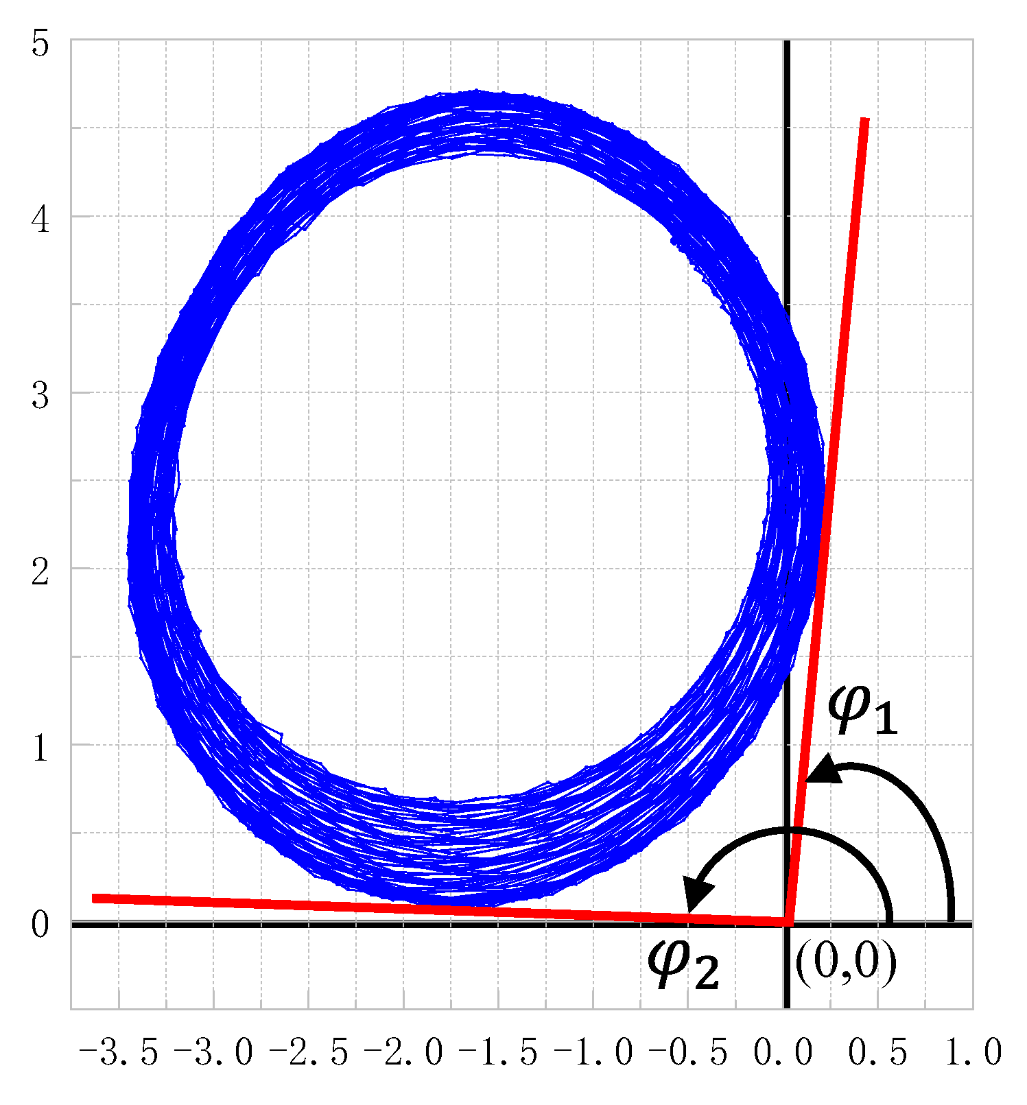
The maximum of the inequalities for ISM band are shown in Table 1. It can be seen from Table 1 that the maximum of the relative change rate of and occur in 2.45 GHz band. Take as the x-axis and as the y-axis. The simulated trajectory of this frequency band is investigated when and take the maximum value as shown in Figure 1. The similarity between the simulated trajectory and the fitting ellipse is very high. It is reasonable to regard the trajectory as an ellipse in the ISM band.
It can be seen from (15) and (16) that the greater the bandwidth, the greater the relative change rate of and , and the more the trajectory deviates from the ellipse. Due to the low bandwidth of ISM band, the trajectory can be regarded as an ellipse. If the changes of and are ignored under the condition of , and can be regarded as constants, denoted as and , respectively. In the actual environment, there will be various interferences, if only stationary objects are considered, the beat signal of stationary objects will be processed into DC offset based on (6) and (7), denoted as and , respectively. The DC offset will be added to and as shown in (17) and (18).
The trajectory equation is
Stationary objects do not affect the shape of the elliptical trajectory, they only affect the central coordinates of the ellipse. The ellipse parameters, that is, the value of , can be obtained by the ellipse fitting.
2.3. Principle of Motion Measurement
According to (17) and (18), the absolute unambiguous phase corresponding to the point on the elliptical trajectory is:
After obtaining the parameters of the fitted ellipse, the tangent of the phase can be obtained as:
Arctangent function is not a single valued function. Generally, the single value range is limited to 2π. So, the angle obtained by the arctangent function is not necessarily equal to .
The problem that the range of is limited to 2π can be solved by the phase unwrapping algorithm.
and denote and of the m-th sampling chirp, denote of the m-th sampling arctangent phase, and the is:
Generally, the range of arctangent function obtained by computer is (, which can be extended to by (24).
The m-th unwrapping phase is:
is the relative index of the unwrapped phase, for the first value, . The process of unwrapping is to determine . The phase jumps when it enters the adjacent interval and the index should increase or decrease by one. Whether the phase jumps can be determined by the difference between the current phase and the previous phase.
Since the initial unambiguous phase is unknown, what we get is a relatively unambiguous phase. From the relative phase, the displacement of the m-th sampling chirp is:
The ellipse approximation algorithm also provides an estimation method of the distance from the target to the antenna. Movement distance of can just make the trajectory of and form a complete ellipse, it can be seen from (6), (7), (17), and (18) that the long and short axes of the ellipse satisfy (28).
Equation (29) provides a way for estimating the distance R by the parameters of the fitting ellipse. and are the parameters of the fitting ellipse when the target has a displacement not greater than . Ideally, the distance estimated by Equation (29) is an average value in the movement, and the accuracy should not be greater than . However, the actual measurement accuracy cannot reach the ideal situation because it will be affected by the nonlinearity of the transmitting wave, signal-to-noise ratio, accuracy of ellipse fitting, etc. In the experiment part, the measurement accuracy under the given experimental setup will be shown.
Sometimes the initial distance, , of the object relative to the radar is known, for example, in the measurement of vital signs, the position of the people is determined in advance. In this case, the initial discrete frequency number can be obtained by according to (9), the symbol indicates rounding the value inside. The value of is not large for low bandwidth, e.g., when the bandwidth is 0.15 GHz, the distance of 5 m corresponds to = 5. If the value of is unknown, one simple way is to test the appropriate by changing it manually. The general way to obtain is signal processing. The distance, , can be estimated by the frequency estimation method in [10,11,12,13,14] for the first chirp, and then calculate . The values of can be updated by , where is the displacement of the m-th sampling chirp.
Some details of the algorithm are presented in Appendix A, and a flowchart of the whole algorithm is given in Appendix B.
3. Measurement Results
3.1. Measurement Setup and the Shape of Trajectories
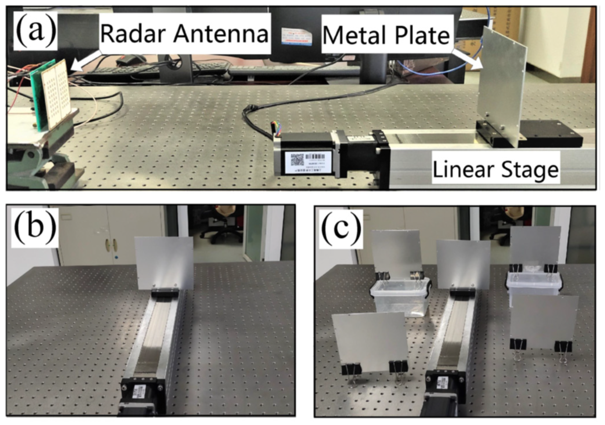
Commercial chip solutions are now available for key radar components, which greatly simplifies the design and manufacturing of small radar systems. In this experiment, the radar system is mainly composed of ADI’s ADF4158 chip and Infineon’s BGT24MTR chip. The ADF4158 chip generates the modulated signal; the BGT24MTR chip includes a 24 GHz voltage-controlled oscillator (VCO), a 24 GHz Mixer, a 24 GHz radio frequency power amplifier (PA) and a 24 GHz low noise amplifier (LNA). The two chips constitute the waveform generator. The digital acquisition (DAQ) card of Ni’s PXI-4461 is used for signal acquisition, and the digital signal analysis is completed by the embedded controller of NI’s PXI-8101. The embedded controller acts as a computer, which includes a CPU of Intel Celeron 575 and 1 Gb RAM. The software used for signal acquisition is LabVIEW and the software of signal processing is MATLAB. The DAQ card and the embedded controller are installed in the chassis of NI’s PXI-1036. The above devices are shown in Figure 2.
A metal plate is fixed on the linear stage as the object to be measured. The moving direction of the linear stage is perpendicular to the antenna of the radar. The measurement setup is shown in Figure 3 and the specifications are shown in Table 2.
As mentioned before, stationary objects do not affect the shape but the center point of the ellipse. In order to verify this hypothesis, some experiments were carried out in the environments shown in Figure 3b,c.
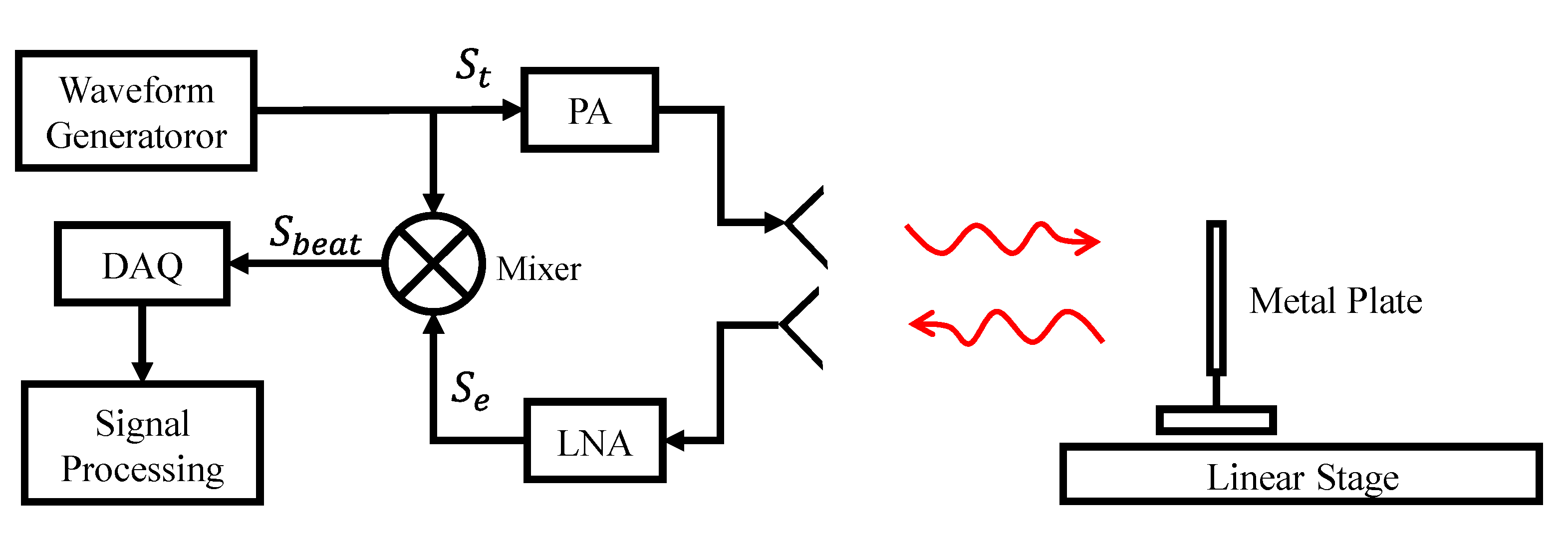
The block diagram of the measurement system is show in Figure 4. The FMCW signal produced by the waveform generator is amplified by the PA and transmitted to the metal plate. The echo is amplified and filtered by the LNA, and mixed with a part of the transmitted signal to generate the beat signal, which is then converted into a digital signal through DAQ card and processed by the computer.
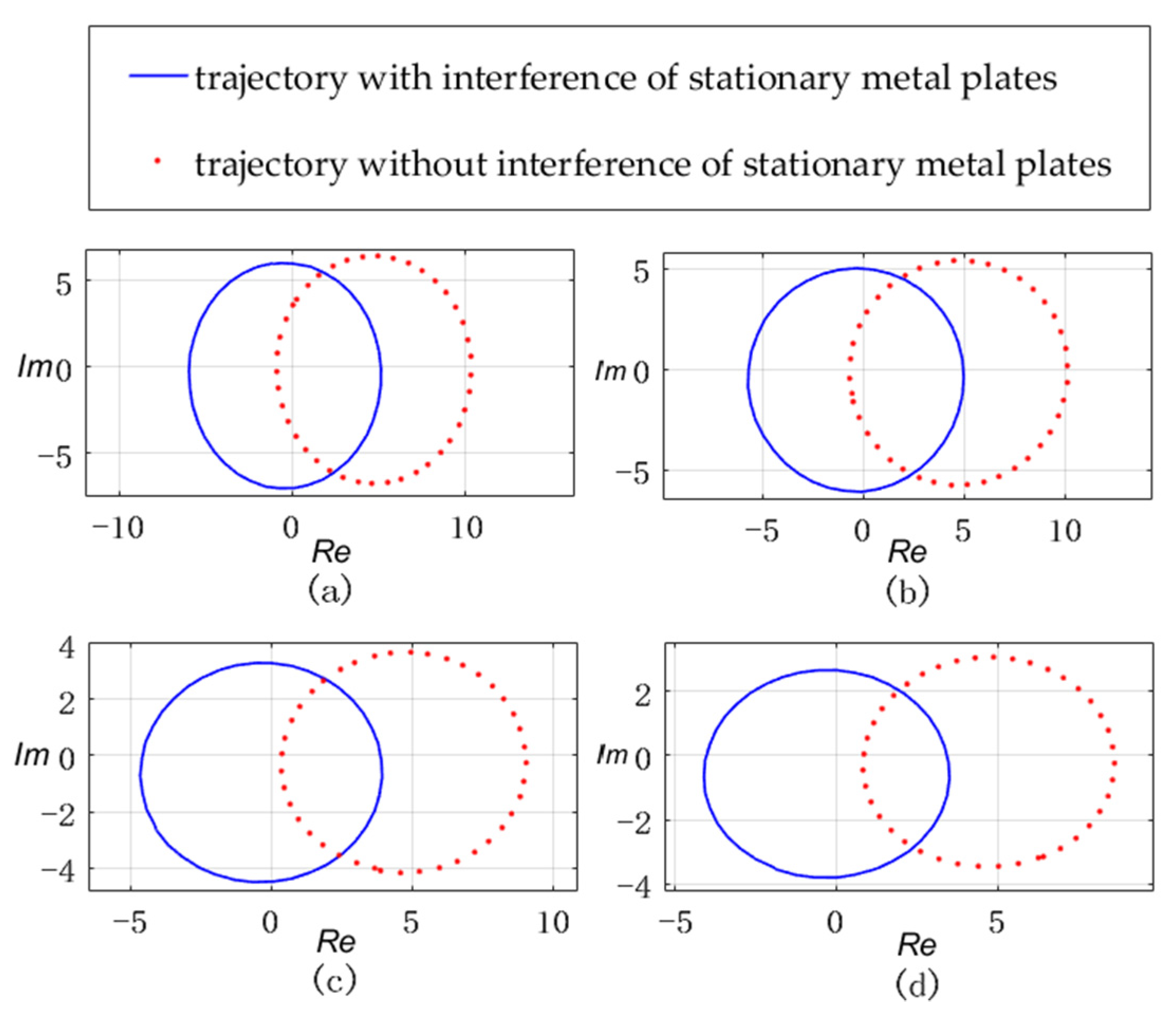
Let the metal plate move by at 1.7 m, 1.9 m, 2.1 m, and 2.2 m away from the antenna, respectively. The synthetic trajectory of and is shown in Figure 5. The trajectory composed of solid lines represents the measurement results without stationary metal plates and the trajectory composed of dots represents the results with stationary metal plates. It can be seen that the trajectory is indeed in the shape of an ellipse. Two trajectories composed of solid lines and dots in each subgraph have the same shape but have a different position, which is consistent with the previous hypothesis.
3.2. Motion Measurement
In order to test the accuracy of the proposed algorithm in motion measurement, the following movement process is designed: first, start moving at an acceleration of 5 mm/s2 for 4 s from a standstill, the speed will reach 20 mm/s, move at this speed for 10 s, then move at an acceleration of—5 mm/s2 for 4 s, and at this time, the speed is zero; stand still for 2 s, then move at an acceleration of—10 mm/s2 for 2 s, the speed reaches—20 mm/s, and then move at this speed for 12 s. Lastly, move at an acceleration of 10 mm/s for 2 s and return to the starting point. The whole movement can be divided into seven motion states as shown in Table 3.
The sampling rate of displacement is 65 Hz, and the movement lasts for 36 s; there are 2340 sampling values in a complete measurement. The complete measurement was repeated 50 times in the two environments as shown in Figure 3b,c, which means there are 50 values in every position during movement. Figure 6 shows the statistical analysis of deviation between the measured value and the set value. The blue line represents the change of the maximum absolute measurement deviation, the red line represents the change of standard deviation. In Figure 6a, the maximum value of the blue line is 0.087 mm, the maximum value of the red line is 0.036 mm. In Figure 6b, the maximum value is 0.082 mm for the blue line and 0.037 mm for the red line. In both environments, the measurement has reached sub-millimeter accuracy. Considering that the positioning accuracy of the linear stage is 0.01 mm, there is no obvious difference in measurement deviation in the two environments. It is reasonable to consider that the algorithm can filter the interference of the stationary object.
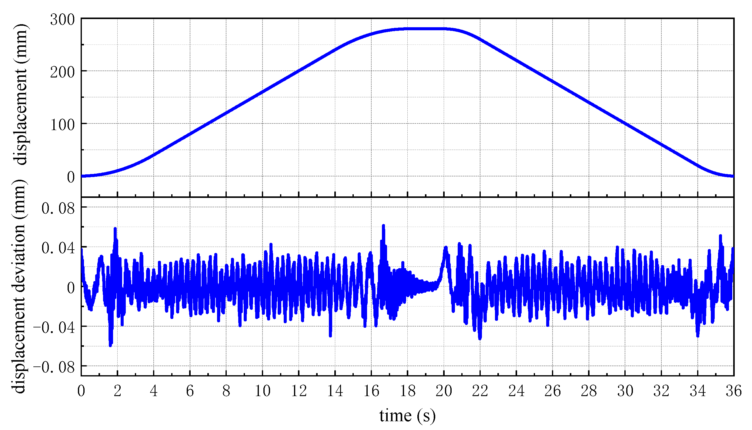
Figure 7 shows one measurement result randomly selected from 50 measurements without interference of stationary metal plates; the upper figure shows the measured displacement, and the lower figure shows the deviation between the measured value and the set value. The maximum value of displacement deviation is 0.061 mm. It can be seen that the deviation is large in the acceleration period, smaller in uniform in the velocity period, and is the smallest in the standstill period. The reason is that the metal plate is fixed on the slider of the linear stage, and when the linear stage drives the metal plate to move, it vibrates slightly and transfers this vibration to the metal plate resulting in additional deviation. Accelerated motion causes a stronger vibration than uniform motion, so the deviation in acceleration period is larger than that of uniform velocity and the standstill period.
If the conventional phase evaluation method is adopted, which means the phase is evaluated by (8), the displacement deviations for a complete measurement with/without interference of stationary metal plates are shown in Figure 8. The maximum value of absolute deviation is 1.127 mm and 0.722 mm for Figure 8a,b, respectively. The deviation is about ten times that of the phase correction algorithm.
According to (8), the unequal of and does not change the quadrant of the phase, the maximum deviation of phase caused by it satisfies , and the maximum displacement deviation satisfies . For this experiment, = 12.461 mm, so < 1.558 mm. The above measurement results agree with the theory.
The conventional phase evaluation method is more vulnerable to DC offset. There is an extreme case that the DC offset makes the coordinate origin outside the trajectory, which distorts the quadrant of the phase and makes the phase impossible to estimate correctly. This case is achieved by placing the stationary metal plate in a specific position, and the motion measurement is carried out under the condition. The coordinate origin is outside the trajectory as shown in Figure 9. For conventional phase evaluation method, the phase range is limited to , so the displacement is limited to less than half a wavelength, resulting in a huge measurement deviation that it is completely wrong as shown in Figure 10a. The results calculated by the ellipse approximation algorithm are shown in Figure 10b, and compared with Figure 7, it can be seen that the accuracy of the measurement is not affected by the origin position for the ellipse approximation algorithm.
The performance of other works is shown in Table 4. It can be seen that the measurement accuracy of [16,22,23], is higher than this work. In [22], the measured distance is only 0.01 mm, it is applicable to the ultra-short distance measurement. Ref. [16] uses a complex frequency estimation algorithm based on chirp Z-transform. The experiment was carried out in a special measurement environment with a closed setup and no external influences, which cannot reflect the anti-interference ability. Ref. [23] uses a phase modulated radar which has an advantage in that multiple sensors could coexist without interference with each other; however, in the experiment, the target is measured at several fixed positions, the performance of motion measurement is not given, and the frequency band does not belong to ISM band.
The time complexity represented by big O notation is given in Table 4. Big O notation can tell us how efficient the algorithm is. It can be seen that the time complexity of [22,24] is a constant order of O(1). For the CW radar, if the DC offset is not considered, the arctangent demodulation can be directly used on the echo signals of the IQ channel, which has a fast response speed, but the measurement results are very sensitive to the noise. The signal processing of FMCW radar generally has an integral for the beat signal, and compared with the CW radar, the response speed is slower, but the integration can effectively eliminate random noise. The time complexity of the algorithm in this paper is consistent with [23,25], and better than [10,16].
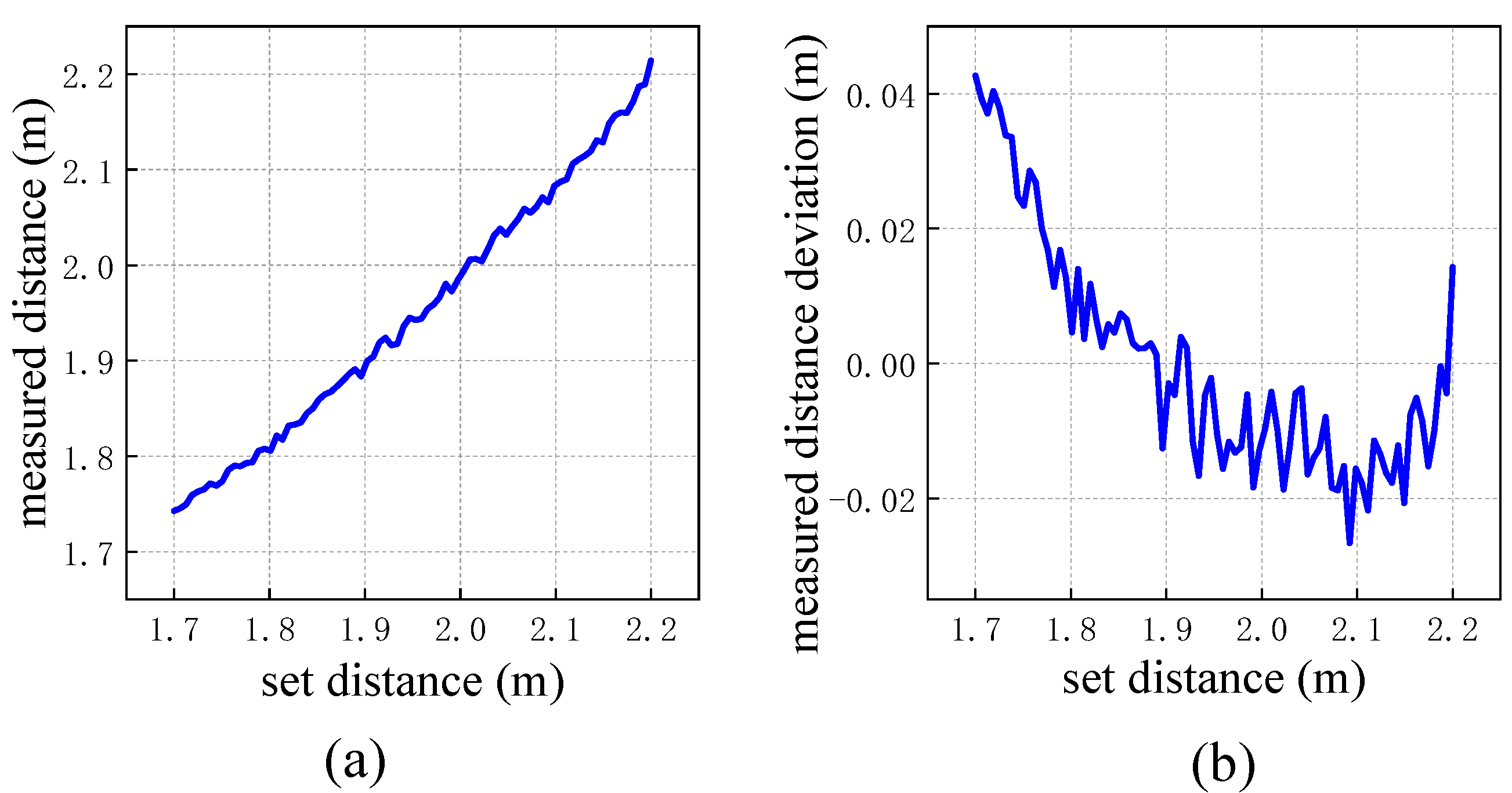
3.3. Distance Measurement
The distance between the target and the antenna can be calculated according to (20). Let the linear stage carrying the metal plate move 0.5 m, and the initial distance from the antenna is 1.7 m. Since the measurement results with or without the stationary metal plate are almost the same, only the measurement results without the stationary metal plate are given, as shown in Figure 11.
The x-axis of Figure 11a represents the set distance and the y-axis represents the measured distance. The curve of Figure 11a would be a straight line if there are no measurement deviations. It can be seen that the maximum deviation is 0.043 m as shown in Figure 11b. The accuracy of the distance measurement is not high, but the computational complexity is low. Different scenarios have different requirements for measurement accuracy. For example, the obstacle avoidance of autonomous vehicles requires centimeter accuracy, and the motion detection of the robotic arm in remote surgery requires sub-millimeter accuracy. Meanwhile, real-time performance is another important consideration. Algorithms with high computational complexity require hardware with strong computational power, and cannot achieve a good balance between low latency and low cost. This algorithm can be used in scenes with low requirements for accuracy but high requirements for real-time performance, such as car reversing alarm, indoor robot obstacle avoidance, etc.
The linear stage we use is 50 cm long, and the experiment was carried out indoors. Due to space limitations, the maximum distance is 5 m and the maximum displacement is 50 cm in the measurement, and within this range, no significant change in accuracy was found. However, this does not mean that distance has little effect on accuracy. In general, the maximum measurement distance of the radar is proportional to the transmitted power and the object’s cross section, and inversely proportional to the noise; in other words, it is related to the signal-to-noise ratio (SNR). The increase in the distance will reduce the SNR and have a negative impact on the measurement accuracy, which must be paid attention to, especially for high accuracy measurement.
4. Discussion
High accuracy phase evaluation is the key to accurate motion detection. The conventional FFT phase algorithm has phase distortion due to spectrum leakage, and cannot eliminate DC offset. The frequency estimation method contains Fourier transform and frequency refining analysis in each chirp, which has the disadvantages of being computationally expensive, and easily disturbed by surrounding objects. In this paper, a more accurate phase estimation is presented for the ISM band. The algorithm only needs one receiving channel, and can eliminate the DC offset.
The proposed algorithm can obtain accurate movement displacement, and can be applied to scenes where the relative motion needs to be measured remotely and non-contact, such as life signal detection, robot control, etc. However, the accuracy of absolute distance is low. The approach to solve this problem can be combined with the frequency estimation method in [7,16]. There is no need to complete frequency estimation for each chirp. Instead, just calculate the accurate distance for the first chirp, and then use the sum of the displacement and the initial distance to obtain the accurate distance.
The proposed algorithm can eliminate the DC offset caused by a stationary object, no matter whether the stationary object is close or far away from the target. If there is interference from a moving object, the situation is more complicated. If the distance between the moving object and the target is greater than a range bin of FMCW radar, the frequency difference between their beat signals is greater than the discrete frequency interval of DFT, and the two motions can be distinguished because of the weak correlation between their beat signals; if the distance is less than a range bin, it is difficult to distinguish the two motions because of the strong correlation of their beat signals. It is an effective method to increase the range resolution by increasing the bandwidth, but it is not suitable for the ISM band because its bandwidth range is very limited. If the two moving objects do not block each other, they will be at different angles to the receiving antenna. Increasing the number of receiving antennas can improve the ability of azimuth resolution, which is a way to distinguish different moving objects.
5. Conclusions
The proposed algorithm to calculate displacement by accurate phase avoids the use of complex methods for frequency estimation and reduces the amount of calculation. Since the beat signal of the stationary object is processed into a fixed DC offset, the interference of the stationary object can be filtered, which reduces the requirements for the measurement environment. This algorithm is especially suitable for ISM band, so it has high practicability. The performance of the algorithm is evaluated by a radar system which the center frequency is 24.075 GHz and the bandwidth is 0.15 GHz; the measurement accuracy of displacement is 0.087 mm and the accuracy of distance is 0.043 m.
Author Contributions
Conceptualization, R.Z. and K.Q.; methodology, K.Q.; software, K.Q.; validation, K.Q. and R.Z.; formal analysis, K.Q.; investigation, K.Q.; resources, R.Z.; data curation, K.Q.; writing—original draft preparation, K.Q.; writing—review and editing, K.Q. and Z.F.; supervision, R.Z. and Z.F.; and funding acquisition, R.Z. All authors have read and agreed to the published version of the manuscript.
Funding
This research was funded by the National Key Scientific Instrument and Equipment Development Project of China, grant number 2016YFF0101402.
Institutional Review Board Statement
Not applicable.
Informed Consent Statement
Not applicable.
Data Availability Statement
The data presented in this study are available on request from the corresponding author.
Conflicts of Interest
The authors declare no conflict of interest.
Appendix A
In the following description, the sampling point coordinates of the elliptical trajectory are the values of each pair of and . Some sampling points are selected for ellipse fitting, and these selected sampling points are called effective sampling points. The sampling points and the effective sampling points are stored as different variables.
- (1)
- The fitting of the initial ellipse
Noise will cause the sampling points formed by and to be randomly distributed in a small range, and the Euclidean distance between the sampling points is also randomly distributed. The distribution variance of the Euclidean distance is obtained through statistical analysis, and then the variance or variance with coefficient is set as a threshold. When the Euclidean distance between the current sampling point and the previous sampling point exceeds the threshold, the current sampling point can be stored as an effective sampling point for ellipse fitting.
At the beginning, the ellipse has not been formed, and the phase cannot be calculated immediately. Therefore, it is necessary to accumulate effective sampling points to fit the initial ellipse. First, set a number , when the number of accumulated effective sampling points is equal to , then use these effective sampling points to fit the initial ellipse. The time taken for accumulating effective sampling points and fitting the initial ellipse constitutes the initial delay time. After the initial ellipse fitting is completed, the corresponding phase of each sampling point within the initial delay time is calculated and the displacements are obtained. As for the determination of , if the value is too large, the delay time will be longer, and the trajectory may contain multiple ellipses; if the value is too small, the trajectory may be a short arc, resulting in a fitting error. In the experiment of this paper, the , the accuracy is good, and the initial delay time is 1.5 s.
- (2)
- The fitting of subsequent ellipse
If the sampling points enter the adjacent ellipse, the same problem is faced, that is, the current ellipse has not been formed and the corresponding parameters cannot be obtained immediately. We can assume that the two adjacent ellipse trajectories are almost the same, so the phase of current sampling points can be calculated according to the parameters of the previous ellipse. At the same time, the effective sampling points in the current ellipse are stored, and once the sampling point enters the adjacent ellipse, these effective sampling points are immediately used to fit the ellipse whose parameters are used for the phase calculation of the ongoing sampling points. The above procedure is repeated over time.
- (3)
- Restriction on the number of effective sampling points
If the measured object vibrates periodically within a range of less than half a wavelength for a long time, the sampling points will move periodically on an ellipse for a long time too, and a large number of effective sampling points will be collected on the ellipse. The computational cost of ellipse fitting will increase significantly. The solution is to divide the ellipse into intervals according to the phase, and each phase interval is . The rule is that only one effective sampling point is stored in each phase interval. The maximum number of effective sampling points on an ellipse will not exceed . The value of determines the sampling density, a large value will increase the computational cost, while a too small value will lead to a large fitting error. In the experiment of this paper, , which shows a good balance between accuracy and computational cost.
- (4)
- Ellipse fitting algorithm
The ellipse parameters can be estimated based on a linear least square (LLS) method, which is the optimum method for solving linear unbiased estimators.
Expand (19) into the following form:
The ellipse parameters are replaced by new linear parameters as follows:
Then (A1) can be
Let
The new parameters can be estimated based on LLS method as follows:
The following fourth-order linear equations which expressed by a matrix equation can be obtained:
where is a vector containing unknown parameters, is a vectors of constant term. and denote the coordinate of i-th effective sampling points. Where is the total number of effective sampling points, obviously . is the coefficient matrix.
Since the value of and is affected by random noise, is a full rank matrix, (A6) has a solution. The parameters of fitting ellipse can be obtained according to (A8)
The computational cost mainly includes the calculation of the elements of matrices and solving the fourth-order linear equations.
In the experiment of this paper, the NI’s PXI-8101 controller is used for computation, the CPU of the controller is Intel Celeron 575, the clock rate is 2.0 GHz. Set = 100, a customized program of this algorithm written in MATLAB is used for signal processing. The consumption time of ellipse fitting was measured many times during the experiment, and the maximum consumption time is 0.012 s.
Appendix B
Figure A1.
The flowchart of the algorithm.

References
- Zhe, T.; Huang, L.; Wu, Q.; Zhang, J.; Pei, C.; Li, L. Inter-Vehicle Distance Estimation Method Based on Monocular Vision Using 3D Detection. IEEE Trans. Veh. Technol. 2020, 69, 4907–4919. [Google Scholar] [CrossRef]
- Chew, M.T.; Alam, F.; Legg, M.; Sen Gupta, G. Accurate Ultrasound Indoor Localization Using Spring-Relaxation Technique. Electronics 2021, 10, 1290. [Google Scholar] [CrossRef]
- Ma, L.F.; Li, Y.; Li, J.; Wang, C.; Wang, R.S.; Chapman, M.A. Mobile Laser Scanned Point-Clouds for Road Object Detection and Extraction: A Review. Remote Sens. 2018, 10, 1531. [Google Scholar] [CrossRef] [Green Version]
- Arab, H.; Dufour, S.; Moldovan, E.; Akyel, C.; Tatu, S.O. A 77-GHz Six-Port Sensor for Accurate Near-Field Displacement and Doppler Measurements. Sensors 2018, 18, 2565. [Google Scholar] [CrossRef] [PubMed] [Green Version]
- Lee, H.; Kim, B.H.; Park, J.K.; Yook, J.G. A Novel Vital-Sign Sensing Algorithm for Multiple Subjects Based on 24-GHz FMCW Doppler radar. Remote Sens. 2019, 11, 1237. [Google Scholar] [CrossRef] [Green Version]
- Duan, Z.; Liang, J. Non-Contact Detection of Vital Signs Using a UWB Radar Sensor. IEEE Access 2019, 7, 36888–36895. [Google Scholar] [CrossRef]
- Piotrowsky, L.; Jaeschke, T.; Kueppers, S.; Siska, J.; Pohl, N. Enabling High Accuracy Distance Measurements with FMCW Radar Sensors. IEEE Trans. Microw. Theory Tech. 2019, 67, 5360–5371. [Google Scholar] [CrossRef]
- Wang, G.C.; Gu, C.Z.; Inoue, T.; Li, C.Z. A Hybrid FMCW-Interferometry Radar for Indoor Precise Positioning and Versatile Life Activity Monitoring. IEEE Trans. Microw. Theory Tech. 2014, 62, 2812–2822. [Google Scholar] [CrossRef]
- Anghel, A.; Vasile, G.; Cacoveanu, R.; Ioana, C.; Ciochina, S. Short-Range Wideband FMCW Radar for Millimetric Dis-placement Measurements. IEEE Trans. Geosci. Remote Sens. 2014, 52, 5633–5642. [Google Scholar] [CrossRef] [Green Version]
- Bredendiek, C.; Pohl, N.; Jaeschke, T.; Thomas, S.; Aufinger, K.; Bilgic, A. A 24GHz Wideband Single-Channel SiGe Bipolar Transceiver Chip for Monostatic FMCW Radar Systems. In Proceedings of the 15th European Microwave Week—Space for Microwaves Conference Proceedings, Amsterdam, The Netherlands, 28 October–2 November 2012; pp. 309–312. [Google Scholar]
- Agrez, D. Weighted multipoint interpolated DFT to improve amplitude estimation of multifrequency signal. IEEE Trans. In-strum. Meas. 2002, 51, 287–292. [Google Scholar] [CrossRef]
- Guoqing, Q. High accuracy range estimation of FMCW level radar based on the phase of the zero-padded FFT. In Proceedings of the 7th International Conference on Signal Processing, Beijing, China, 31 August–4 September 2004; pp. 2078–2081. [Google Scholar]
- Jaeschke, T.; Bredendiek, C.; Kuppers, S.; Pohl, N. High-Precision D-Band FMCW-Radar Sensor Based on a Wideband Si-Ge-Transceiver MMIC. IEEE Trans. Microw. Theory Tech. 2014, 62, 3582–3597. [Google Scholar] [CrossRef]
- Luo, J.F.; Xie, Z.J.; Xie, M. Interpolated DFT algorithms with zero padding for classic windows. Mech. Syst. Signal Proc. 2016, 70–71, 1011–1025. [Google Scholar] [CrossRef]
- Rabiner, L.R.; Schafer, R.W.; Rader, C.M. The chirp z-transform algorithm and its application. Bell Syst. Tech. J. 1969, 48, 1249–1292. [Google Scholar] [CrossRef]
- Scherr, S.; Ayhan, S.; Fischbach, B.; Bhutani, A.; Pauli, M.; Zwick, T. An Efficient Frequency and Phase Estimation Algorithm with CRB Performance for FMCW Radar Applications. IEEE Trans. Instrum. Meas. 2015, 64, 1868–1875. [Google Scholar] [CrossRef]
- Scherr, S.; Goettel, B.; Ayhan, S.; Bhutani, A.; Pauli, M.; Winkler, W.; Scheytt, J.C.; Zwick, T. Miniaturized 122 GHz ISM Band FMCW Radar with Micrometer Accuracy. In Proceedings of the 12th European Radar Conference (EuRAD), Paris, France, 9–11 September 2015; pp. 277–280. [Google Scholar]
- Wang, S.Y.; Pohl, A.; Jaeschke, T.; Czaplik, M.; Kony, M.; Leonhardt, S.; Pohl, N. A Novel Ultra-Wideband 80 GHz FMCW Radar System for Contactless Monitoring of Vital Signs. In Proceedings of the 37th Annual International Conference of the IEEE-Engineering-in-Medicine-and-Biology-Society (EMBC), Milan, Italy, 25–29 August 2015; pp. 4978–4981. [Google Scholar]
- Radio Regulations Articles. Available online: https://www.itu.int/dms_pub/itu-r/opb/reg/R-REG-RR-2020-ZPF-E.zip (accessed on 28 October 2021).
- Li, C.Z.; Lin, J.S. Random Body Movement Cancellation in Doppler radar Vital Sign Detection. IEEE Trans. Microw. Theory Tech. 2008, 56, 3143–3152. [Google Scholar] [CrossRef]
- Zhao, H.; Hong, H.; Miao, D.Y.; Li, Y.S.; Zhang, H.T.; Zhang, Y.M.; Li, C.Z.; Zhu, X.H. A Noncontact Breathing Disorder Recognition System Using 2.4-GHZ Digital-IF Doppler radar. IEEE J. Biomed. Health Inform. 2019, 23, 208–217. [Google Scholar] [CrossRef] [PubMed]
- Barbon, F.; Vinci, G.; Lindner, S.; Weigel, R.; Koelpin, A. A six-port interferometer based micrometer-accuracy displacement and vibration measurement radar. In Proceedings of the 2012 IEEE/MTT-S International Microwave Symposium—MTT 2012, Montreal, QC, Canada, 17–22 June 2012. [Google Scholar] [CrossRef]
- Schlegel, A.; Ellison, S.M.; Nanzer, J.A. A Microwave Sensor with Submillimeter Range Accuracy Using Spectrally Sparse Signals. IEEE Microw. Wirel. Compon. Lett. 2020, 30, 120–123. [Google Scholar] [CrossRef]
- Lindner, S.; Barbon, F.; Mann, S.; Vinci, G.; Weigel, R.; Koelpin, A. Dual Tone Approach for Unambiguous Six-Port Based Interferometric Distance Measurements. In Proceedings of the 2013 IEEE MTT-S International Microwave Symposium Digest (MTT 2013), Seattle, WA, USA, 2–7 June 2013. [Google Scholar] [CrossRef]
- An, S.N.; He, Z.S.; Li, J.G.; An, J.P.; Zirath, H. Micrometer Accuracy Phase Modulated Radar for Distance Measurement and Monitoring. IEEE Sens. J. 2020, 20, 2919–2927. [Google Scholar] [CrossRef] [Green Version]
Figure 1.
Simulations of synthetic trajectory of and when = 2.45 GHz, = 0.1 GHz, k = 1,, and (a); (b).
Figure 1.
Simulations of synthetic trajectory of and when = 2.45 GHz, = 0.1 GHz, k = 1,, and (a); (b).

Figure 2.
(a) Power, radar, DAQ, and analysis devices. (b) Circuit containing key chips on the back of radar.
Figure 2.
(a) Power, radar, DAQ, and analysis devices. (b) Circuit containing key chips on the back of radar.

Figure 3.
(a) Measurement setup. (b) No stationary metal plates; (c) addition of stationary metal plates.
Figure 3.
(a) Measurement setup. (b) No stationary metal plates; (c) addition of stationary metal plates.

Figure 4.
Simplified block diagram of measurement system.

Figure 5.
The shape of synthetic trajectory with/without (solid blue/dashed red) interference of stationary metal plates, the change of R is , the starting distances are (a) 1.7 m; (b) 1.9 m; (c) 2.1 m; and (d) 2.2 m.
Figure 5.
The shape of synthetic trajectory with/without (solid blue/dashed red) interference of stationary metal plates, the change of R is , the starting distances are (a) 1.7 m; (b) 1.9 m; (c) 2.1 m; and (d) 2.2 m.

Figure 6.
The statistical analysis of measurement deviation. (a) With interference of stationary metal plates; and (b) without interference of stationary metal plates.
Figure 6.
The statistical analysis of measurement deviation. (a) With interference of stationary metal plates; and (b) without interference of stationary metal plates.

Figure 7.
Measured displacement (top) and the deviation (bottom) of ellipse approximation algorithm.
Figure 7.
Measured displacement (top) and the deviation (bottom) of ellipse approximation algorithm.

Figure 8.
Measurement deviation of conventional phase evaluation method. (a) With interference of stationary metal plates; (b) without interference of stationary metal plates.
Figure 8.
Measurement deviation of conventional phase evaluation method. (a) With interference of stationary metal plates; (b) without interference of stationary metal plates.

Figure 9.
The DC offset makes the coordinate origin be set outside of the trajectory by placing the stationary metal plate in a specific position. The phase range is limited to for the conventional phase evaluation method.
Figure 9.
The DC offset makes the coordinate origin be set outside of the trajectory by placing the stationary metal plate in a specific position. The phase range is limited to for the conventional phase evaluation method.

Figure 10.
The measured displacement (top) and the deviation (bottom) when the DC offset makes the coordinate origin outside the trajectory. (a) Conventional phase evaluation algorithm; (b) ellipse approximation algorithm.
Figure 10.
The measured displacement (top) and the deviation (bottom) when the DC offset makes the coordinate origin outside the trajectory. (a) Conventional phase evaluation algorithm; (b) ellipse approximation algorithm.

Figure 11.
Distance measurements of metal plate. (a) Measured distance versus set distance; and (b) the deviation of measured distance.
Figure 11.
Distance measurements of metal plate. (a) Measured distance versus set distance; and (b) the deviation of measured distance.


Table 1.
The maximum of the relative change rate of and for ISM band when .
| 0.00678 | 0.00003 | 1.47% | 1.06% |
| 0.01356 | 0.000014 | 0.34% | 0.25% |
| 0.02712 | 0.000326 | 4.01% | 2.88% |
| 0.04068 | 0.00004 | 0.33% | 0.24% |
| 0.43392 | 0.00174 | 1.34% | 0.96% |
| 0.915 | 0.026 | 9.47% | 6.82% |
| 2.45 | 0.1 | 13.61% | 9.80% |
| 5.8 | 0.15 | 8.62% | 6.21% |
| 24.125 | 0.25 | 3.45% | 2.49% |
| 61.25 | 0.5 | 2.72% | 1.96% |
| 122.5 | 1 | 2.72% | 1.96% |
| 245 | 2 | 2.72% | 1.96% |
Table 2.
Measuring setup specifications.
| Item | Parameter |
|---|---|
| Radar modulation mode | FMCW sawtooth modulation |
| Center frequency | 24.075 GHz |
| Bandwidth | 0.15 GHz |
| Duration of a chirp | 4 ms |
| Transmitted power | 15 dBm |
| Size of metal plate | 15 cm × 15 cm |
| Resolution of linear stage | 0.01 mm |
Table 3.
Motion state at different time periods of designed movement.
| Time Periods (s) | 0–4 | 4–14 | 14–18 | 18–20 | 20–22 | 22–34 | 34–36 |
|---|---|---|---|---|---|---|---|
| State of motion | Uniform acceleration | Uniform velocity | Uniform deceleration | standstill | Uniform acceleration | Uniform velocity | Uniform deceleration |
Table 4.
Comparison of performance with other works.
| Ref. | Waveform | Frequency(GHz) | Bandwidth (GHz) | Accuracy (um) | Measured Distance (mm) | Time Complexity | ISM Band |
|---|---|---|---|---|---|---|---|
| [10] | FMCW | 24 | 8 | 250 | 3000 | O() | NO |
| [16] | FMCW | 24.3 | 1 | 5 | 50 | O() | NO |
| [22] | CW | 24 | Single tone | 0.5 | 0.01 | O(1) | YES |
| [24] | CW | 24 | Dual tone | 200 | 60 | O(1) | NO |
| [25] | Pulse | 2 | 0.45 | 530 | Static | O(N) | NO |
| [23] | Phase modulated | 80 | 2 | 7 | 20 | O(N) | NO |
| This study | FMCW | 24.074 | 0.15 | 87 | 280 | O(N) | YES |
Publisher’s Note: MDPI stays neutral with regard to jurisdictional claims in published maps and institutional affiliations. |
© 2021 by the authors. Licensee MDPI, Basel, Switzerland. This article is an open access article distributed under the terms and conditions of the Creative Commons Attribution (CC BY) license (https://creativecommons.org/licenses/by/4.0/).
Share and Cite
MDPI and ACS Style
Qu, K.; Zhang, R.; Fang, Z. High Accuracy Motion Detection Algorithm via ISM Band FMCW Radar. Remote Sens. 2022, 14, 58. https://0-doi-org.brum.beds.ac.uk/10.3390/rs14010058
AMA Style
Qu K, Zhang R, Fang Z. High Accuracy Motion Detection Algorithm via ISM Band FMCW Radar. Remote Sensing. 2022; 14(1):58. https://0-doi-org.brum.beds.ac.uk/10.3390/rs14010058
Chicago/Turabian StyleQu, Kui, Rongfu Zhang, and Zhijun Fang. 2022. "High Accuracy Motion Detection Algorithm via ISM Band FMCW Radar" Remote Sensing 14, no. 1: 58. https://0-doi-org.brum.beds.ac.uk/10.3390/rs14010058
Note that from the first issue of 2016, this journal uses article numbers instead of page numbers. See further details here.