
A Comprehensive Clear-Sky Database for the Development of Land Surface Temperature Algorithms


1
Instituto Português do Mar e da Atmosfera (IPMA), 1749-077 Lisboa, Portugal
2
Instituto Dom Luiz (IDL), Faculdade de Ciências, Universidade de Lisboa, 1749-016 Lisboa, Portugal
*
Author to whom correspondence should be addressed.
Remote Sens. 2022, 14(10), 2329; https://0-doi-org.brum.beds.ac.uk/10.3390/rs14102329
Submission received: 15 February 2022
/
Revised: 25 March 2022
/
Accepted: 6 May 2022
/
Published: 11 May 2022
(This article belongs to the Special Issue Remote Sensing Monitoring of Land Surface Temperature (LST) II)
Abstract
:Land surface temperature is linked to a wide range of surface processes. Given the increased development of earth observation systems, a large effort has been put into advancing land surface temperature retrieval algorithms from remote sensors. Due to the very limited number of reliable in situ observations matching the spatial scales of satellite observations, algorithm development relies on synthetic databases, which then constitute a crucial part of algorithm development. Here we provide a database of atmospheric profiles and respective surface conditions that can be used to train and verify algorithms for land surface temperature retrieval, including machine learning techniques. The database was built from ERA5 data resampled through a dissimilarity criterion applied to the temperature and specific humidity profiles. This criterion aims to obtain regular distributions of these variables, ensuring a good representation of all atmospheric conditions. The corresponding vertical profiles of ozone and relevant surface and vertically integrated variables are also included in the dataset. Information on the surface conditions (i.e., temperature and emissivity) was complemented with data from a wide array of satellite products, enabling a more realistic surface representation. The dataset is freely available online at Zenodo.
1. Introduction
The surface processes are intrinsically linked to land surface temperature (LST), as it is a fundamental parameter of the surface energy balance [1,2,3,4,5]. Consequently, LST has been recently recognized as an Essential Climate Variable (ECV) [6] by the Global Climate Observing System (GCOS) program. Satellite observations remain the most effective method to obtain LST at multiple temporal and spatial resolutions [7]. For that reason, satellite-based LST has been increasingly used in a wide range of applications, such as the assessment of land surface schemes in numerical weather prediction models [8,9,10], monitoring of vegetation health [11,12], and extreme events [13,14], estimation of evapotranspiration [15,16,17], monitoring landcover change and urban heat islands [18,19,20,21,22], and climate studies [23,24,25], amongst others.
Over the last decades, a wide array of methods have been developed to retrieve LST, mostly from thermal infrared (TIR) imagery [7]. Despite the numerous retrieval algorithms available today, the training datasets used to calibrate those algorithms are very heterogeneous. As reliable in situ observations that represent the satellite scale are very limited, these training datasets generally rely on top-of-atmosphere (TOA) radiances obtained from a radiative transfer model. These models take as input a variety of atmospheric profiles and surface properties that are considered to be representative of a range of possible atmospheric and surface conditions. The sampling of those profiles has been performed with very different methodologies and data sources, for instance: the Satellite Application Facility on Land Surface Analysis (LSA-SAF) has used a combination of atmospheric profiles from the European Centre for Medium-Range Forecast (ECMWF) 40-year reanalysis (ERA-40) and from clear-sky radiosondes [26] gathered by Borbas et al. [27]; the algorithm for the MODerate resolution Imaging Spectroradiometer (MODIS) LST product MYD11/MOD11 was calibrated using 12 temperature profiles and re-scaled water vapor profiles [28], while product MYD21/MOD21 also used the database compiled by Borbas et al. [29]; conversely, the Along-Track Scanning Radiometer (ATSR) LST algorithm was trained using a random selection of ECMWF ERA-Interim reanalysis with forced uniform spatial and temporal coverage [30]; the Copernicus Global Land Service (C-GLOPS) considers a subset of profiles from the dataset gathered by Borbas at al., where the selected profiles follow uniform distributions of water vapor and skin temperature [31]. The methodologies used to define the surface temperature and emissivity used in algorithm calibration are even more heterogeneous; assigned surface temperatures range from model estimates, empirical relationships between surface air and skin temperatures, or simple fixed temperature intervals centered at values typically observed in stations.
Most LST products derived from satellite observations rely on (semi-)empirical models fitted to a calibration dataset. Despite the importance of such a calibration database for the overall performance of the final model, little attention is generally given to the selection criteria of the cases (i.e., the atmospheric profiles) and distributions of the corresponding variables. The impact the training data may have on the robustness of the parameters of these mathematical models is not negligible and could compromise their quality. In particular, the training dataset should represent a wide range of surface and atmospheric conditions, frequently observed or not, to ensure a global good performance.
The topic of building a representative database of a priori information has been addressed in the past, mostly in the context of the retrieval of atmospheric profiles from satellite data. The first major attempt to build a global-scale database of atmospheric profiles for modeling forward and inverse radiative transfer problems has been the development of the multiple versions of the Thermodynamic Initial Guess Retrieval database (TIGR) [32,33,34,35,36]. These databases were built from radiosonde data, applying a dissimilarity criterion based on the temperature to obtain regular distributions. The National Oceanic and Atmospheric Administration (NOAA) also compiled a dataset of radiosondes, the NOAA-88. This dataset encompassed 7547 globally distributed clear-sky profiles of water vapor, temperature, and ozone, together with observations of surface pressure and near-surface air temperature. The dataset was complemented with radiosonde data from the Sahara region to circumvent the lack of data for very warm surfaces [37].
Complementary to observation-based databases, Chevallier proposed the use of numerical weather prediction data to build profile databases from the 31- and 50-layer ECMWF short-range forecasts [38] and later from the 60-level ECMWF 40-year reanalysis (ERA-40) [39]. These datasets based on numerical weather prediction models had the advantage of providing a large set of surface and profile variables that are consistent with each other and available at full spatial and temporal coverage. The sampling strategy of these datasets was similar to the TIGR, using a dissimilarity criterion simultaneously applied to temperature and specific humidity profiles. The recent version 12 of the Radiative Transfer for TOVS (RTTOV) fast radiative transfer model [40] used a training database of atmospheric profiles from the ECMWF ERA-Interim reanalysis [41]. In this case, the temperature, specific humidity, ozone, cloud condensation, and precipitation datasets were built independently using the same approach as Chevallier et al. [38]. This database was developed as a result of the ECMWF work on cloud and precipitation to improve the distribution of each individual variable. Aires and Prigent [42] also explored a clustering technique to resample the ERA40 database for the calibration of statistical retrieval algorithms. The purpose of using this technique was to reproduce the original distributions of the database with the sampling method. Conversely, Mattar et al. [43] built a training database from ERA-Interim profiles selected based on the type of climate, spatial location, water vapor content, and temporality.
Borbas et al. [27] combined the data from NOAA-88, TIGR-3, and ERA-40 together with radiosondes from 2004 in the Sahara Desert into a single training database. The so-called SeeBor database is currently the most widely used in LST retrieval and has been used as a benchmark for calibrating multiple remote sensing LST products [44,45,46,47,48,49,50,51,52,53].
However, the profile data used in the SeeBor database is significantly outdated. In particular, the most recent ECMWF version-5 reanalysis (ERA5) [54] is now available, providing atmospheric profiles on 137 levels, with a much more detailed representation of atmospheric conditions close to the surface and with hourly frequency, allowing getting profiles more representative of the whole diurnal cycle, when compared with the previous 6-hourly reanalysis. The higher spatial resolution (30 km) and improved surface scheme used in ERA5 also lead to a much more realistic surface temperature when compared with ERA-40. We consider that the use of reanalysis data is the most appropriate strategy to build a calibration database for LST algorithms since it combines large amounts of historical observations (including radiosondes) using the most advanced modeling and data assimilation systems while providing full spatial and temporal coverage. Additionally, the new ERA5 reanalysis shows a better agreement (compared to the older ERA-Interim) to observations over the entire troposphere, particularly for the near-surface parameters [54]. Since most of the TIR signal originates from the lower troposphere, it has the potential to provide a better reference for TIR-based retrievals when compared with ERA-Interim and is significantly better than the ERA-40 profiles used in SeeBor.
We propose building a comprehensive clear-sky database for TIR-based LST retrieval from ERA5 data using the sampling methodology proposed by Chevallier et al. [38]. In the TIR domain, temperature and specific humidity are the most relevant variables for LST retrieval, making this sampling method particularly appropriate. Moreover, this type of sampling methodology is preferred here as it allows obtaining uniform distributions of the temperature and specific humidity profiles; sampling methods based on uniform distributions in time and space are more likely to lead to irregular distributions of these variables due to physical constraints [38,55]. The surface conditions are defined from the combined use of ERA5 and satellite data to increase the database’s representativeness. For reference, we compare the different variable distributions of the new database with those of SeeBor, since it includes a wide range of the datasets previously mentioned.
2. Materials and Methods
2.1. Model Data
The calibration database is built using data from the ECMWF reanalysis ERA5. ERA5 provides hourly estimates of numerous atmospheric, land, and oceanic climate variables. Three main subsets of variables were used, namely:
- Atmospheric profiles, including temperature, specific humidity, and ozone on model levels (137 levels from the surface up to a height of 80 km).
- Surface variables, including 2-m temperature (T2 m), surface pressure (SP), skin temperature (Tskin), land-sea mask, geopotential, and the logarithm of surface pressure (the last two are used to obtain the height and pressure of each model level).
- Vertically integrated or column variables, namely total column water vapor (TCWV) and total cloud cover (TCC).
All data correspond to hourly data (24-time slots) for the 15th day of each month within the 2009–2019 period, interpolated to a 1° × 1° spatial grid. Only land and clear-sky conditions are considered by limiting TCC to values below 30%.
Surface and atmospheric column variables were also downloaded from the ERA5 archive with a resolution of 0.25° × 0.25° for all times-of-day and all days within the 2018–2020 period. As further detailed below, this last group of data will be used in combination with satellite data to examine and define the surface conditions that should be considered when building the calibration database.
2.2. Satellite Data
Satellite-based LST and surface emissivity are used here in combinationwith the ERA5 data to define the surface conditions for the training database. To reduce the impact of sensor-specific biases and increase spatial and temporal coverage, we consider various LST products, namely: the LSA-SAF LST products derived from the Spinning Enhanced Visible and Infrared Imager (SEVIRI) onboard the European series of Meteosat Second Generation (MSG) satellites, including the Indian Ocean Data Coverage (IODC), and from the Advanced Very High-Resolution Radiometer (AVHRR) onboard the European series of polar-orbiter satellites, Metop [26,56]; the C-GLOPS LST product based on the Advance Baseline Imager (ABI) onboard the Geostationary Operational Environmental Satellites-R Series (GOES-R) and on the Advanced Himawari Imager (AHI) onboard the Himawari series (https://land.copernicus.eu/global/products/lst accessed on 26 May 2021). The MSG (GOES-R and Himawari) products are available with a temporal sampling of 15 (10) min and a spatial resolution of 3 km (2 km) at the sub-satellite point. The AVHRR product has a spatial resolution of about 1 km and is available approximately twice daily at 9:30 and 21:30 local time.
All the above-mentioned LST products are based on the Vegetation Cover Method (VCM) for a priori emissivity estimation [57], using the respective Fraction of Vegetation Cover (FVC) products produced by the LSA-SAF and C-GLOPS. These emissivity datasets are available internally at the LSA-SAF with the same spatial resolution as the LST products and a daily temporal sampling.
To further increase the range of possible emissivity values, we further include data from the MODIS Temperature Emissivity Separation (TES) algorithm, which provides direct retrievals of emissivity in the TIR spectral range (MYD21C1) [58]. The MYD21C1 product provides daily day/night composites of LST and emissivity for MODIS bands 29, 31, and 32 on a 0.05° × 0.05° grid.
All datasets are projected onto the ERA5 0.25° × 0.25° grid by a simple average of all pixels within each grid box. For the geostationary satellites, only the LST retrievals with reference times of 00, 01, …, 22, 23 UTC were used to match the hourly sample of ERA5. For AVHRR LST, all observations within ± 15 min of the ERA5 hourly data were considered.
2.3. Profile Selection Methodology
We aim to build a training database consisting of a subset of ERA5 variables fully representative of all possible atmospheric and surface conditions in the original database.
To ensure that all climate conditions are considered in the database, we start by defining classes of TCWV varying from 0 to 60 mm in steps of 5 mm (with the last class also encompassing values above 60 mm), and classes of Tskin varying from 190 to 350 K in steps of 10 K. We recall that only “clear-sky” cases, i.e., profiles with TCC below 30%, are considered; the “30%” threshold is a compromise between ensuring the use of ERA5 clear-sky profiles, while still maintaining a reasonable pool of data to build our database. The TCWV is used here to stratify the database in terms of bulk atmospheric conditions since the variability of the TCWV is much more heterogeneous than that of the temperature and tends to increase with increasing TCWV value. Then, the Tskin stratification is incorporated to ensure all surface conditions are considered for each TCWV range (for instance, very dry atmospheres may occur over deserts and snow-covered regions with very different surface temperature ranges).
Then, for each class of TCWV and Tskin, approximately 1000 profiles are selected using the methodology of Chevallier et al. [38]. Chevallier et al. use an iterative process to select a subset of profiles from the initial database based on the dissimilarity between the profiles. The proximity criterion is considered in the temperature and specific humidity spaces separately and is measured through the non-Euclidian distances:
where and are the temperatures and specific humidity at levels and represent two atmospheric profiles from the database. () is the standard deviation of () computed from the original database for the selected class of TCWV and Tskin. The selection is performed as follows:
- For a given TCWV and Tskin class, a pair of profiles of and is randomly selected from the original database and put in the calibration database.
- A new pair of profiles is then selected randomly from the original database. The distances and are calculated between the new profiles and each pair of profiles already in the calibration database. The minimum values, and , are then computed.
- The new pair of profiles are stored in the database if and meet the threshold criteria for the minimum acceptable distance:
The parameter is introduced to account for the difference in vertical variability of the two variables and takes a value of 1.9, following Chevallier et al. [38].
- 4.
- Steps 2 and 3 are repeated until all profiles in the original database have been tested.
Higher values limit the database to higher distances, and , between profiles, i.e., only profiles with higher dissimilarity are selected. However, the values of and also depend on the distribution of and in the original database. Consequently, the value of must be updated for each TCWV and Tskin class in order to reach the desired sample size (in this case, 1000, with an allowance of ±10 profiles to simplify the calculations). For that purpose, values are adjusted iteratively: first, a random is selected, and the profiles’ selection process (steps 1–4) is performed; if the resulting sample size is higher/lower than the target, then is increased/decreased; this process is repeated until the desired sample size is achieved.
The sampling is performed on model levels to achieve higher accuracy (avoiding vertical interpolation to pressure levels) and to encompass a wide range of atmospheric conditions, including high elevated ground [38]. Figure 1 shows the sample size of each class of the original and calibration databases. For some classes, the number of available profiles in the original database is below the 1000 target, in which case all available profiles are used.
3. Results
3.1. Spatial Distribution
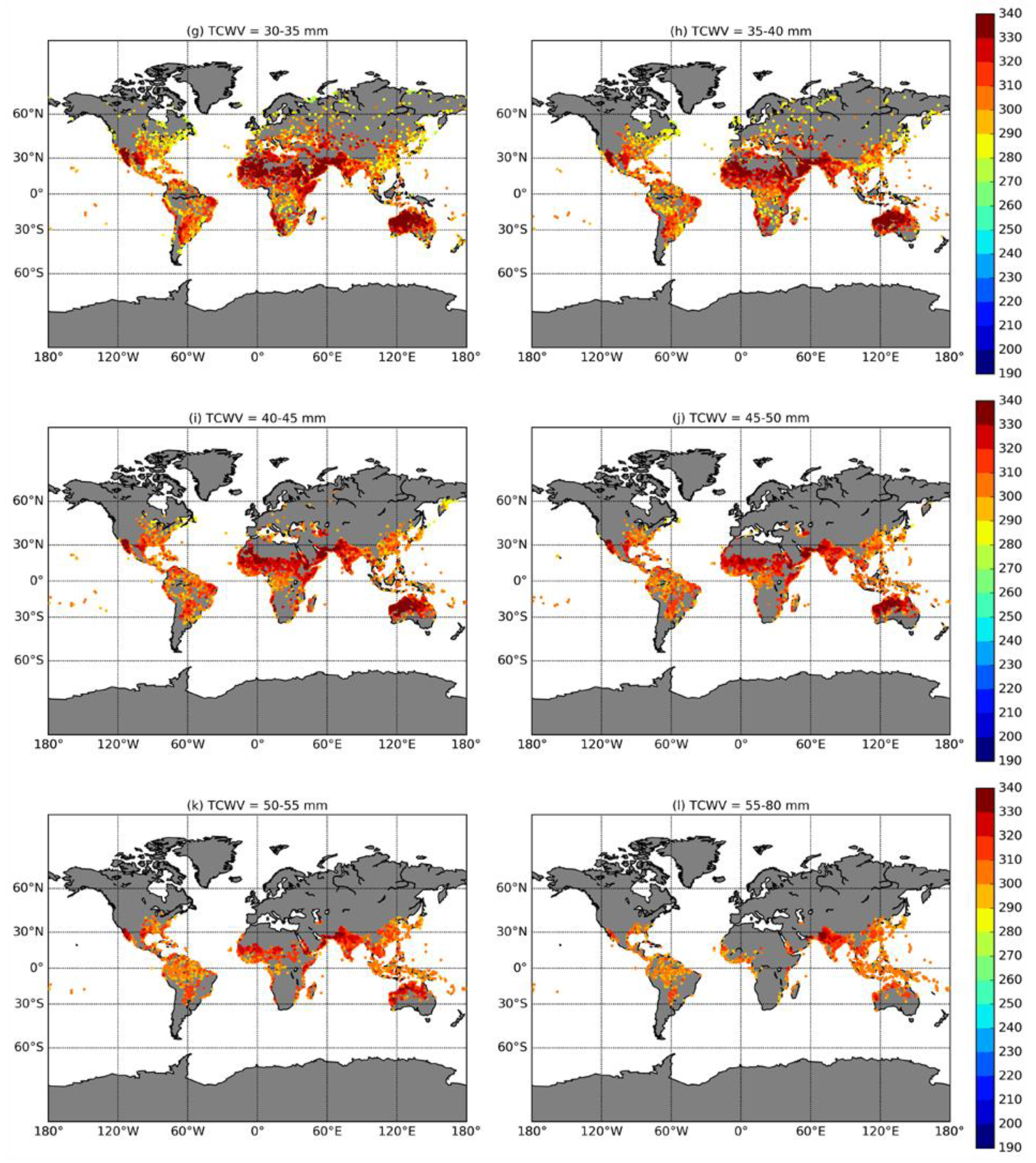
Figure 2 shows the geographical distribution of the profiles selected for the database. As expected, the availability of data is constrained by the local climate, and therefore some regions cannot be represented for some classes of TCWV and Tskin.
It is also expected that some regions of the planet might have higher variability of atmospheric and surface conditions, which means that some locations may have a higher representation in the database (e.g., dry or semi-arid regions). Nevertheless, constructing this database aims to ensure that all possible atmospheric/surface conditions are represented, which can only be achieved by including a large number of profiles over some regions.
3.2. Temporal Distribution
In the original dataset, the full diurnal cycle of each day is included in order to incorporate a higher variability of atmospheric conditions. Naturally, the sampling method described above will condition the temporal distribution of the data. Figure 3 shows the distribution of local time and of the months of the profiles sampled for each TCWV class. The sampling tends to be uniform during the night and has increased values towards noon. Likely, there is a higher variability of atmospheric conditions, particularly for temperature, during these times of the day. There is also a higher frequency of values during the northern hemisphere summer months (June to August) for the classes of higher TCWV. This is because very moist atmospheres can only occur under warmer temperatures (as depicted in Figure 1). Given the much larger land area in the northern hemisphere, the histogram shows higher frequencies for the northern hemisphere summer. Nevertheless, the sampling is representative of all times of day and all seasons.
3.3. Vertical Distribution
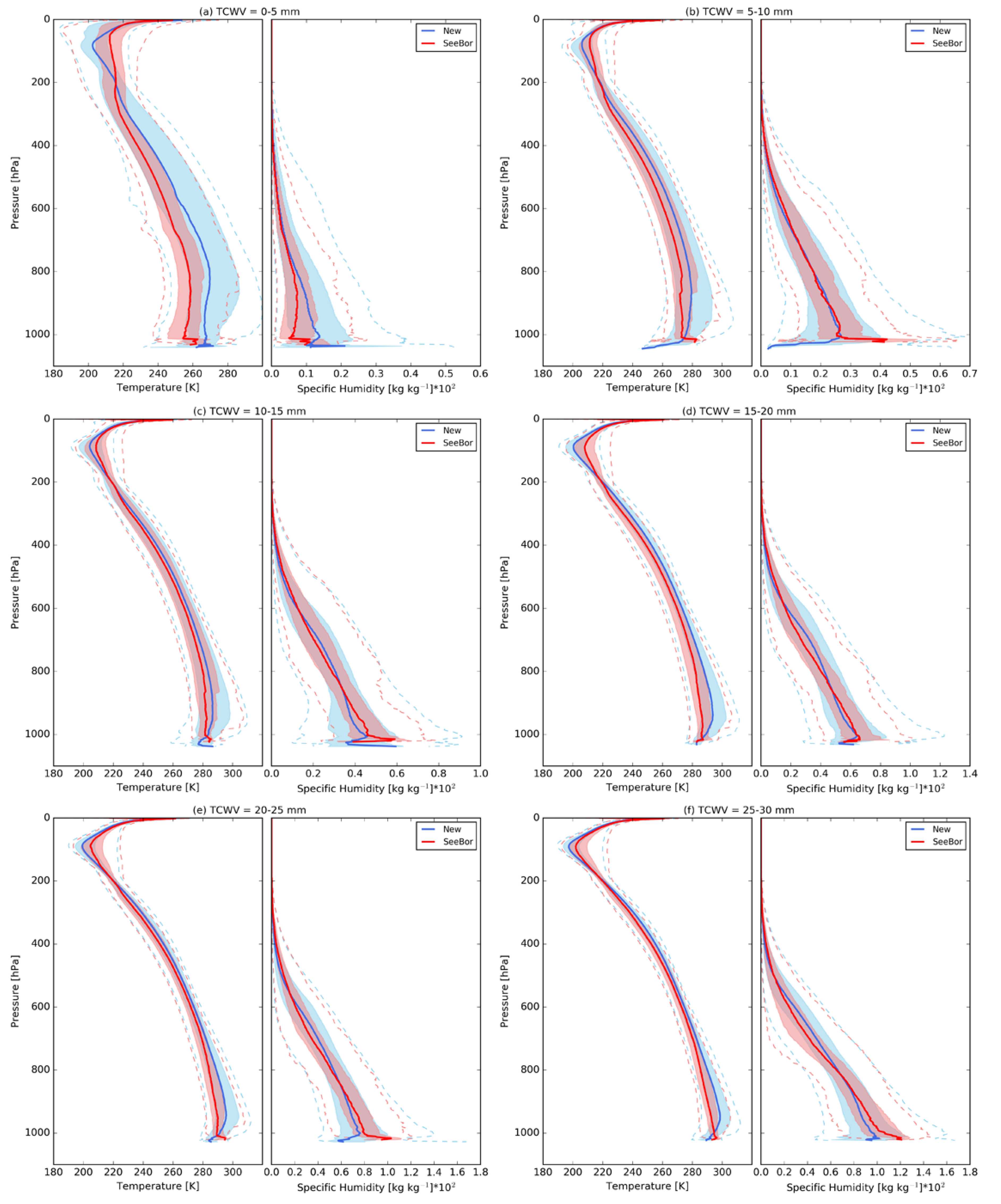
The vertical distribution of the selected temperature and water vapor profiles was analyzed by computing the 5th, 25th, 50th, 75th, and 95th percentiles of the two variables at each pressure level, for each TCWV class. Percentiles are used here instead of the mean and standard deviation since we found that distributions are mostly not symmetrical around the mean, and therefore the standard deviation may misrepresent the actual range of values.
Figure 4 shows these vertical distributions for each TCWV class. For reference, the respective distributions obtained from the SeeBor database are also shown. To obtain a consistent vertical grid, the profiles of both datasets are first interpolated to pressure levels. The two databases show distributions with significant differences, particularly in the lower troposphere, with the new database presenting a much wider range of values. Three main factors contribute to such differences: (1) the improved vertical resolution of ERA5 profiles compared to the data used in the Seebor database; (2) the wider range of conditions provided by ERA, which stems from a more realistic representation of atmospheric profiles (partially associated with the previous point) and surface variables when compared to Seeboor; (3) the used selection criterion that yields a more uniform distribution of the profiles within the database. The larger median and inter-quartile range of the temperature profile (and to some extent of the water vapor profile as well) in the lower TCWV class is particularly conspicuous. The SeeBor database does not represent the full range of temperature conditions that can occur under dry atmospheres, and the higher temperatures are underrepresented. The new database also seems to include values more extreme than the SeeBor, especially for low TCWV.
3.4. Distribution of Surface Conditions
3.4.1. Surface Temperature
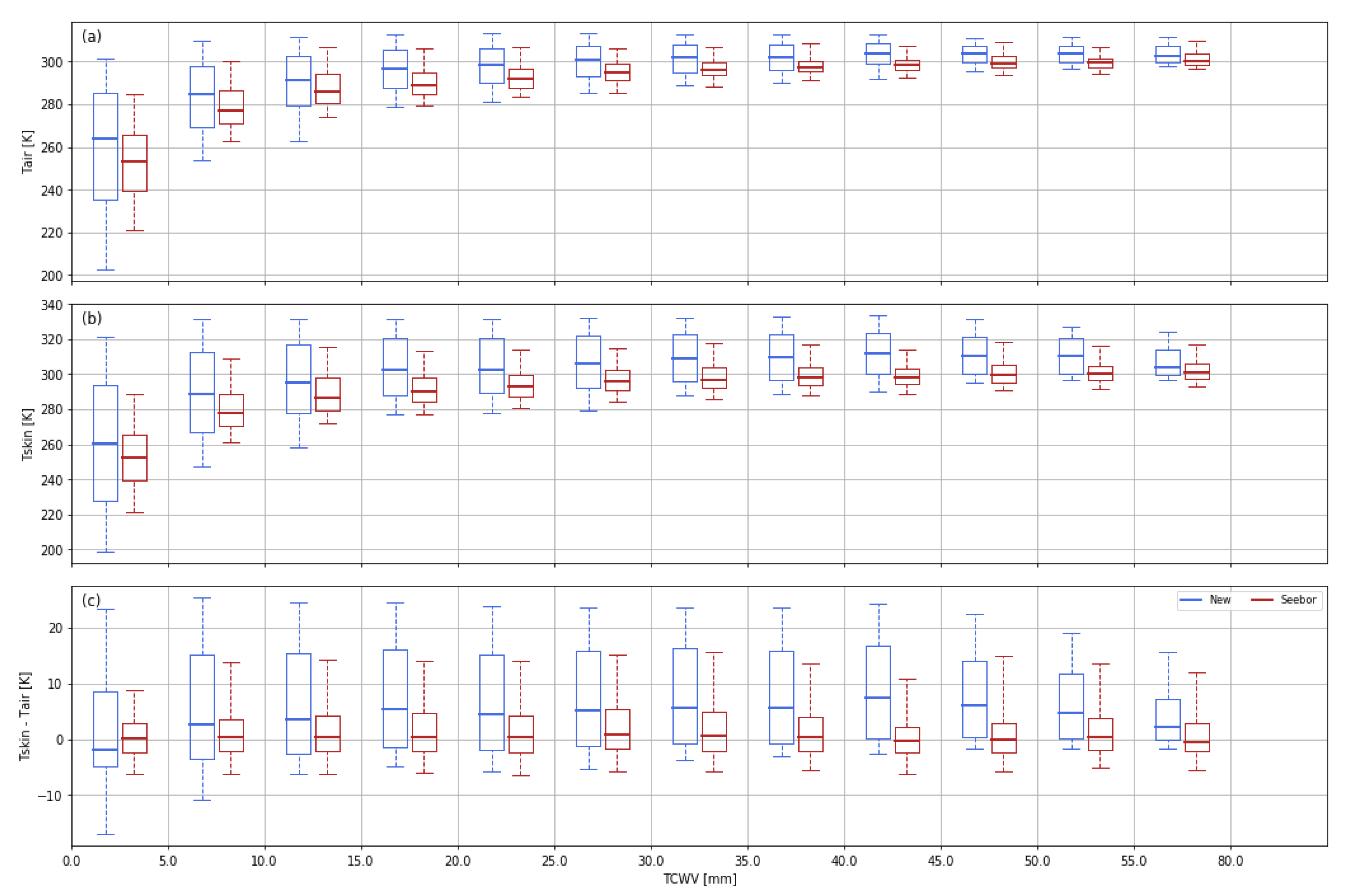
The surface variables obtained for each profile, namely surface air (first model level, corresponding to about 10 m above the surface) and skin temperatures (Tskin), as well as the difference between the two, were also analyzed. Figure 5 shows the obtained distributions for the selected profiles for each TCWV class. For reference, the respective distributions obtained from the SeeBor dataset are also shown. The proposed database shows a significant increase in the range of values of surface air and skin temperatures, especially for the lower TCWV. The range of skin temperature values is always significantly larger than in the case of SeeBor. In the SeeBor database, the skin temperature was prescribed as a function of surface air temperature and solar zenith and azimuth angles, based on station data from a single site. The use of only one site is likely not able to represent the full range of possible variability. The use of this empirical relationship between surface air and skin temperature is also noticeable when analyzing the distributions of the difference between the two variables (Figure 5, bottom panel), with the proposed database showing ranges of values around three times larger than that of the SeeBor. As such, the new database is likely to provide a more complete representation of the atmosphere-surface relationship.
Despite the great advances in surface modeling in the last decades, modeled Tskin still frequently presents large errors. In particular, several authors have pointed out a systematic underestimation of the Tskin in reanalysis datasets [2,8,10]. Tskin estimates should, therefore, be used with care in the context of algorithm/model calibration as the errors (in particular the systematic ones leading to an under-sampling of the Tskin actual distribution) will be propagated to the calibration and could significantly reduce the quality of the algorithm/model.
Satellite products of LST have been demonstrated to have good quality on average [56,60,61]. To reduce the propagation of satellite product errors to the calibration data, our strategy is to define an acceptable range of values of LST given the atmospheric conditions, taking as a baseline the estimates of Tskin.
For that purpose, LST estimates from the SEVIRI/MSG/MSG-IODC, ABI/GOES-R, ABI/HIMAWARI8, and AVHRR/EPS were collocated with estimates of surface variables from the ERA5 dataset. This wide range of sensors is used to ensure: (1) coverage of the full diurnal cycle for most of the globe, which is achieved through the constellation of geostationary satellites; (2) global coverage, namely by including a polar orbiter that provides data of the geostationary’ s coverage (mainly the poles). Figure 6 shows the distribution of the differences between LST and ERA5 Tskin using all satellite products.
To extend the range of Tskin values in the database, we take the 5th (95th) of the LST-Tskin difference to define the upper (lower) limit of the Tskin range in the calibration database. By leaving out LST values below/above the 5th/95th percentiles, we ensure that outliers, either related to errors in the LST products, such as cloud contamination, or events that will not be properly represented in ERA5, such as hotspots associated with wildfires or volcanic activity, are not included in the database. Since cloud contamination of the LST is more probable for high TCWV, for the last two classes of TCWV, the 10th percentile is used instead as the lower limit. This is noticeable in Figure 6, in the conspicuously low 5th percentile values of the 50–55 mm and 55–80 mm TCWV classes at a Tskin of 290–300 K (bottom panel, in grey and red). The range of Tskin in the new database is then increased by defining five equally spaced values between the two prescribed limits. As a result, to each profile, we attribute six Tskin values consisting of the original ERA5 value plus five new ones obtained from the satellite data.
This process is not intended to provide the actual values of Tskin corresponding to each profile but to provide a realistic range of Tskin for the given atmospheric conditions while increasing the representativeness of the database. This is likely to be more relevant for classes of low TCWV and low Tskin where we see a strong bias in ERA5 Tskin with respect to satellite LST (Figure 6).
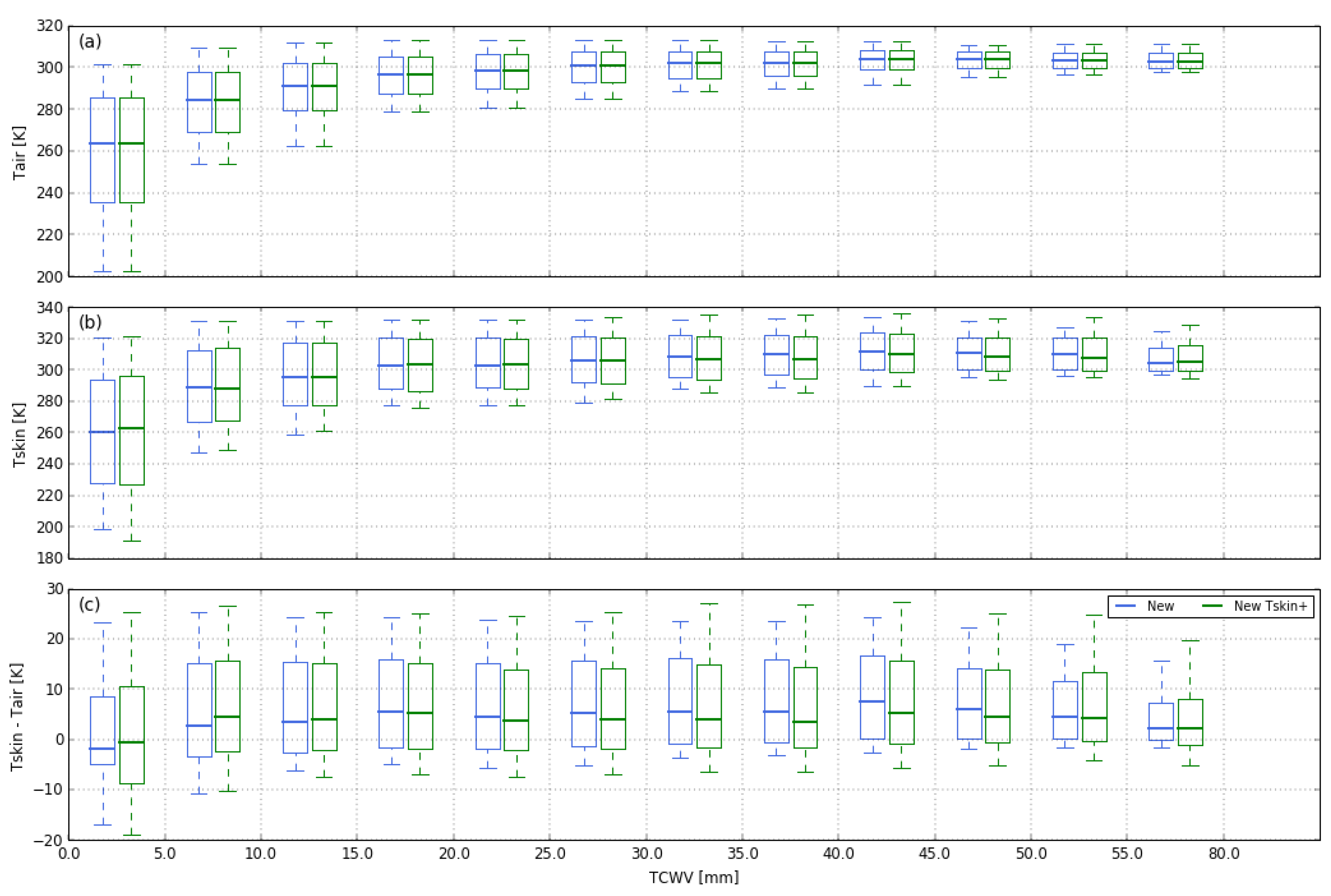
Figure 7 shows the new distribution of skin and surface air temperatures with the extended range of Tskin. This modification leads to a slight increase in the Tskin range, particularly increasing the range of the lower Tskin values for low TCWV and the range of the higher Tskin values for high TCWV. As expected, by attributing different Tskin values to each profile, the values of Tskin-Tair also show slight changes in the distribution.
3.4.2. Surface Emissivity
Land surface emissivity is one of the variables related to LST retrieval with the highest uncertainty [7]. To reduce the impact of those uncertainties on the calibration database, we opt to use a similar strategy to the one proposed for Tskin, where a range of possible emissivity values is defined that is consistent with the surface conditions.
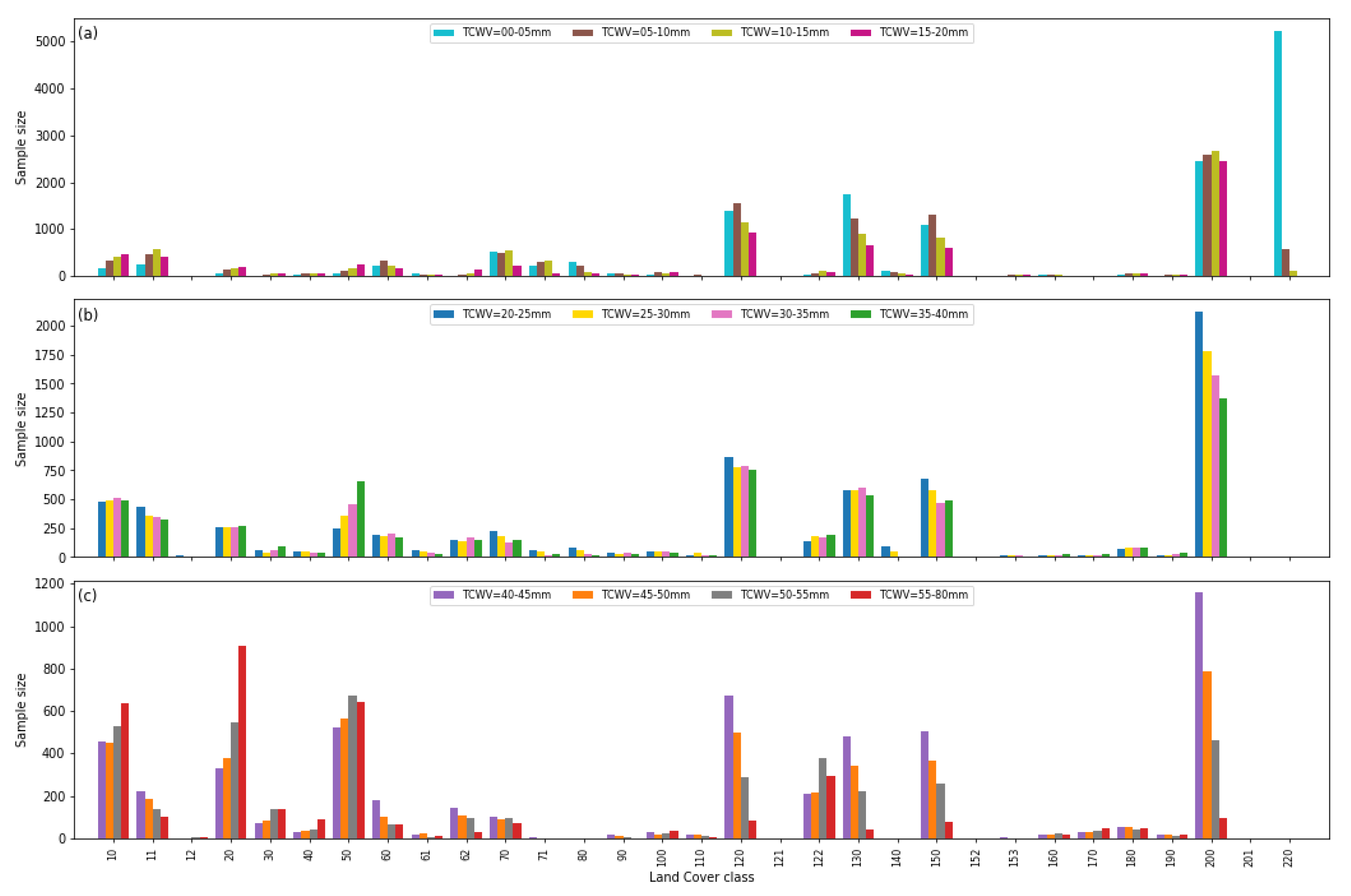
To create this range, we start by attributing a landcover type to each profile. Figure 8 shows the distribution of landcover types for each TCWV class. The database includes a wide range of landcover types: the lower TCWV classes encompass mostly snow (220), desert (200), and sparser vegetation types (120, 130, 150); as TCWV increases, there is a predominance of vegetated landcovers such as croplands (10–20), forest (50–90) and sparse/low vegetation (120–150).
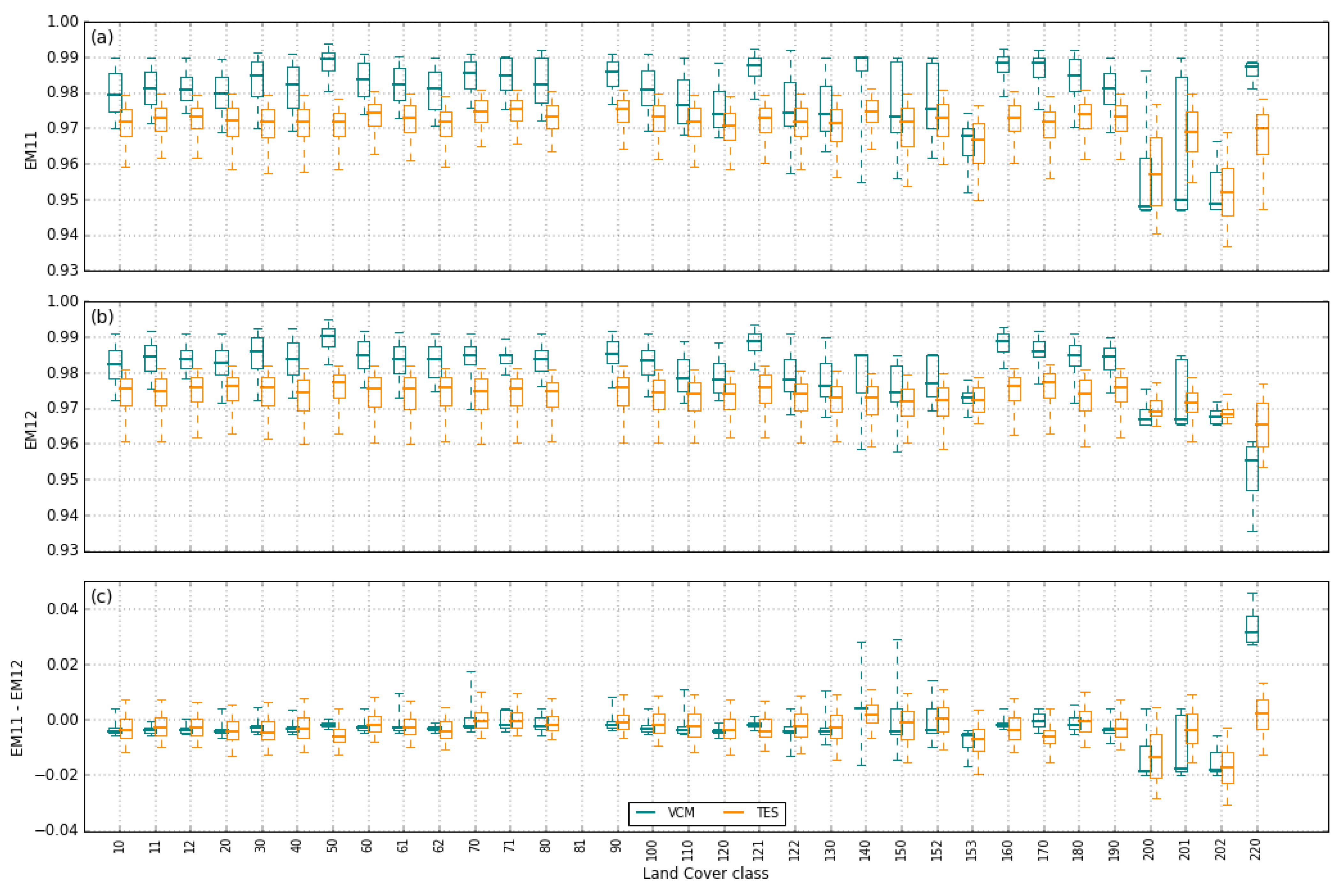
A range of emissivity values is attributed to each landcover type by using the satellite-based emissivity estimates. The distribution of the emissivity values is analyzed by landcover class (Figure 9). Although the different products will have slight differences due to changes in the spectral response function, we assume that variability due to the type of surface is much larger than that related to the sensor configuration. The TES method used in the MYD21 product is generally more accurate for bare areas, while the VCM is more accurate over vegetated areas where spectral contrasts are reduced [62,63]. As such, for vegetated classes, we use the VCM method as the upper limit (95th percentile) of the emissivity range and the TES as the lower limit (5th percentile) by assuming that when the vegetation cover is very low, the TES can better retrieve the soil emissivity. For desert classes, the TES range is used, while for snow/ice, only the VCM range is used since this yields values closer to those typically seen in spectral libraries. In the case of the emissivity difference between channels, we take the range of values given by TES as it should provide better estimates for higher spectral contrasts and therefore generally shows higher variability, with the exception of the snow/ice class where the VCM is used. Emissivity values are prescribed in the calibration in 2 steps:
- Five emissivity values are set for the ~11 µm channel taking equally spaced values in the emissivity range selected based on landcover (as described above);
- For each emissivity value prescribed in 1), five values of emissivity difference are set, taking equally spaced values in the selected emissivity difference range, which are used to compute the emissivities of the ~12 µm channel. Values above 0.99 are discarded.
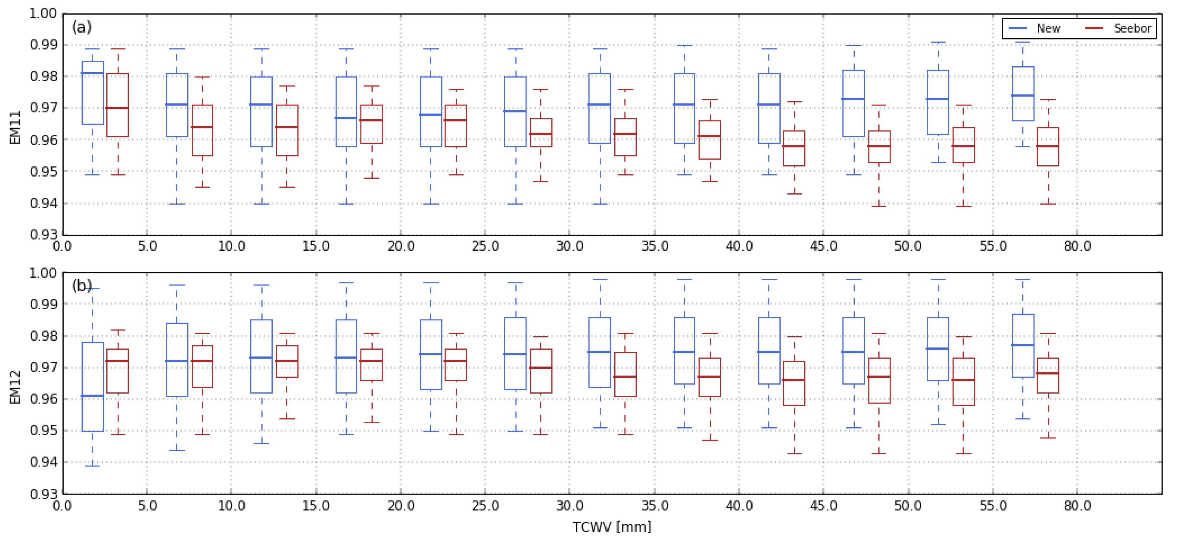
This method generates 25 pairs of emissivity at ~11 µm and ~12 µm for each profile. Figure 10 shows the resulting distribution of emissivity values in the new calibration database, together with the respective distributions from the SeeBor dataset. The proposed database provides a much wider range of emissivity values than the SeeBor. Emissivity values of the proposed database tend to be higher for higher TCWV, which is consistent with a higher vegetation density generally observed over wet regions.
3.5. Brightness Temperature Distribution
Lastly, we analyze the impact of the used sampling methodology on the corresponding top-of-atmosphere (TOA) brightness temperatures (BT). For that purpose, TOA BTs were computed for each database using the MODTRAN6 radiative transfer model. The MODTRAN6 output was then convolved with the response functions of SEVIRI/MSG3 channels 9 (centered at 10.8 µm) and 10 (centered at 12.0 µm). These two channels were selected since they are located in the TIR atmospheric window, being the most widely used channels in LST retrieval algorithms [7]. The outcome of the analysis performed for the corresponding simulated BTs largely applies to similar bands from other instruments.
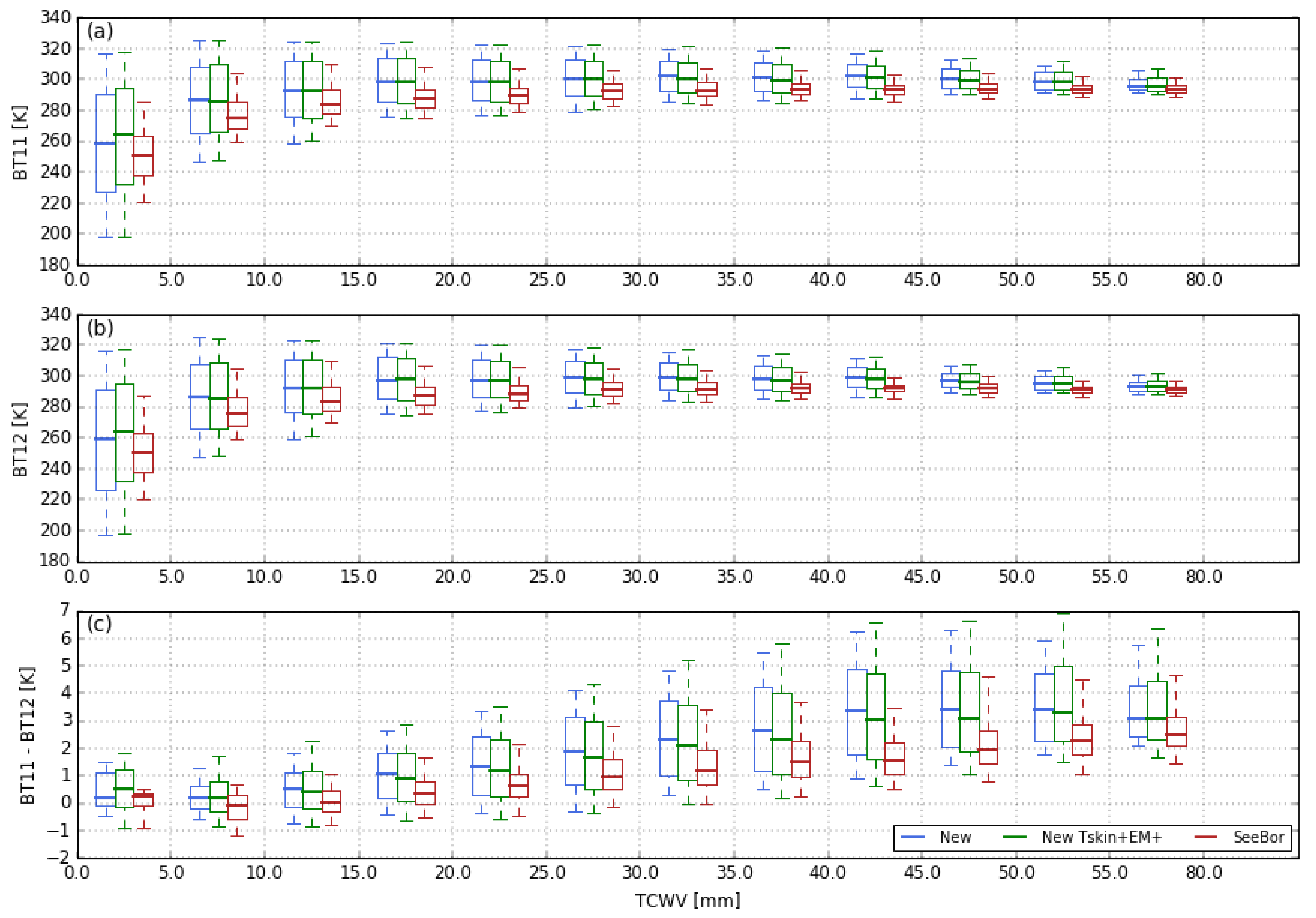
Figure 11 shows the distribution of BT for the two channels and the difference between them. To further understand the impact of increasing the variability of surface conditions for each profile, here we show the distribution for the proposed database when the Tskin from ERA5 is used together with a median value of emissivity for each landcover and when the range of Tskin and emissivities is extended based on the satellite data. For reference, the respective distribution for the SeeBor database is also shown. As expected from the previous analyses, the range of BT values significantly increases compared to the SeeBor database, and the medians of the BTs are always higher. This is a direct consequence of the higher median and range of the Tskin in the proposed database (Figure 5). There is also a significant increase in the range of BT difference, which is of high importance for the quality of the atmospheric correction in algorithms using the split-window channels [7,28].
The increased range of atmospheric profiles already introduces a significant increase in the range of Tskin values (Figure 5), which contributes to the wider range of BTs seen in Figure 11. The extension of the surface conditions shows only a marginal increase in the range of BTs. The extension of the surface conditions seems to be relevant, nonetheless, to increase the range of the BT differences. Likely, the increased variability in emissivity values helps to define better the contributions of the emissivity and the atmosphere to the BT difference.
4. Impact on Algorithm Calibration
Here we provide a comprehensive dataset that can be used for training algorithms of LST retrieval. It is well understood in modern statistics that, besides the model selection and a priori information, the resampling method is essential for robust model parameter estimation [64]. These resample methods involve splitting the full database into training and testing sets and they help prevent overfitting of the reference data. Although resampling methods can sometimes be demanding (they usually require fitting the model multiple times), with today’s computing capabilities, we believe they could be a great added value for designing an accurate and robust retrieval procedure.
Two of the most commonly used categories of resampling methods are cross-validation and bootstrap [64]. Xu and Goodacre [65] show that different variations of these methods show consistent, correct classification rates, particularly for large sample sizes (around 1000). The cross-validation methods are useful to avoid over-fitting the training data. A popular cross-validation method is a k-fold cross-validation, where the samples are subdivided into k parts (or folds) of approximately equal size, with k-1 folds serving as the training dataset and the remaining single fold being held out as the validation one [64]. The process is repeated k times so that ultimately all folds have been used for validation. The performance of the model is then given by the average of all the k validation exercises, and the optimal model parameters are those with the best performance. Typical values of k are 5 and 10, which means that this method is particularly appropriate for computationally expensive models.
Bootstrap techniques also provide an estimate of the uncertainty of the model [66], which is particularly useful for learning methods where a measure of variability is difficult to obtain (e.g., machine learning methods). The bootstrap also allows identifying statistically non-significant coefficients in a model. With a bootstrap method, a subset of samples (with the same size as the original dataset) is randomly selected with replacement and used as the training set. The samples that were not selected are used for validation. The process is repeated a high number of times (e.g., 100 or 1000 depending on the size of the original dataset) and the final performance of the model is taken to be the average from all validation exercises.
A combination of cross-validation and bootstrap, such as the Monte-Carlo Cross-Validation (MCCV) [67], could also be particularly appropriate to incorporate the best value of each method. Similar to the cross-validation, with the MCCV, a subset of samples is randomly selected (typically 25–30% of the original sample size) but without replacement to train the model leaving the remaining samples for validation. The process is repeated a high number of times, like with the bootstrap. The final estimated performance of the model is also the average of the predictive performance of each of the repeats of the cross-validation.
To further assess the impact of the newly developed database on algorithm calibration exercises, we here test the calibration of the Generalized Split-Window (GSW) algorithm used within the framework of the LSA-SAF [26,28]. In this formulation, the LST is estimated as a function of TOA BT of channels 9 (10.8 µm) and 10 (12.0 µm):
where is the average emissivity of the two channels and their difference. Aj, Bj, and C (j = 1,2,3) are the GSW coefficients obtained by fitting equation 4 to the calibration database. These coefficients are usually adjusted for classes of TCWV and satellite view zenith angle (VZA). For this exercise, the TCWV classes are the same as previously defined for the creation of the new database, i.e., varying from 0 to 60 mm in steps of 5 mm. The VZA classes are defined as varying between 0° and 70° in steps of 5°.
TOA BT values are also obtained using the MODTRAN6 radiative transfer model. The performance of the algorithm is assessed using the MCCV approach: for each TCWV and VZA class, 1/3 of the samples are randomly selected for training, and the remaining are used for validation; the calibration process is repeated 50 times, with a new set of coefficients and respective root mean squared error (RMSE) being estimated each time. This exercise is performed using the new and the SeeBor databases. We consider that the new database provides a better reference for validation given the improved representation of the troposphere and the much wider range of atmospheric and surface conditions included. Nevertheless, for reference, each model is also compared against the validation subset of the SeeBor database.
Figure 12 shows the distribution of RMSE as obtained when training the GSW algorithm with the new database (blue tones) and with the SeeBor database (red tones) and validated against the new database (upper panel) and the SeeBor database (lower panel). To simplify the visualization, the figure only shows the values obtained for the VZA classes of 0° to 5° and 65° to 70°, which generally correspond to the best and poorer performances of the GSW, respectively. When validated against the new database (Figure 12a), the models trained with the SeeBor database present higher RMSE values than those obtained when training the model with the new database. This difference in performance is particularly evident for higher VZAs, when the atmospheric correction is more complex. Also noteworthy is the much higher variability of the RMSE values in the case of the SeeBor-trained models. This behavior suggests that calibration exercises with this database are much more sensitive to the sub-setting of training and validation datasets. On the other hand, the new database allows for a very robust fit, with very little variability between iterations. This is a result of the much higher number of samples combined with the uniform distribution of the profiles. The effect of the database on the robustness of fit is also visible when analyzing the actual GSW coefficients (Figure S1 of the supplementary material), which show a much higher variability when trained with the SeeBor database.
When validating the models with the SeeBor database (Figure 12b), the performance of the GSW trained using the two databases is similar. However, the RMSE values are significantly lower than those obtained when validating with the new database, particularly in the case of SeeBor-trained models. This is to be expected, given the much more limited variability of atmospheric and surface conditions found in the SeeBor. The performance of the GSW models trained with the new database does not change significantly when the validation dataset is changed (i.e., when we use data from the new or from the SeeBor database), which also demonstrates the robustness of this dataset.
5. Discussion
Here we present a database of atmospheric profiles and surface conditions useful for the calibration of LST retrieval algorithms for satellite TIR observations. The database was built from the recent ERA5 reanalysis, taking full advantage of the advanced numerical weather predication and assimilation systems combined with a vast array of historical observations [54]. The use of reanalysis data has the advantage of not only providing high temporal and spatial coverage with good vertical resolution (137 levels) but also offering multiple atmospheric and surface variables that are consistent with each other.
The ERA5 profiles of temperature and specific humidity are resampled using the methodology of Chevallier et al. [38] for the TIGR-like database, where profiles are selected based on a dissimilarity criterion. This allows obtaining a more uniform distribution of atmospheric conditions, i.e., the database, and consequently any model calibrated with this database, will be less “biased” towards the most common conditions. We believe that resampling is of high importance in developing robust retrieval algorithms that can perform under all conditions. Furthermore, the TIGR-like datasets, and later the SeeBor database, were built on older versions of the ECMWF reanalysis. The most recent ERA5 represents a significant improvement from those older versions, especially in the lower layers of the atmosphere, which translates into a significant improvement in the simulation of satellite observations performed in wavelengths more sensitive to the surface.
Data from the ERA5 are further complemented with information from satellite-estimated surface temperature and emissivity. LST products from the SEVIRI/MSG/MSG-IODC, AVHRR/Metop, ABI/GOES-R, and AHI/Himawari are used to increase the range of possible skin temperature values for each profile, this way further increasing the representativeness of the database. This reduces the impact of possible biases in the ERA5 dataset on algorithm calibration. For instance, Johannsen et al. [8] identified a cold bias of ERA5 skin temperature in savanna-like landscapes. The analysis performed in this study shows a persistent overestimation of the skin temperature for very cold surfaces (snow/ice). Emissivity data from the same sensors, together with TES-retrieved values from MODIS/Aqua, were also used to define acceptable values of emissivity for each landcover type. It should be noted that these satellite data are not directly used in the dataset to avoid propagating product errors onto the training data. Instead, they are used to describe the variability of surface conditions realistically. Our analysis suggests that the increase in the skin temperature range may have a small impact on the overall distribution of brightness temperatures, but it is essential to circumvent some of the limitations identified in the ERA5 data. On the other hand, the wider range of emissivity values is relevant when considering the between channel difference in brightness temperature.
Compared to the widely used SeeBor [27], the proposed database shows a significantly wider range of conditions, both in terms of temperature and specific humidity profiles and in terms of surface and near-surface conditions. This is to be expected given the significant advancement of the ERA5 with respect to the ERA-40, which was used in SeeBor. This larger variability translates into a much wider range of brightness temperatures.
We also briefly discuss some re-sampling methods that can be followed in algorithm calibration exercises with this new dataset. Monte Carlo or bootstrap-like methods have the advantage of providing a confidence interval or the variance of the model parameters, while cross-validation is desirable to avoid over-fitting the training data. Naturally, any resampling method can be applied to the dataset for training any model, and the presented ones are a small set of a wide array of available methods. The pros and cons of each method are widely discussed in the literature (e.g., [64,65,68]). We then use a Monte-Carlo Cross-Validation to evaluate how the performance of a Generalized Split-Window algorithm calibrated with the new database compares to the one calibrated with the SeeBor database. Results show that the new database enables more robust fits, with no significant changes in performance between iterations. The SeeBor database, on the other hand, yields highly variable coefficients and RMSEs, suggesting that calibration exercises with this database will be highly sensitive to the actually selected training subset.
This work was carried out within the framework of the LSA-SAF project to create a training database for the development of LST retrieval algorithms for the next generation of satellites from the European Organization for the Exploitation of Meteorological Satellites (EUMETSAT), the Metop Second Generation, and the Meteosat Third Generation. As such, the dataset includes only data over land and for clear-sky conditions. Nevertheless, the dataset may be easily extended to include water surfaces and cloudy conditions. Although the database described here targets, in particular, the development of LST algorithms, it can be used for the development of other land surface products relying on optical/thermal infrared imagery and that will benefit from a wide and realistic sampling of surface and atmospheric conditions.
Supplementary Materials
The following supporting information can be downloaded at: https://0-www-mdpi-com.brum.beds.ac.uk/article/10.3390/rs14102329/s1, Figure S1: Distribution of model coefficients as obtained from 50 GSW model fits using the new database (blue colors) and the SeeBor database (red colors). Distributions are shown for each TCWV class (x-axis) and for VZA classes of 0° to 5° (darker colors) and of 65° to 70° (lighter colors). The bold line represents the median, the box represents the 25th to 75th percentiles, and the whiskers represent the 5th and 95th percentiles.
Author Contributions
Conceptualization, S.L.E. and I.F.T.; Data curation, S.L.E.; Formal analysis, S.L.E.; Funding acquisition, I.F.T.; Investigation, S.L.E.; Methodology, S.L.E. and I.F.T.; Project administration, I.F.T.; Resources, I.F.T.; Software, S.L.E.; Supervision, I.F.T.; Validation, S.L.E.; Visualization, S.L.E.; Writing—original draft, S.L.E.; Writing—review & editing, I.F.T. All authors have read and agreed to the published version of the manuscript.
Funding
This work was performed within the framework of the LSA SAF (http://lsa-saf-eumetsat.int) project, funded by EUMETSAT.
Institutional Review Board Statement
Not applicable.
Informed Consent Statement
Not applicable.
Data Availability Statement
This dataset is freely available at: https://0-doi-org.brum.beds.ac.uk/10.5281/zenodo.5779543 [69].
Acknowledgments
A special thank you to Carlos da Camara for his input on the dissimilarity criteria.
Conflicts of Interest
The authors declare no conflict of interest.
References
- Balsamo, G.; Agusti-Panareda, A.; Albergel, C.; Arduini, G.; Beljaars, A.; Bidlot, J.; Blyth, E.; Bousserez, N.; Boussetta, S.; Brown, A.; et al. Satellite and In Situ Observations for Advancing Global Earth Surface Modelling: A Review. Remote Sens. 2018, 10, 2038. [Google Scholar] [CrossRef] [Green Version]
- Trigo, I.F.; Boussetta, S.; Viterbo, P.; Balsamo, G.; Beljaars, A.; Sandu, I. Comparison of model land skin temperature with remotely sensed estimates and assessment of surface-atmosphere coupling. J. Geophys. Res. Atmos. 2015, 120, 12096–12111. [Google Scholar] [CrossRef] [Green Version]
- Mildrexler, D.J.; Zhao, M.; Running, S.W. Satellite Finds Highest Land Skin Temperatures on Earth. Bull. Am. Meteorol. Soc. 2011, 92, 855–860. [Google Scholar] [CrossRef] [Green Version]
- Miralles, D.G.; van den Berg, M.J.; Teuling, A.J.; de Jeu, R.A.M. Soil moisture-temperature coupling: A multiscale observational analysis. Geophys. Res. Lett. 2012, 39. [Google Scholar] [CrossRef] [Green Version]
- Su, Z. The Surface Energy Balance System (SEBS) for estimation of turbulent heat fluxes. Hydrol. Earth Syst. Sci. 2002, 6, 85–100. [Google Scholar] [CrossRef]
- Bojinski, S.; Verstraete, M.; Peterson, T.C.; Richter, C.; Simmons, A.; Zemp, M. The Concept of Essential Climate Variables in Support of Climate Research, Applications, and Policy. Bull. Am. Meteorol. Soc. 2014, 95, 1431–1443. [Google Scholar] [CrossRef]
- Li, Z.-L.; Tang, B.-H.; Wu, H.; Ren, H.; Yan, G.; Wan, Z.; Trigo, I.F.; Sobrino, J. A Satellite-derived land surface temperature: Current status and perspectives. Remote Sens. Environ. 2013, 131, 14–37. [Google Scholar] [CrossRef] [Green Version]
- Johannsen, F.; Ermida, S.; Martins, J.P.A.; Trigo, I.F.; Nogueira, M.; Dutra, E. Cold Bias of ERA5 Summertime Daily Maximum Land Surface Temperature over Iberian Peninsula. Remote Sens. 2019, 11, 2570. [Google Scholar] [CrossRef] [Green Version]
- Orth, R.; Dutra, E.; Trigo, I.F.; Balsamo, G. Advancing land surface model development with satellite-based Earth observations. Hydrol. Earth Syst. Sci. 2017, 21, 2483–2495. [Google Scholar] [CrossRef] [Green Version]
- Nogueira, M.; Boussetta, S.; Balsamo, G.; Albergel, C.; Trigo, I.F.; Johannsen, F.; Miralles, D.G.; Dutra, E. Upgrading Land-Cover and Vegetation Seasonality in the ECMWF Coupled System: Verification With FLUXNET Sites, METEOSAT Satellite Land Surface Temperatures, and ERA5 Atmospheric Reanalysis. J. Geophys. Res. Atmos. 2021, 126, e2020JD034163. [Google Scholar] [CrossRef]
- Kogan, F.N.; Kogan, F.N. Operational Space Technology for Global Vegetation Assessment. Bull. Am. Meteorol. Soc. 2001, 82, 1949–1964. [Google Scholar] [CrossRef]
- Kumar, D.; Shekhar, S. Statistical analysis of land surface temperature–vegetation indexes relationship through thermal remote sensing. Ecotoxicol. Environ. Saf. 2015, 121, 39–44. [Google Scholar] [CrossRef] [PubMed]
- Bento, V.A.; Gouveia, C.M.; DaCamara, C.C.; Trigo, I.F. A climatological assessment of drought impact on vegetation health index. Agric. For. Meteorol. 2018, 259, 286–295. [Google Scholar] [CrossRef]
- Albright, T.P.; Pidgeon, A.M.; Rittenhouse, C.D.; Clayton, M.K.; Flather, C.H.; Culbert, P.D.; Radeloff, V.C. Heat waves measured with MODIS land surface temperature data predict changes in avian community structure. Remote Sens. Environ. 2011, 115, 245–254. [Google Scholar] [CrossRef] [Green Version]
- Jiménez, C.; Michel, D.; Hirschi, M.; Ermida, S.; Prigent, C. Applying multiple land surface temperature products to derive heat fluxes over a grassland site. Remote Sens. Appl. Soc. Environ. 2017, 6. [Google Scholar] [CrossRef] [Green Version]
- Mokhtari, A.; Noory, H.; Pourshakouri, F.; Haghighatmehr, P.; Afrasiabian, Y.; Razavi, M.; Fereydooni, F.; Sadeghi Naeni, A. Calculating potential evapotranspiration and single crop coefficient based on energy balance equation using Landsat 8 and Sentinel-2. ISPRS J. Photogramm. Remote Sens. 2019, 154, 231–245. [Google Scholar] [CrossRef]
- Andersson, E.; Bauer, P.; Beljaars, A.; Chevallier, F.; Hólm, E.; Janisková, M.; Kallberg, P.; Kelly, G.; Lopez, P.; McNally, A.; et al. Assimilation and modeling of the atmospheric hydrological cycle in the ECMWF forecasting system. Bull. Am. Meteorol. Soc. 2005. [Google Scholar] [CrossRef] [Green Version]
- Bechtel, B.; Daneke, C. Classification of Local Climate Zones Based on Multiple Earth Observation Data. IEEE J. Sel. Top. Appl. Earth Obs. Remote Sens. 2012, 5, 1191–1202. [Google Scholar] [CrossRef]
- Fu, P.; Weng, Q. A time series analysis of urbanization induced land use and land cover change and its impact on land surface temperature with Landsat imagery. Remote Sens. Environ. 2016, 175, 205–214. [Google Scholar] [CrossRef]
- Rogan, J.; Ziemer, M.; Martin, D.; Ratick, S.; Cuba, N.; DeLauer, V. The impact of tree cover loss on land surface temperature: A case study of central Massachusetts using Landsat Thematic Mapper thermal data. Appl. Geogr. 2013, 45, 49–57. [Google Scholar] [CrossRef]
- Maimaitiyiming, M.; Ghulam, A.; Tiyip, T.; Pla, F.; Latorre-Carmona, P.; Halik, Ü.; Sawut, M.; Caetano, M. Effects of green space spatial pattern on land surface temperature: Implications for sustainable urban planning and climate change adaptation. ISPRS J. Photogramm. Remote Sens. 2014, 89, 59–66. [Google Scholar] [CrossRef] [Green Version]
- Peng, J.; Jia, J.; Liu, Y.; Li, H.; Wu, J. Seasonal contrast of the dominant factors for spatial distribution of land surface temperature in urban areas. Remote Sens. Environ. 2018, 215, 255–267. [Google Scholar] [CrossRef]
- Sobrino, J.A.; Julien, Y.; García-Monteiro, S. Surface Temperature of the Planet Earth from Satellite Data. Remote Sens. 2020, 12, 218. [Google Scholar] [CrossRef] [Green Version]
- Zhou, C.; Wang, K. Land surface temperature over global deserts: Means, variability, and trends. J. Geophys. Res. Atmos. 2016, 121, 357. [Google Scholar] [CrossRef]
- Bechtel, B. A New Global Climatology of Annual Land Surface Temperature. Remote Sens. 2015, 7, 2850–2870. [Google Scholar] [CrossRef] [Green Version]
- Trigo, I.F.; Monteiro, I.T.; Olesen, F.; Kabsch, E. An assessment of remotely sensed land surface temperature. J. Geophys. Res. 2008, 113, 1–12. [Google Scholar] [CrossRef]
- Borbas, E.E.; Seemann, S.W.; Huang, H.L.; Li, J.; Menzel, W.P. Global profile training database for satellite regression retrievals with estimates of skin temperature and emissivity. In Proceedings of the International TOVS Study Conference-XIV, Beijing, China, 25–31 May 2005. [Google Scholar]
- Wan, Z.; Dozier, J. A generalized split-window algorithm for retrieving land-surface temperature from space. Geosci. Remote Sens. IEEE Trans. 1996, 34, 892–905. [Google Scholar]
- Malakar, N.K.; Hulley, G.C. A water vapor scaling model for improved land surface temperature and emissivity separation of MODIS thermal infrared data. Remote Sens. Environ. 2016, 182, 252–264. [Google Scholar] [CrossRef]
- Ghent, D.J.; Corlett, G.K.; Göttsche, F.-M.; Remedios, J.J. Global Land Surface Temperature From the Along-Track Scanning Radiometers. J. Geophys. Res. Atmos. 2017, 122, 193. [Google Scholar] [CrossRef] [Green Version]
- Martins, J.; Trigo, I.; Bento, V.; da Camara, C. A Physically Constrained Calibration Database for Land Surface Temperature Using Infrared Retrieval Algorithms. Remote Sens. 2016, 8, 808. [Google Scholar] [CrossRef] [Green Version]
- Achard, V. Trois problèmes clés de l’analyse 3D de la structure thermodynamique de l’atmosphère par satellite: Mesure du contenu en ozone; classification des masses d’air; modélisation hyper rapide du transfert radiatif. Ph.D. Thesis, University of Paris, Paris, France, 1991. [Google Scholar]
- Chedin, A.; Scott, N.A.; Wahiche, C.; Moulinier, P.; Chedin, A.; Scott, N.A.; Wahiche, C.; Moulinier, P. The Improved Initialization Inversion Method: A High Resolution Physical Method for Temperature Retrievals from Satellites of the TIROS-N Series. J. Clim. Appl. Meteorol. 1985, 24, 128–143. [Google Scholar] [CrossRef] [Green Version]
- Chevallier, F.; Chéruy, F.; Scott, N.A.; Chédin, A. A Neural Network Approach for a Fast and Accurate Computation of a Longwave Radiative Budget. J. Appl. Meteorol. 1998, 37, 1385–1397. [Google Scholar] [CrossRef]
- Escobar-Munoz, J. Base de données pour la restitution de variables atmosphériques à l’échelle globale. Étude sur l’inversion par réseaux de neurones des données des sondeurs verticaux atmosphériques satellitaires présents et à venir. Ph.D. Thesis, University of Paris, Paris, France, 1993. [Google Scholar]
- Moulinier, P. Analyse Statistique d’un Vaste Echantillonnage de Situations Atmosphériques sur l’ensemble du Globe. Laboratoire de Météorologie Dynamique Internal note No. 123; École Polytechnique: Paris, France, 1983. [Google Scholar]
- Seemann, S.W.; Li, J.; Menzel, W.P.; Gumley, L.E. Operational Retrieval of Atmospheric Temperature, Moisture, and Ozone from MODIS Infrared Radiances. J. Appl. Meteorol. 2003, 42, 1072–1091. [Google Scholar] [CrossRef]
- Chevallier, F.; Chédin, A.; Cheruy, F.; Morcrette, J.-J. TIGR-like atmospheric-profile databases for accurate radiative-flux computation. Q. J. R. Meteorol. Soc. 2000, 126, 777–785. [Google Scholar] [CrossRef]
- Chevallier, F. Sampled database of 60-Level atmospheric profiles from the ECMWF analyses; NWPSAF Research Report No NWPSAF-EC-TR-004 (v1.0); Reading: Shinfield Park, UK, 2002. [Google Scholar]
- Saunders, R.; Hocking, J.; Turner, E.; Rayer, P.; Rundle, D.; Brunel, P.; Vidot, J.; Roquet, P.; Matricardi, M.; Geer, A.; et al. An update on the RTTOV fast radiative transfer model (currently at version 12). Geosci. Model Dev. 2018, 11, 2717–2737. [Google Scholar] [CrossRef] [Green Version]
- Chevallier, F.; Di Michele, S.; McNally, A. Diverse Profile Datasets from the ECMWF 91-Level Short-Range Forecasts; NWPSAF Research Report No NWPSAF-EC-TR-010 (v1.0); Reading: Shinfield Park, UK, 2006. [Google Scholar]
- Aires, F.; Prigent, C. Sampling techniques in high-dimensional spaces for the development of satellite remote sensing database. J. Geophys. Res. 2007, 112, D20301. [Google Scholar] [CrossRef] [Green Version]
- Mattar, C.; Durán-Alarcón, C.; Jiménez-Muñoz, J.C.; Santamaría-Artigas, A.; Olivera-Guerra, L.; Sobrino, J.A. Global Atmospheric Profiles from Reanalysis Information (GAPRI): A new database for earth surface temperature retrieval. Int. J. Remote Sens. 2015, 36, 5045–5060. [Google Scholar] [CrossRef]
- Choi, Y.-Y.; Suh, M.-S. Development of Himawari-8/Advanced Himawari Imager (AHI) Land Surface Temperature Retrieval Algorithm. Remote Sens. 2018, 10, 2013. [Google Scholar] [CrossRef] [Green Version]
- Duguay-Tetzlaff, A.; Bento, V.A.; Göttsche, F.M.; Stöckli, R.; Martins, J.P.A.; Trigo, I.; Olesen, F.; Bojanowski, J.S.; da Camara, C.; Kunz, H. Meteosat land surface temperature climate data record: Achievable accuracy and potential uncertainties. Remote Sens. 2015, 7, 13139–13156. [Google Scholar] [CrossRef] [Green Version]
- Freitas, S.C.; Trigo, I.F.; Macedo, J.; Barroso, C.; Silva, R.; Perdigão, R.; Freitas, S.C.; Trigo, I.F.; Macedo, J.; Barroso, C.; et al. Land surface temperature from multiple geostationary satellites. Int. J. Remote Sens. 2013, 1161. [Google Scholar] [CrossRef]
- Hulley, G.C.; Hook, S.J.; Abbott, E.; Malakar, N.; Islam, T.; Abrams, M. The ASTER Global Emissivity Dataset (ASTER GED): Mapping Earth’s emissivity at 100 meter spatial scale. Geophys. Res. Lett. 2015, 42. [Google Scholar] [CrossRef]
- Islam, T.; Hulley, G.C.; Malakar, N.K.; Radocinski, R.G.; Guillevic, P.C.; Hook, S.J. A Physics-Based Algorithm for the Simultaneous Retrieval of Land Surface Temperature and Emissivity From VIIRS Thermal Infrared Data. IEEE Trans. Geosci. Remote Sens. 2017, 55, 563–576. [Google Scholar] [CrossRef]
- Jiang, G.-M.; Zhou, W.; Liu, R. Development of Split-Window Algorithm for Land Surface Temperature Estimation From the VIRR/FY-3A Measurements. IEEE Geosci. Remote Sens. Lett. 2013, 10, 952–956. [Google Scholar] [CrossRef]
- Liu, X.; Tang, B.-H.; Yan, G.; Li, Z.-L.; Liang, S. Retrieval of Global Orbit Drift Corrected Land Surface Temperature from Long-term AVHRR Data. Remote Sens. 2019, 11, 2843. [Google Scholar] [CrossRef] [Green Version]
- Hulley, G.; Malakar, N.; Freepartner, R. Moderate Resolution Imaging Spectroradiometer (MODIS) Land Surface Temperature and Emissivity Product (MxD21) Algorithm Theoretical Basis Document Collection-6. Jet Propuls. Lab. Calif. Inst. Technol. 2016. [Google Scholar]
- Yang, J.; Zhou, J.; Göttsche, F.-M.; Long, Z.; Ma, J.; Luo, R. Investigation and validation of algorithms for estimating land surface temperature from Sentinel-3 SLSTR data. Int. J. Appl. Earth Obs. Geoinf. 2020, 91, 102136. [Google Scholar] [CrossRef]
- Zhou, J.; Liang, S.; Cheng, J.; Wang, Y.; Ma, J. The GLASS Land Surface Temperature Product. IEEE J. Sel. Top. Appl. Earth Obs. Remote Sens. 2019, 12, 493–507. [Google Scholar] [CrossRef]
- Hersbach, H.; Bell, B.; Berrisford, P.; Hirahara, S.; Horányi, A.; Muñoz-Sabater, J.; Nicolas, J.; Peubey, C.; Radu, R.; Schepers, D.; et al. The ERA5 global reanalysis. Q. J. R. Meteorol. Soc. 2020, 146, 1999–2049. [Google Scholar] [CrossRef]
- Chevallier, F. TIGR-Like Sampled Databases of Atmospheric Profiles from the ECMWF 50-Level Forecast Mode. NWPSAF Research Report No1; Reading: Shinfield Park, UK, 2000. [Google Scholar]
- Trigo, I.F.; Ermida, S.L.; Martins, J.P.A.; Gouveia, C.M.; Göttsche, F.-M.; Freitas, S.C. Validation and consistency assessment of land surface temperature from geostationary and polar orbit platforms: SEVIRI/MSG and AVHRR/Metop. ISPRS J. Photogramm. Remote Sens. 2021, 175, 282–297. [Google Scholar] [CrossRef]
- Peres, L.F.; DaCamara, C.C. Emissivity maps to retrieve land-surface temperature from MSG/SEVIRI. IEEE Trans. Geosci. Remote Sens. 2005, 43, 1834–1844. [Google Scholar] [CrossRef]
- Hulley, G.C.; Hook, S.J. MODIS/Aqua Land Surface Temperature/3-Band Emissivity Daily L3 Global 0.05Deg CMG V061 [Data set]. NASA EOSDIS Land Processes DAAC. 2021. Available online: https://www.ecmwf.int/node/8683 (accessed on 15 December 2021).
- CCI; ESA Land Cover. Product User Guide Version 2.0; UCL-Geomatics: London, UK, 2017. [Google Scholar]
- Ermida, S.L.; Trigo, I.F.; Dacamara, C.C.; Göttsche, F.M.; Olesen, F.S.; Hulley, G. Validation of remotely sensed surface temperature over an oak woodland landscape—The problem of viewing and illumination geometries. Remote Sens. Environ. 2014, 148, 16–27. [Google Scholar] [CrossRef]
- Göttsche, F.-M.; Olesen, F.-S.; Bork-Unkelbach, A. Validation of land surface temperature derived from MSG/SEVIRI with in situ measurements at Gobabeb, Namibia. Int. J. Remote Sens. 2013, 34, 3069–3083. [Google Scholar] [CrossRef]
- Jacob, F.; Lesaignoux, A.; Olioso, A.; Weiss, M.; Caillault, K.; Jacquemoud, S.; Nerry, F.; French, A.; Schmugge, T.; Briottet, X.; et al. Reassessment of the temperature-emissivity separation from multispectral thermal infrared data: Introducing the impact of vegetation canopy by simulating the cavity effect with the SAIL-Thermique model. Remote Sens. Environ. 2017, 198, 160–172. [Google Scholar] [CrossRef]
- Jiménez-Muñoz, J.C.; Sobrino, J.A.; Gillespie, A.; Sabol, D.; Gustafson, W.T. Improved land surface emissivities over agricultural areas using ASTER NDVI. Remote Sens. Environ. 2006, 103, 474–487. [Google Scholar] [CrossRef]
- James, G.; Witten, D.; Hastie, T.; Tibshirani, R. Resampling Methods. In An Introduction to Statistical Learning; Springer Texts in Statistics; Springer: New York, NY, USA, 2021; pp. 197–223. [Google Scholar]
- Xu, Y.; Goodacre, R. On Splitting Training and Validation Set: A Comparative Study of Cross-Validation, Bootstrap and Systematic Sampling for Estimating the Generalization Performance of Supervised Learning. J. Anal. Test. 2018, 2, 249–262. [Google Scholar] [CrossRef] [Green Version]
- Shao, J. Bootstrap Model Selection. J. Am. Stat. Assoc. 1996, 91, 655–665. [Google Scholar] [CrossRef]
- Shao, J. Linear Model Selection by Cross-validation. J. Am. Stat. Assoc. 1993, 88, 486–494. [Google Scholar] [CrossRef]
- Hastie, T.; Tibshirani, R.; Friedman, J. The Elements of Statistical Learning: Data Mining, Inference, and Prediction, 2nd ed; Springer Series in Statistics; Springer: New York, NY, USA, 2017; ISBN 978-0-387-84857-0. [Google Scholar]
- Ermida, S.L.; Trigo, I.F. Clear-Sky Profile Database for the Development of Land Surface Temperature Algorithms (v0.0.0) [Data Set]; Zenodo: Geneve, Switzerland, 2021. [Google Scholar] [CrossRef]
Figure 1.
Sample size of the original ERA5 (a) and the new calibration (b) databases for each TCWV (mm) and skin temperature (K) class.
Figure 1.
Sample size of the original ERA5 (a) and the new calibration (b) databases for each TCWV (mm) and skin temperature (K) class.

Figure 2.
Geographical distribution of the profiles selected for the atmospheric general database for each class of TCWV ((a) 0–5 mm; (b) 5–10 mm; (c) 10–15 mm; (d) 15–20 mm; (e) 20–25 mm; (f) 25–30 mm; (g) 30–35 mm; (h) 35–40 mm; (i) 40–45 mm; (j) 45–50 mm; (k) 50–55 mm; (l) 55–80 mm). Colors and respective colorbar indicate the corresponding class of Tskin (K).


Figure 3.
Histograms of local time (a) and of the month (b) of the selected data for the calibration database for each TCWV class.
Figure 3.
Histograms of local time (a) and of the month (b) of the selected data for the calibration database for each TCWV class.

Figure 4.
Distribution of the temperature (left) and specific humidity (right) profiles selected for the calibration database (blue) for each TCWV class ((a) 0–5 mm; (b) 5–10 mm; (c) 10–15 mm; (d) 15–20 mm; (e) 20–25 mm; (f) 25–30 mm; (g) 30–35 mm; (h) 35–40 mm; (i) 40–45 mm; (j) 45–50 mm; (k) 50–55 mm; (l) 55–80 mm). The solid lines represent the median, the shaded areas represent the 25th to 75th percentiles, and dashed lines represent the 5th and 95th percentiles. The distribution of the SeeBor profiles is also shown for reference (in red).


Figure 5.
Distribution of the (a) surface air temperature (Tair), (b) skin temperature (Tskin), and (c) the difference between skin and surface air temperatures for each TCWV class. The bold line represents the median, the box represents the 25th to 75th percentiles, and the whiskers represent the 5th and 95th percentiles. Values are shown for the new calibration database (blues) and the SeeBor database (red).

Figure 6.
Distribution of differences between satellite LST and ERA5 Tskin (K) for each TCWV class ((a) 0–5, 5–10, 10–15 and 15–20 mm; (b) 20–25, 25–30, 30–35 and 35–40 mm; (c) 40–45, 45–50, 50–55 and 55–80 mm). The bold line represents the median, the box represents the 25th to 75th percentiles, and the whiskers represent the 5th and 95th percentiles.

Figure 7.
As in Figure 5 but showing the proposed calibration database with extended Tskin range (Tskin+; green). . Distribution of the (a) surface air temperature (Tair), (b) skin temperature (Tskin), and (c) the difference between skin and surface air temperatures for each TCWV class
Figure 7.
As in Figure 5 but showing the proposed calibration database with extended Tskin range (Tskin+; green). . Distribution of the (a) surface air temperature (Tair), (b) skin temperature (Tskin), and (c) the difference between skin and surface air temperatures for each TCWV class

Figure 8.
Histograms of Landcover types (as described in Table 1) in the calibration database for each TCWV class ((a) 0–5, 5–10, 10–15 and 15–20 mm; (b) 20–25, 25–30, 30–35 and 35–40 mm; (c) 40–45, 45–50, 50–55 and 55–80 mm).
Figure 8.
Histograms of Landcover types (as described in Table 1) in the calibration database for each TCWV class ((a) 0–5, 5–10, 10–15 and 15–20 mm; (b) 20–25, 25–30, 30–35 and 35–40 mm; (c) 40–45, 45–50, 50–55 and 55–80 mm).

Figure 9.
Distribution of (a) ~11 µm (EM11), and (b) ~12 µm (EM12) emissivities, and (c) the between-channel emissivity difference, for the VCM (green) and TES methods (orange), for each landcover type (as described in Table 1). The bold line represents the median, the box represents the 25th to 75th percentiles, and the whiskers represent the 5th and 95th percentiles.

Figure 10.
Distribution of (a) ~11 µm (EM11), and (b) ~12 µm (EM12) emissivities for each TCWV class. The bold line represents the median, the box represents the 25th to 75th percentiles, and the whiskers represent the 5th and 95th percentiles. Values are shown for the new calibration database (blues) and the SeeBor database (red).

Figure 11.
Distribution of the TOA brightness temperature at (a) ~11 µm (BT11), and (b) ~12 µm (BT12), and (c) respective difference between the two, for each TCWV class. The bold line represents the median, the box represents the 25th to 75th percentiles, and the whiskers represent the 5th and 95th percentiles. Values are shown for the new calibration database with a single Tskin and emissivity value per profile (blues), for the new database with extended Tskin and emissivity values (Tskin+EM+; green) and the SeeBor database (red).

Figure 12.
Distribution of Root Mean Squared Errors (RMSE) as obtained from 50 GSW model fits using the new database (blue colors) and the SeeBor database (red colors) for training and using the new database (a) and the SeeBor database (b) for validation. Distributions are shown for each TCWV class (x-axis) and for VZA classes of 0° to 5° (darker colors) and 65° to 70° (lighter colors). The bold line represents the median, the box represents the 25th to 75th percentiles, and the whiskers represent the 5th and 95th percentiles.


Table 1.
CCI Landcover types’ description.
| ID | Description |
|---|---|
| 10 | Cropland, rainfed |
| 11 | Herbaceous cover |
| 12 | Tree or shrub cover |
| 20 | Cropland, irrigated or post-flooding |
| 30 | Mosaic cropland (>50%)/natural vegetation (tree, shrub, herbaceous cover) (<50%) |
| 40 | Mosaic natural vegetation (tree, shrub, herbaceous cover) (>50%) S/cropland (<50%) |
| 50 | Tree cover, broadleaved, evergreen, closed to open (>15%) |
| 60 | Tree cover, broadleaved, deciduous, closed to open (>15%) |
| 61 | Tree cover, broadleaved, deciduous, closed (>40%) |
| 62 | Tree cover, broadleaved, deciduous, open (15–40%) |
| 70 | Tree cover, needle-leaved, evergreen, closed to open (>15%) |
| 71 | Tree cover, needle-leaved, evergreen, closed (>40%) |
| 72 | Tree cover, needle-leaved, evergreen, open (15–40%) |
| 80 | Tree cover, needle-leaved, deciduous, closed to open (>15%) |
| 81 | Tree cover, needle-leaved, deciduous, closed (>40%) |
| 82 | Tree cover, needle-leaved, deciduous, open (15–40%) |
| 90 | Tree cover, mixed leaf type (broadleaved and needle-leaved) |
| 100 | Mosaic tree and shrub (>50%)/herbaceous cover (<50%) |
| 110 | Mosaic herbaceous cover (>50%)/tree and shrub (<50%) |
| 120 | Shrubland |
| 121 | Evergreen shrubland |
| 122 | Deciduous shrubland |
| 130 | Grassland |
| 140 | Lichens and mosses |
| 150 | Sparse vegetation (tree, shrub, herbaceous cover) (<15%) |
| 151 | Sparse tree (<15%) |
| 152 | Sparse shrub (<15%) |
| 153 | Sparse herbaceous cover (<15%) |
| 160 | Tree cover, flooded, fresh, or brackish water |
| 170 | Tree cover, flooded, saline water |
| 180 | Shrub or herbaceous cover, flooded, fresh/saline/brackish water |
| 190 | Urban areas |
| 200 | Bare areas |
| 201 | Consolidated bare areas |
Publisher’s Note: MDPI stays neutral with regard to jurisdictional claims in published maps and institutional affiliations. |
© 2022 by the authors. Licensee MDPI, Basel, Switzerland. This article is an open access article distributed under the terms and conditions of the Creative Commons Attribution (CC BY) license (https://creativecommons.org/licenses/by/4.0/).
Share and Cite
MDPI and ACS Style
Ermida, S.L.; Trigo, I.F. A Comprehensive Clear-Sky Database for the Development of Land Surface Temperature Algorithms. Remote Sens. 2022, 14, 2329. https://0-doi-org.brum.beds.ac.uk/10.3390/rs14102329
AMA Style
Ermida SL, Trigo IF. A Comprehensive Clear-Sky Database for the Development of Land Surface Temperature Algorithms. Remote Sensing. 2022; 14(10):2329. https://0-doi-org.brum.beds.ac.uk/10.3390/rs14102329
Chicago/Turabian StyleErmida, Sofia L., and Isabel F. Trigo. 2022. "A Comprehensive Clear-Sky Database for the Development of Land Surface Temperature Algorithms" Remote Sensing 14, no. 10: 2329. https://0-doi-org.brum.beds.ac.uk/10.3390/rs14102329
Note that from the first issue of 2016, this journal uses article numbers instead of page numbers. See further details here.