A Dataset of Overshooting Cloud Top from 12-Year CloudSat/CALIOP Joint Observations

Abstract

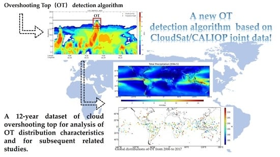
A strong convective storm is a disastrous weather system with a small spatio-temporal scale. It often occurs suddenly and can cause huge disasters. Thus, it is necessary to improve the forecast accuracy of strong convective storms. Overshooting cloud top (OT) is the product of strong updrafts in convective storms, which can penetrate the tropopause and enter the lower stratosphere. OT is closely related to severe weather and can influence water vapor transport and the material exchange between the troposphere and stratosphere. Therefore, the timely detection of OT can help improve the accuracy of forecasting. In this study, we develop a new objective OT detection algorithm based on geostationary satellite observations from 2006 to 2017. The accuracy of the new algorithm in identifying OT is verified by manually comparing it with the radar echo images and the cloud images of MODIS 250 m. Then, the OT is statistically analyzed in a long time series. It is found that OT events are mainly concentrated in equatorial and low latitude regions, with higher frequency in summer. There are obvious differences between OT events on land and sea. Additionally, this dataset also reveals the close connection between the seasonal shift of OT and the seasonal average precipitation distribution around the globe. This study provides a scientific basis for determining the geographical characteristics of OT frequency and explores the application of this OT objective detection algorithm in the operational forecast of strong convective weather. We hope this study can benefit OT monitoring in operational weather forecasting.

1. Introduction

Under strong vertical wind shear, strong convective storms often occur suddenly and develop rapidly, and can cause severe disasters, such as tornadoes, hail, thunderstorms, high winds, and short-term heavy precipitation. Additionally, they can trigger geological disasters such as urban and rural flooding, flash floods, mudslides, and landslides. These natural catastrophes greatly affect aviation operations, agricultural production activities, and life safety [1]. Although the breakout and life cycle of strong convective storms are usually transitory and hard to predict, early warnings of them can effectively help us to avoid such risks and reduce losses. The overshooting cloud top or overshooting top (OT) is the product of the strong updraft in strong convective storms, and it can penetrate through the tropopause into the lower stratosphere. It always appears as a cauliflower-like blocky bulge in visible satellite imagery. According to previous studies, strong convective storms with OTs can induce many severe disasters, such as heavy rain [2], tornadoes [3,4,5], destructive winds [6], hail [7,8], and cloud to ground lightning [9]. These findings indicate the close relationship between OT and extreme weather and highlight the importance of accurate OT detection to the nowcasting of extreme weather.

Past studies have described objective OT detection methods using multi-spectral satellite imagery [10,11], but these methods all show a high false-alarm ratio in the early morning and evening hours. Other methods, such as near-infrared reflectance and ice particle effective radius techniques, exhibited similar limitations in OT detection [12,13]. Additionally, there are two widely used methods for OT detection, the water vapor and IR channel bright temperature difference method (WV−IRW BTD) and the IRW-texture detection method. The WV−IRW BTD method has demonstrated good performance in previous studies [14,15]. Schmetz et al. (1997) analyzed the results of simultaneous Meteorological Satellite (METEOSAT) observations at the infrared window (IR: 10.5–12.5 μm) and the water vapor absorption band (WV: 5.7–7.1 μm) for deep convective clouds. They found that the equivalent brightness temperature (BT) of the WV channel is larger than that of the IR channel by 6–8 K. This significant bright temperature difference (BTD) is primarily caused by the absorption effect of water vapor in the lower stratosphere, which can be used to estimate the temperature of the tropopause in the deep convective cloud region and detect the occurrence of strong convection [16]. Moreover, based on the WV-IRW BTD, Jurkovic et al. (2015) used the Meteosat Second Generation Spinning Enhanced Visible and Infrared Imager (MSG-SEVIRI) data of 2009–2010 to analyze the lightning activity in thunderstorms with OT in central and southeastern Europe and found that the spatial distribution of lightning is largely consistent with that of OT samples [17]. However, there are still some limitations to this method. Setvak et al. (2007) applied this method to detect OT samples based on Advanced Very High-Resolution Radiometer (AVHRR), Moderate-resolution Imaging Spectroradiometer (MODIS), MSG-SEVIRI, and Geostationary Operational Environmental Satellite (GOES) imagers. Their results demonstrated that the variations in the thresholds of the WV-IRW BTD are largely influenced by the spatial resolution of the space-based imager and the strength of the updraft in severe convection. In addition, the maximum BTD may shift among different areas due to the rapid movement of water vapor [18].

Another commonly used OT detection method is called IRW-texture, which was developed by Bedka et al. [19] based on the infrared data from the MSG SEVIRI. This method combines the OT target size, the BT criteria defined by the BT at the IR window channel (11 μm), and the troposphere temperature from the numerical weather prediction data to identify 450 thunderstorm events from MODIS and AVHRR imageries with 1 km resolution [20]. It is noteworthy that this method has obvious advantages over the WV-IRW BTD method. First, it is not largely affected by the horizontal and vertical distributions of water vapor in the atmosphere [3]. Secondly, the IRW-texture algorithm can identify the much cooler cloud clusters than the surrounding anvil clouds by using the spatial BT gradient. [8]. After the OT penetrates into the lower stratosphere, the environmental temperature is cooled by 7–9 K/km [21,22]. The striking cooling effect makes the OT much cooler than the surrounding anvil cloud clusters, whose temperature is close to or equal to the horizontal temperature at the tropopause. Thus, it can be used to distinguish the isolated OT area from the lower BTs of the surrounding anvil cloud clusters. The IRW-texture OT detection method was also applied to GOES-12 satellite data, and the determined OT samples were compared with radar data, severe storm reports, and severe weather warnings in the eastern United States to evaluate its accuracy and usefulness in diagnosing severe convective storms. The final results show that OT events are always accompanied by the highest radar echo intensity [23], and the corresponding OT database can also be used for investigating severe weather [24]. Based on the fast scan mode of the GOES geostationary satellite, the correlation between severe weather and OT increases by 15%, indicating that the high temporal resolution is critical to the detection of rapidly diffracting cloud-top features [25]. To examine the detection accuracy of WV-IRW BTD and IRW-texture methods, Dworak (2012) used the CloudSat data and identified 111 OT samples from April 2008 to September 2009. They found that the IRW-texture relies more on the spatial features of OT samples in the satellite optical images, while the WV-IRW BTD ≥ 0 K can also cover most deep convective clouds [26]. As can be seen, the combination of these two methods can effectively enhance the accuracy of OT detection.

Gettelman et al. (2002) found that OT only covers about 0.5% of the tropics and penetrates up to 1.5 km into the stratosphere [27]. The strong convection with OT can transport water vapor and some short-lived compounds into the lower stratosphere, which has a great impact on water vapor transport and material distribution in the stratosphere [28]. Additionally, other studies based on the numerical weather prediction model [29] and satellite observation data [30] also confirmed that OT is an important source of water vapor in the lower stratosphere [28,31,32,33]. Therefore, the water vapor content in the lower stratosphere can be used as an index to distinguish strong convection from normal convection [34]. Similarly, the deep convection sample with OT can also influence energy distribution and atmospheric composition exchange between the upper troposphere and lower stratosphere [31,35].

In summary, OT events are closely related to the occurrence of catastrophic weather and the distribution and exchange of atmospheric composition in the stratosphere and troposphere. Therefore, OT monitoring could favor the early warning and nowcasting of severe storms and help reduce the loss of life and property. As mentioned above, most previous methods relied on the passive remote sensing data from geostationary satellites to detect OT, including the WV-IRW BTD method and the IRW-texture method. Therefore, this study develops a robust OT detection algorithm based on the joint detection data from CloudSat Cloud Profile Radar (CPR) and Cloud-Aerosol lidar (CALIOP) and establishes a new OT dataset around the globe from 2006 to 2017 (12 years).

The remainder of this paper is organized as follows. Section 2 briefly introduces the CloudSat and CALIOP data. The OT detection method based on the joint observation of CloudSat and CALIOP is described in Section 3. Some quantitative characteristics of OT around the globe are analyzed and discussed in Section 4. Section 5 makes a short summary of this study.

2. CloudSat and CALIOP Data

Both CloudSat and CALIPSO, as “A-Train” series polar-orbiting satellites, were successfully launched by the National Aeronautics and Space Administration in 2006. They have the same orbit, and the CALIPSO is only 15 s behind the CloudSat. As active detection instruments, they can profile the refined structure of the atmosphere from space [36]. The cloud profile radar onboard CloudSat operates at a millimeter wavelength (at 94 GHz) and is 1000 times more sensitive than the traditional weather radar, which means it can better penetrate optically thick clouds and obtain their internal vertical structure. However, its relatively long detection wavelength limits its sensitivity to optically thin supercooled water and ice clouds, such as thin cirrus clouds. The cloud-aerosol lidar (CALIOP) onboard the CALIPSO satellite is also operated with active remote sensing, continuously transmitting and receiving laser pulses at 532 and 1064 nm optical wavelengths. The relatively short detection wavelengths make it more suitable for detecting optically thin clouds, droplets in mixed-phase clouds, aerosol layers, and weak water vapor condensation layers at high altitudes. Overall, these two data can complement each other. Therefore, the combined data from these two can provide an unprecedented three-dimensional structure of cloud and aerosol, which can help investigate the formation and evolution of cloud and aerosol and their possible impacts on weather and climate systems.

The new OT algorithm developed in this study mainly uses four different joint CloudSat/CALIOP products (https://www.cloudsat.cira.colostate.edu/data-products, accessed on 1 December 2020). The 2B-CLDCLASS-LIDAR is a joint cloud classification product that can provide cloud geometry height and cloud vertical phase. Compared with the original 2B-CLDCLASS product, which only uses CloudSat, the 2B-CLDCLASS-LIDAR shows an obvious advantage in retrieving cloud layer boundary and classification in a vertical direction. Eight different cloud types are provided by the 2B-CLDCLASS-LIDAR product: high clouds (cirrus or cirrus clouds), altostratus, alto-cumulus, stratus, stratocumulus, cumulus, nimbostratus, and deep convective clouds (cumulonimbus). In addition to cloud classification in the vertical direction, the 2B-CLDCLASS-LIDAR product can also provide high-precision heights of the cloud top and base in each layer. The second product (2B-GEOPROF) can be used to identify water condensate with radar echoes sampled by CloudSat in the vertical direction, and it can provide the vertical distribution of radar reflectivity and echo coefficient. The third product (ECMWF-AUX) can provide spatial-temporally matched atmospheric profiles for calculating tropopause height by collocated CloudSat and ECMWF reanalysis data along the CloudSat orbit. The last product (MODIS-AUX) can be used to calculate the matched BT of the cloud top along the CloudSat orbit. This product from imaging sensor observation is made by collocated Aqua-MODIS (member satellite of the “A-train” constellation) and CloudSat data along the CloudSat orbit. Additionally, the level-1B radiance data from the Aqua-MODIS MYD02QKM product with a 250 m resolution is used to identify and validate the OT cases identified by the joint CloudSat/CALIOP-based OT detection algorithm in this study.

3. Method

3.1. CloudSat/CALIOP-Based OT Detection Algorithm Description

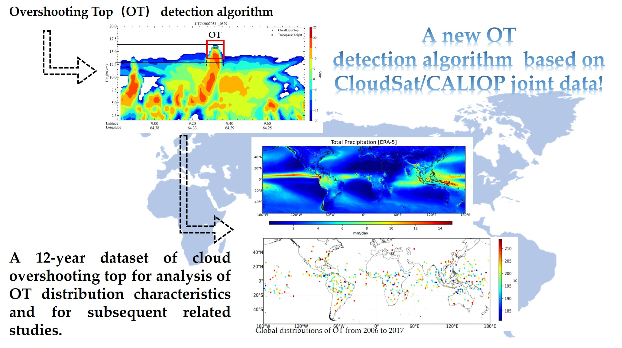
As introduced in Section 2, four different joint CloudSat/CALIOP products are used as the input of the new OT detection algorithm, including 2B-CLDCLASS-LIDAR, 2B-GEOPROF, MODIS-AUX, and ECMWF-AUX. The OT detection algorithm mainly includes three steps: calculating cloud top BT, calculating tropopause height, and identifying the OT samples.

After the initialization of the OT detection algorithm, the BT at MODIS channel 31 (11.05 μm, one of the atmospheric split-window channels) at the cloud top is calculated by using the matched radiance from the MODIS-AUX product, which can represent the cloud top height. The Planck formula is used here to calculate BT as follows:

$$\begin{gathered} c_1=2\pi {\mathrm{c}}^{2}h=3.7427\times {10}^8 \mathrm{W}•{\mathsf{\mu }\mathrm{m}}^{{}^4}•{\mathrm{m}}^{-2} \\ {c}_{{}_2}=\frac{ch}{k}=14,388 \mathsf{\mu }\mathrm{m}•K \\ T=\frac{c_{{}_2}}{\lambda }{\left(\ln \left(\frac{c_1}{B_{\left(\lambda ,T\right)}\pi {\lambda }^5}+1\right)\right)}^{-1} \end{gathered}$$

(1)

B_(λ,T) is the radiance observed by the satellite imaging sensor. In the c₁ and c₂ equations, c is the light speed, h is the Planck constant, and k is the Boltzmann constant.

After the BT calculation step, the matched atmospheric profile data from the ECMWF-AUX product is used to calculate the tropopause height. The tropopause is defined as “the lowest level at which the temperature lapse rate decreases to 2 °C/km or less, provided that the average lapse rate between this level and all higher levels within 2 km does not exceed 2 °C/km” (from the World Meteorological Organization). Assuming that the air temperature (T) varies linearly with pressure (P), the algorithm will use the temperature lapse rate less than the critical value (2 °C/km) at the tropopause, the hydrostatic equation, the state equation of ideal gas and the pressure at the tropopause to calculate tropopause height [37].

The final step of the algorithm is to identify the OT pixels. Previous studies have pointed out that the OT is an isolated area penetrating the tropopause with a much lower temperature than the surrounding anvil clouds [19]. To further highlight this feature of OT, the pixels with the BT at the MODIS 11.05 μm larger than 225 K are screened out at first. However, according to the results from this BT test, we have found many misjudged OT samples. Thus, the BT threshold is gradually adjusted to 214 K in the final test algorithm.

In addition to the three steps mentioned above, we also set some other thresholds to further eliminate the false OT candidates in the algorithm. The 2B-CLDCLASS-LIDAR dataset divides the clouds into 10 vertical layers with different types. Before the various physical properties of the cloud layer are determined, the deep convective cloud (DCC) of the highest cloud layer is selected. As the underlying surface has a substantial impact on the DCC intensity, the DCC samples are more easily detected over the land than over the ocean [38]. Therefore, the samples over the land and over the ocean should be treated separately in this step (Figure 1). The specific thresholds for discrimination over the ocean are different from those over the land. Therefore, the classification is conducted to avoid missing some important OT samples. To ensure that the OT candidates have a certain vertical thickness, the test thresholds are set with the requirement that the cloud geometry thickness should be more than 8 km and the cloud top height should be more than 12 km for all the samples. In addition, for the samples over the ocean, the test thresholds are set with the requirement that the cloud body thickness plus the altitude should be more than 10 km. Additionally, as the OT is an isolated area above the surrounding anvil clouds, we require that the highest cloud top should be 500 m higher than the surrounding cloud within 0.2 latitudes or longitudes around the potential OT sample along the CloudSat orbit [21].

Moreover, after these eliminating tests, the rest of the potential OT samples are filtered by requiring the radar echo averaged from the OT candidate layer to the next two layers exceeding −17 dBZ. Actually, the cumulus cloud with maximum radar echo > −15 has been discussed in previous studies [39]. The last step is that the surrounding cloud clusters must keep a certain thickness, and their BT must be below a specific value. Thus, the algorithm also sets the cloud thickness and BT thresholds for the surrounding cloud clusters within 0.2° latitudes or longitudes around the potential OT sample along the CloudSat orbit.

3.2. The Identified OT Samples

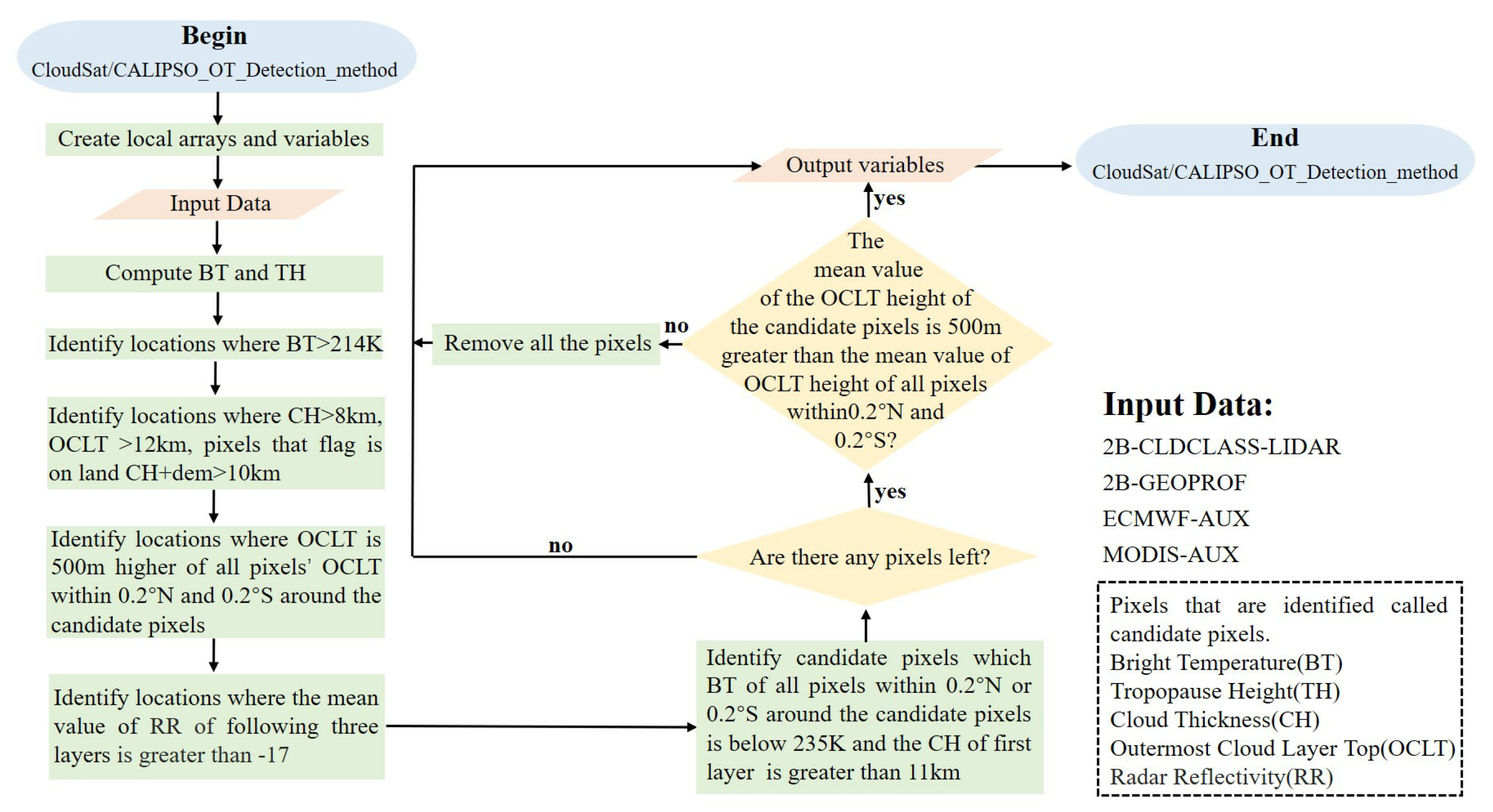
After identifying the OT samples along the CloudSat orbit, the corresponding latitude, longitude, BT, cloud top height, and tropopause height of each sample are written out to generate a new OT dataset, which can be used as a validation dataset for geostationary satellite algorithms in the future. Based on the joint CloudSat/CALIOP data from 2006 to 2017 (12 years), 549 OT samples around the globe are identified. Then, 28 misidentified samples are manually eliminated. As a result, 421 OT samples are obtained. Figure 2 shows the identified OT samples with radar echo cross-section data along the CloudSat orbit at 05:50 UTC on 16 September 2008. The identified OT samples and the matched radar echo image show that the OT samples look like a cauliflower-like tower, indicating the good performance of this new OT detection algorithm.

4. Results Analysis and Validation

4.1. Results

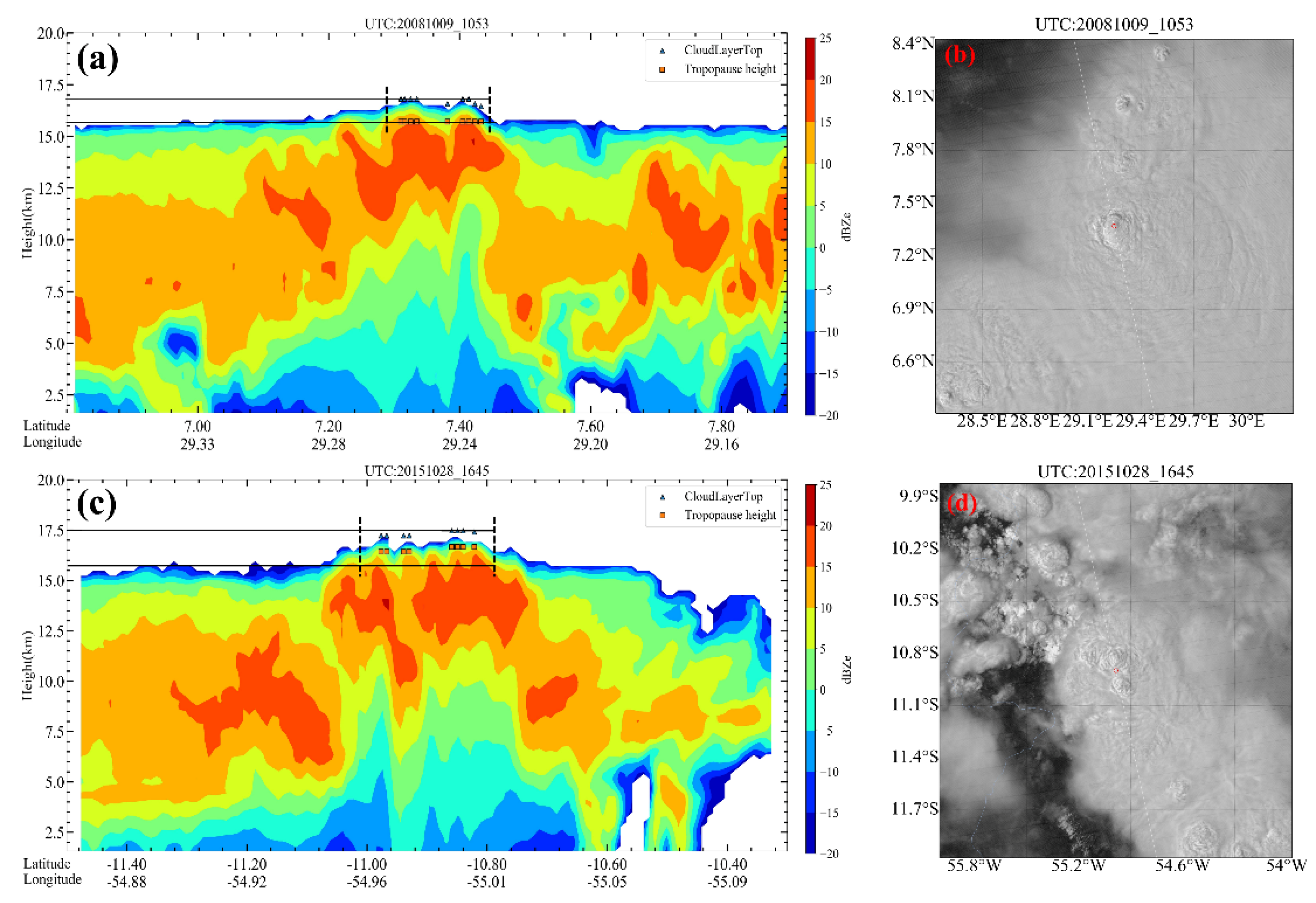
The OTs over different underlying surfaces have different characteristics, so the OTs over ocean and land are shown separately. Figure 3 shows two OT cases over land and the cloud images at the corresponding time. The case in Figure 3a occurred over the central African continent at 10:53 UTC on 9 October 2008. The radar echo image shows that the OT pixels identified by the new algorithm are evenly distributed in the protruding parts of the cloud cross-section. The cloud top height reaches 16.5 km, and the tropopause height reaches around 15.5 km. The cloud top is 1 km higher than the tropopause. There are strong radar echoes below the OT area. The cloud top height of the surrounding anvil cloud reaches about 15.5 km. Its distribution is relatively continuous, and it has a certain horizontal scale. The echo is in a block shape with smooth edges, indicating that the internal structure of the cloud is compact and the volume is huge. This conclusion can be confirmed by the visible cloud image at the corresponding time (Figure 3b). The MODIS orbit in the figure coincides with the OT area. The red circle in the figure corresponds to a protrusion obviously higher than the surrounding cloud anvil, roughly in 7.3°N–7.45°N, 29.23°E–29.27°E, which is consistent with the OT area identified by the algorithm on the radar echo image. Meanwhile, there is a uniform and huge anvil cloud distributed around the OT, which further proves that the algorithm can accurately recognize the OT. Another OT case over the land is presented in Figure 3c, which occurred at 16:45 UTC on 28 October 2015 over the center of South America. This OT case and related clouds share similar characteristics to the case in Figure 3a, indicating that the algorithm can accurately recognize OTs.

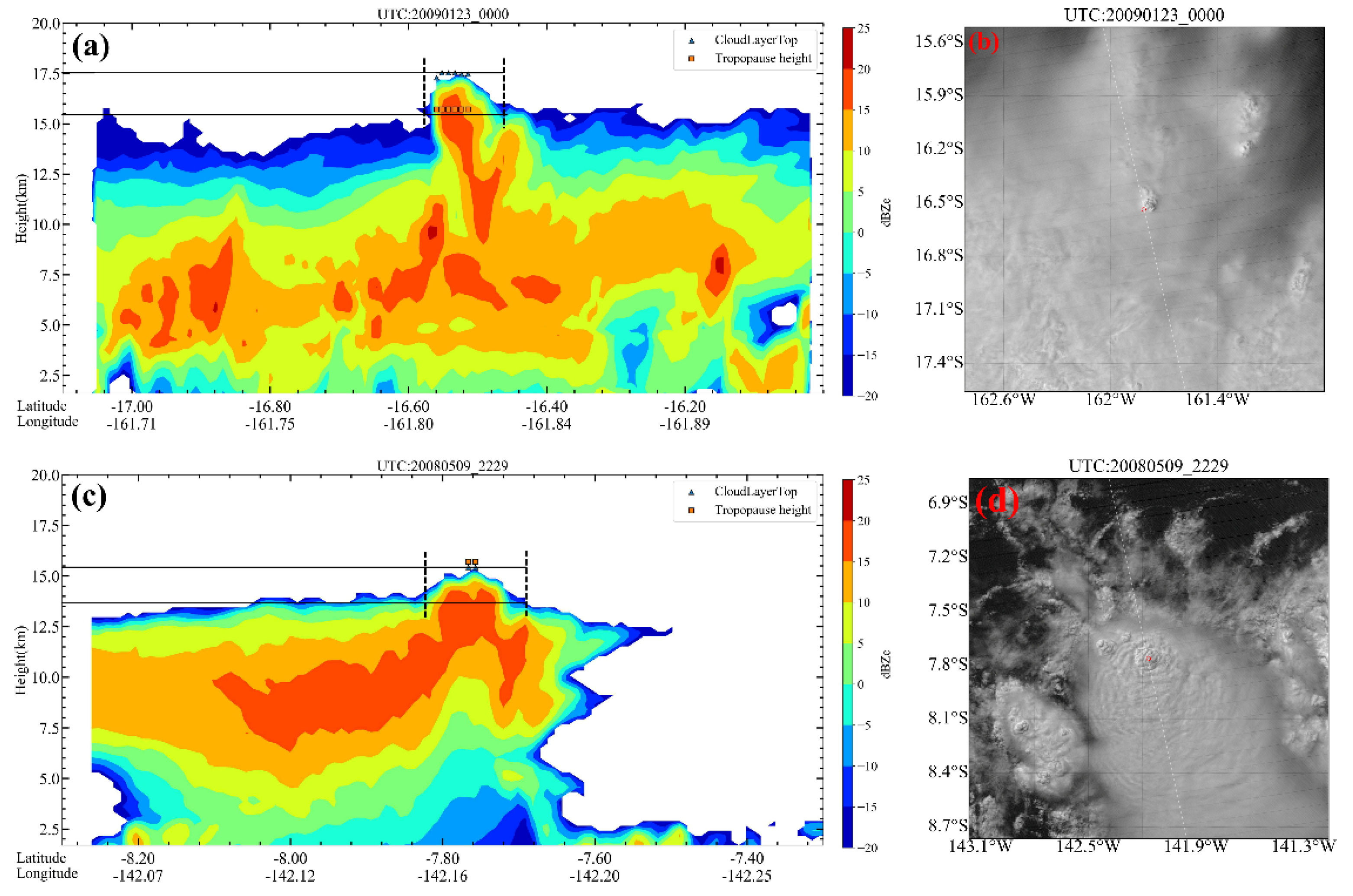
Figure 4 shows two OT cases over the ocean. The OT in Figure 4a occurred over the central Pacific Ocean at 00:00 UTC on 23 January 2009. The radar echo image shows that the OT pixels identified by the algorithm correspond well with the vertices of the cloud cross-section, and strong echoes exist in the OT area. The tropopause height is about 15.5 km, and the cloud top height is 17.5 km, 2 km higher than the tropopause. There is a wide weak echo area at the anvil cloud area on both sides of OT pixels, with no obvious boundaries. It is speculated that it is thin cirrus cloud or stratus cloud. The cloud top height of the anvil cloud is about 12.5 km, and the echo presents a large block area. The MODIS 250 m visible satellite image at the corresponding time (Figure 4b) shows that there is an obvious prominent cloud top at the red circle mark, and the range of the cloud top can well correspond to the OT area recognized by the algorithm. A light, thin cirrus cloud spreads around the protruding cloud top, and below the cirrus cloud is a huge anvil cloud extending towards high latitudes, which is also highly consistent with the cloud around OT in the echo image. It shows that the algorithm can accurately recognize the OT. The OT in Figure 4c occurred over the central Pacific Ocean at 22:29 on 9 May 2008. The radar echo image and the corresponding cloud image both show obvious OT characteristics, and the two images correspond well to each other. It is noteworthy that in this OT event, the OT height does not exceed the tropopause, and this phenomenon can appear both over the land and over the ocean. It indicates that whether a pixel is an OT pixel cannot be decided by the height difference between OT pixels and tropopause. Otherwise, many important OT samples would be missed. Even if the cloud top does not penetrate the tropopause, the convective cloud might be accompanied by OT.

The statistics of OT events in the dataset reveal that the OT cases over the land usually correspond to higher cloud top height, and the cloud top can often penetrate the tropopause, indicating that the OT over the land always has higher intensity. Some OT cases with the cloud top height lower than the tropopause exist in the dataset, such as the case shown in Figure 4c, indicating that the height difference between cloud top and tropopause cannot be used to judge whether a convective cloud is OT. Additionally, in the 28 eliminated cases, some of them are thin cirrus clouds which are misjudged as OT. Therefore, how to better distinguish these thin cirrus pixels from OT pixels should be considered in detail in the future improvement of the algorithm.

4.2. Spatio-Temporal Distribution Characteristics of OT

Figure 5 shows the global distribution of OTs in the dataset, and their accuracy has been checked by radar echo data image and the MODIS 250 m visible satellite image (when the image exists). It can be seen that OT events are mainly in the equatorial and low latitudes from 30°S to 30°N, especially in the areas south of China and north of Australia. The global solar radiation and heat are mainly concentrated in the equatorial and low latitude regions, which are mainly controlled by equatorial and tropical air masses. In this latitude range, the seasonal changes in climate are not obvious, the temperature is high throughout the year, and the diurnal temperature variation is greater than the annual temperature variation. Such characteristics lead to strong vertical motions in low latitudes, where strong convective weather often occurs in the afternoon. In the daytime, the ground is continuously heated by solar short wave radiation, and meanwhile, it emits longwave radiation to heat the atmosphere. The air on the surface is heated and expanded, and the air density is reduced, resulting in updrafts. After rising to a certain height, the heated updrafts begin to cool down, and the water vapor contained in the air begins to condense into water droplets. The small water droplets can grow in the strong updraft, and finally, the updraft cannot support their weight, and the water droplets fall to the ground. OT is the product of updraft in severe convective storms, which explains why OT mainly occurs in the equatorial and low latitude regions.

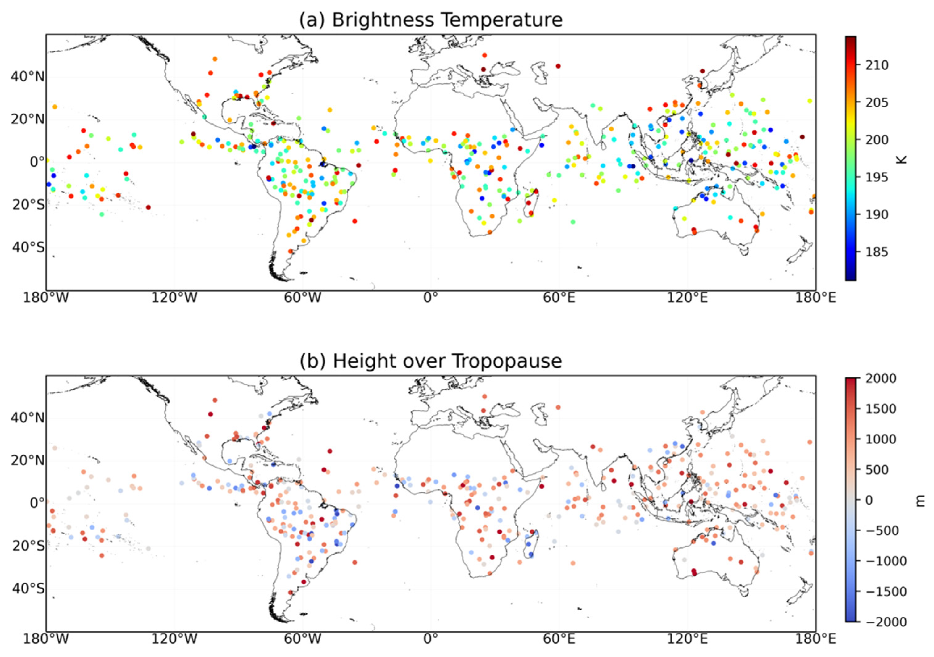
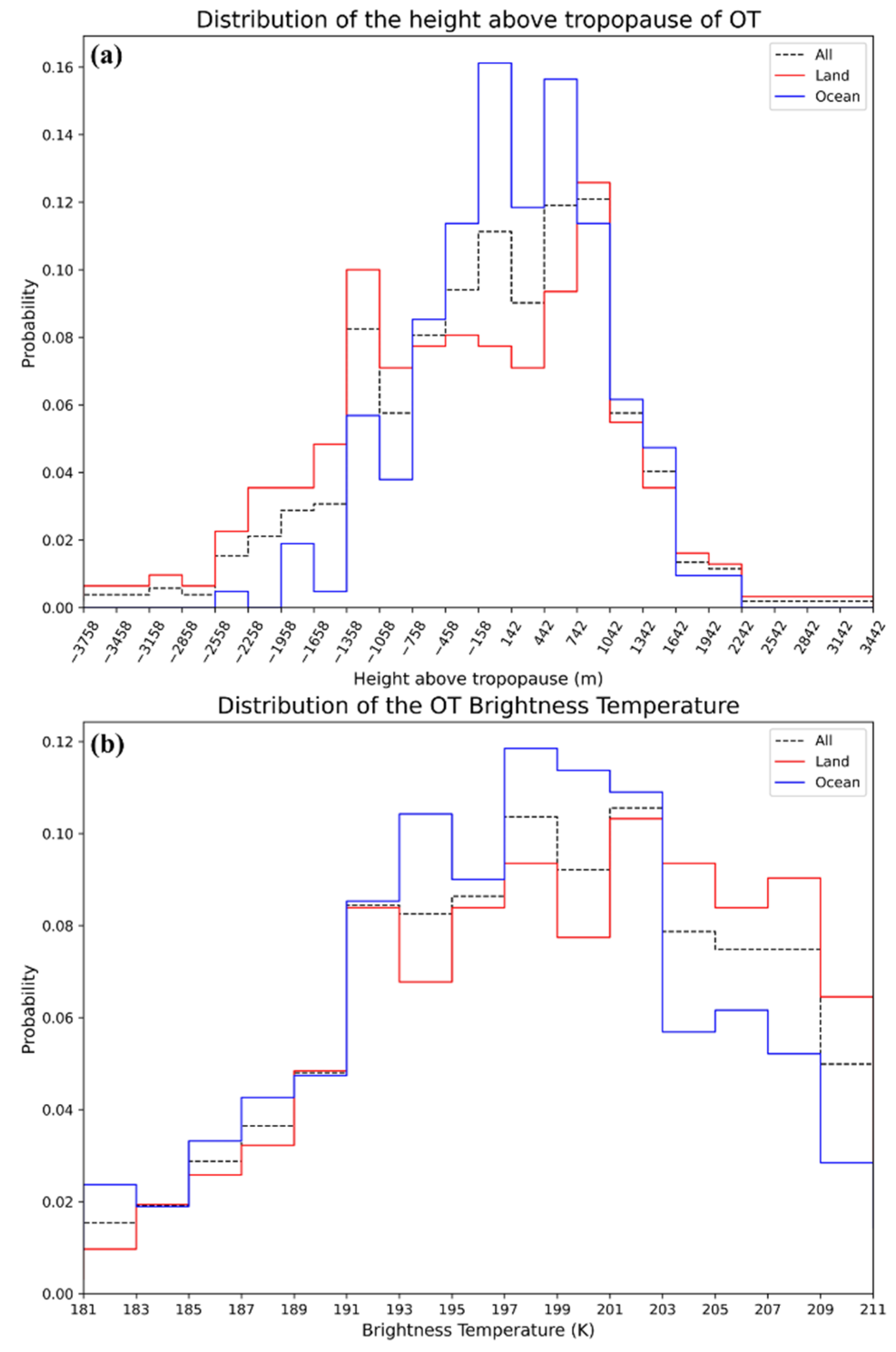
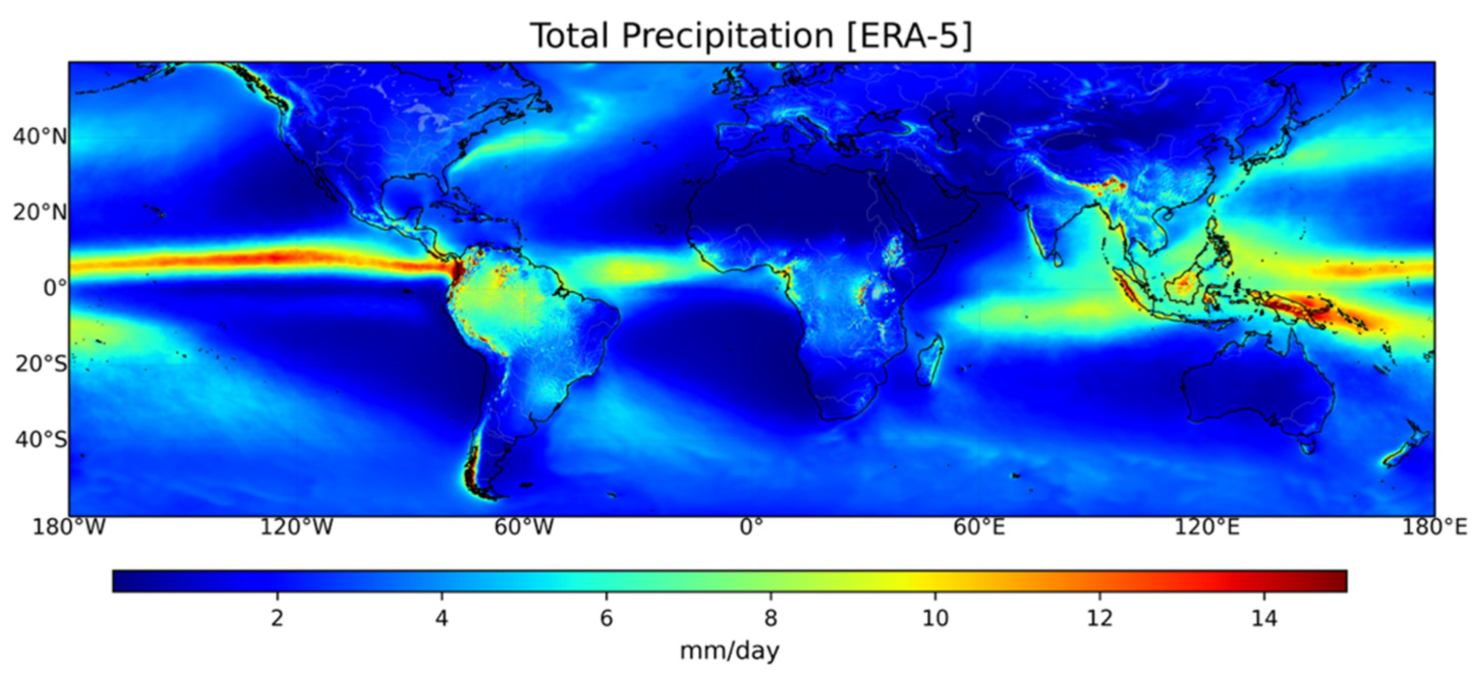
Figure 5a shows the distribution of average BT in the OT area. It can be seen that the OT events over the ocean are relatively warm. The average BT of OT area over the land is obviously lower than that over the ocean, and the BT of OT in inland areas is also lower than that in coastal areas. The probability density distribution of BT in Figure 6b shows that the average BT of OT area is mostly within 190 K–209 K, with the probability peak appearing at about 200 K. Figure 5b shows the height difference between OT and the tropopause for the cases in the OT dataset. As can be seen, there is an obvious sea–land difference. The convection intensity over the land and coastal areas is greater than that over the ocean, so the OT over the land may penetrate the tropopause more often. Figure 5a,b shows that OT presents obviously different distribution characteristics over different underlying surfaces. On the whole, the OT over the land is obviously stronger than that over the ocean. It is mainly due to the fact that the convective effective potential energy over the land is much greater than that over the ocean in summer, and the atmospheric stratification is more unstable over the land. It is worth noting that the primary locations of OT samples concentrated are in line with the global distribution of average precipitation (see Figure 5 and Figure 7). The gridded data in Figure 7 are from ERA-5, the fifth-generation reanalysis dataset on global weather and climate released by the European Centre for Medium-range Weather Forecasts (ECMWF), which show the higher spatial and temporal resolutions (hourly and 0.25° × 0.25°), the better global balance of precipitation, and evaporation compared to the previous ERA-Interim atmospheric reanalysis [40].

Figure 6a shows that the height difference between OT and tropopause is mostly within 700–1000 m. The probability distribution of the height difference between OT and tropopause over the land presents double peaks at about −1200 m and 800 m. However, it shows a single peak for the OTs over the ocean, and the peak appears within −100–700 m. In general, the height difference between the OT and tropopause is within 700–1000 m, indicating that most OT cloud tops can penetrate the tropopause. The analysis reveals that an OT event is most likely to occur when the average BT of convective cloud top is about 200 K, and the average height difference is 700–1000 m.

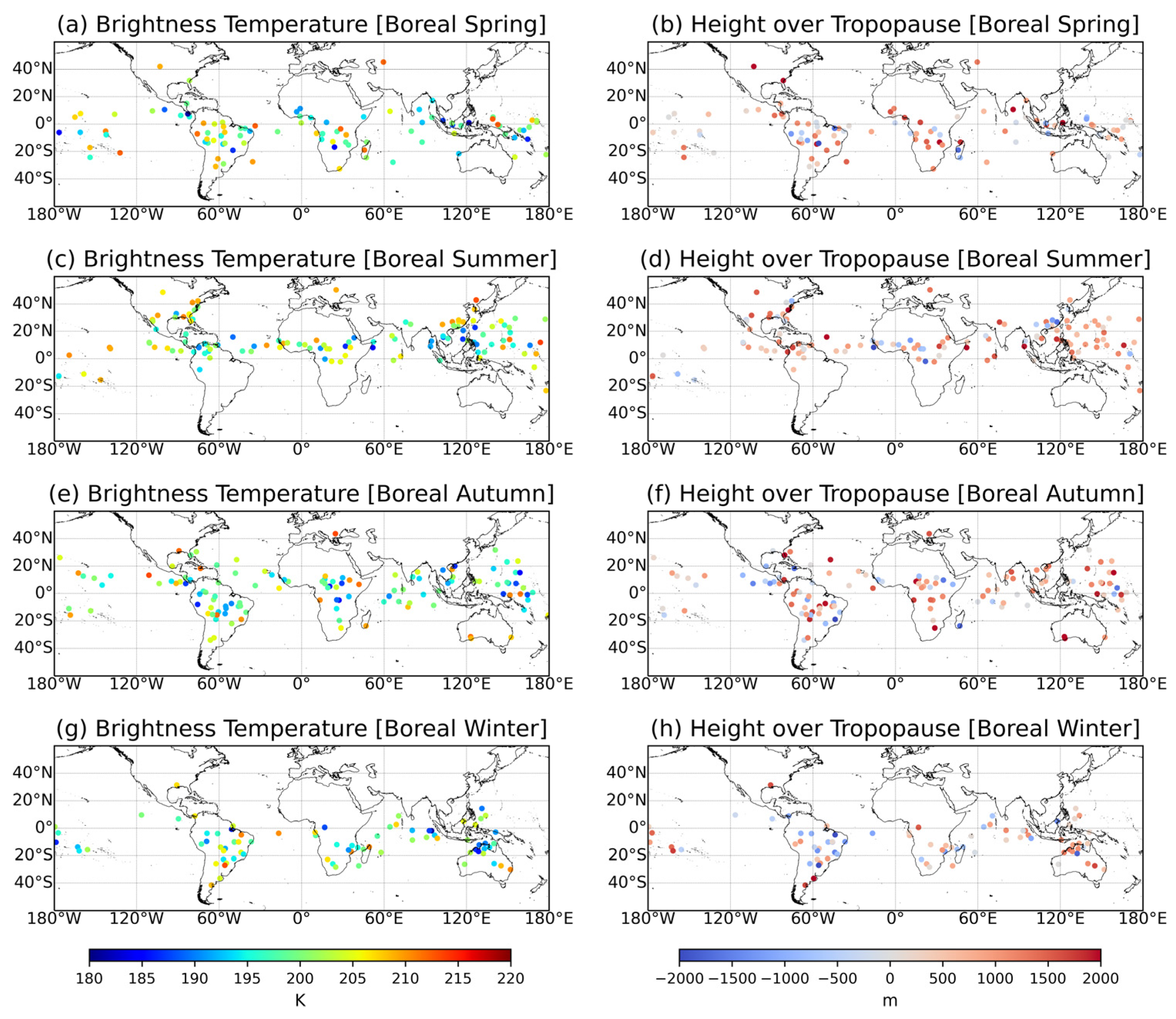
Figure 8 shows the distribution of OT brightness temperature and the height difference of all OT events in the dataset in different seasons in the Northern Hemisphere. It can be seen that OT events are mainly distributed in the equatorial and low latitude regions in all four seasons in the Northern Hemisphere, with the lowest frequency in boreal winter. In boreal summer, OT events are densely distributed over both the land and the ocean in low latitude areas near the equator. In boreal autumn and boreal winter, OT events are mainly distributed over the land and less over the ocean. The average BT of OT over the inland areas is lower than that over the ocean throughout the year, and that over the inland areas is lower than that over coastal areas. The OT with lower BT corresponds to the large height difference between OT and tropopause in the figure, indicating that the BT of OT is inversely proportional to the convection intensity. The lower the average BT in the OT area is, the stronger the convection that triggers OT is. The height difference is greater over the land than over the ocean throughout the year, which confirms again that the convection intensity is greater over the land than over the ocean. Meanwhile, in all seasons in the Northern Hemisphere, there are some OT cases with heights lower than the tropopause height, indicating the previous conclusion that the positive height difference is not a must condition for OT identification. The Northern Hemisphere seasonal differences in height difference show that the convection development is most vigorous in boreal summer when the height of OT is much larger than the height of the tropopause. It is noteworthy that there is some highly developed convection in the western Pacific as well, and the intensity is not lower than that of OT over the land.

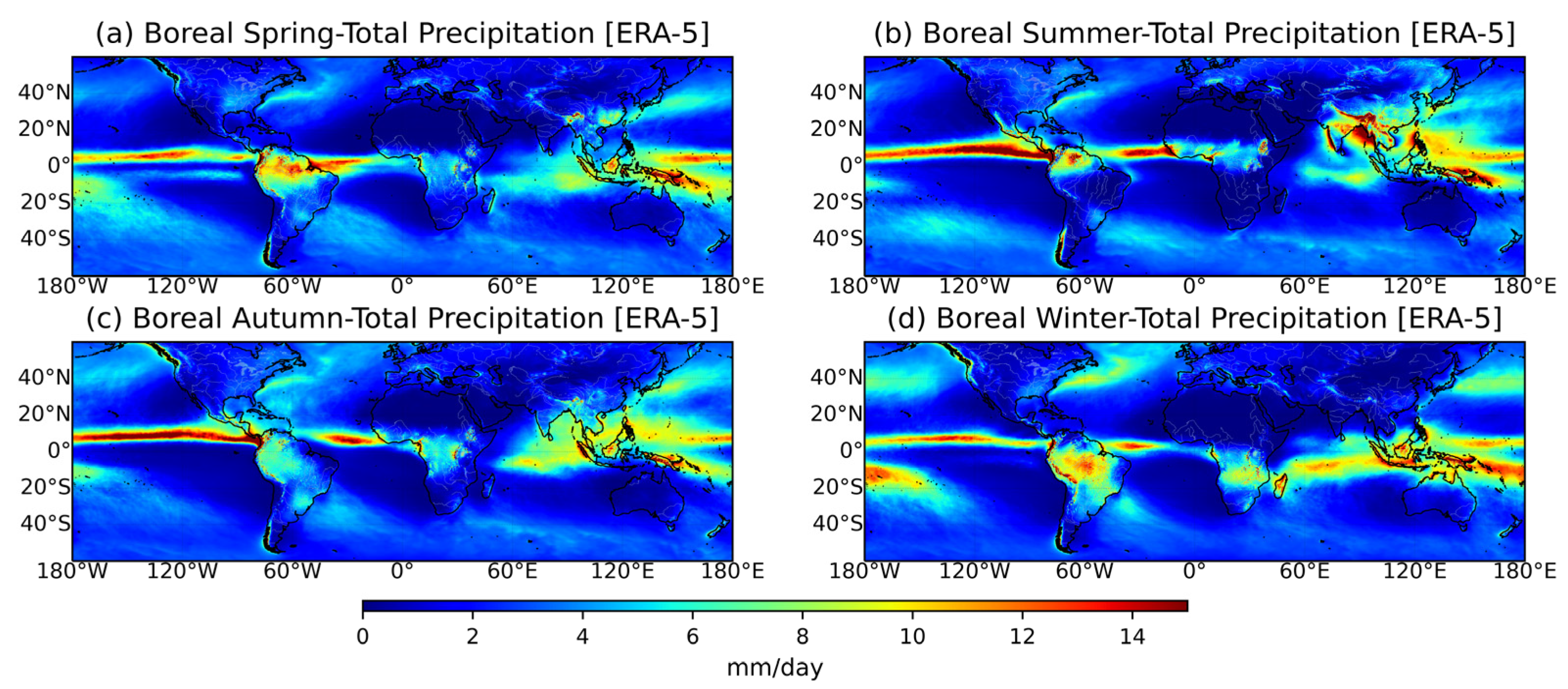
In addition, it finds a significant seasonal shift in the horizontal distribution of OT samples in the north–south direction (or along the latitude) of the Northern Hemisphere in Figure 8, while this seasonal shift is the most obvious in boreal summer. In Figure 8, the locations of OT distribution in boreal spring and boreal autumn are near the equator, but it moves northward manifestly in boreal summer (0°N~40°N) and slightly southward in boreal winter (0°S~40°S) (compared with boreal spring and boreal autumn). This seasonal shift of OT in the Northern Hemisphere from this investigation is consistent with the seasonal average precipitation distribution (representing rain band) from 2006 to 2017, shown in Figure 9. It is not surprising that the seasonal shift of OT in the Northern Hemisphere around the equator is also synchronous and associated with the Inter-Tropical Convergence Zone (ITCZ), which is the result of the atmospheric circulation system and the planetary zonal wind system. This finding also indicates the close connection of OT with severe weather mentioned in the introduction section [8].

5. Discussion

In this study, we introduce a new 12-year OT detection algorithm based on CloudSat/CALIOP joint observation data. According to the definitions of OT, we identify the OT samples by using the features of OT and the distribution of BT. Considering the difference in deep, convective clouds over the land and over the ocean, the algorithm processes the OT samples over the land and over the ocean separately. Over the 12 years, a total of 549 OT samples from all over the world are output by the algorithm.

Then, we verify the accuracy of the new OT detection algorithm through manual screening. We first use the radar echo image to check whether the identified OT pixels match the cloud top area, and then we use the MODIS 250 m visible satellite image to verify the accuracy and feasibility of the algorithm again. After verification, 28 misjudged samples are removed, and an OT dataset containing 521 samples is generated (the dataset can be obtained by contacting the author Min Min via [email protected]). Further verification of the OT dataset shows that the OT pixels identified by the algorithm are highly consistent with features of OT on the visible satellite image, which verifies the accuracy and stability of the algorithm.

6. Conclusions

On the basis of this OT dataset, the features and spatio-temporal distribution characteristics of OT events are analyzed in detail. The main conclusions are as follows:

(1) The statistical analysis of the OT dataset shows that the OT over the land is stronger than that over the ocean. The OT cases are mainly concentrated in equatorial and middle latitude regions (within 60°) with an obvious seasonal distribution deviation. The lower average BT of the OT samples corresponds to the larger height difference between the OT and tropopause, indicating that the BT of OT is inversely proportional to the intensity of OT, and the lower BT corresponds to the higher OT intensity. Furthermore, boreal summer (boreal winter) has the highest (lowest) OT frequency. Meanwhile, the analysis of the probability density distribution of the BT in the OT area and the height difference between OT and tropopause shows that when the average BT of the cloud top is about 200 K and the height difference is 700–1000 m, OT is most likely to occur.

(2) Most previous studies on OT are based on the observation data of satellite passive remote sensing, and there have been no statistics on the spatio-temporal distribution characteristics of OT in a long time series. In this study, the joint observation data based on active remote sensing is used to accurately identify the OT samples and generate a set of high-precision OT data. By summarizing and analyzing the distribution characteristics and occurrence law of OT, we can better understand the climatic characteristics of global OT.

(3) We also use this dataset to further reveal the synchronously seasonal shift of OT and rain bands in the north–south direction near the equator in the Northern Hemisphere, implying the possible close relationship between the occurrence of OT and severe weather events on a global scale.

References

- Hoeppe, P. Trends in weather related disasters-Consequences for insurers and society. Weather Clim. Extremes 2016, 11, 70–79. [Google Scholar] [CrossRef] [Green Version]
- Negri, A.J.; Adler, R.F. Relation of Satellite-Based Thunderstorm Intensity to Radar-Estimated Rainfall. J. Appl. Meteorol. Climatol. 1981, 20, 288–300. [Google Scholar] [CrossRef] [Green Version]
- Hung, R.; Smith, R. Satellite infrared imagery, rawinsonde data, and gravity wave remote sensing of severe convective storms. Int. J. Infrared Milli. 1982, 3, 489–502. [Google Scholar] [CrossRef]
- Marion, G.R.; Trapp, R.J.; Nesbitt, S.W. Using Overshooting Top Area to Discriminate Potential for Large, Intense Tornadoes. Geophys. Res. Lett. 2019, 46, 12520–12526. [Google Scholar] [CrossRef]
- Ziegler, C.L.; Macgorman, D.R. Observed Lightning Morphology Relative to Modeled Space Charge and Electric Field Distributions in a Tornadic Storm. J. Atmos. Sci. 1994, 51, 833–851. [Google Scholar] [CrossRef]
- Heymsfield, G.M.; Fulton, R.; Spinhirne, J.D. Aircraft Overflight Measurements of Midwest Severe Storms: Implications an Geosynchronous Satellite Interpretations. Mon. Weather Rev. 1991, 119, 436. [Google Scholar] [CrossRef]
- Reynolds, D.W. Observations of Damaging Hailstorms from Geosynchronous Satellite Digital Data. Mon. Weather Rev. 1980, 108, 337. [Google Scholar] [CrossRef]
- Bedka, K.M. Overshooting cloud top detections using MSG SEVIRI Infrared brightness temperatures and their relationship to severe weather over Europe. Atmos. Res. 2011, 99, 175–189. [Google Scholar] [CrossRef]
- Machado, L.; Lima, W.; Pinto, O., Jr.; Morales, C.A. Relationship between cloud-to-ground discharge and penetrative clouds: A multi-channel satellite application. Atmos. Res. 2009, 93, 304–309. [Google Scholar] [CrossRef]
- Berendes, T.A.; Mecikalski, J.R.; Mackenzie, W.M.; Bedka, K.M.; Nair, U.S. Convective cloud identification and classification in daytime satellite imagery using standard deviation limited adaptive clustering. J. Geophys. Res. Atmos. 2008, 113, D20207. [Google Scholar] [CrossRef] [Green Version]
- Bedka, K.M.; Khlopenkov, K. A Probabilistic Multispectral Pattern Recognition Method for Detection of Overshooting Cloud Tops Using Passive Satellite Imager Observations. J. Appl. Meteorol. Climatol. 2016, 55, 1983–2005. [Google Scholar] [CrossRef]
- Lindsey, D.T.; Grasso, L. An Effective Radius Retrieval for Thick Ice Clouds Using GOES. J. Appl. Meteorol. Climatol. 2008, 47, 1222. [Google Scholar] [CrossRef] [Green Version]
- Rosenfeld, D.; Woodley, W.L.; Lerner, A.; Kelman, G.; Lindsey, D.T. Satellite detection of severe convective storms by their retrieved vertical profiles of cloud particle effective radius and thermodynamic phase. J. Geophys. Res. Atmos. 2008, 113, D04208. [Google Scholar] [CrossRef] [Green Version]
- Fritz, S.; Laszlo, I. Detection of water vapor in the stratosphere over very high clouds in the tropics. J. Geophys. Res. Atmos. 1993, 98, 22959–22967. [Google Scholar] [CrossRef]
- Ackerman, S.A. Global Satellite Observations of Negative Brightness Temperature Differences between 11 and 6.7 µm. J. Atmos. Sci. 1996, 53, 2803–2812. [Google Scholar] [CrossRef] [Green Version]
- Schmetz, J.; Tjemkes, S.A.; Gube, M.; Berg, L. Monitoring deep convection and convective overshooting with METEOSAT. Adv. Space Res. 1997, 19, 433–441. [Google Scholar] [CrossRef]
- Jurkovic, P.M.; Mahovic, N.S.; Pocakal, D. Lightning, overshooting top and hail characteristics for strong convective storms in Central Europe. Atmos. Res. 2015, 161, 153–168. [Google Scholar] [CrossRef]
- Setvak, M.; Rabin, R.M.; Wang, P.K. Contribution of the MODIS instrument to observations of deep convective storms and stratospheric moisture detection in GOES and MSG imagery. Atmos. Res. 2007, 83, 505–518. [Google Scholar] [CrossRef]
- Bedka, K.; Brunner, J.; Dworak, R.; Feltz, W.; Otkin, J.; Greenwald, T. Objective satellite-based detection of overshooting tops using infrared window channel brightness temperature gradients. J. Appl. Meteorol. Climatol. 2010, 49, 181–202. [Google Scholar] [CrossRef]
- Brunner, J.C.; Ackerman, S.A.; Bachmeier, A.S.; Rabin, R.M. A quantitative analysis of the enhanced-V feature. Weather Forecast. 2007, 22, 853–872. [Google Scholar] [CrossRef]
- Negri, A.J. Cloud-top structure of tornadic storms on 10 April 1979 from rapid scan and stereo satellite observations. Bull. Am. Meteorol. Soc. 1982, 63, 1151–1159. [Google Scholar] [CrossRef] [Green Version]
- Adler, R.F.; Markus, M.J.; Fenn, D.D.; Szejwach, G.; Shenk, W.E. Thunderstorm top structure observed by aircraft overflights with an infrared radiometer. J. Appl. Meteorol. Climatol. 1983, 22, 579–593. [Google Scholar] [CrossRef] [Green Version]
- Bedka, K.M.; Minnis, P. GOES 12 observations of convective storm variability and evolution during the Tropical Composition, Clouds and Climate Coupling Experiment field program. J. Geophys. Res. Atmos. 2010, 115, D00J13. [Google Scholar] [CrossRef]
- Punge, H.; Bedka, K.; Kunz, M.; Werner, A. A new physically based stochastic event catalog for hail in Europe. Nat. Hazards 2014, 73, 1625–1645. [Google Scholar] [CrossRef]
- Dworak, R.; Bedka, K.; Brunner, J.; Feltz, W. Comparison between GOES-12 overshooting-top detections, WSR-88D radar reflectivity, and severe storm reports. Weather Forecast. 2012, 27, 684–699. [Google Scholar] [CrossRef] [Green Version]
- Bedka, K.M.; Dworak, R.; Brunner, J.; Feltz, W. Validation of Satellite-Based Objective Overshooting Cloud-Top Detection Methods Using CloudSat Cloud Profiling Radar Observations. J. Appl. Meteorol. Climatol. 2012, 51, 1811–1822. [Google Scholar] [CrossRef]
- Gettelman, A.; Salby, M.; Sassi, F. Distribution and influence of convection in the tropical tropopause region. J. Geophys. Res. Atmos. 2002, 107, ACL 6-1–ACL 6-12. [Google Scholar] [CrossRef]
- Dessler, A.E. The effect of deep, tropical convection on the tropical tropopause layer. J. Geophys. Res. Atmos. 2002, 107, ACH 6-1–ACH 6-5. [Google Scholar] [CrossRef] [Green Version]
- Wang, P.K. Moisture plumes above thunderstorm anvils and their contributions to cross-tropopause transport of water vapor in midlatitudes. J. Geophys. Res. Atmos. 2003, 108, 4194. [Google Scholar] [CrossRef] [Green Version]
- Wang, P.K.; Setvák, M.; Lyons, W.; Schmid, W.; Lin, H.M. Further evidences of deep convective vertical transport of water vapor through the tropopause. Atmos. Res. 2009, 94, 400–408. [Google Scholar] [CrossRef]
- Riehl, H.; Malkus, J.S. On the heat balance in the equatorial trough zone. Geophysica 1958, 6, 503–538. [Google Scholar]
- Jiang, J.H.; Livesey, N.J.; Su, H.; Neary, L.; Mcconnell, J.C.; Richards, N. Connecting surface emissions, convective uplifting, and long-range transport of carbon monoxide in the upper troposphere: New observations from the Aura Microwave Limb Sounder. Geophy. Res. Lett. 2007, 34, 312–321. [Google Scholar] [CrossRef] [Green Version]
- Takahashi, H.; Luo, Z.J. Characterizing tropical overshooting deep convection from joint analysis of CloudSat and geostationary satellite observations. J. Geophys. Res. Atmos. 2014, 119, 112–121. [Google Scholar] [CrossRef]
- Kaltenböck, R.; Diendorfer, G.; Dotzek, N. Evaluation of thunderstorm indices from ECMWF analyses, lightning data and severe storm reports. Atmos. Res. 2009, 93, 381–396. [Google Scholar] [CrossRef] [Green Version]
- Kerr-Munslow, A.M.; Norton, W.A. Driving of The Annual Cycle In Lower-stratospheric Tropical Temperatures By Localised Breaking of Synoptic-scale Waves. In Proceedings of the EGS General Assembly Conference Abstracts, Nice, France, 21–26 April 2002. [Google Scholar]
- Setvák, M.; Bedka, K.; Lindsey, D.T.; Sokol, A.; Charvát, Z.; Šťástka, J.; Wang, P.K. A-Train observations of deep convective storm tops. Atmos. Res. 2013, 123, 229–248. [Google Scholar] [CrossRef]
- Reichler, T. Determining the tropopause height from gridded data. Geophy. Res. Lett. 2003, 30, ASC6-1–ASC6-5. [Google Scholar] [CrossRef] [Green Version]
- Jorgensen, D.P.; LeMone, M.A. Vertically Velocity Characteristics of Oceanic Convection. J. Atmos. Sci. 1989, 46, 621–640. [Google Scholar] [CrossRef] [Green Version]
- L’Ecuyer, T.S.; Berg, W.; Haynes, J.; Lebsock, M.; Takemura, T. Global observations of aerosol impacts on precipitation occurrence in warm maritime clouds. J. Geophys. Res. Atmos. 2009, 114, D09211. [Google Scholar] [CrossRef] [Green Version]
- Albergel, C.; Dutra, E.; Munier, S.; Calvet, J.-C.; Munoz-Sabater, J.; de Rosnay, P.; Balsamo, G. ERA-5 and ERA-Interim driven ISBA land surface model simulations: Which one performs better? Hydrol. Earth Syst. Sci. 2018, 22, 3515–3532. [Google Scholar] [CrossRef] [Green Version]
Figure 1.
Flowchart of OT detection algorithm based on CloudSat/CALIOP joint data.
Figure 2.
Identified OT samples along the CloudSat orbit at 05:50 UTC on 16 September 2008. The colormap represents the radar echo of CloudSat.
Figure 3.
(a,c) OT samples in the CloudSat radar echo cross-section and (b,d) the MODIS 250 m visible satellite images over the land at 10:53 UTC on 9 October 2008 (top panels) and at 16:45 UTC on 28 October 2015 (bottom panels).
Figure 4.
Same as Figure 3, except for the OT samples over the ocean at 00:00 UTC on 23 January 2009 (top panels) and at 22:29 UTC on 9 May 2008 (bottom panels).
Figure 5.
Global distributions of brightness temperature of identified OT samples (a) and the height over corresponding tropopause (b) from 2006 to 2017.
Figure 6.
Probability density function of height difference between OT and the tropopause (a) and brightness temperature (b).
Figure 7.
Global distribution of average total precipitation (mm/day) from 2006 to 2017 using ERA-5.
Figure 8.
Seasonal distributions of brightness temperature (left panels) and height difference between OT and tropopause (right panels) for identified OT samples from 2006 to 2017. (a,b) are for boreal spring (MAM), (c,d) are for boreal summer (JJA), (e,f) are for boreal autumn (SON), and (g,h) are for boreal winter (DJF).
Figure 9.
Same as Figure 7, but for the results of (a) boreal spring (MAM), (b) boreal summer (JJA), (c) boreal autumn (SON), and (d) boreal winter (DJF).
Publisher’s Note: MDPI stays neutral with regard to jurisdictional claims in published maps and institutional affiliations. |
© 2022 by the authors. Licensee MDPI, Basel, Switzerland. This article is an open access article distributed under the terms and conditions of the Creative Commons Attribution (CC BY) license (https://creativecommons.org/licenses/by/4.0/).
Share and Cite
MDPI and ACS Style
Li, H.; Wei, X.; Min, M.; Li, B.; Nong, Z.; Chen, L. A Dataset of Overshooting Cloud Top from 12-Year CloudSat/CALIOP Joint Observations. Remote Sens. 2022, 14, 2417. https://0-doi-org.brum.beds.ac.uk/10.3390/rs14102417
AMA Style
Li H, Wei X, Min M, Li B, Nong Z, Chen L. A Dataset of Overshooting Cloud Top from 12-Year CloudSat/CALIOP Joint Observations. Remote Sensing. 2022; 14(10):2417. https://0-doi-org.brum.beds.ac.uk/10.3390/rs14102417
Chicago/Turabian StyleLi, Haoyang, Xiaocheng Wei, Min Min, Bo Li, Ziqi Nong, and Lin Chen. 2022. "A Dataset of Overshooting Cloud Top from 12-Year CloudSat/CALIOP Joint Observations" Remote Sensing 14, no. 10: 2417. https://0-doi-org.brum.beds.ac.uk/10.3390/rs14102417
Note that from the first issue of 2016, this journal uses article numbers instead of page numbers. See further details here.