
A Morphological Feature-Oriented Algorithm for Extracting Impervious Surface Areas Obscured by Vegetation in Collaboration with OSM Road Networks in Urban Areas


Abstract
: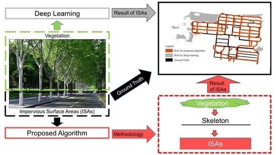
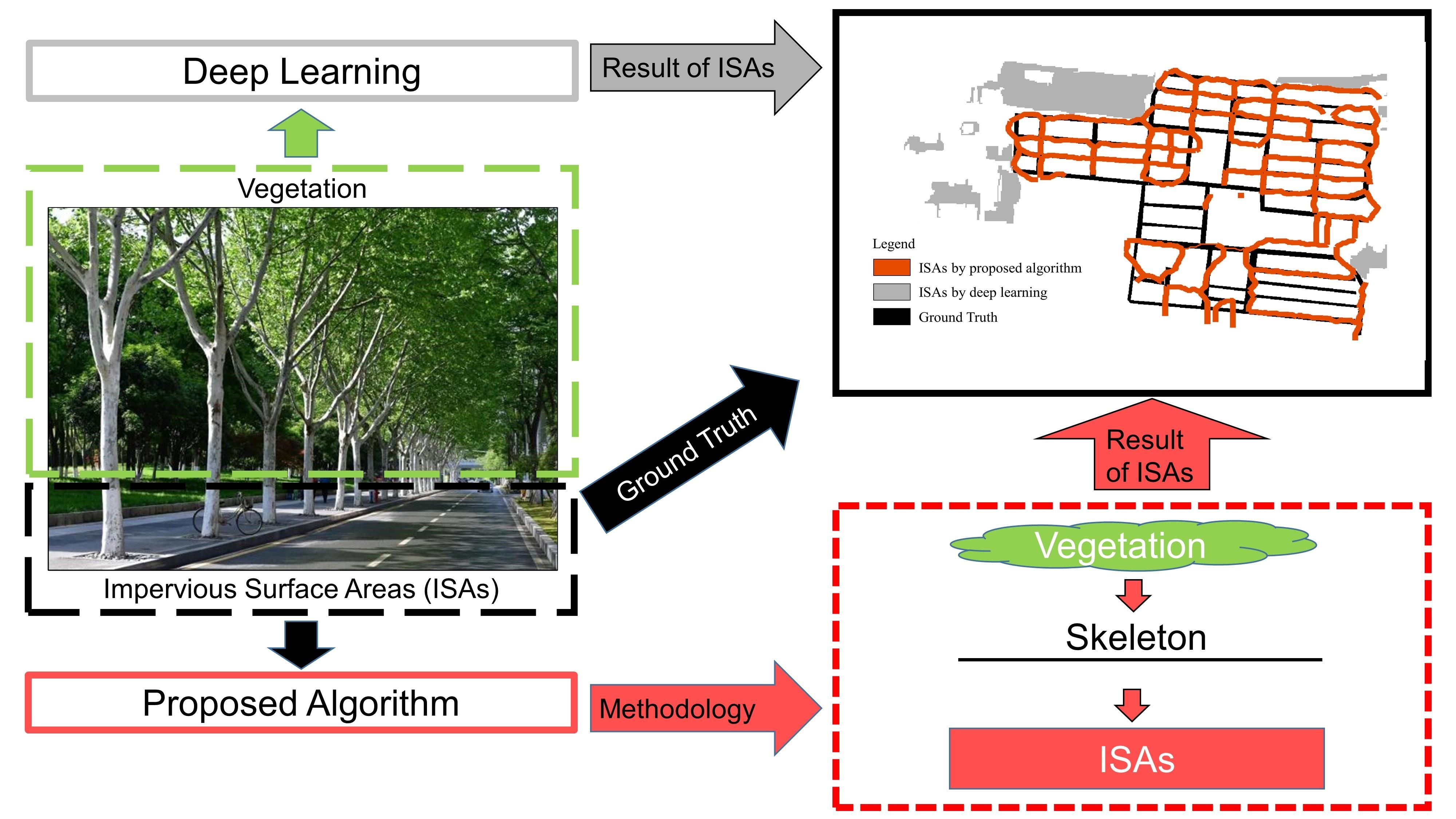
1. Introduction
2. Study Area and Data Used
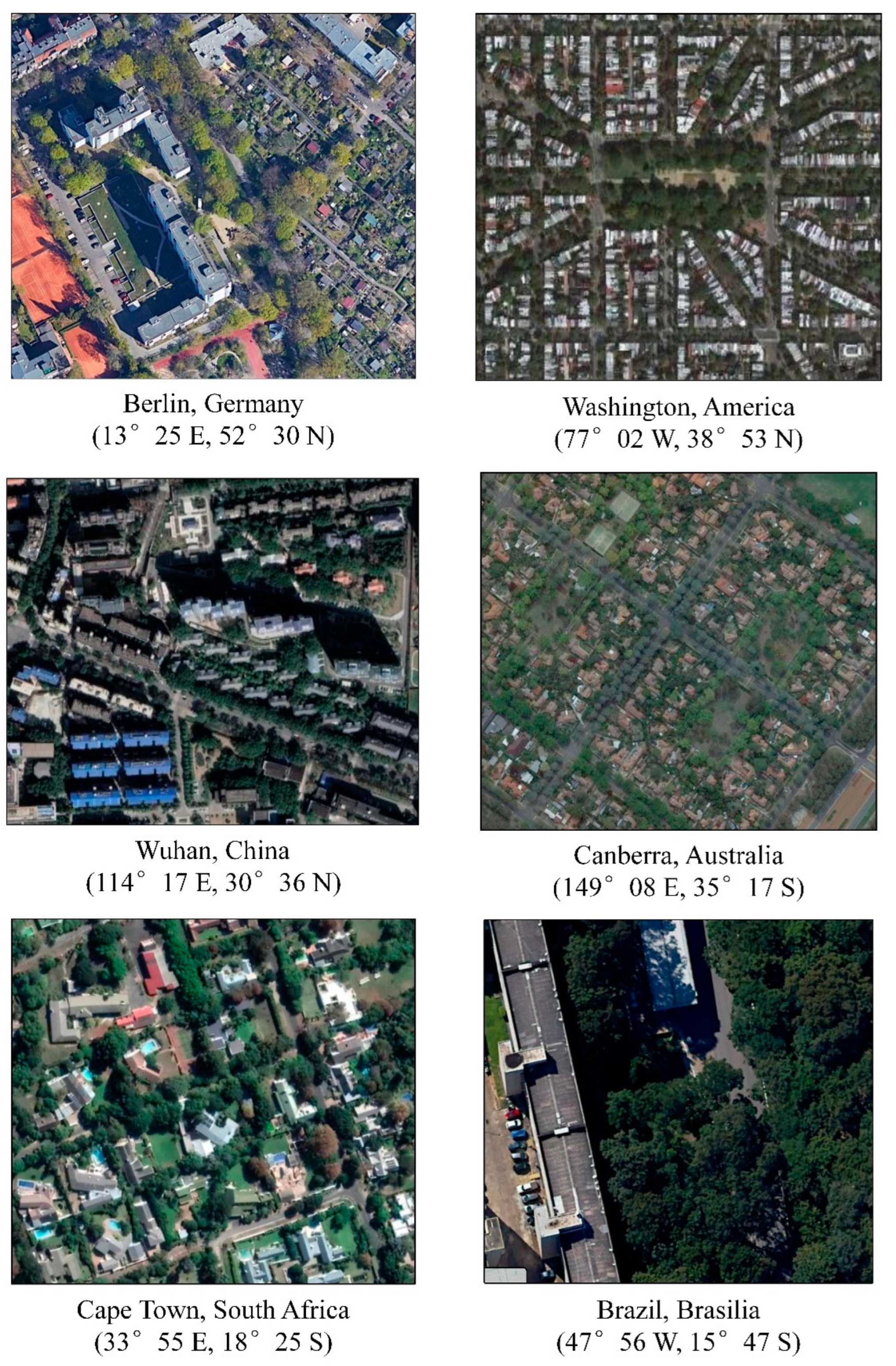
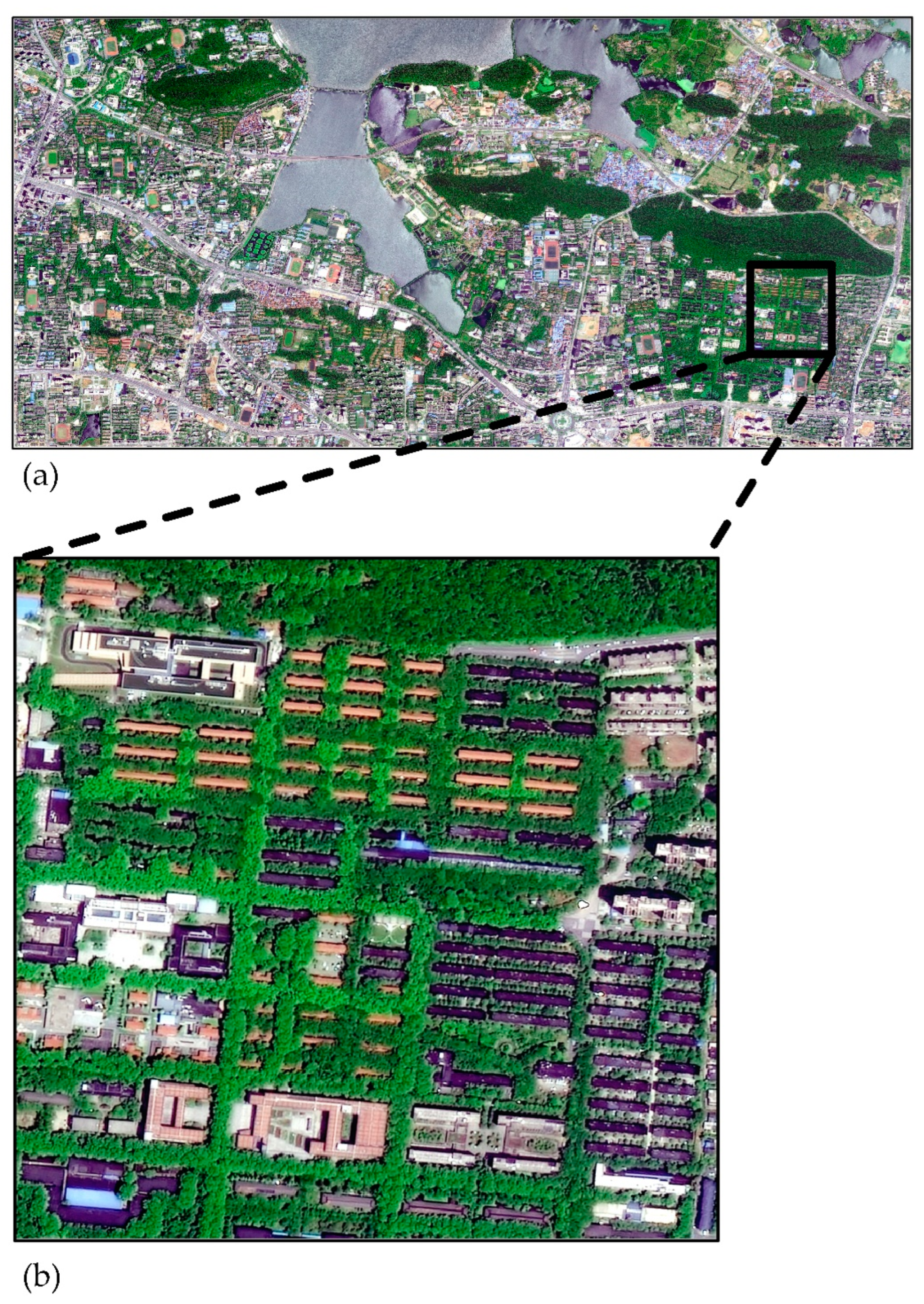
2.1. The Study Area
2.2. Data Used
2.2.1. GF-2 Remotely Sensed Imagery
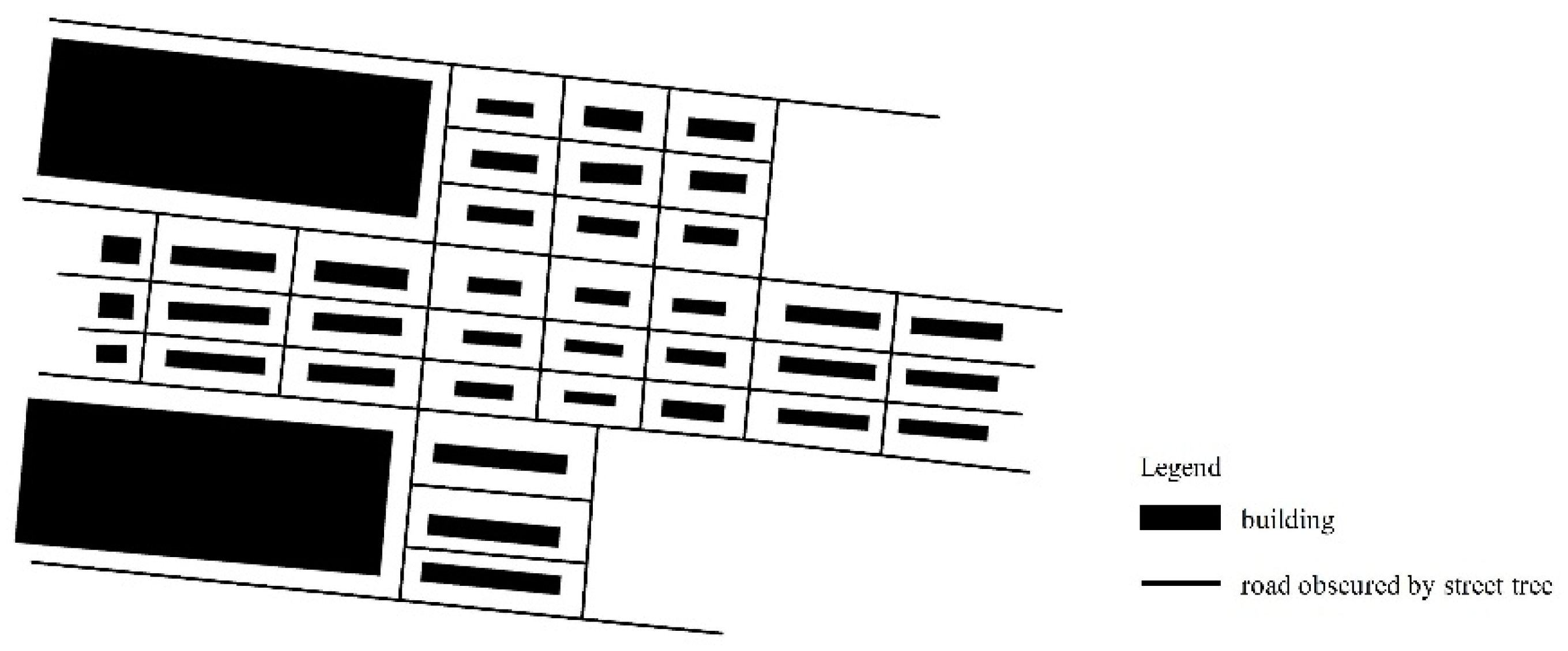
2.2.2. OpenStreetMap Road Network
- The road network is complete at a large scale; however, as the scale decreases, the completeness of the road network decreases, which means some roads totally disappear on low scales.
- Although some roads do not disappear, the road information is incomplete on a low scale.
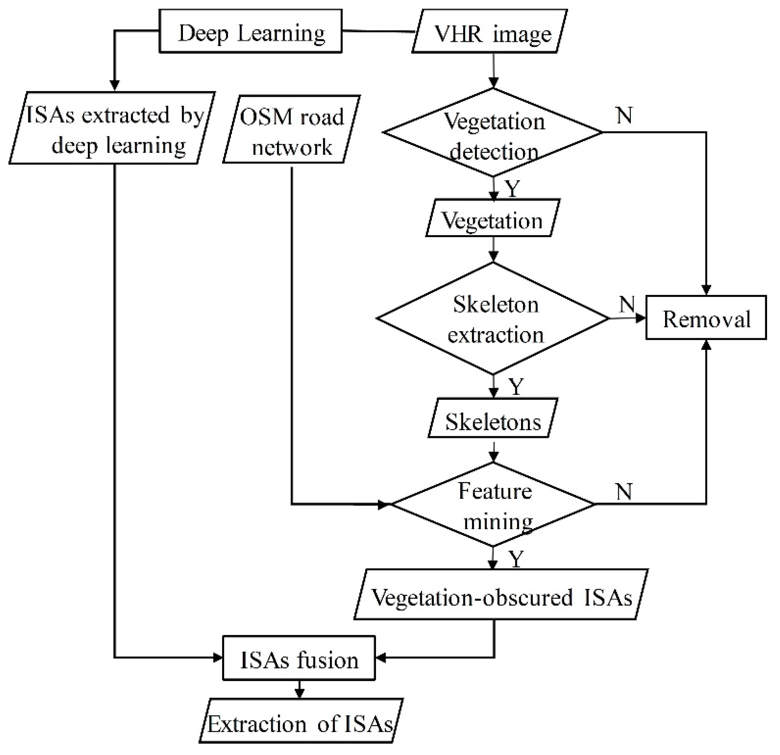
3. Methodology
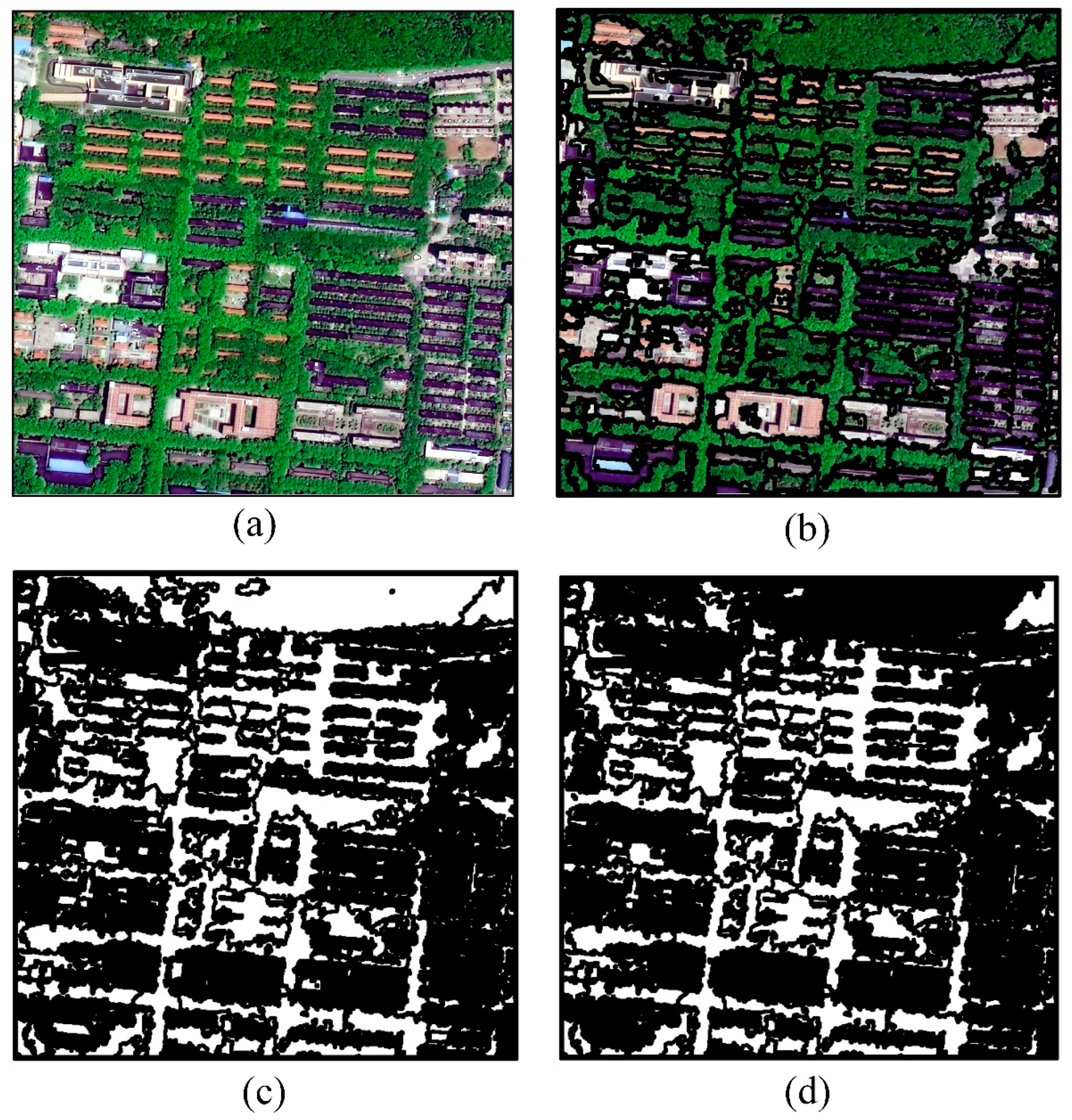
3.1. Vegetation Detection Based on Image Segmentation and Color VI
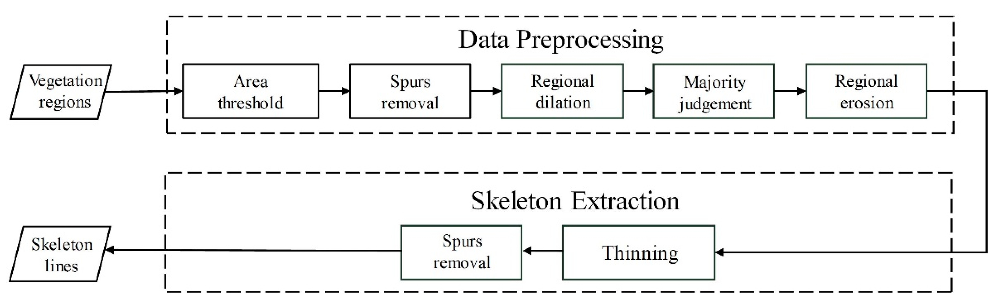
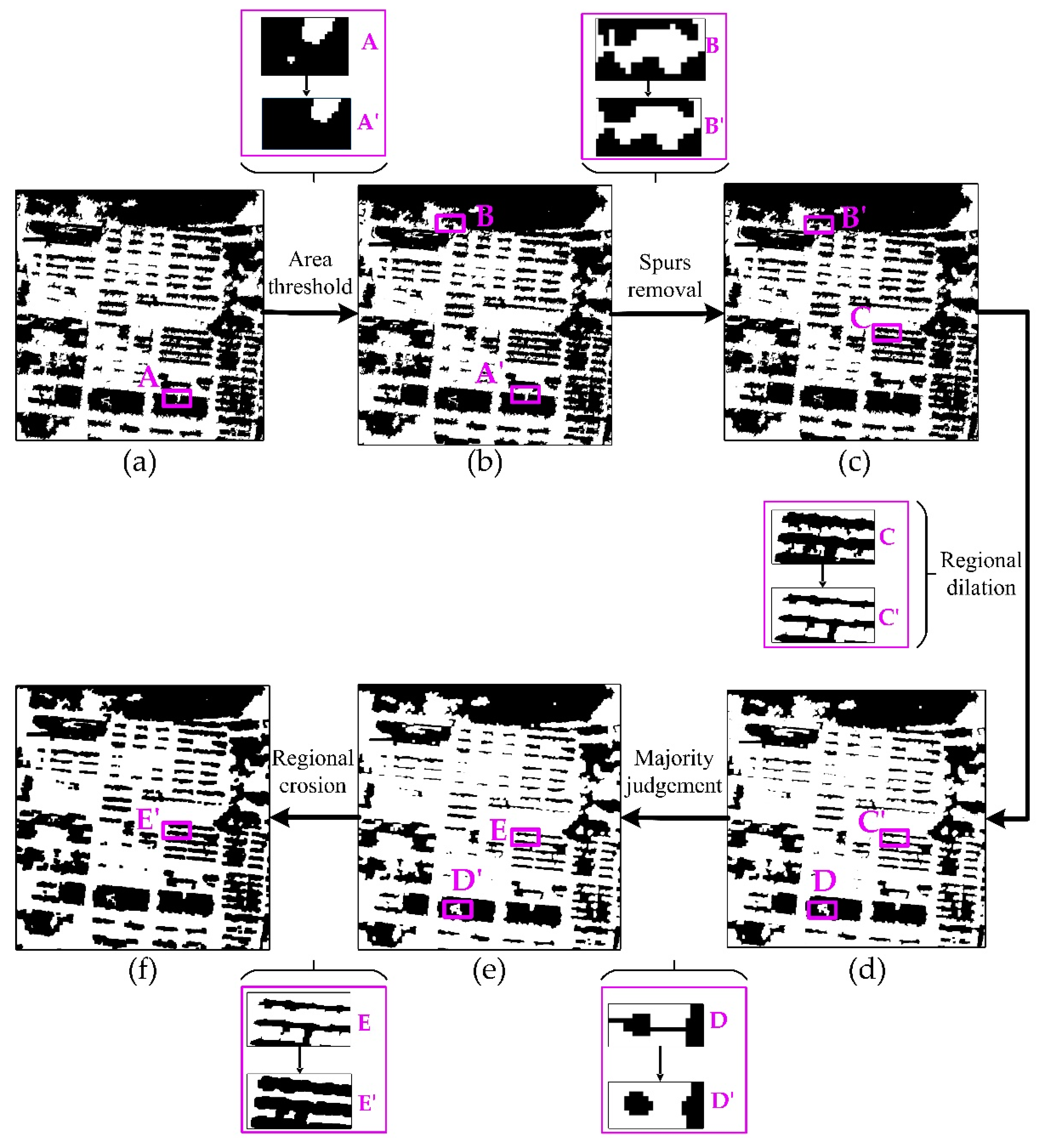
3.2. Skeleton Extraction
3.2.1. Data Preprocessing
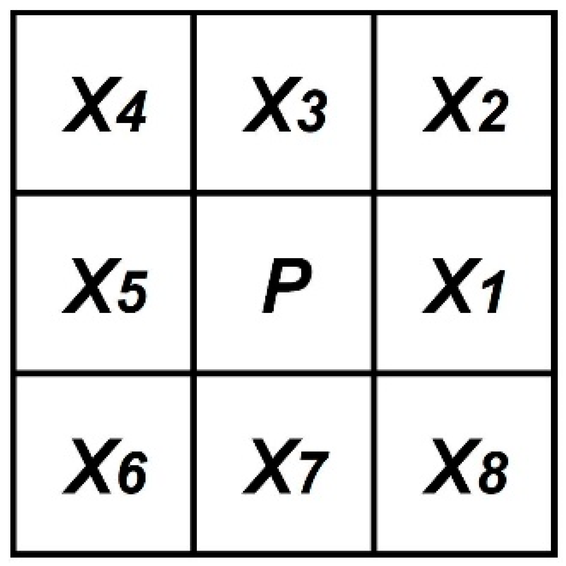
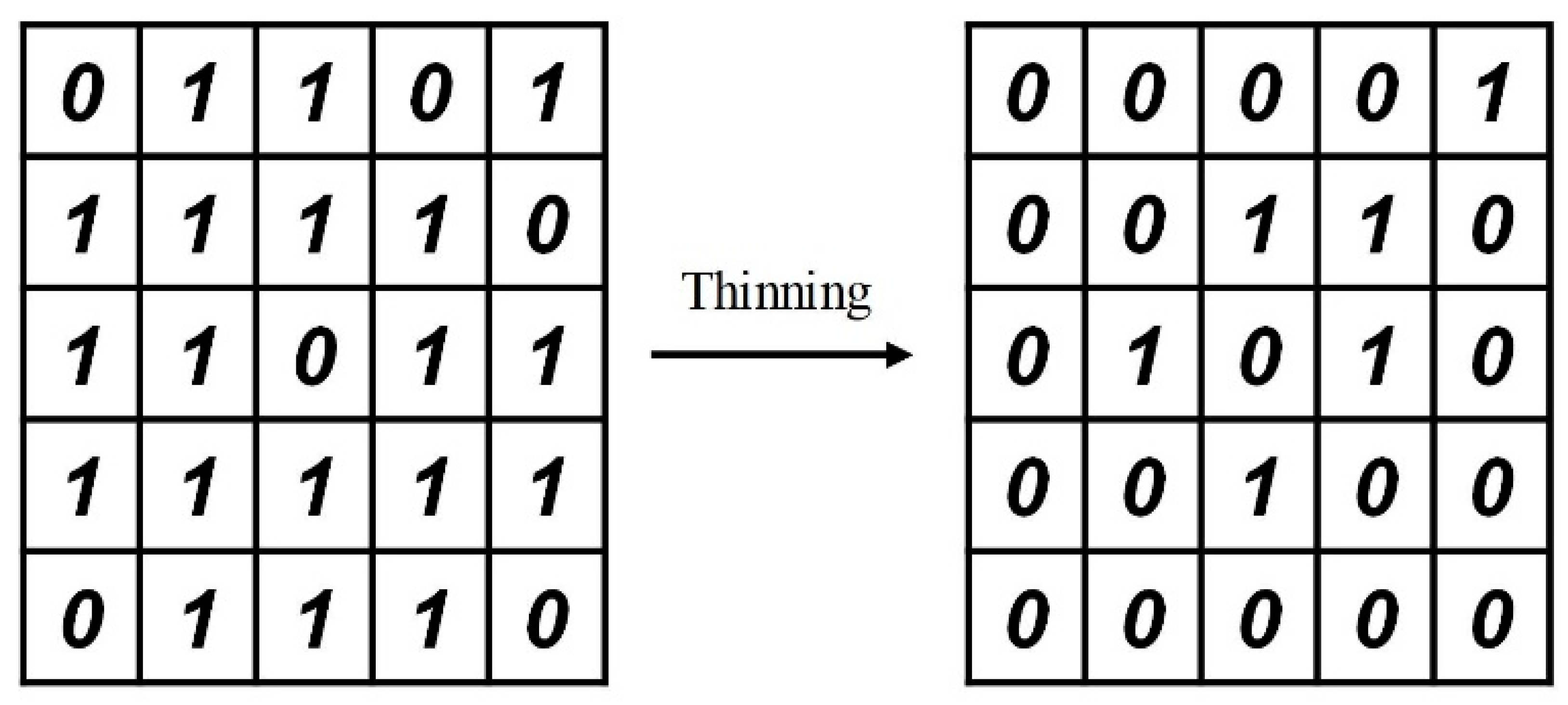
3.2.2. Skeleton Extraction
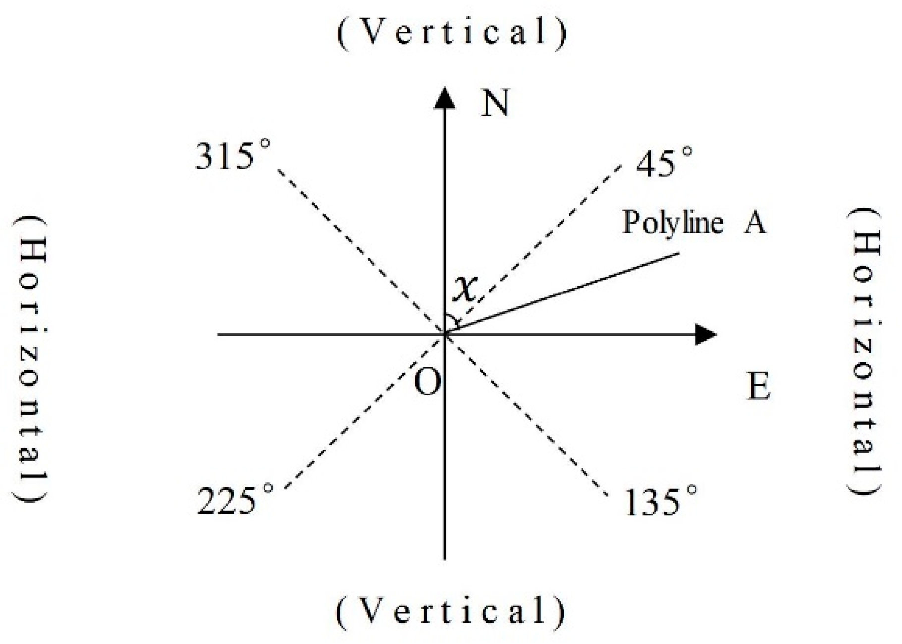
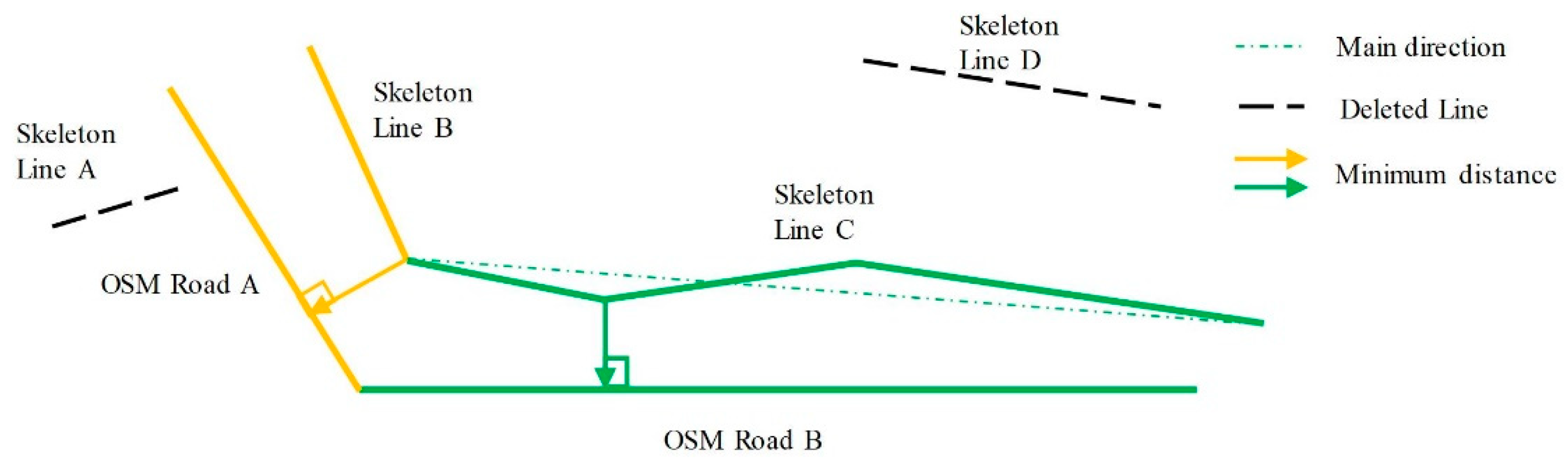
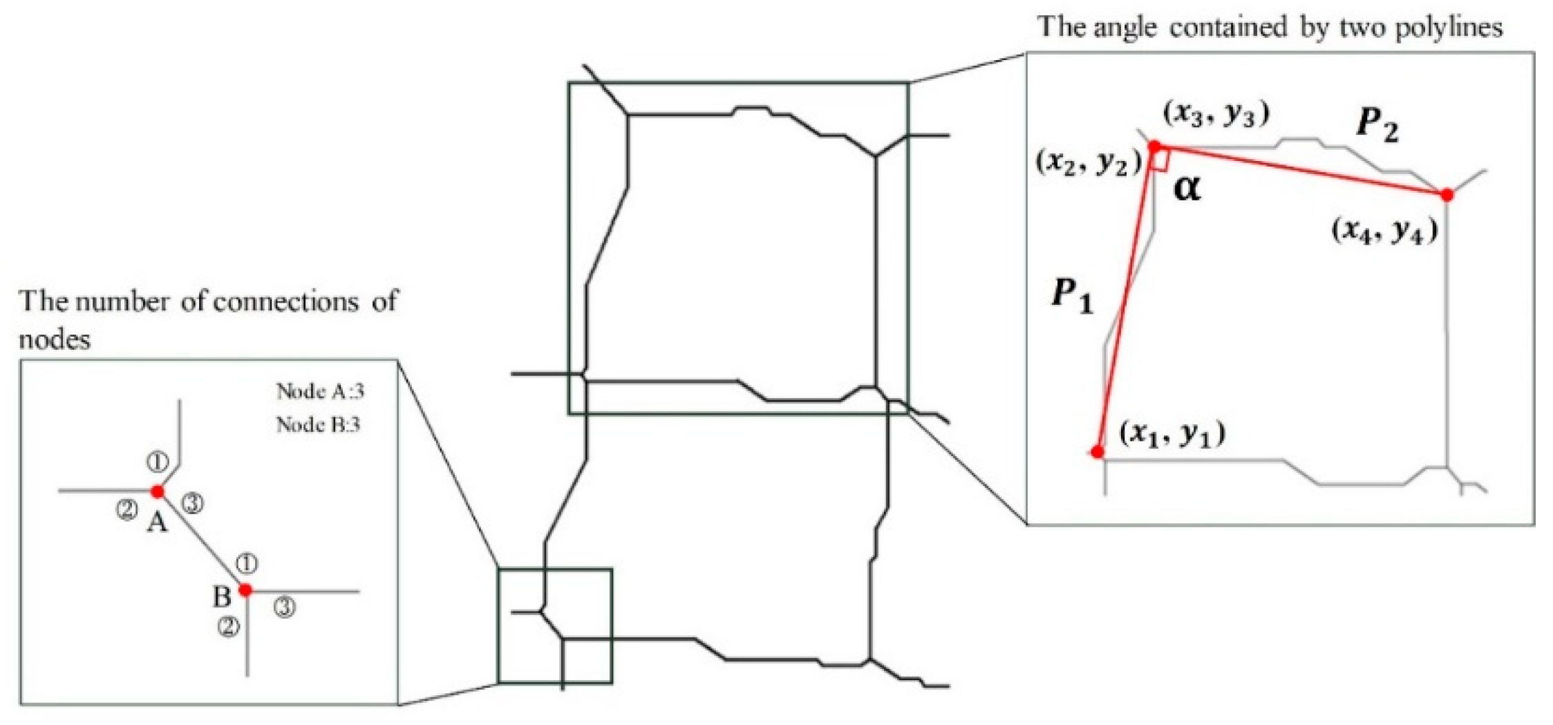
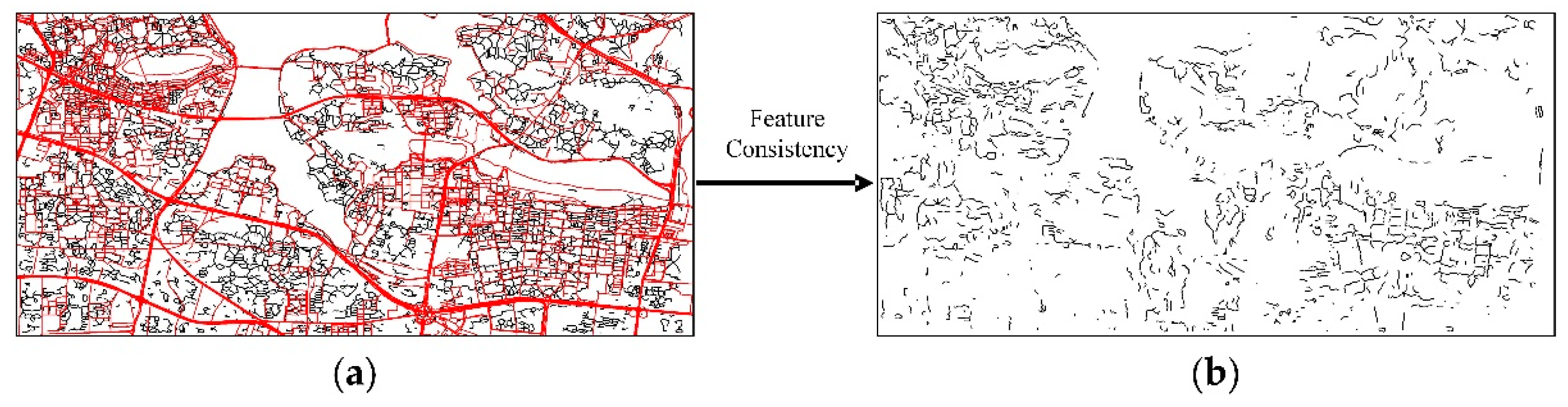
3.3. Feature Mining
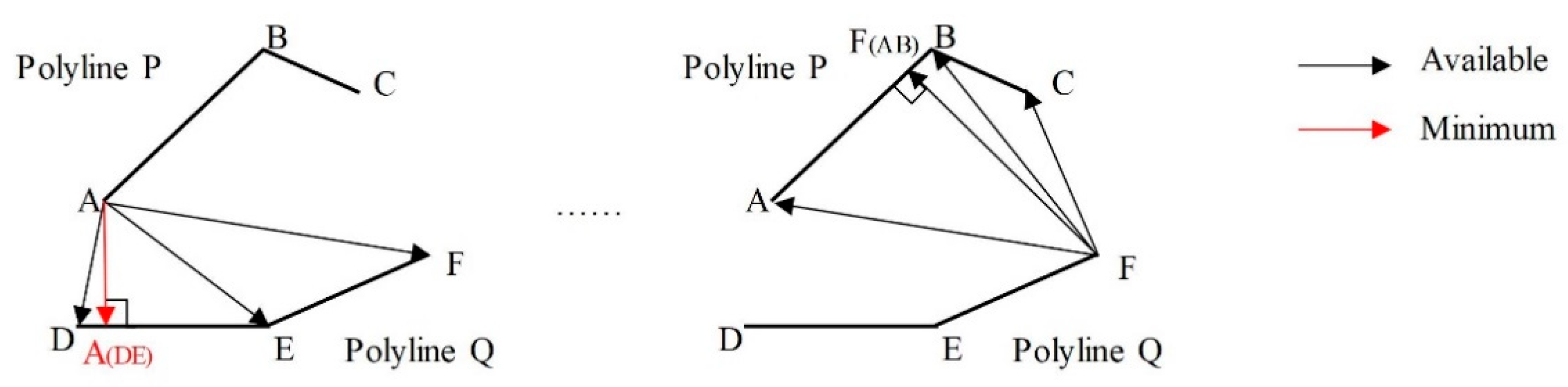
3.3.1. Feature Consistency
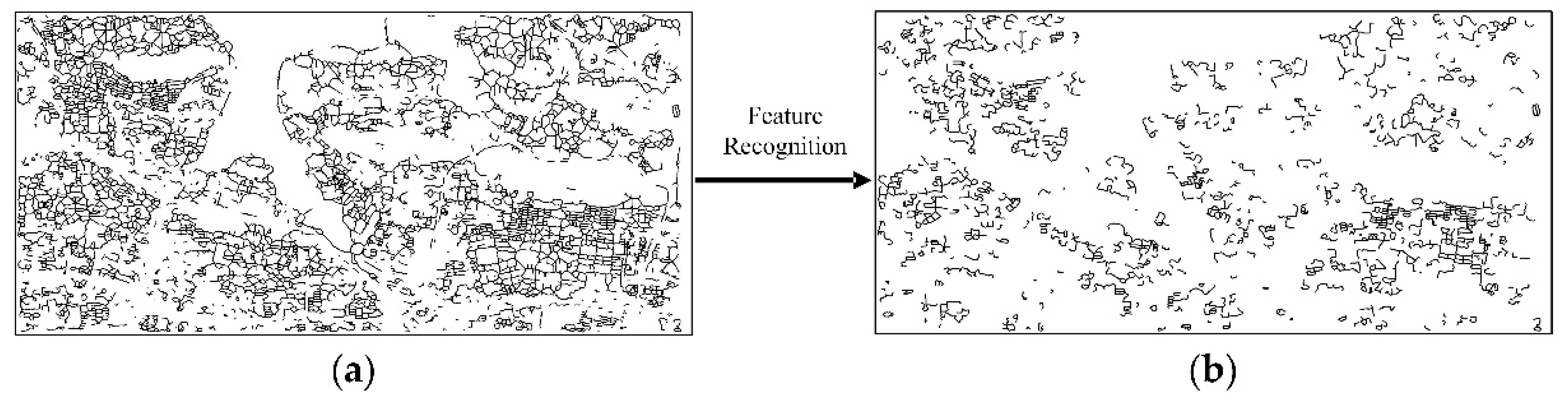
3.3.2. Feature Recognition
4. Results
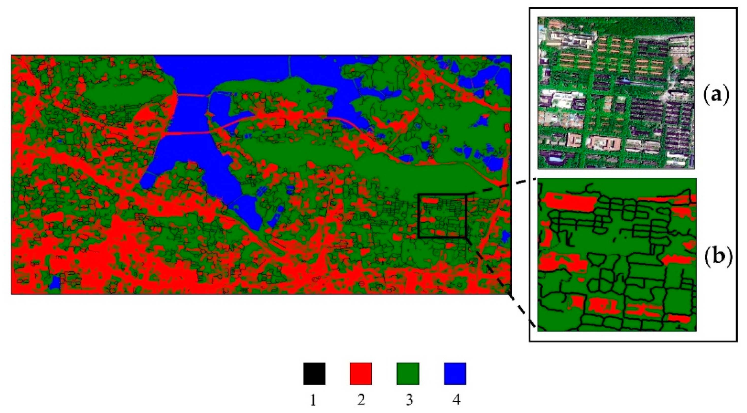
4.1. Vegetation Detection from the GF-2 Image
4.2. Skeleton Extraction Using Mathematical Morphology
4.3. Feature Mining
5. Discussion
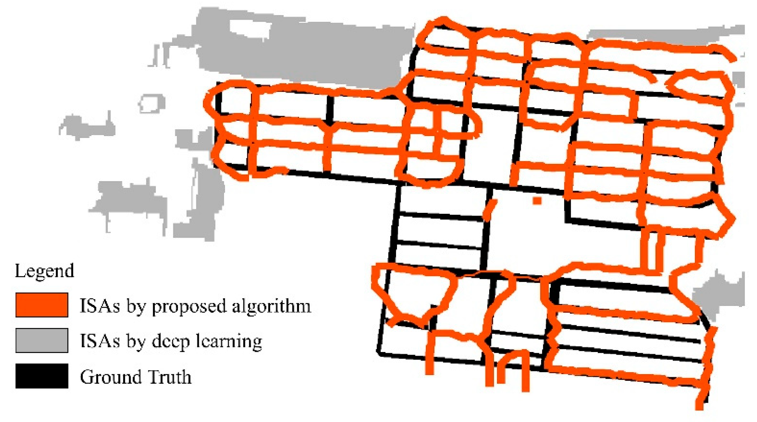
5.1. Deviation of Extracted Vegetation-Obscured ISAs
5.2. Network Structure of Extracted Vegetation-Obscured ISAs
5.3. Overestimation of Extracted Vegetation-Obscured ISAs
6. Conclusions
Author Contributions
Funding
Acknowledgments
Conflicts of Interest
References
- Shao, Z.; Fu, H.; Li, D.; Altan, O.; Cheng, T. Remote sensing monitoring of multi-scale watersheds impermeability for urban hydrological evaluation. Remote Sens. Environ. 2019, 232, 111338. [Google Scholar] [CrossRef]
- Coseo, P.; Larsen, L. Accurate Characterization of Land Cover in Urban Environments: Determining the Importance of Including Obscured Impervious Surfaces in Urban Heat Island Models. Atmosphere 2019, 10, 347. [Google Scholar] [CrossRef] [Green Version]
- Du, S.; Shi, P.; Van Rompaey, A.; Wen, J. Quantifying the impact of impervious surface location on flood peak discharge in urban areas. Nat. Hazards 2015, 76, 1457–1471. [Google Scholar] [CrossRef]
- Weng, Q. Remote sensing of impervious surfaces in the urban areas: Requirements, methods, and trends. Remote Sens. Environ. 2012, 117, 34–49. [Google Scholar] [CrossRef]
- Shao, Z.; Fu, H.; Fu, P.; Yin, L. Mapping Urban Impervious Surface by Fusing Optical and SAR Data at the Decision Level. Remote Sens. 2016, 8, 945. [Google Scholar] [CrossRef] [Green Version]
- Huang, F.; Yu, Y.; Feng, T. Automatic extraction of urban impervious surfaces based on deep learning and multi-source remote sensing data. J. Vis. Commun. Image Represent. 2019, 60, 16–27. [Google Scholar] [CrossRef]
- Parekh, J.R.; Poortinga, A.; Bhandari, B.; Mayer, T.; Saah, D.; Chishtie, F. Automatic Detection of Impervious Surfaces from Remotely Sensed Data Using Deep Learning. Remote Sens. 2021, 13, 3166. [Google Scholar] [CrossRef]
- Akbari, H.; Rose, L.S.; Taha, H. Analyzing the land cover of an urban environment using high-resolution orthophotos. Landsc. Urban Plan. 2003, 63, 1–14. [Google Scholar] [CrossRef]
- Gray, K.A.; Finster, M.E. The Urban Heat Island, Photochemical Smog and Chicago: Local Features of the Problem and Solution; Atmospheric Pollution Prevention Division, U.S. Environmental Protection Agency: Washington, DC, USA, 1999. [Google Scholar]
- Van der Linden, S.; Hostert, P. The influence of urban structures on impervious surface maps from airborne hyperspectral data. Remote Sens. Environ. 2009, 113, 2298–2305. [Google Scholar] [CrossRef]
- Weng, Q.; Lu, D. A sub-pixel analysis of urbanization effect on land surface temperature and its interplay with impervious surface and vegetation coverage in Indianapolis, United States. Int. J. Appl. Earth Obs. Geoinf. 2008, 10, 68–83. [Google Scholar] [CrossRef]
- Hu, X.; Weng, Q. Estimating impervious surfaces from medium spatial resolution imagery using the self-organizing map and multi-layer perceptron neural networks. Remote Sens. Environ. 2009, 113, 2089–2102. [Google Scholar] [CrossRef]
- Gong, C.; Wu, W. Comparisons of regression tree models for sub-pixel imperviousness estimation in a Gulf Coast city of Mississippi, USA. Int. J. Remote Sens. 2014, 35, 3722–3740. [Google Scholar] [CrossRef]
- Cai, C.; Li, P.; Jin, H. Extraction of Urban Impervious Surface Using Two-Season WorldView-2 Images: A Comparison. Photogramm. Eng. Remote Sens. 2016, 82, 335–349. [Google Scholar] [CrossRef]
- Hung, C.J.; James, L.A.; Hodgson, M.E. An Automated Algorithm for Mapping Building Impervious Areas from Airborne LiDAR Point-Cloud Data for Flood Hydrology. GIScience Remote Sens. 2018, 55, 793–816. [Google Scholar] [CrossRef]
- Zhang, J.; Li, P.; Mazher, A.; Liu, L. Impervious Surface Extraction with Very High Resolution Imagery In Urban Areas: Reducing Tree Obscuring Effect. In Proceedings of the Computer Vision in Remote Sensing (CVRS), Xiamen, China, 16–18 December 2012. [Google Scholar]
- Kaur, J.; Singh, J.; Sehra, S.S.; Rai, H.S. Systematic Literature Review of Data Quality within OpenStreetMap. In Proceedings of the International Conference on Next Generation Computing and Information Systems (ICNGCIS), Model Inst Engn & Technol, Jammu, India, 11–12 December 2017. [Google Scholar] [CrossRef]
- Li, P.; Guo, J.; Song, B.; Xiao, X. A Multilevel Hierarchical Image Segmentation Method for Urban Impervious Surface Mapping Using Very High-Resolution Imagery. IEEE J. Sel. Top. Appl. Earth Obs. Remote Sens. 2011, 4, 103–116. [Google Scholar] [CrossRef]
- Jin, X. Segmentation-Based Image Processing System. U.S. US8260048 B2, 9 April 2012. [Google Scholar]
- Roerdink, J.B.T.M.; Meijster, A. The Watershed Transform: Definitions, Algorithms, and Parallelization Strategies. Fundam. Inform. 2000, 41, 187–228. [Google Scholar] [CrossRef] [Green Version]
- Robinson, D.J.; Redding, N.J.; Crisp, D.J. Implementation of a Fast Algorithm for Segmenting Sar Imagery. In Proceedings of the Scientific and Technical Report, Australia: Defense Science and Technology Organization, 1 January 2002. [Google Scholar]
- Luo, Y.; Xu, J.; Yue, W. Research on vegetation indices based on remote sensing images. Ecol. Sci. 2005, 24, 75–79. [Google Scholar]
- Woebbecke, D.M.; Meyer, G.E.; Vonbargen, K.; Mortensen, D.A. Color Indices for Weed Identification under Various Soil, Residue and Lighting Conditions. Trans. ASAE 1995, 38, 259–269. [Google Scholar] [CrossRef]
- Meyer, G.E.; Neto, J.C. Verification of Color Vegetation Indices for Automated Crop Imaging Applications. Comput. Electron. Agric. 2008, 63, 282–293. [Google Scholar] [CrossRef]
- Ma, H.; Cheng, X.; Wang, X.; Yuan, J. Road Information Extraction from High-Resolution Remote Sensing Images Based on Threshold Segmentation and Mathematical Morphology. In Proceedings of the 6th International Congress on Image and Signal Processing (CISP), Hangzhou, China, 16–18 December 2013. [Google Scholar]
- Zhou, H.; Song, X.; Liu, G. Automatic Road Extraction from High Resolution Remote Sensing Image by Means of Topological Derivative and Mathematical Morphology. In Proceedings of the Remote Sensing Image Processing and Geographic Information Systems. 10th International Symposium on Multispectral Image Processing and Pattern Recognition (MIPPR)—Remote Sensing Image Processing, Geographic Information Systems, and Other Applications, Xiangyang, China, 28–29 October 2017. [Google Scholar] [CrossRef]
- Lam, L.; Lee, S.W.; Suen, C.Y. Thinning methodologies—A comprehensive survey. IEEE Trans. Pattern Anal. Mach. Intell. 1992, 14, 869–885. [Google Scholar] [CrossRef] [Green Version]
- Cai, B.; Wang, S.; Wang, L.; Shao, Z. Extraction of Urban Impervious Surface from High-Resolution Remote Sensing Imagery Based on Deep Learning. J. Geo-Inf. Sci. 2019, 21, 1420–1429. [Google Scholar]
- Shao, Z.; Cheng, G.; Li, D.; Huang, X.; Lu, Z.; Liu, J. Spatiotemporal-Spectral-Angular Observation Model that Integrates Observations from UAV and Mobile Mapping Vehicle for Better Urban Mapping. Geo-Spat. Inf. Sci. 2021, 24, 615–629. [Google Scholar] [CrossRef]
- Shao, Z.; Wu, W.; Li, D. Spatio-temporal-spectral observation model for urban remote sensing. Geo-Spat. Inf. Sci. 2021, 24, 372–386. [Google Scholar] [CrossRef]


| Satellite Name | Spatial Resolution (m) | Number of Bands | Coordinate System | Range of Study Area | Acquisition Season |
|---|---|---|---|---|---|
| GF-2 | 0.8 | 3 (Red, Green, Blue) | WGS84 | 30.50–30.54° N 114.35–114.42° E | Summer, 2020 |
| Num | Field Name | Description | Buffer Width (m) |
|---|---|---|---|
| 1 | Motorway | Mainly high-grade roads, on which vegetation usually covers the road shoulders or non-motorized lanes attached to high-grade roads. The coverage of vegetation is not broad. | 1.25 |
| 2 | Trunk | ||
| 3 | Secondary | ||
| 4 | Tertiary | ||
| 5 | Trunk_link | ||
| 6 | Secondary_link | ||
| 7 | Cycleway | ||
| 8 | Unclassified | Contains some special road types. It should be noted that “Unclassified” does not mean that the classification is unknown. It refers to the least important roads in a country’s system. | 4.5 |
| 9 | Residential | ||
| 10 | Living_street | ||
| 11 | Service | ||
| 12 | Null | Roads without grade | |
| 13 | Pedestrian | Only for people to walk. | 1 |
| 14 | Footway | ||
| 15 | Steps | ||
| 16 | Path | A non-specific path. It can be used as a cycleway or sidewalk. | |
| 17 | Construction | Roads under construction, do not study | 0 |
| Proposed Algorithm | |
|---|---|
| PA | 79.98% |
| UA | 56.08% |
| OA | 86.64% |
Publisher’s Note: MDPI stays neutral with regard to jurisdictional claims in published maps and institutional affiliations. |
© 2022 by the authors. Licensee MDPI, Basel, Switzerland. This article is an open access article distributed under the terms and conditions of the Creative Commons Attribution (CC BY) license (https://creativecommons.org/licenses/by/4.0/).
Share and Cite
Mao, T.; Fan, Y.; Zhi, S.; Tang, J. A Morphological Feature-Oriented Algorithm for Extracting Impervious Surface Areas Obscured by Vegetation in Collaboration with OSM Road Networks in Urban Areas. Remote Sens. 2022, 14, 2493. https://0-doi-org.brum.beds.ac.uk/10.3390/rs14102493
Mao T, Fan Y, Zhi S, Tang J. A Morphological Feature-Oriented Algorithm for Extracting Impervious Surface Areas Obscured by Vegetation in Collaboration with OSM Road Networks in Urban Areas. Remote Sensing. 2022; 14(10):2493. https://0-doi-org.brum.beds.ac.uk/10.3390/rs14102493
Chicago/Turabian StyleMao, Taomin, Yewen Fan, Shuang Zhi, and Jinshan Tang. 2022. "A Morphological Feature-Oriented Algorithm for Extracting Impervious Surface Areas Obscured by Vegetation in Collaboration with OSM Road Networks in Urban Areas" Remote Sensing 14, no. 10: 2493. https://0-doi-org.brum.beds.ac.uk/10.3390/rs14102493