1. Introduction
Image registration [
1,
2] is one of the most basic and challenging tasks in remote sense image processing. Its main goal is to geometrically align two images of the same, or similar scene [
3] from different perspectives, different moments, and even different imaging methods. It is an essential prerequisite for the analysis and for processing two or more images. Image registration is widely used in many remote sensing fields, such as image-stitching, image fusion, change detection, and environmental monitoring [
4,
5,
6,
7,
8].
Image registration methods can be roughly divided into two categories, one is region-based methods and the other is feature-based methods. Region-based methods establish matching correspondences by pixel intensities in the intersection of two images with a certain similarity, and such methods usually do not detect features. Feature-based methods extract feature points and descriptors from images and then establish matching correspondences based on their similarity or geometric relationship constraints [
3]. These methods need to detect features.
Feature-based methods are more robust when dealing with remote-sensing images with image distortion, significant illumination changes, and significant noise effects. In this paper, we focus on feature-based image registration methods. We transform the problem of image registration into the problem of matching between discrete feature points in two images.
These discrete feature points are obtained by general-purpose feature detectors, such as scale-invariant feature transform (SIFT) [
9], speeded up robust features (SURF) [
10], oriented FAST and rotated BRIEF (ORB) [
11], etc. In the feature-matching processes, it is often necessary to compare the feature points in the two images one by one so that the matching space of all possible matches is large. Assuming that there are
N feature points to be matched in the two images, a total of
arrangements [
12] need to be computed, which is inevitably time-consuming.
To overcome this challenge, researchers filter out untrusted outliers through similarity constraints, thereby obtaining a initial set of putative correspondences containing only similar descriptors. Then, our method only needs to judge the correctness of the initial matching correspondences in the hypothetical set, to remove the false matching, and to establish an accurate correspondence. This method greatly reduces the amount of computation.
Researchers have designed a variety of algorithms to achieve the problem of removing false matching [
13,
14,
15]. However, it is still a challenging and urgent task to design a general and efficient matching algorithm to handle various feature matching problems in real scenes when faced with the registration problem of remote-sensing images. Remote-sensing images mainly have the following characteristics: First, remote-sensing images are mostly pictures of cities, mountains, farmland, and other complex scenes taken by an unmanned aerial vehicle (UAV) in the air.
Secondly, remote-sensing images have many great challenges that affect image registration, such as a large field of view, low image quality, serious geometric distortion and obvious viewpoint changes. Researchers proposed a series of methods based on the consistency of neighborhood topology to solve the above problems. For example, Ma et al. [
16] proposed a Locality Preserving Matching (LPM) method. By observing the differences between image pairs of various transformation types, with LPM, they found that, although the Euclidean distance between the feature points of the image pairs changes, the topological structure of the feature points and their neighboring points does not change easily, in realizing remote-sensing image matching using this property.
However, methods based on neighborhood topology consistency fail in the following two cases: (1) Some false matches and their neighborhood point pairs can also remain similar in relative directions and lengths. (2) Some correct matches cannot maintain the relative orientation consistency of neighborhood topology when there are severe geometric distortions and obvious viewpoint changes between image pairs. Therefore, using only neighborhood topology consistency cannot solve the above problems well.
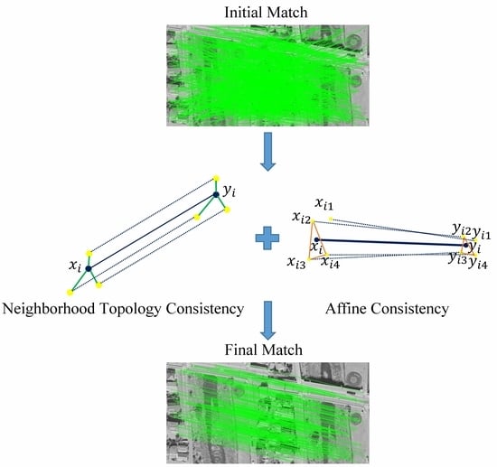
In order to solve the above problems, in this paper, we propose a method that combines neighborhood topological consistency with affine constraints for the feature matching of remote-sensing images. We found that affine consistency is a more general feature within a small local area of image, and the general affine transformation [
17] can well model the topology of the internal small local region of the image. Thus, further introducing affine consistency between matching points and their neighboring point pairs can be well applied to the above two cases. The proposed method is more general and can handle remote-sensing image pairs with multiple transformation types by preserving topological consistency and affine constraints among neighborhood matches.
Our method has the following two contributions: (1) We introduce local affine constraints into the neighborhood topology consistency approach. This method can deal with the problems of severe geometric distortion and obvious viewpoint change of images that can not be overcome by previous methods. (2) We formulate the problem as a mathematical model, derive its solution, and then conduct qualitative, quantitative, and robust experiments on four remote-sensing-image datasets. Experimental results show that our method has better matching performance than other mainstream methods and can deal with matching problems in milliseconds.
The organization of this article is as follows. Related work and background are presented in
Section 2.
Section 3 proposes a strongly constrained remote-sensing image registration method based on preserving neighborhood topological consistency and an affine transformation model constraints. Then, in
Section 4, we present our qualitative, quantitative, and robust experimental results on four different types of remote-sensing-image datasets. Finally,
Section 5 summarizes the full text.
2. Related Works
Image registration is widely used in computer vision [
18,
19], pattern recognition [
20,
21,
22], medical imaging [
23,
24], and especially remote-sensing image analysis [
25,
26,
27,
28]. From some literature reviews, we can find a detailed introduction on image registration methods [
3,
29]. In the past few decades, image registration technology has developed rapidly, and many methods for image matching have been proposed. These methods are roughly divided into region-based methods and feature-based methods. The region-based method does not detect image features but directly processes the image pixel level.
For example, Zhou et al. [
30] proposed a cross-weather road scene registration method based on a latent generative model of intensity constancy, which is a dense matching method. It contains three types of methods: correlation-like methods [
31], Fourier methods [
32], and mutual information methods [
33]. This kind of method can show better effect when there are less detailed features in the image. However, feature-based methods can show better results when we deal with remote-sensing images with significant detailed texture features. It is worth mentioning that these methods will be more popular due to their lower complexity when the image has unfavorable factors, such as low quality, shadows, noise, obvious viewpoint changes, and geometric distortions.
We pay more attention to the feature-based matching methods. We mean to establish the correct corresponding relationship of pixels or points between two images by extracting image feature points and their descriptors. Then, the spatial transformations are estimated based on the results, which can be used to align a given pair of images. We also call this process feature matching, where the main purpose is to establish a one-to-one correspondence between feature point sets of image pairs. It can be divided into indirect matching and direct matching according to whether the local descriptor is used.
Direct matching is to directly use spatial geometric relations and optimization methods to establish correspondences from two given feature sets. Loiola et al. [
34] proposed a direct matching method based on secondary assignment. Sofka et al. [
35] studied the modeling of uncertainty in the registration process and proposed a covariance-driven correspondence method in an em-like framework. Indirect matching establishes the correct correspondences by establishing the correspondences between the similarity of the descriptors and the distance judged from the measurement space and then removing false matches.
Some parametric model-based methods, such as Maier et al. [
36] introduced a statistical optical flow-based guided matching method, RANSAC and its variants MLESAC [
37] and PROSAC [
38]. These methods have been widely used in image registration in the remote-sensing field. However, when there are many outliers and non-rigid transformations occur, these methods are no longer applicable.
To establish a robust feature-point correspondence between remote-sensing image pairs, we follow a two-step strategy [
39,
40]: (1) calculate an initial set of hypothetical correspondences and (2) according to the geometric constraints between point pairs, the outliers in the hypothetical set are removed to establish an accurate correspondence. In the first step, researchers have proposed a variety of classic and widely used feature matching algorithms to establish correspondences.
For example, Lowe [
9] proposed a SIFT algorithm, the essence of which is to find key points in different scale spaces and calculate the direction of the key points. Then, by comparing the feature vectors of each key point pairwise, several pairs of feature points that match each other are found, and the corresponding relationship between the image pairs is established. Rublee et al. [
11] proposed the ORB algorithm, which uses the FAST algorithm to detect feature points, then uses the BRIEF algorithm to calculate the descriptor of a feature point, and finally obtains the corresponding relationship according to the preset threshold and the similarity of the descriptors.
In order to achieve the removal of outliers in the hypothetical set in the second-step strategy, researchers have proposed a number of methods. In remote-sensing image registration, Ma et al. [
41] proposed a guided locality-preserving matching method for the robust feature matching of remote-sensing images. Wu et al. [
42] proposed an estimation method based on weighted total least squares (WTLS) and introduced it into remote-sensing image registration, which can obtain more robust model parameter estimation and higher registration precision.
Ma et al. [
43] proposed a robust remote-sensing image feature matching algorithm based on Lq estimation, which achieved better results. In addition, some nonparametric interpolation methods have been proposed [
44], especially in remote-sensing image registration. These methods insert prior knowledge conditions into nonparametric functions, and they apply to a motion field with slow and smooth correspondences.
However, these methods have high computational complexity, and the high time-consumption affects their application in real-time tasks. LPM [
16] further preserves the distribution of transformed neighborhood point pairs on the constraint that the distances between general feature correspondences are preserved. At the same time, considering the topology constraints of adjacent elements, LPM transforms the hypothetical matching into displacement vectors, where the head and tail of each vector correspond to the spatial positions of the two corresponding feature points in the two images, and defines the neighborhood topology consistency based on the length ratio and included angle of the vectors to achieve the elimination of mismatching.
Zhou et al. [
45] proposed a non-rigid feature matching method for remote-sensing images through probabilistic inference with global and local regularization. These methods focus on the constraints of the neighborhood structure, which is a great inspiration for our method.
3. Methods
This section describes a method for establishing precise correspondences between feature points extracted from two identical or similar images. This method follows a two-step strategy. First, we need to construct a hypothetical set of matching point pairs. Fortunately, more mature feature matching algorithms, such as SIFT and ORB can help us to initially filter out the clearly different matching point pairs between the two feature point sets and to find all the initial matching point pairs that are sufficiently trusted.
Thus, the first step strategy is easy to complete. The focus of our research is the second step strategy. We use a well-designed geometric relationship to constrain the matching correspondences in the hypothetical matching set, and eliminate those mismatched point pairs that do not retain the spatial neighborhood structure and the local affine transformation constraints. Below, we discuss in detail how to eliminate false matches in the second step.
3.1. Problem Formulation
Suppose there is a set of N hypothetical feature-point correspondences extracted from two given identical or similar images, where and , respectively, represent the two-dimensional vectors coordinates of the feature points extracted from the two images using the SIFT algorithm. The corresponding relationship of the i-th hypothetical feature point is represented by . Our goal is to eliminate the mismatched point pairs in the hypothetical set S and construct accurate feature-point correspondences accordingly.
If, an image pair has only undergone rigid transformation, then the distances between all feature correspondences will be preserved. We use
to represent the unknown inlier point set [
16], and its optimal solution can be expressed as follows:
where the cost function is denoted by
C and defined as:
In Equation (
2),
d represents the Euclidean distance between two feature points, and
denotes the cardinality of a set. In this cost function, the first term penalizes any match which does not preserve the distance of a point pair, and the second term prevents outliers [
16]. We set the parameter
to balance these two items. In the case of an ideal rigid transformation, the optimal solution should reach zero penalty, which means that the first term of the cost function
C should be zero.
However, simple rigid transformations are rare in reality. The distance relationship between the above-mentioned feature point pairs cannot be well preserved when a given pair of two images undergoes a complex non-rigid transformation, especially for those matching point pairs with a longer distance. Even though there is a clear viewpoint change and non-rigid deformation between the two images due to the physical constraints between the regions around the feature points, the local neighborhood structure between the transformed feature point pairs can be well preserved. Therefore, by preserving only local structures, the cost function in Equation (
2) becomes:
The feature point set does not have a clear neighborhood definition. Therefore, we independently defined a simple neighborhood representation method, which is to search for the
K leading points with the closest Euclidean distance for each point in the feature point set. In Equation (
3),
denotes the neighborhood of feature point
, and
is the normalization factor for processing the first term.
In the case of non-rigid transformation, the absolute distance
d of the feature point pair cannot be maintained well. In order to facilitate subsequent calculations, LPM quantizes the distance metric
d into two levels as:
3.2. Consistency of Neighborhood Structure
The above Equation (
3) eliminates mismatches by minimizing the cost function
C. This process essentially only preserves the distance relationship of the local structure without considering the constraints of the topological structure between the neighborhood of the feature point pairs. The performance of eliminating mismatches is greatly degraded when encountering complex scenes where two images have many similar patterns as shown in
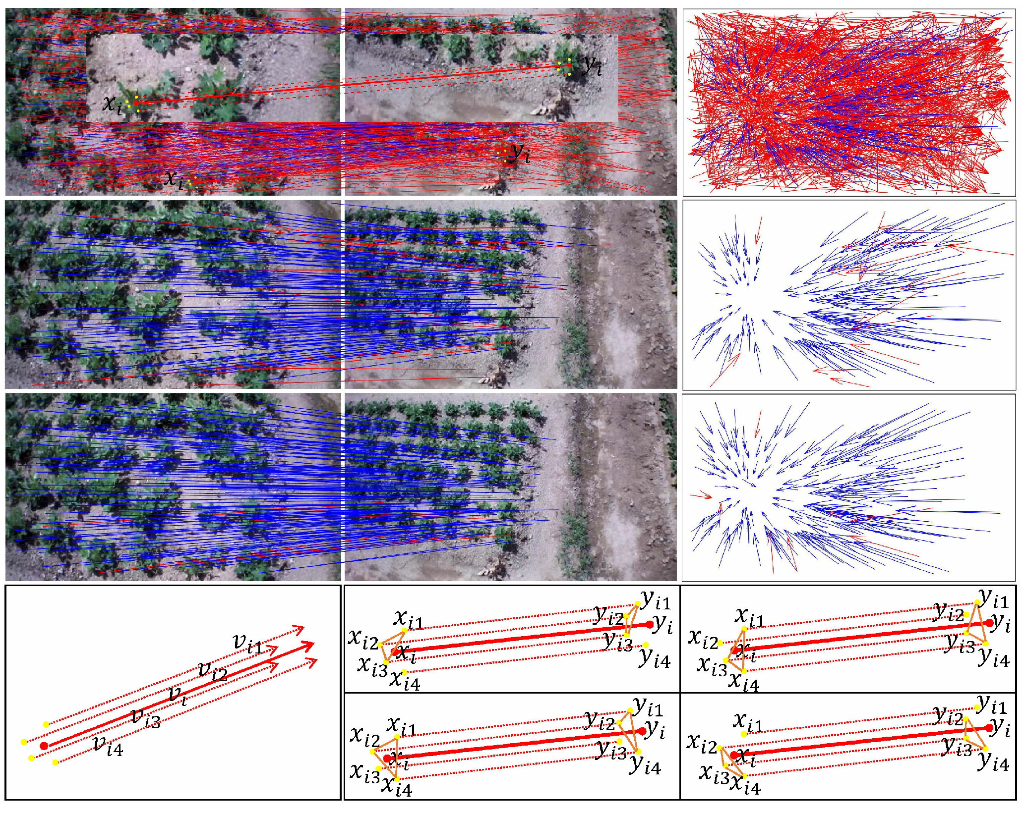
Figure 1. Therefore, we strengthen the constraints of the topological structure to improve its ability to eliminate mismatches.
As shown in
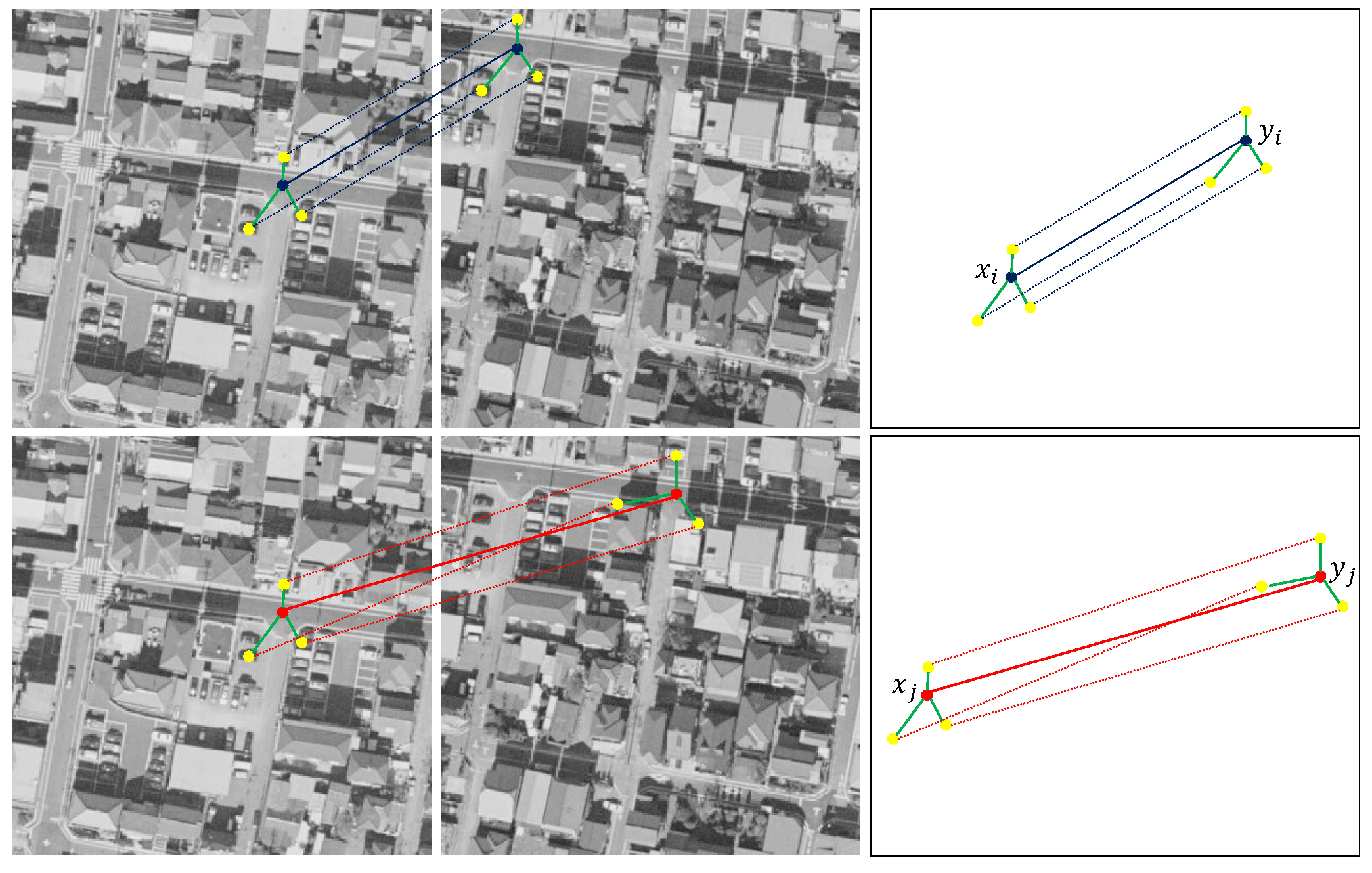
Figure 1, we use
and
to represent a feature point of two given images, and
is a pair of feature correspondence in the hypothetical set
S. The above part represents a pair of correct matching points, which are also called inliers and connects them with a blue line, where its neighborhood points are connected by blue dotted lines. The below part represents a pair of false matching points, also called outliers connected with red lines, and its neighborhood points are connected by red dotted lines.
For each feature point and , we search for the three leading points with the closest Euclidean distance as the neighborhood of feature points according to the mentioned definition of the previous neighborhood. We use green lines to connect the feature points and their neighborhood points to represent the topological structure of the feature point neighborhood. We can clearly see the huge difference in the topological structure of the above and below parts.
For the correct matching point pairs in the above part, the topological structures of the respective neighborhood of and are almost the same, and the direction and distance of the neighborhood points are almost the same; the false matching point pairs in the below part are the opposite. It is precisely by taking advantage of this obvious difference that we have designed an algorithm that uses the constraints of the neighborhood topology to eliminate mismatches.
One of the properties of similar triangles is that the corresponding angles are equal and the ratio of the lengths of the corresponding sides is proportional. It is proposed in LRO [
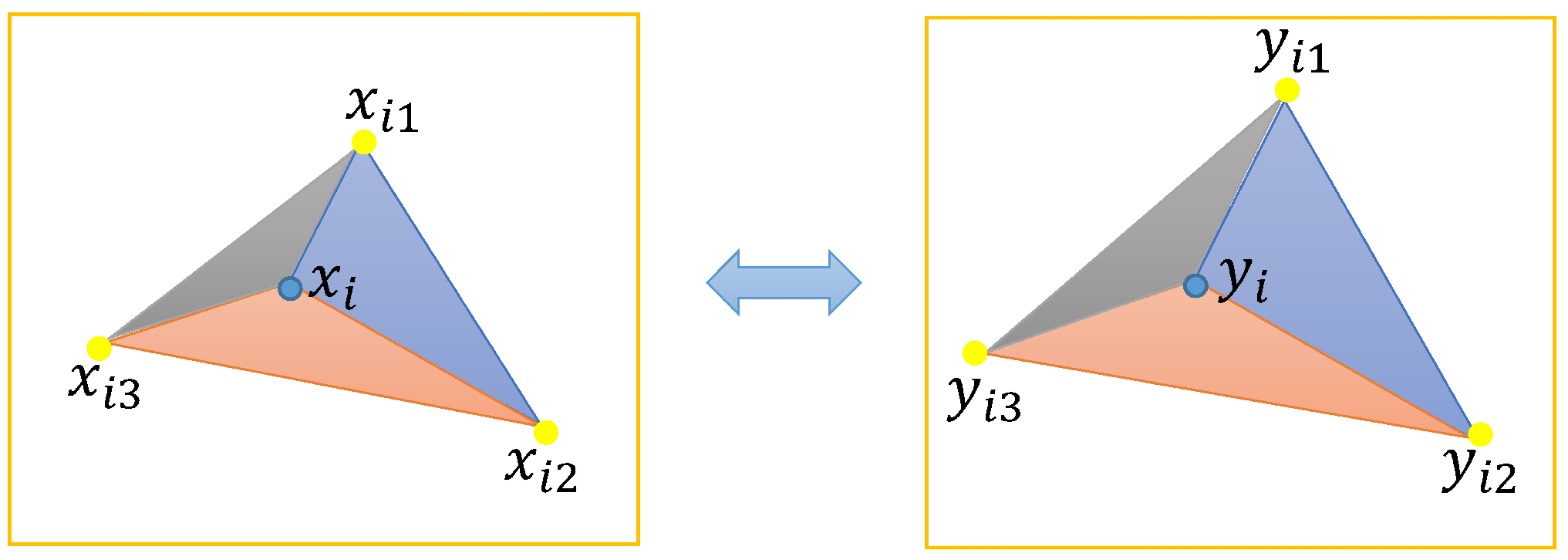
46] that, although the absolute coordinates of a pair of correct matching points are different in their respective images, the angle formed between the feature points and their neighborhood points should remain the same. Unlike LRO, we add a further geometric constraint, which is that the ratio of lengths between neighborhood points should remain the same.
As shown in
Figure 2, we extend the properties of similar triangles to triangles composed of feature points and any two adjacent neighborhood points, and construct a local neighborhood similar triangle of matching point pairs. Given the feature point
and its neighborhood points
,
,
, they can form three triangles:
,
, and
. Correspondingly, given the feature point
and its neighborhood points
,
,
, they can form three triangles:
,
, and
. From this, we can obtain the following expression:
3.3. Affine Transformation Model
The consistency of the topological structure of the neighborhood around the matching points cannot be maintained well when the given two images have severe geometric distortions and the viewpoints within the images change greatly. The transformation model refers to the selected geometric transformation model that can best fit the changes between the two images in the case of geometric distortion between the image to be matched and the background image.
Due to the large number of outliers in the initial hypothetical set S, we cannot establish a global and accurate transformation model for this transformation. However, the topological structure of the local area in the image can still be kept consistent with an affine transformation model.
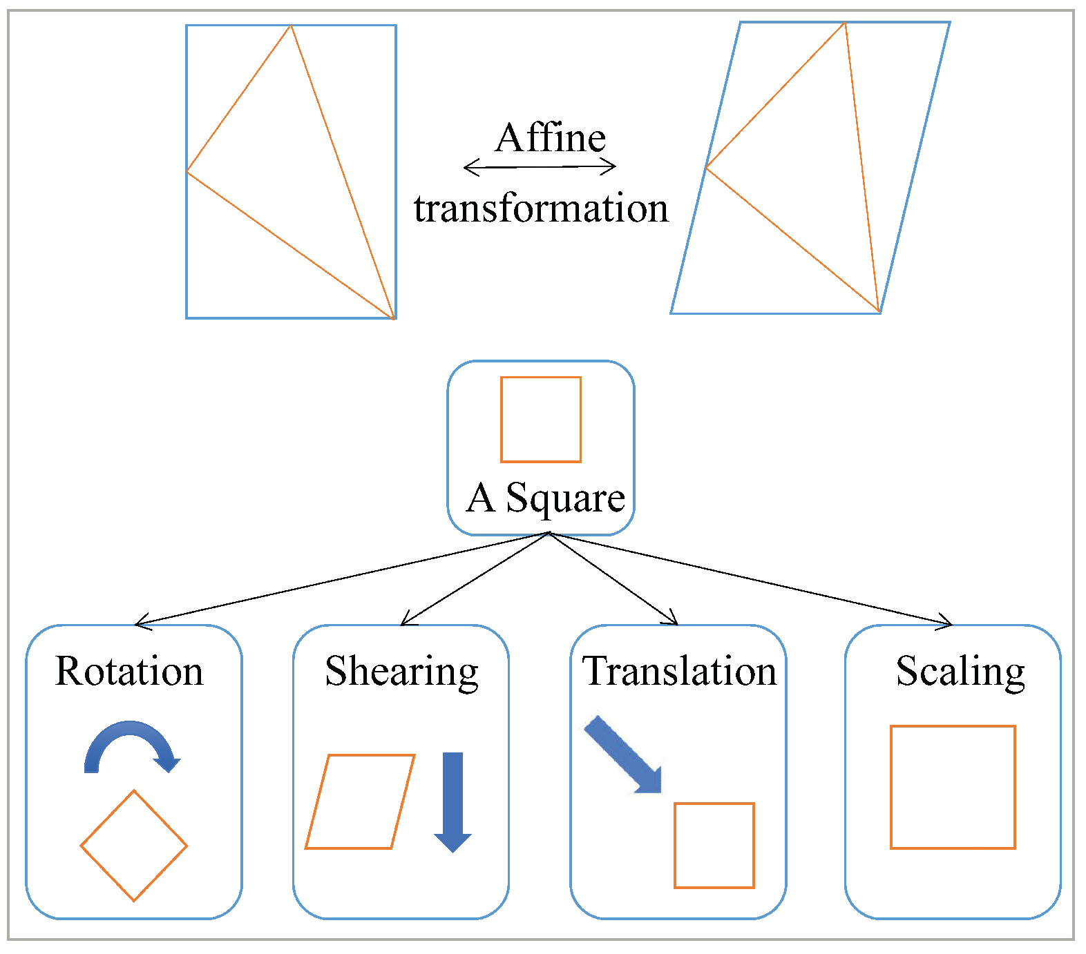
As shown in
Figure 3, affine transformation is a linear transformation from 2D-to-2D coordinate, which can maintain the straightness and parallelness of images transformed by translation, scaling, inversion, rotation and shearing, that is, keep the relative position relationship between 2D images unchanged. Equation (
7) expresses the formula of affine transformation, where
represents the amount of translation, and the parameter
reflects the transformation of the image, such as translation, scaling, flipping, rotation, and shearing.
and
represent the coordinate values of feature points
and
, respectively.
By calculating the parameters
,
,
(
i = 1∼4), we can find the affine transformation relationship
T of the two images. Based on this, we designed a neighborhood based affine transformation model to further verify the correspondences that does not conform to the consistency of the neighborhood topology.
3.4. Affine Transformation Constraint
As shown in
Figure 4, the left part of the first row represents the initial matching results of the two given images using the SIFT. The false match is connected with the red line, and the correct match is connected with the blue line. The right part of the first row represents the vector cluster map of the initial matching result. Red represents the false matching vector, and blue represents the correct matching vector. The left part of the second row represents the matching result obtained by the LPM [
16] algorithm.
We selected a pair of false matching points pair , and displayed their four neighborhood points in yellow on the left part of the first row. These false neighborhood point pairs were connected by red dashed lines. In particular, in order to highlight, we filter out the interference point pairs around this pair of mismatched points and crop the surrounding parts and paste them on the left part of the first row. The right part of the second row represents the vector cluster map of the matching result of the LPM algorithm.
The left part of the third row represents the matching result obtained by our algorithm. Clearly, our algorithm can eliminate mismatch points that the LPM algorithm cannot eliminate. The right part of the third row represents the vector cluster map of the matching result of the our algorithm. The left part of the fourth row represents the vector diagram of the matching points pair and its neighborhood point pairs.
Since and have no significant differences in length and direction, the LPM incorrectly judges that the matching points pair maintains the consistency of the neighborhood topology, and thus it was not eliminated.
We found that affine consistency is a more general feature within a small local area of an image. The general affine transformation can well model the topology of the internal small local region of the image. The affine consistency of TAT is a more vital constraint than the relative directional consistency of LPM. The correspondence between neighborhood point pairs is also wrong for the mismatched points that LPM cannot eliminate. In this neighborhood range, although the mismatch points preserve the relative direction consistency of the neighborhood, they fail to satisfy the correct affine transformation model.
Then, the right part of the fourth row indicates that our algorithm randomly selects three pairs of neighborhood points and computes the affine transformation
according to Equation (
7). We substitute
into Equation (
16) to obtain
. As shown in
Figure 5 (below), since these neighborhood point pairs have false correspondences, and the local neighborhoods of false matched point pairs do not satisfy the correct affine transformation model, and the symmetric transfer error
(calculated by Equation (
17)) between the mismatched point
and
exceeds a set threshold. Thus, our algorithm can eliminate this pair of false matching points, which improves the accuracy of the matching algorithm.
As shown in
Figure 6, what we have shown is roughly the same as
Figure 4. The difference is that we selected a pair of correct matching point
from the matching results of the our algorithm in the left part of the third row, and displayed their four neighborhood points in blue on the left part of the first row. These correct neighborhood point pairs are connected by blue dashed lines.
Clearly, this pair of correct matching points was erroneously eliminated from the matching results obtained by the LPM in the left part of the second row. Similarly, we can see from the left part of the fourth row that because the two images have an obvious change in perspective, the images have serious geometric distortion, and the viewpoints within the image have changed greatly. As a result, the consistency of the topological structure of the neighborhood around the matching points cannot be maintained well. There are significant differences between and in length and direction, and thus the LPM eliminates the correct matching points pair .
However, these neighborhood point pairs are the correct correspondence, and the local neighborhood of the correctly matched point pair satisfies a correct affine transformation model; thus, there are small symmetry transition errors . Our algorithm can keep this pair of correct matching points, which improves the recall rate of the matching algorithm.
3.5. Neighborhood Topology Consistency and Affine Transformation Model
Based on the above-mentioned problems and solutions, we propose a new mismatch elimination method based on neighborhood topology consistency and affine transformation model constraints, called TAT. According to this method, we redesign the cost function in Equation (
1). We first define a set of feature correspondences
for the neighborhood points of feature points
and
, where neighborhood points
,
,
is also a hypothetical correspondence, and
L is the number of elements in the hypothetical set
.
Figure 2 shows a similar triangle composed of the
i-th hypothetical correspondence in the hypothetical set
and its neighborhood points, where the common elements in the
and
are represented by
. The vector formed by the feature point
and its neighborhood point
is represented by
, and the vector
can be obtained in the same way. In order to express the consistency of the neighborhood topology, we use the similarity measure of neighborhood similar triangles. The similarity of similar triangles is expressed as the similarity of the corresponding angles and the similarity of the length ratio of the corresponding sides. The angles between the vectors
and
,
and
is defined as:
The ratio of the lengths of the corresponding sides
and
,
and
is defined as:
where
represents the inverse function of cosine,
represents the inner product, and
represents the length of the vector, and
. In particular, in order to ensure that the subscript value
m does not overflow, when
, let
.
The angle similarity of two corresponding angles is expressed as
, and the similarity of the ratio of the two corresponding side lengths is expressed as
:
Finally, we obtain the similarity of the neighborhood similar triangle
:
where
and a larger value indicates a higher similarity. In reality, there is a certain error interference between images, making it impossible for the similarity to reach 1; thus, by setting a predefined threshold
, we construct a neighborhood topology consistency loss function
:
If the similarity is higher than the threshold , there has no punishment for the i-th feature correspondence. Otherwise, it is necessary to further verify whether the topological structure of the feature point pairs conforms to an affine transformation model.
As shown in
Figure 5, there may be an affine transformation between the two neighborhood structures. A pair of correct matching points and their corresponding neighborhood points are shown in the above part of the figure, the correct matching correspondence within the scope of the local neighborhood should retain the correct neighborhood point correspondences; the below part shows a pair of false matching points and their respective corresponding neighborhood points.
Similarly, the corresponding relationship between neighborhood points is also false and does not satisfy the affine transformation model. From the hypothetical set
, choose three pairs of neighborhood point correspondences and substitute them into Equation (
7), we find an affine transformation model set
, where
. If
is a pair of false matches, then the calculated affine transformation
T will result in a false corresponding point
, and there will be a larger distance error
d between this point and the false matching point
; if
is a pair of correct matches, then it will satisfy the following:
is randomly selected from the affine transformation model set
T, we construct a symmetric transfer error function:
Considering the actual situation, the matching point pair cannot absolutely maintain zero error, we set a predefined threshold
to construct a metric function
:
Finally, we add up all the loss functions of its neighborhood to find the loss function
of the
i-th hypothetical correspondence relationship, which is defined as:
Ideally, for the correct pair of matching points , the function should be equal to 0.
By adding the loss function
to Equation (
3), we find the cost function of the TAT algorithm:
3.6. A Closed-Form Solution
We associate the hypothetical set
S with a constructed binary vector
of size
, where
indicates that the
i-th corresponding relationship
is a correct match, which is an inlier, and
is an incorrect match, which is an outlier. Substituting the binary vector
and the distance
d in Equations (
4) and (
5) into Equation (
20), the cost function
C can be simplified as:
The item
can be rewritten as:
where
means to count the number of elements in the set, and
represents the number of elements shared in the two neighborhoods
and
. Similarly,
can also be rewritten as:
Substituting Equation (
23) into Equation (
21) can produce the latest cost function
C:
We search for the
K nearest neighbors of each feature point
and
under Euclidean distance to form their respective neighborhoods
and
in the calculation process. However, the hypothetical matches are not evenly distributed in the image, and the different settings of the hypothetical set
S will also lead to different proportions of false matches. Therefore, the optimal value of
K is not fixed. To solve this problem, we set a varying
K, which is called a multi-scale neighborhood representation [
16]. The size of
K is defined as
, where
is the neighborhood composed of
nearest neighbors of feature point
under Euclidean distance. Substituting it into Equation (
24), the cost function
C under the multi-scale neighborhood representation can be obtained:
where
is a normalization factor. We hope to obtain an objective function that is unchanged after translation, zoom, flip, and rotation. Minimizing Equation (
25) can eliminate the mismatch in the hypothetical set
S and establish an accurate matching correspondence. Therefore, in order to optimize the objective function in Equation (
25), we combine it with the terms related to the binary vector
to obtain the reorganized cost function
C:
where
Equation (
27) is used to measure whether the
i-th corresponding relationship
satisfies the consistency of its neighborhood topology and the geometric constraints of the affine transformation model. Clearly, a correct match will make the cost function value equal to or close to zero, while a false match will cause the cost function value to be equal to or close to one.
Once the hypothetical set
S is given, the neighborhood relationship of the feature points is also fixed, and thus we can calculate the cost value
of each feature point in advance. Therefore, only the variable
of Equation (
26) is unknown, we only need to solve it: If the cost value
of any corresponding relationship is less than
, it will cause Equation (
26) to be negative and reduce the objective function; on the contrary, if the cost value
of any corresponding relationship is greater than
, it will cause Equation (
26) to be positive and increase the objective function. Therefore, we set a simple standard to determine the optimal solution of
:
Finally, the optimal inlier set
is represented as:
The procedure of our TAT is summarized in Algorithm 1. In Equation (
28), the parameter
can also be used as a threshold to judge whether the hypothetical corresponding match is correct. In particular, when
, the first term is equal to zero; therefore, the value of
can be set arbitrarily.
| Algorithm 1: The TAT Algorithm |
Input: hypothetical , parameters , , , Output: inlier set - 1
Construct neighborhood on S;
- 2
Compute loss using Equation ( 19);
- 3
Calculate cost using Equation ( 27);
- 4
Determine using Equations ( 28) and ( 29).
|
3.7. Computational Complexity
By using the K-D tree algorithm to search for nearest neighbors for each feature point, since there are a total of N feature-point correspondences in the hypothetical set S, the time complexity of this process is about . We applied the multi-scale neighborhoods representation . The step in line 1 of Algorithm 1 is the most time-consuming part of the entire TAT algorithm, and its time complexity reaches .
In particular, since
, the
neighborhood
is included in the
neighborhood
. The
neighborhood
of each feature point can be directly obtained from the corresponding
neighborhood
that has been calculated. In Equation (
29), the calculation process of the cost value
includes calculating the angle of the corresponding angles of the neighborhood structure, the length ratio of the corresponding sides of the neighborhood structure and the symmetric transfer error of the feature point, and the time complexity is less than
.
Therefore, the total time complexity of our TAT algorithm is about . Since both M and are constants much smaller than N, omitting these smaller terms, the final time complexity of the TAT algorithm can be expressed as . Due to the memory requirements of the storage neighborhoods and , the space complexity of our TAT is .
As of , the time and space complexity of our algorithm can be expressed as and . In other words, our TAT algorithm has linear time complexity and linear space complexity for the scale of a given hypothetical set. This is crucial for problems in complex scenarios and applications that require real-time performance.
4. Experiment Results and Discussion
In this section, we tested our TAT on the dataset and compared it with other mainstream image matching algorithms, including RANSAC [
13], ICF [
40], GS [
47], MAGSAC++ [
48], and LPM [
16]. Below, we first describe the implementation details of our algorithm; then, we present the experimental datasets, which contain different types of remote-sensing images; and finally, we show in detail the qualitative, quantitative, and robust experimental results of our method.
4.1. Implementation Details
Our TAT is based on the initial matching point pairs obtained by the SIFT, by strengthening the neighborhood topology constraints and local area affine transformation constraints of the matching point pairs, it can eliminate the false matching point pairs and obtain accurate matching correspondences. We use python code to implement our algorithm. The experiments were conducted on a PC with 2.60 GHz Intel(R) Core(TM) i5-7200U CPU and 4GB memory. To establish the ground truth, i.e., determining the matching correctness of each correspondence, we first used TAT to establish rough correspondences and then confirmed the results artificially, including both the preserved and removed correspondences produced by TAT.
Parameter Setting: There are mainly four parameters in our method: , , , and . Parameter controls the size of the multi-scale neighborhood, and represents the number of neighborhood points; parameter represents the similarity threshold of the neighborhood similar triangles. When the similarity is lower than , it is necessary to further verify whether the topological structure of the feature point pair conforms to an affine transformation model. Parameter represents the threshold of the symmetric transition error. It means that there is no penalty for the matching point when the error is lower than . Parameter represents the threshold of distinguishing inliers and outliers. It means that the matching point pair is correct when the cost is lower than . In our experiments, we set = [4, 6, 8], = 0.6, = 10, = 0.6.
4.2. Datasets
In order to fully test the performance of our algorithm, we conducted experiments on four different types of remote-sensing-image datasets. These images have different transformation characteristics and different matching difficulties.
(1) UAV: This test dataset contains 80 pairs of color images with a size of 600 × 377, which were taken by us using an unmanned aerial vehicle (UAV) over a field of farmland. The feature matching task for this type of image is usually an automatic monitoring task for crops. Most of these images contain only grassland. Due to the diversification of crops and the changes in the shooting angle of UAV, these image pairs are subject to projection distortion and dissimilarities in the local field of view.
(2) PAN: This test dataset contains 76 pairs of images ranging from 600 × 700 to 700 × 700 in size, which are all panchromatic (PAN) aerial photographs taken with a frame camera over Tokyo, Japan and Wuhan, China at different times. There are obvious differences in appearance and viewpoint changes between these image pairs, such as mountains and buildings. These change features often appear in the feature matching task of change detection and cannot be modeled by simple rigid transformations, which greatly increases the difficulty of feature matching.
(3) SAR: This test dataset contains 53 pairs of 800 × 800 SAR images, which were captured over Nantong, Jiangsu Province, China. For each SAR image pair, it is obtained by SAR installed on the satellite and UAV, respectively. As there is a lot of noise during the SAR imaging process, the quality of the image is not high and there is affine transformation, which brings great difficulties to feature matching. This type of image-matching task usually occurs in positioning and navigation problems, that is, real-time matching of UAV images and satellite images stored in the database to obtain the current precise position.
(4) CIAP: This test dataset contains 92 pairs of 700 × 700 CIAP image pairs, and there is a small overlap area at the edge. After these image pairs have been orthorectified, there is only a simple rigid transformation. This type of image-matching task usually appears in image stitching tasks. These images are public (example data from Erdas), and they were taken in eastern Illinois, IL, USA.
4.3. Qualitative Results
In this section,
Figure 7 shows the results of our method for feature-matching experiments on several pairs of representative images selected from four different types of remote-sensing datasets. For clearer performance visibility, we only show true positives, false positives, and false negatives in the results. There are four rows from top to bottom, representing the four datasets of UAV, PAN, SAR, and CIAP, and each row has two pairs of images. The first row of UAV images are captured by drones in the air, and these images have the problems of projection distortion and dissimilarity in the local field of view.
The second row of PAN images contains a large number of buildings, which have obvious differences in appearance and large viewpoint changes; the third row of SAR images is caused by different imaging sensors, which has obvious noise effects; the fourth row of CIAP images has a small overlapping area at the edge. The feature-matching problems presented by the above four types of remote-sensing-image datasets are widespread and urgent problems in image-matching tasks.
In each pair of feature-matching results, the left part is the feature correspondence established by our algorithm, blue represents true positives, green represents false positives, and red represents false negatives. The right part shows a vector cluster map of feature correspondences, where black represents true negatives. We use the classic SIFT feature matching algorithm to construct the initial matching, assuming that the set contains more initial correspondences; however, this matching strategy is relatively simple and less binding. Therefore, the initial inliers in the putative sets are relatively low, which is a huge challenge to remove the mismatch and establish an accurate correspondence.
In particular, each SAR image pair is obtained by SAR installed on the satellite and UAV, respectively. This results in noisy, low-quality images and affine transformations between image pairs, which needs our affine-consistency-based approach more. By carefully observing each pair of SAR images, we can find that the viewpoint changes obviously due to the different heights of the UAV and the satellite. It is similar to what we show in
Figure 6 in
Section 3.4. In this case, the relative direction consistency cannot be well maintained for some correct matching point pairs, and thus LPM erroneously eliminates them.
However, its surrounding affine relationship can still be kept correct. Our TAT method can preserve it, thus, improving the matching accuracy. Experimental results show that our method can find almost all correct matches and remove false matches well. This shows that our method can well deal with these matching problems of various types of images in the remote sensing field, and our method has high accuracy and good generality.
4.4. Quantitative Results
As shown in
Figure 8, we present the initial inlier percentages for four different types of remote-sensing datasets in the first row, namely UAV, PAN, SAR, and CIAP. The second to fourth rows, respectively, show the precision, recall, and running time of several different algorithms including RANSAC [
13], ICF [
40], GS [
47], MAGSAC++ [
48], LPM [
16], and our TAT algorithm tested on these four remote-sensing datasets.
As far as the overall analysis is concerned, it can be seen from the first row that the initial inlier percentages in the UAV and PAN datasets are relatively high; however, neither exceed 30%. The initial inlier percentages in the SAR and CIAP datasets are relatively low, where the average inlier percentages are 12.43% and 15.12%, respectively. This means that there will be more mismatches when the initial inlier percentage is relatively low, which will bring certain challenges to the matching task, making the four comparison methods lack robustness.
From the precision and recall curves in the second and third rows, all methods are the worst performers on the SAR dataset because SAR images come from different imaging sensors, and there are a lot of noise effects that make the image quality worse, which greatly increases the difficulty of matching. In contrast, all methods perform best on the PAN and CIAP datasets. The main reason is that although the two types of images have distinct differences in the appearance of buildings and mountains with small overlapping areas on the edges, in general, these images are fairly simple rigid transformations that benefit the algorithm to eliminate mismatches.
As far as the analysis of the characteristics of each algorithm is concerned, because the RANSAC and ICF perform poorly on the SAR and CIAP datasets, they are significantly affected by the initial inlier percentage. Furthermore, compared with other methods, RANSAC exhibits the worst matching performance when the image pair initial inlier percentage is low, while ICF can maintain a high recall. MAGSAC++ is an improvement over RANSAC that eliminates the need to artificially set inlier thresholds in RANSAC, resulting in good performance on CIAP datasets with low inlier rates but with simple rigid transformations.
However, the performance is relatively poor in the presence of severe non-rigid transformations, such as UAV, especially for SAR, where the noise is obvious and the image quality is low, the precision and recall rates are low. Compared with the RANSAC and ICF algorithms, the GS shows better results when the initial inlier percentage is relatively low and can maintain a high precision and recall as much as possible. The GS algorithm is not affine invariant and cannot automatically estimate the factors of the affinity matrix; thus, it is still not satisfactory compared with the LPM and the TAT.
In general, the LPM and TAT show the best matching results on the four datasets, mainly due to the constraints of neighborhood consistency. It is worth mentioning that since our TAT adds strong constraints to the affine transformation model, the TAT performs better in both precision and recall when individual image pairs have severe affine distortion and large viewpoint transformation.
We also show the running time of these six algorithms on various datasets in the last row. It can be seen from the experimental results that the LPM and TAT algorithms have high efficiency, mainly because these two algorithms formulate the feature-matching problem as a mathematical model and derive a closed solution with linear time and space complexity. Thus, the matching problem can be processed in milliseconds. Although our TAT algorithm is more time-consuming than the LPM algorithm, it has a qualitative improvement over the four algorithms of RANSAC, ICF, GS, and MAGSAC++, and can still be satisfied with real-time matching tasks.
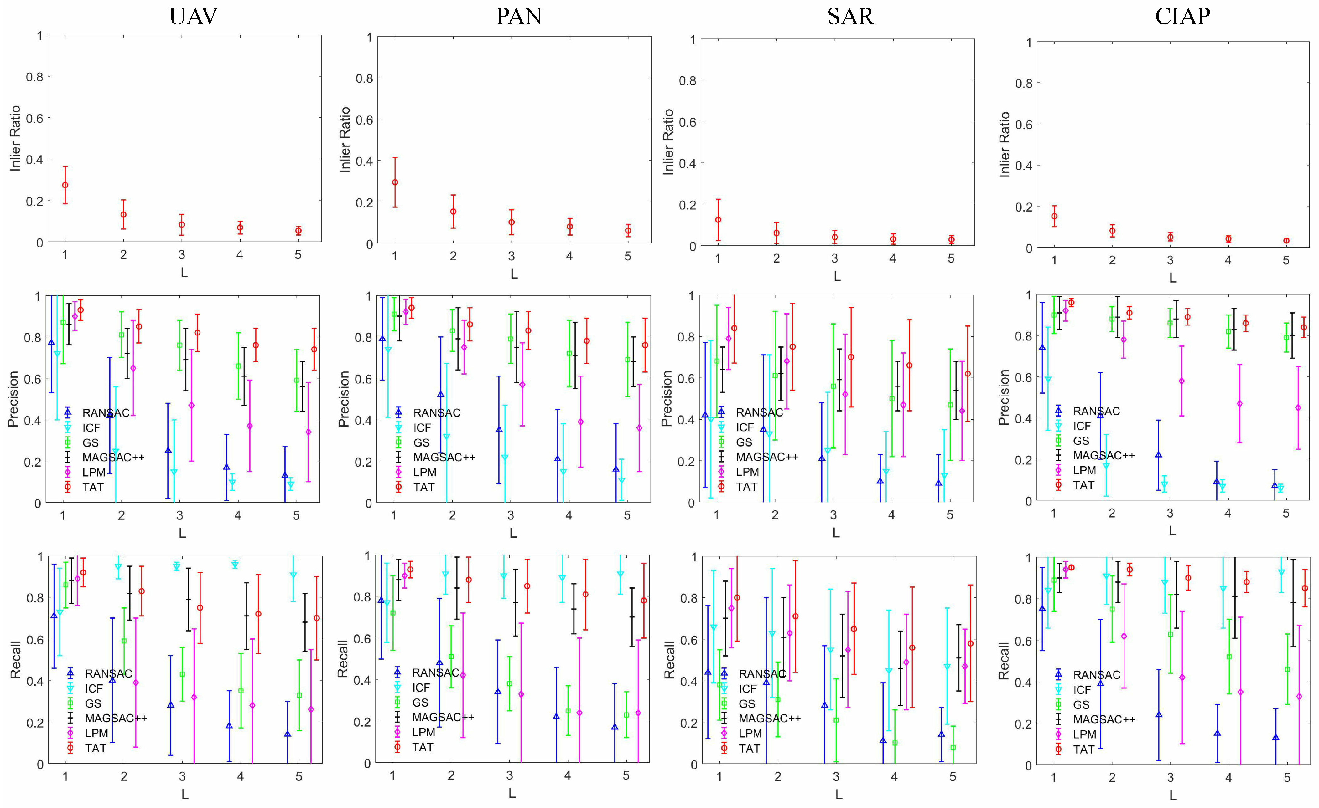
4.5. Robustness Test
We conducted robust experiments to test the robustness of our TAT. We keep the number of true matches in the hypothetical set constant, change the inlier ratio by increasing the number of hypothetical matches, and then test the matching performance of the above six methods separately. Specifically, for each feature point, we search the L most similar corresponding feature points with the SIFT. There are a total of N hypothetical matches in the hypothetical set in the case of the initial one-to-one feature point. Then, there are hypothetical matches in the hypothetical set when the corresponding number of feature points becomes one-to-L.
We set different
L values to obtain the mean of different inlier ratios in four remote-sensing datasets. As shown in
Table 1, clearly, the inlier ratio decreases with the increase of
L. In this way, we can increase the challenge of matching by increasing the number of false matches in the hypothetical set. On the other hand, searching for the
L most similar corresponding points may be more accurate to find the correct match. As the correct matching point corresponding to each feature point is not necessarily the first most similar point.
The robustness experiment results are shown in
Figure 9. The first row shows the mean and standard deviation of the different inlier ratios for the four remote-sensing datasets. From the precision and recall data shown in the second and third rows, respectively, we can clearly see that the matching performance of all methods deteriorates as the inlier rate decreases. Specifically, the precision and recall of RANSAC drop significantly on all four datasets. The precision of ICF is significantly reduced; however, the recall is relatively high. GS always maintains better results than RANSAC and ICF. MAGSAC++ also maintains better results because it is less affected by the interior point ratio. In contrast, TAT can maintain better and more stable matching performance than LPM and other methods.


