
Reliable Label-Supervised Pixel Attention Mechanism for Weakly Supervised Building Segmentation in UAV Imagery


1
School of Automation, China University of Geosciences, Wuhan 430074, China
2
Hubei Key Laboratory of Advanced Control and Intelligent Automation for Complex Systems, Wuhan 430074, China
3
Engineering Research Center of Intelligent Technology for Geo-Exploration, Ministry of Education, Wuhan 430074, China
4
Shanghai Institute of Technical Physics, Chinese Academy of Sciences, Shanghai 200083, China
5
Key Laboratory of Infrared System Detecting and Imaging Technology, Chinese Academy of Sciences, Shanghai 200083, China
6
Electronic Information School, Wuhan University, Wuhan 430072, China
7
Faculty of Engineering, China University of Geosciences, Wuhan 430074, China
*
Author to whom correspondence should be addressed.
Remote Sens. 2022, 14(13), 3196; https://0-doi-org.brum.beds.ac.uk/10.3390/rs14133196
Submission received: 13 May 2022
/
Revised: 27 June 2022
/
Accepted: 1 July 2022
/
Published: 3 July 2022
(This article belongs to the Special Issue Advances in Hyperspectral Remote Sensing: Methods and Applications)
Abstract
:Building segmentation for Unmanned Aerial Vehicle (UAV) imagery usually requires pixel-level labels, which are time-consuming and expensive to collect. Weakly supervised semantic segmentation methods for image-level labeling have recently achieved promising performance in natural scenes, but there have been few studies on UAV remote sensing imagery. In this paper, we propose a reliable label-supervised pixel attention mechanism for building segmentation in UAV imagery. Our method is based on the class activation map. However, classification networks tend to capture discriminative parts of the object and are insensitive to over-activation; therefore, class activation maps cannot directly guide segmentation network training. To overcome these challenges, we first design a Pixel Attention Module that captures rich contextual relationships, which can further mine more discriminative regions, in order to obtain a modified class activation map. Then, we use the initial seeds generated by the classification network to synthesize reliable labels. Finally, we design a reliable label loss, which is defined as the sum of the pixel-level differences between the reliable labels and the modified class activation map. Notably, the reliable label loss can handle over-activation. The preceding steps can significantly improve the quality of the pseudo-labels. Experiments on our home-made UAV data set indicate that our method can achieve 88.8% mIoU on the test set, outperforming previous state-of-the-art weakly supervised methods.
1. Introduction
Building segmentation plays an important role in digital cities, disaster assessment, and infrastructure planning and management. In recent years, with the development of UAV technology, building segmentation has become an important research direction in the high-resolution image segmentation field.
With the development of deep convolutional neural networks (DCNNs), the semantic segmentation task has witnessed great progress [1,2,3]. In the field of remote sensing, some segmentation methods based on DCNN have achieved excellent results in building segmentation, such as U-Net [4] and Deeplabv3+ [5]. All of these methods are based on precise pixel-level labels, which means that pixel-level labels are critical for training semantic segmentation networks. However, pixel-level labels are often lacking, and collecting them is a time-consuming and expensive task. Statistical results have shown that, for a 512 × 512 pixel remote sensing image, it takes 164.73 s to manually obtain pixel-level labels, while an image-level label only takes 1 s [6].
In order to address the lack of pixel-level labels, many studies have focused on the use of weakly supervised semantic segmentation (WSSS) for the semantic segmentation task [7,8]. WSSS can achieve pixel-level segmentation using only image-level labels.
WSSS methods are mainly based on the class activation map (CAM) [9]. The CAM trains the classification network through image-level labels, allowing the classifier to obtain the location maps of the target class. Although CAMs can recognize the most discriminative parts of objects, there are still three major obstacles that prevent them from being directly used as pseudo-labels for segmentation network training: (1) under-activation—CAMs tends to be highly responsive to parts of the object, rather than the whole region; (2) over-activation—the background region is incorrectly activated as the foreground; and (3) inconsistency—using different scaling transformations for the same input image can result in significant inconsistencies in the generated CAMs [10]. The root cause of these phenomena is the supervision gap between fully supervised and weakly supervised semantic segmentation.
In this paper, we propose a reliable label-supervised pixel attention mechanism (RSPA) to overcome the challenges associated with WSSS. We design rules for the generation of reliable labels. Reliable labels provide constraints that address the CAM over-activation problem. To solve the problem of under-activation in the original CAM, we introduce the pixel attention module (PAM) to obtain a modified CAM. We use the complementary relationship between the modified CAM and reliable labels to generate better pseudo-labels. We also design a reliable label loss, defined as the sum of the pixel-level differences between the reliable labels and the modified CAM. To address CAM inconsistency, we utilize the SEAM [10] equivariant regularization loss. The RSPA is implemented using a Siamese network structure with equivariant regularization loss.
The contributions of this work can be summarized as follows:
- 1.
- We propose a new, weakly supervised building segmentation network, RSPA, which can produce better pseudo-labels to train segmentation networks, resulting in better segmentation results.
- 2.
- We use the initial seeds to synthesize reliable labels, then use reliable labels as the constraints of the network to address CAM over-activation. PAM is proposed to capture long-range contextual information and find inter-pixel similarities. This can significantly enable the CAM to obtain more discriminative regions of the object.
- 3.
- The proposed reliable label loss takes full advantage of the complementary relationship between the modified CAM and reliable labels.
2. Related Works
In this section, we introduce fully supervised building segmentation methods and weakly supervised semantic segmentation for natural images and remote sensing images.
2.1. Fully Supervised Building Segmentation
In the past few years, with the development of deep learning techniques, many building segmentation methods based on convolutional neural networks have emerged [11].
Benefiting from their advantages in terms of the utilization of multi-level features, building segmentation methods based on encoder–decoder architectures have been widely used. For example, MA-FCN [12] and SiU-Net [13] are building segmentation networks based on FCN [14] and U-Net [4], respectively.
With the continuous development of segmentation models, dilated convolution, multi-scale pooling, and attention mechanisms have been introduced to enhance the robustness of segmentation networks to building scale changes. DSSNet [15] addresses the problem of resolution loss in hyperspectral images through the use of dilated convolutions, which has shown promising performance in hyperspectral image classification. Ji et al. [16] have embedded the Atrous Spatial Pyramid Pooling module [17] into a convolutional network, effectively improving the accuracy and robustness of building recognition. ASF-NET [18] uses an adaptive network structure to adjust the receptive field and enhance the useful feature information, thus obtaining high-precision building recognition results. All of the segmentation networks mentioned above require pixel-level labels as supervision in the training process; however, collecting pixel-level labels is time-consuming and expensive.
2.2. Weakly Supervised Semantic Segmentation
WSSS uses weak supervision, such as image-level labels [6,19], points [20,21], scribbles [22,23,24], and bounding boxes [25,26,27], in an attempt to achieve the same segmentation performance as fully supervised methods. Among these, image-level labels possess the weakest supervision information. In this paper, we study weakly supervised semantic segmentation based on image-level labels.
2.2.1. Weakly Supervised Semantic Segmentation of Natural Images
Adversarial erasing [19,28,29] involves erasing the most salient parts in the CAM, then driving the classification network to mine other salient regions from other regions. In [30,31], the affinity between pixels was calculated. In [32], a common attention classification network was proposed to discover complete object regions by processing cross-image semantics. SEAM [10] combines self-attention with equivariant regularization to ensure the consistency of the CAM under different transformations. BES [33] maintains the consistency of the segmentation and boundary by synthesizing boundary labels and providing boundary constraints; however, they are prone to over-activation because of their lack of constraints. In response, [34,35,36,37] have used saliency maps as constraints to address the problem of over-activation; however, saliency maps require additional costs, making them somewhat far from weakly supervised learning.
2.2.2. Weakly Supervised Semantic Segmentation of Remote Sensing Images
WSF-NET [6] uses a binary segmentation framework to solve the class imbalance problem and introduces a feature fusion network to adapt to the unique characteristics of targets in remote sensing images; however, this method does not consider the problem of over-activation and only hopes to find more target objects through a class balancing strategy and feature fusion network. SPMF-Net [38] takes image-level labels as supervision information in a classification network that combines superpixel pooling and multi-scale feature fusion structures. This method introduces superpixels as the supervision of the network in order to provide low-level feature information. This leads to the problem that the network depends on the accuracy of superpixel segmentation, and poor superpixels will lead to misclassification. U-CAM [21] uses image-level labels to generate CAMs. In contrast to other methods that only use image-level labels, this method introduces point-level labels as supervision to provide the location information of objects; however, these point-level labels require additional costs. CDSA [39] uses image-level labels to obtain location maps and provides structural information through the source domain. The structural information of the source domain can solve the problem of CAM over-activation. However, the acquisition of source domain structure information requires a large number of pixel-level labels, which is far from weakly supervised learning. Although the above methods have achieved remarkable results on remote sensing images, most of them lack consideration of the CAM over-activation issue. CDSA considers this issue but requires additional pixel-level labels as supervision.
In this paper, we not only solve CAM under-activation but also consider CAM over-activation by using only image-level labels.
3. Methodology
In this section, our method is described in detail. Figure 1 shows a popular weakly supervised segmentation process; our method also follows this route. Our WSSS method can be roughly divided into two stages: (1) synthesizing pseudo-labels of training images, given their image-level labels; and (2) training the segmentation model using the synthetic pseudo-labels. Here, our contributions are mainly in the first stage; namely, in terms of generating accurate pseudo-labels. Figure 2 shows our RSPA network framework.
3.1. Class Activation Map (CAM)
CAMs play an important role in WSSS, bridging between image and pixel-level labels. At present, most WSSS methods compute CAMs based on a convolutional neural network with Global Average Pooling before the last classification layer. In contrast to current WSSS methods, we propose to use Global Max Pooling (GMP) instead of Global Average Pooling (GAP) in the CAM network structure. As existing WSSS methods are commonly used in multi-class natural scene data sets, using GAP can motivate the network to find more discriminative regions of multiple categories. However, this paper mainly focuses on the binary segmentation of buildings, and using GMP is more in line with this demand. As GMP encourages the network to identify the most discriminative parts of the image, the low scores (noises) of the image regions are not taken into account when calculating the CAM. A class activation map from an image x can be computed as follows:
where denotes the weights of the final classification layer for class c, and is the feature map of x prior to GMP.
3.2. Synthesizing Reliable Labels
By changing the calculation method of CAM, the initial seeds can more accurately identify the discriminative regions of objects but still have the problems of over-activation and missing buildings. In order to eliminate over-activation and generate complete reliable labels, we design the following rules.
To obtain the complete reliable regions of the object, we first normalize the CAM calculated in Section 3.1 such that the maximum activation is equal to 1:
where B is the building class. Then, we design a background activation map, given by
where bg denotes the background and denotes a hyperparameter that adjusts background reliable scores. We reduce by increasing in Equation (3) such that the foreground scores dominate most regions of the CAM. Finally, dCRF [40] is applied to refine the CAM. dCRF encourages similar pixels to be assigned the same label, while pixels with large differences are assigned different labels.
The next step is to solve over-activation and obtain clear boundaries. The CAM calculated through the classification network is represented by pixel probabilities, where can be used to represent the probability that pixel i belongs to category B. As the CAM represented by pixel-wise class probability is not conducive to the synthesis of reliable labels, we use the threshold method to obtain the class label corresponding to each pixel. If is greater than the foreground threshold , the pixel i is a building label; otherwise, it is a background label.
We determine a sliding window of size , centered on pixel i. We use to represent the number of pixels allocated label B in the window. The proportion of this class in this window is defined as :
Pixel i will be marked as a reliable pixel if it meets the following criteria: if the proportion of class B in the window is greater than , then the pixel i will be identified as a reliable pixel. Formally, the reliable label for pixel i is computed as follows:
where is threshold for the condition. In particular, denotes that pixel i belongs to the reliable foreground, and denotes that pixel i belongs to the background.
3.3. Pixel Attention Module (PAM)
Although the CAM calculated in Section 3.1 can accurately cover the most discriminative regions in the target object, CAMs can only define parts of objects, rather than the whole region. To resolve CAM under-activation, we introduce the Pixel Attention Module.
As shown in Figure 2, we first obtain a high-level feature map by ResNet38 [41] as the input of the PAM, where the size of is of the input image. We do not consider low-level features, as low-level features in UAV images contain a lot of details. If a large amount of unfiltered detailed information is directly fused into the attention map, it will cause the network to learn the incorrect information, resulting in overfitting of the results.
We establish inter-pixel similarity through the following steps: (1) we feed the feature map into a convolution layer with a kernel size of 1 in order to obtain the feature maps Q and K. The feature values in position i of Q and K are denoted as and , respectively. We then multiply the matrices between the transpose of Q and K and apply the softmax layer to compute the attention map A:
where measures the similarity between the position and the position; denote the height, width, and channel sizes of feature maps, respectively; and is the number of pixels. Similar features of two pixels help to determine a greater correlation between them. (2) We feed the feature map into the convolution layer to obtain the feature map V. The feature value in position i of V is denoted as . The residual module is obtained by matrix multiplication of the feature map V and attention map A. We multiply the residual module by a hyperparameter and perform an element-wise sum operation with to obtain the final output ; see Figure 3), as follows:
where N is the number of pixels, j and i denote the positions of the feature map, and is initialized as 0 and gradually learns to assign more weights.
The PAM obtains global contextual information by extending the local features generated by the residual network, in order to establish rich contextual relations, and thus can mine more discriminative regions of the object.
3.4. Loss Design
- Classification loss: We use GMP at the end of the network to obtain the prediction probability vector p for image classification. To train the classification network, we use the binary cross-entropy loss function:where 0 and 1 denote background and foreground labels, respectively; denotes the classification label of sample i; and represents the number of training samples. As our network uses a Siamese network structure, the output includes two predictive probability vectors, and , where denotes the prediction probability vector of the original image and comes from the branch with the transformed image. The classification loss is the sum of the two branch results:
- Reliable label loss: The introduction of the PAM has the advantage of mining more discriminative regions, but it may also inevitably lead to over-activation. To take full advantage of the complementary relationship between the modified CAM and reliable labels, we use the Mean Square Error (MSE) as the loss function. In contrast to the Mean Absolute Error (MAE), MSE is sensitive to outliers, which correspond to over-activation. This advantage of MSE can allow us to address the over-activation of modified CAMs while preserving the complementary parts of the modified CAM and reliable labels. In the experimental results, we provide the quantitative results of reliable labels under different losses. In this paper, the loss function is defined as the pixel-level difference between the reliable labels and modified CAM, as follows:where M denotes the modified CAM and R denotes reliable label. Considering the two-branch structure of the Siamese Network, Equation (10) can be divided intowhere denotes the affine transformation, denotes the CAM obtained from the original input image, and denotes the CAM which comes from the branch with transformed image. The Reliable Label loss is the sum of the two branch results:
- Equivariant regularization loss (ER): In order to maintain the consistency of the output, equivariant regularization loss is considered:
The final loss of our network framework is defined as follows:
4. Experiments
4.1. Preparation for Experiments
4.1.1. Data Set
The Majiagou data set was collected using a DJI UAV platform in Majiagou, Zigui, Yichang, Hubei province, in March 2018. The resolution of the images is 6000 × 8000 pixels. The size of the data set is 600, covering an area of 3 square kilometers, including building types with different colors, sizes, and uses. Given the large scale of these images, the limited server performance, and the scattered distribution of buildings, we cropped the images into sub-images with a resolution of 1024 × 682 pixels. Finally, the processed Majiagou data set consisted of two classes, with 2031 and 704 images for training and testing, respectively.
4.1.2. Evaluation Metrics
In order to quantitatively analyze the comparison between our method and other methods, overall accuracy (OA), mean pixel intersection-over-union (mIoU), and over-activation rate (OAR) were adopted as the evaluation metrics. mIoU is defined as
IoU is defined as
and OA is defined as
where TP, FP, TN, FN, and c denote the numbers of true positives, false positives, true negatives, false negatives, and categories, respectively.
We found that the background often appears with the target object, leading to over-activation. To measure the degree of over-activation, we defined a metric
where is the number of pixels misclassified as the target class B (building class) for the background class , and is the number of true positive predictions of class B.
4.1.3. Implementation Details
We chose RetNet38 as our backbone network, with an output stride of 8. All backbone models were pre-trained on ImageNet [42]. During training, our RSPA was a shared-weight Siamese network. We used 5000 training iterations, with a learning rate of 0.0001 (0.01 for the last convolutional layer). Our method adopts rescaling with a downsampling rate of 0.6 during network training. We augmented the data through random scaling and flipping. For the segmentation network, we used the classical semantic segmentation model Deeplab-LargeFOV (V1) [43], where the backbone network was ResNet38. All experiments were performed on an NVIDIA GeForce GTX 3090 with 24G frame buffer.
4.2. Analysis of the RSPA
4.2.1. Improving the Quality of the Initial Seeds
The quality of the initial seeds helps to produce better pseudo-labels. However, the initial seeds generated by the original CAM have problems associated with over-activation and boundary blurring. To solve these problems, we used GMP instead of GAP before the last classification layer. In order to further analyze the improvement effect of GMP, we provide both quantitative and qualitative results relating to initial seeds under the different pooling methods (see Figure 4, Table 1). Compared with the initial seeds produced by GAP, the initial seeds produced by GMP increased the mIoU by 3.3%. From a qualitative point of view, the initial seeds produced by GAP cannot accurately identify narrow backgrounds between dense buildings, resulting in over-activation and a lack of clear boundaries (as shown in Figure 4, green boxes). The results indicate that the use of GMP can improve the quality of the initial seeds.
4.2.2. Comparison with Baseline (SEAM)
Table 2 details the ablation experiments considering each module. It shows that using the PAM module and a single branch network structure provided a significant improvement (of 3.4% over CAM and even 1.8% better than baseline). This proves that our method exceeds the baseline, even without using the Siamese Network and equivariant regularization. On this basis, the Siamese Network and equivariant regularization were added, and the mIoU of pseudo-labels was increased by 1.1%. Finally, with reliable label loss, the mIoU of our pseudo labels increased to 86.3%. This demonstrates the effectiveness of PAM and reliable label loss.
As shown in Figure 5, we compare our attention module (PAM) with the baseline attention module in our network framework. With the baseline attention module, pseudo-labels appeared to show overfitting in the network training (see Figure 5b,c). Background pixels are gradually misidentified as foreground. Better results were obtained with the PAM module.
4.2.3. Visualization of Pixel Attention Module
For the Pixel Attention Module, the attention map can be calculated by Equation (6), and its size is () × (), which means that, for each specific point in the image, there is a corresponding attention map corresponding to it, with size (H × W). As shown in Figure 6, the red crosses represent the selected pixel points. By observing their attention maps (the third column), it can be seen that the corresponding attention maps of these points highlight most of the areas where the buildings are located. To further demonstrate the effect of the Pixel Attention Module, we present the results of pseudo-labels with and without the Pixel Attention Module. As shown in Figure 7, with the Pixel Attention Module, the pseudo-label results were better. The Pixel Attention Module is more capable of capturing long-range dependencies and establishing inter-pixel similarity.
4.2.4. Handling over-Activation
Table 3 shows that, compared with other methods, the value of OAR calculated with our method was smaller, meaning that our method presented less over-activation. The pseudo-labels generated by our method can thus cover the target objects more accurately. Therefore, the pseudo-labels generated by our method are more consistent with the real segmentation labels.
4.2.5. Reliable Label Loss
4.3. Comparison with State-of-the-Art
4.3.1. Accuracy of Pseudo-Labels
In order to further elevate their accuracy, AffinityNet and IRN are usually used to refine pseudo-labels. Measuring the accuracy of the pseudo-labels is a common protocol in WSSS, as pseudo-labels of the train set are used to supervise the segmentation model. The quality of the pseudo-labels largely determines the final result of semantic segmentation. Table 5 summarizes the accuracy of the pseudo-labels, and it can be seen that our method was significantly better than the other methods. Our pseudo-labels increased the mIoU by 13.2% compared to the baseline. Our method achieved 86.25% without refinement. Figure 9 visualizes the pseudo-labels of our method and other methods. It can be seen that the problem of over-activation was more common in other methods, while our pseudo-labels had clearer boundaries and less over-activation.
4.3.2. Accuracy of Segmentation Maps
As shown in Table 5, the pseudo-labels we generated were accurate enough without any additional refinement. We used the pseudo-labels to train the classical segmentation model DeeplabV1 and obtained the final segmentation results. Table 6 and Figure 10 provide quantitative and qualitative results, respectively, demonstrating the superiority of our method. Compared to the baseline, our RSPA increased the mIoU by 6.7%. With our method, the mIoU reached 88.8% and the OA reached 98.5%. As shown in Figure 10, the comparison methods cannot accurately identify the narrow backgrounds between dense buildings, resulting in a loss of clear boundaries of buildings. Our results showed clear boundaries and could accurately segment buildings. Note that this performance improvement stemmed from our accurate pseudo-labels.
5. Discussion
As shown in Table 6, compared with the state-of-the-art WSSS methods, we obtained the best performance. Our mIoU (88.8%) was 6.7% higher than that of SEAM (82.1%). We argue that this performance improvement was due to the fact that we generated more accurate pseudo-labels. The quality of the pseudo-labels largely determines the final semantic segmentation result.
It can be seen from Figure 9 that over-activation and boundary blurring were common problems in the comparison methods. This is because most of the previous studies on WSSS methods have focused on solving CAM under-activation, while few studies have investigated the problem of CAM over-activation. There are also some methods that try to address CAM over-activation by adding constraints while solving the CAM under-activation; however, these methods do not appear to work well. As shown in Table 3, AffinityNet [30] had the most severe over-activation, as it mines discriminative regions by calculating the affinity between pixels but does not consider over-activation. IRN [31] and BES [33] have added boundary constraints on the basis of AffinityNet, but the effect of the boundary constraint is not ideal. The equivariant regularization proposed by SEAM [10] can inhibit over-activation, to a certain extent; however, the effect is not obvious. AdvCAM [44] solves the over-activation problem by introducing a regularization term to suppress the scores of the background categories. Compared to these methods, our method solves CAM over-activation more effectively. In order to solve the problem of over-activation, we first changed the CAM calculation method to obtain more accurate initial seeds. As shown in Figure 4, the initial seeds calculated by GAP presented obvious over-activation and blurred boundary problems, while the initial seeds calculated by GMP were better. Then, we used these initial seeds to synthesize reliable labels. Reliable labels provide constraints to overcome over-activation. To solve the problem of under-activation, we used PAM to capture long-range contextual information and find inter-pixel similarity (see Figure 7 and Figure 6). Table 2 details the improvements for each strategy in our method.
Although the pseudo-labels generated by our method achieved good results, there were still some problems. We can see from Figure 11 that the pseudo labels generated by our method could not identify all of the buildings in the image. Our pseudo-labels can accurately identify most of the buildings in the image, but when the color of the building is close to the color of the road and there is no obvious visual height difference, our method cannot separate the building from the background. Using such pseudo-labels to train a segmentation network will inevitably affect the segmentation result. In the future, we intend to address this issue and focus on how to generate more accurate pseudo-labels.
6. Conclusions
In this paper, we proposed a reliable label-supervised pixel attention mechanism for refining building segmentation in UAV imagery. We design a Pixel Attention Module (PAM), which refines the CAM through learning the inter-pixel similarity. Then, the initial seeds are used to synthesize reliable labels that provide the precise locations of buildings. Finally, we design a loss function by exploiting the complementary relationship between the modified CAM and reliable labels, in order to generate better pseudo-labels. Our RSPA was then implemented with a Siamese network structure. Compared with state-of-the-art WSSS methods, we obtained the best performance. Our future research will continue to focus on more efficient weakly supervised semantic segmentation methods.
Author Contributions
Conceptualization, J.C. and W.X.; methodology, J.C. and W.X.; software, W.X.; validation, W.X.; formal analysis, J.C., W.X., Y.Y., C.P. and W.G.; resources, J.C.; data curation, J.C.; writing—original draft preparation, W.X.; writing—review and editing, J.C., Y.Y., C.P. and W.G.; visualization, W.X.; supervision, J.C.; project administration, J.C.; funding acquisition, J.C. All authors have read and agreed to the published version of the manuscript.
Funding
This work was supported by the National Natural Science Foundation of China nos. 62073304, 41977242 and 61973283.
Data Availability Statement
Data are available from the authors upon reasonable request.
Conflicts of Interest
The authors declare no conflict of interest.
References
- Chen, L.C.; Papandreou, G.; Kokkinos, I.; Murphy, K.; Yuille, A.L. Deeplab: Semantic image segmentation with deep convolutional nets, atrous convolution, and fully connected crfs. IEEE Trans. Pattern Anal. Mach. Intell. 2017, 40, 834–848. [Google Scholar] [CrossRef] [PubMed] [Green Version]
- Peng, C.; Ma, J. Semantic segmentation using stride spatial pyramid pooling and dual attention decoder. Pattern Recognit. 2020, 107, 107498. [Google Scholar] [CrossRef]
- Peng, C.; Tian, T.; Chen, C.; Guo, X.; Ma, J. Bilateral attention decoder: A lightweight decoder for real-time semantic segmentation. Neural Netw. 2021, 137, 188–199. [Google Scholar] [CrossRef] [PubMed]
- Ronneberger, O.; Fischer, P.; Brox, T. U-net: Convolutional networks for biomedical image segmentation. In Proceedings of the International Conference on Medical Image Computing And Computer-Assisted Intervention, Munich, Germany, 5–9 October 2015; pp. 234–241. [Google Scholar]
- Chen, L.C.; Zhu, Y.; Papandreou, G.; Schroff, F.; Adam, H. Encoder-decoder with atrous separable convolution for semantic image segmentation. In Proceedings of the European Conference on Computer Vision, Munich, Germany, 8–14 September 2018; pp. 801–818. [Google Scholar]
- Fu, K.; Lu, W.; Diao, W.; Yan, M.; Sun, H.; Zhang, Y.; Sun, X. WSF-NET: Weakly supervised feature-fusion network for binary segmentation in remote sensing image. Remote Sens. 2020, 10, 1970. [Google Scholar] [CrossRef] [Green Version]
- Pathak, D.; Krahenbuhl, P.; Darrell, T. Constrained convolutional neural networks for weakly supervised segmentation. In Proceedings of the IEEE International Conference on Computer Vision, Santiago, Chile, 11–18 December 2015; pp. 1796–1804. [Google Scholar]
- Pinheiro, P.O.; Collobert, R. From image-level to pixel-level labeling with convolutional networks. In Proceedings of the IEEE Conference on Computer Vision and Pattern Recognition, Boston, MA, USA, 7–12 June 2015; pp. 1713–1721. [Google Scholar]
- Zhou, B.; Khosla, A.; Lapedriza, A.; Oliva, A.; Torralba, A. Learning deep features for discriminative localization. In Proceedings of the IEEE Conference on Computer Vision and Pattern Recognition, Las Vegas, NV, USA, 27–30 June 2016; pp. 2921–2929. [Google Scholar]
- Wang, Y.; Zhang, J.; Kan, M.; Shan, S.; Chen, X. Self-supervised equivariant attention mechanism for weakly supervised semantic segmentation. In Proceedings of the IEEE/CVF Conference on Computer Vision and Pattern Recognition, Seattle, WA, USA, 14–19 June 2020; pp. 12275–12284. [Google Scholar]
- Peng, C.; Zhang, K.; Ma, Y.; Ma, J. Cross Fusion Net: A Fast Semantic Segmentation Network for Small-Scale Semantic Information Capturing in Aerial Scenes. IEEE Trans. Geosci. Remote Sens. 2022, 60, 1–13. [Google Scholar] [CrossRef]
- Wei, S.; Ji, S.; Lu, M. Toward automatic building footprint delineation from aerial images using CNN and regularization. IEEE Trans. Geosci. Remote Sens. 2020, 58, 2178–2189. [Google Scholar] [CrossRef]
- Ji, S.; Wei, S.; Lu, M. Fully Convolutional Networks for Multisource Building Extraction from an Open Aerial and Satellite Imagery Data Set. IEEE Trans. Geosci. Remote Sens. 2019, 57, 574–586. [Google Scholar] [CrossRef]
- Long, J.; Shelhamer, E.; Darrell, T. Fully convolutional networks for semantic segmentation. In Proceedings of the IEEE Conference on Computer Vision and Pattern Recognition, Boston, MA, USA, 7–12 June 2015; pp. 3431–3440. [Google Scholar]
- Pan, B.; Xu, X.; Shi, Z.; Zhang, N.; Luo, H.; Lan, X. DSSNet: A Simple Dilated Semantic Segmentation Network for Hyperspectral Imagery Classification. IEEE Geosci. Remote. Sens. Lett. 2020, 17, 1968–1972. [Google Scholar] [CrossRef]
- Ji, S.; Wei, S.; Lu, M. A scale robust convolutional neural network for automatic building extraction from aerial and satellite imagery. Int. J. Remote Sens. 2019, 40, 3308–3322. [Google Scholar] [CrossRef]
- Chen, L.-C.; Papandreou, G.; Schroff, F.; Adam, H. Rethinking Atrous Convolution for Semantic Image Segmentation. arXiv 2017, arXiv:1706.05587. [Google Scholar]
- Chen, J.; Jiang, Y.; Luo, L.; Gong, W. ASF-Net: Adaptive Screening Feature Network for Building Footprint Extraction from Remote-Sensing Images. Int. J. Remote Sens. 2022, 60, 1–13. [Google Scholar] [CrossRef]
- Wei, Y.; Feng, J.; Liang, X.; Cheng, M.M.; Zhao, Y.; Yan, S. Object region mining with adversarial erasing: A simple classification to semantic segmentation approach. In Proceedings of the IEEE Conference on Computer Vision and Pattern Recognition, Honolulu, HI, USA, 21–26 July 2017; pp. 1568–1576. [Google Scholar]
- Bearman, A.; Russakovsky, O.; Ferrari, V.; Fei-Fei, L. What’s the point: Semantic segmentation with point supervision. In Proceedings of the European Conference on Computer Vision, Graz, Austria, 7–13 May 2016; pp. 549–565. [Google Scholar]
- Wang, S.; Chen, W.; Xie, S.M.; Azzari, G.; Lobell, D.B. Weakly supervised deep learning for segmentation of remote sensing imagery. Remote Sens. 2020, 12, 207. [Google Scholar] [CrossRef] [Green Version]
- Lin, D.; Dai, J.; Jia, J.; He, K.; Sun, J. Scribblesup: Scribble-supervised convolutional networks for semantic segmentation. In Proceedings of the IEEE Conference on Computer Vision and Pattern Recognition, Las Vegas, NV, USA, 27–30 June 2016; pp. 3159–3167. [Google Scholar]
- Vernaza, P.; Chandraker, M. Learning random-walk label propagation for weakly-supervised semantic segmentation. In Proceedings of the IEEE Conference on Computer Vision and Pattern Recognition, Honolulu, HI, USA, 21–26 July 2017; pp. 7158–7166. [Google Scholar]
- Wu, W.; Qi, H.; Rong, Z.; Liu, L.; Su, H. Scribble-supervised segmentation of aerial building footprints using adversarial learning. IEEE Access. 2018, 6, 58898–58911. [Google Scholar] [CrossRef]
- Song, C.; Huang, Y.; Ouyang, W.; Wang, L. Box-driven class-wise region masking and filling rate guided loss for weakly supervised semantic segmentation. In Proceedings of the IEEE/CVF Conference on Computer Vision and Pattern Recognition, Long Beach, CA, USA, 16–20 June 2019; pp. 3136–3145. [Google Scholar]
- Rafique, M.U.; Jacobs, N. Weakly Supervised Building Segmentation from Aerial Images. In Proceedings of the IGARSS 2019—2019 IEEE International Geoscience and Remote Sensing Symposium, Yokohama, Japan, 28 July–2 August 2019; pp. 3955–3958. [Google Scholar]
- Guo, R.; Sun, X.; Chen, K.; Zhou, X.; Yan, Z.; Diao, W.; Yan, M. Jmlnet: Joint multi-label learning network for weakly supervised semantic segmentation in aerial images. Remote Sens. 2020, 12, 3169. [Google Scholar] [CrossRef]
- Hou, Q.; Jiang, P.; Wei, Y.; Cheng, M.M. Self-erasing network for integral object attention. In Proceedings of the Advances in Neural Information Processing Systems, Vancouver, BC, Canada, 3–8 December 2018; pp. 549–559. [Google Scholar]
- Zhang, X.; Wei, Y.; Feng, J.; Yang, Y.; Huang, T.S. Adversarial complementary learning for weakly supervised object localization. In Proceedings of the IEEE Conference on Computer Vision and Pattern Recognition, Salt Lake City, UT, USA, 18–23 June 2018; pp. 1325–1334. [Google Scholar]
- Ahn, J.; Kwak, S. Learning pixel-level semantic affinity with image-level supervision for weakly supervised semantic segmentation. In Proceedings of the IEEE Conference on Computer Vision and Pattern Recognition, Salt Lake City, UT, USA, 18–23 June 2018; pp. 4981–4990. [Google Scholar]
- Ahn, J.; Cho, S.; Kwak, S. Weakly supervised learning of instance segmentation with inter-pixel relations. In Proceedings of the IEEE/CVF Conference on Computer Vision and Pattern Recognition, Long Beach, CA, USA, 16–20 June 2019; pp. 2209–2218. [Google Scholar]
- Sun, G.; Wang, W.; Dai, J.; Van Gool, L. Mining cross-image semantics for weakly supervised semantic segmentation. In Proceedings of the European Conference on Computer Vision, Glasgow, UK, 23–28 August 2020; Springer: Berlin/Heidelberg, Germany, 2020; pp. 347–365. [Google Scholar]
- Chen, L.; Wu, W.; Fu, C.; Han, X.; Zhang, Y. Weakly supervised semantic segmentation with boundary exploration. In Proceedings of the European Conference on Computer Vision, Glasgow, UK, 23–28 August 2020; pp. 347–362. [Google Scholar]
- Yao, Y.; Chen, T.; Xie, G.S.; Zhang, C.; Shen, F.; Wu, Q.; Tang, Z.; Zhang, J. Non-salient region object mining for weakly supervised semantic segmentation. In Proceedings of the IEEE Conference on Computer Vision and Pattern Recognition, Nashville, TN, USA, 19–25 June 2021; pp. 2623–2632. [Google Scholar]
- Yao, Q.; Gong, X. Saliency guided self-attention network for weakly and semi-supervised semantic segmentation. IEEE Access. 2020, 8, 14413–14423. [Google Scholar] [CrossRef]
- Lee, S.; Lee, M.; Lee, J.; Shim, H. Railroad is not a train: Saliency as pseudo-pixel supervision for weakly supervised semantic segmentation. In Proceedings of the IEEE Conference on Computer Vision and Pattern Recognition, Nashville, TN, USA, 19–25 June 2021; pp. 5495–5505. [Google Scholar]
- Zeng, Y.; Zhuge, Y.; Lu, H.; Zhang, L. Joint learning of saliency detection and weakly supervised semantic segmentation. In Proceedings of the IEEE/CVF International Conference on Computer Vision, Seoul, Korea, 27 October–2 November 2019; pp. 7223–7233. [Google Scholar]
- Chen, J.; He, F.; Zhang, Y.; Sun, G.; Deng, M. SPMF-Net: Weakly supervised building segmentation by combining superpixel pooling and multi-scale feature fusion. Remote Sens. 2020, 12, 1049. [Google Scholar] [CrossRef] [Green Version]
- Zhang, J.; Liu, Y.; Wu, P.; Shi, Z.; Pan, B. Mining Cross-Domain Structure Affinity for Refined Building Segmentation in Weakly Supervised Constraints. Remote Sens. 2022, 14, 1227. [Google Scholar] [CrossRef]
- Krahenbuhl, P.; Koltun, V. Efficient inference in fully connected crfs with gaussian edge potentials. In Proceedings of the 24th International Conference on Neural Information Processing Systems, Granada, Spain, 12–15 December 2011. [Google Scholar]
- Wu, Z.; Shen, C.; Van Den Hengel, A. Wider or deeper: Revisiting the resnet model for visual recognition. Pattern Recognit. 2019, 90, 119–133. [Google Scholar] [CrossRef] [Green Version]
- Deng, J.; Dong, W.; Socher, R.; Li, L.-J.; Li, K.; Li, F.-F. Imagenet: A large-scale hierarchical image database. In Proceedings of the IEEE Conference on Computer Vision and Pattern Recognition, Miami, FL, USA, 20–25 June 2009; pp. 248–255. [Google Scholar]
- Chen, L.C.; Kokkinos, I.; Murphy, K.; Yuille, A.L. Semantic image segmentation with deep convolutional nets and fully connected crfs. In Proceedings of the International Conference on Learning Representations, San Diego, CA, USA, 7–9 May 2015. [Google Scholar]
- Lee, J.; Kim, E.; Yoon, S. Anti-adversarially manipulated attributions for weakly and semi-supervised semantic segmentation. In Proceedings of the IEEE Conference on Computer Vision and Pattern Recognition, Nashville, TN, USA, 19–25 June 2021; pp. 4071–4080. [Google Scholar]
Figure 1.
Weakly supervised segmentation: (a) Stage 1. Synthesizing pseudo-labels by weak supervision; and (b) Stage 2. Using pseudo-labels to supervise segmentation network training.
Figure 1.
Weakly supervised segmentation: (a) Stage 1. Synthesizing pseudo-labels by weak supervision; and (b) Stage 2. Using pseudo-labels to supervise segmentation network training.

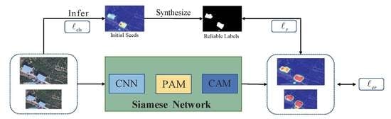
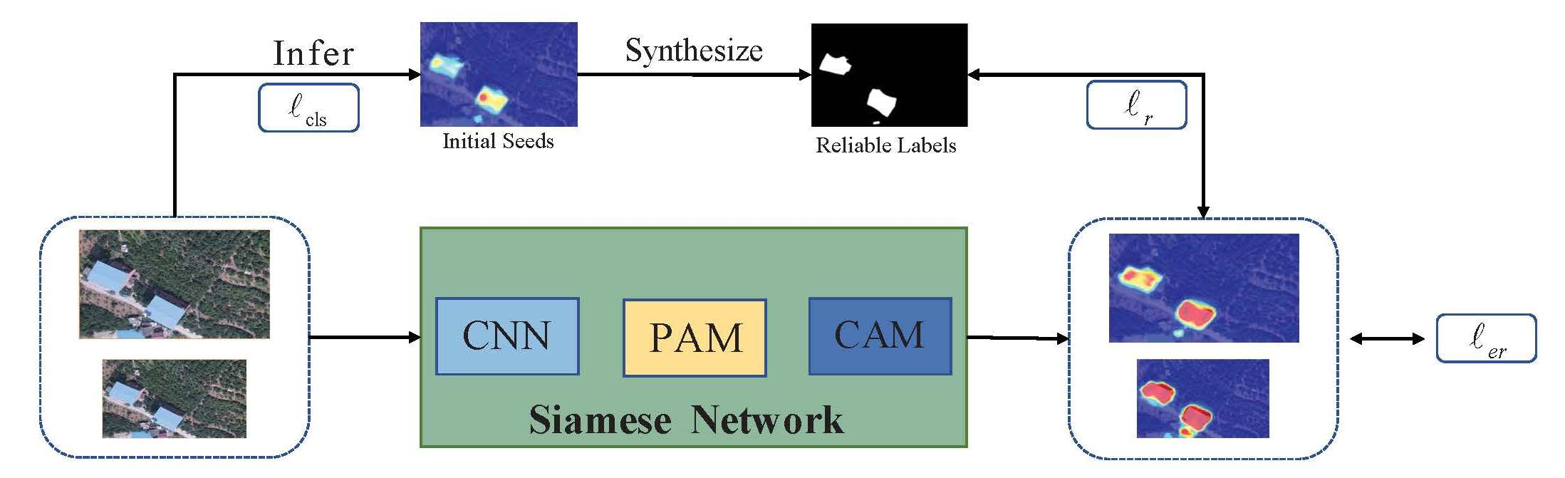
Figure 2.
Our proposed RSPA framework is based on a Siamese network. First, the initial seeds are obtained through the classification network, which are then used to synthesize reliable labels. PAM can further mine more discriminative regions to obtain modified CAMs. The RSPA is the integration of PAM and reliable label supervision. GMP denotes Global Max Pooling. The affine transformation is rescaling.

Figure 3.
Pixel Attention Module. denote height, width, and channel sizes of feature maps, respectively, and k denotes the kernel size.
Figure 3.
Pixel Attention Module. denote height, width, and channel sizes of feature maps, respectively, and k denotes the kernel size.

Figure 4.
Different pooling methods of initial seeds on Majiagou data set training images. The green boxes represent regions of boundary blurring: (a) images; (b) ground truth; (c) initial seeds with GAP; and (d) initial seeds with GMP.
Figure 4.
Different pooling methods of initial seeds on Majiagou data set training images. The green boxes represent regions of boundary blurring: (a) images; (b) ground truth; (c) initial seeds with GAP; and (d) initial seeds with GMP.

Figure 5.
Pseudo-labels obtained with different modules: (a) image; (b) pseudo-labels with baseline attention module (1000 iterations); (c) pseudo-labels with baseline attention module (5000 iterations); (d) ground truth; (e) pseudo-labels with PAM (1000 iterations); and (f) pseudo-labels with PAM (5000 iterations). The green box represents regions of over-activation.

Figure 6.
The visualization of attention maps: (a) images; (b) ground truth; and (c) attention maps. Note that the red crosses denote the selected pixels, and blue pixels in the attention map represent similar features.
Figure 6.
The visualization of attention maps: (a) images; (b) ground truth; and (c) attention maps. Note that the red crosses denote the selected pixels, and blue pixels in the attention map represent similar features.

Figure 7.
Visualization results of Pixel Attention Module: (a) images; (b) ground truth; (c) pseudo-labels without PAM; and (d) pseudo-labels with PAM.
Figure 7.
Visualization results of Pixel Attention Module: (a) images; (b) ground truth; (c) pseudo-labels without PAM; and (d) pseudo-labels with PAM.

Figure 8.
Results of pseudo-labels at different losses: (a) image; (b) ground truth; (c) reliable label; (d) modified CAM; (e) pseudo-label with MAE; and (f) pseudo-label with MSE. Note that the pseudo-label with MSE was better than the pseudo-label with MAE.
Figure 8.
Results of pseudo-labels at different losses: (a) image; (b) ground truth; (c) reliable label; (d) modified CAM; (e) pseudo-label with MAE; and (f) pseudo-label with MSE. Note that the pseudo-label with MSE was better than the pseudo-label with MAE.

Figure 9.
Qualitative comparison of pseudo-labels on Majiagou training set: (a) images; (b) ground truth; (c) AffinityNet; (d) IRN; (e) SEAM; (f) BES; (g) AdvCAM; and (h) ours.
Figure 9.
Qualitative comparison of pseudo-labels on Majiagou training set: (a) images; (b) ground truth; (c) AffinityNet; (d) IRN; (e) SEAM; (f) BES; (g) AdvCAM; and (h) ours.

Figure 10.
Qualitative comparison of segmentation results on Majiagou test set. (a) Images; (b) ground-truth; (c) AffinityNet; (d) IRN; (e) SEAM; (f) BES; (g) AdvCAM; and (h) ours.
Figure 10.
Qualitative comparison of segmentation results on Majiagou test set. (a) Images; (b) ground-truth; (c) AffinityNet; (d) IRN; (e) SEAM; (f) BES; (g) AdvCAM; and (h) ours.

Figure 11.
Comparison of pseudo-labels. Red boxes represent regions of under-activation: (a) image; (b) ground truth; and (c) pseudo-labels.
Figure 11.
Comparison of pseudo-labels. Red boxes represent regions of under-activation: (a) image; (b) ground truth; and (c) pseudo-labels.


Table 1.
mIoU (%) of the initial seeds on Majiagou data set training images.
| Method | Initial Seeds |
|---|---|
| CAM (GAP) | 74.9 |
| CAM (GMP) | 78.2 |
Table 2.
Ablation experiments for each part of RSPA. PAM, Pixel Attention Module; SN, Siamese Network; ER, equivariant regularization.
Table 2.
Ablation experiments for each part of RSPA. PAM, Pixel Attention Module; SN, Siamese Network; ER, equivariant regularization.
| Baseline | CAM | PAM | SN and ER | Reliable Label Loss | mIoU (%) |
|---|---|---|---|---|---|
| ✓ | 79.8 | ||||
| ✓ | 78.2 | ||||
| ✓ | ✓ | 81.6 | |||
| ✓ | ✓ | ✓ | 82.7 | ||
| ✓ | ✓ | ✓ | ✓ | 86.3 |
Table 3.
Comparison with state-of-the-art methods for handling the over-activation problem. OAR (%; the lower the better). IoU (%; the higher the better).
Table 3.
Comparison with state-of-the-art methods for handling the over-activation problem. OAR (%; the lower the better). IoU (%; the higher the better).
| Method | OAR | IoU |
|---|---|---|
| AffinityNet [30] | 65.50 | 57.42 |
| IRN [31] | 50.19 | 64.84 |
| SEAM (Baseline) [10] | 48.75 | 65.24 |
| BES [33] | 53.86 | 63.22 |
| AdvCAM [44] | 35.47 | 70.10 |
| Ours | 22.36 | 75.53 |
Table 4.
mIoU (%) of the pseudo-labels with different loss functions.
| Loss Function | mIoU |
|---|---|
| MAE | 84.24 |
| MSE | 86.25 |
Table 5.
Accuracy (mIoU%) of pseudo-labels evaluated on the Majiagou training set. The best score is shown in bold throughout all experiments.
Table 5.
Accuracy (mIoU%) of pseudo-labels evaluated on the Majiagou training set. The best score is shown in bold throughout all experiments.
| Method | w/o Refinement | w/AffinityNet | w/IRN |
|---|---|---|---|
| AffinityNet [30] | 74.89 | - | - |
| IRN [31] | 79.53 | - | - |
| SEAM (Baseline) [10] | 73.05 | 79.80 | - |
| BES [33] | 78.52 | - | - |
| AdvCAM [44] | 76.17 | - | 82.25 |
| Ours | 86.25 | - | - |
Table 6.
Segmentation results on the Majiagou test set. The best score is in bold throughout all experiments.
Publisher’s Note: MDPI stays neutral with regard to jurisdictional claims in published maps and institutional affiliations. |
© 2022 by the authors. Licensee MDPI, Basel, Switzerland. This article is an open access article distributed under the terms and conditions of the Creative Commons Attribution (CC BY) license (https://creativecommons.org/licenses/by/4.0/).
Share and Cite
MDPI and ACS Style
Chen, J.; Xu, W.; Yu, Y.; Peng, C.; Gong, W. Reliable Label-Supervised Pixel Attention Mechanism for Weakly Supervised Building Segmentation in UAV Imagery. Remote Sens. 2022, 14, 3196. https://0-doi-org.brum.beds.ac.uk/10.3390/rs14133196
AMA Style
Chen J, Xu W, Yu Y, Peng C, Gong W. Reliable Label-Supervised Pixel Attention Mechanism for Weakly Supervised Building Segmentation in UAV Imagery. Remote Sensing. 2022; 14(13):3196. https://0-doi-org.brum.beds.ac.uk/10.3390/rs14133196
Chicago/Turabian StyleChen, Jun, Weifeng Xu, Yang Yu, Chengli Peng, and Wenping Gong. 2022. "Reliable Label-Supervised Pixel Attention Mechanism for Weakly Supervised Building Segmentation in UAV Imagery" Remote Sensing 14, no. 13: 3196. https://0-doi-org.brum.beds.ac.uk/10.3390/rs14133196
Note that from the first issue of 2016, this journal uses article numbers instead of page numbers. See further details here.