
Worldwide Statistical Correlation of Eight Years of Swarm Satellite Data with M5.5+ Earthquakes: New Hints about the Preseismic Phenomena from Space

 ,
,  ,
,  , , , , , ,
  ,
,
Abstract
:
1. Introduction
2. Materials and Methods
2.1. Investigated Datasets
2.1.1. Satellite Datasets
2.1.2. Earthquake Catalog Acquisition and Pre-Processing
2.2. Methods of Analysis
- First differences of the data: the difference between two consecutive data divided by the time interval between them (as a first order approximation of the temporal derivative).
- Removal of the residual trend: a cubic spline coming from the fitting of the derivative of the data (as obtained from Step 1) is removed.
- Analysis of the residuals obtained from Step 1 and Step 2 along the track: moving windows of 7° latitude are used, with an incremental shift of 1/5 of the window length (i.e., ~1.4° of latitude).
- The root mean square (rms) is calculated inside the window and compared with the whole track’s Root Mean Square (RMS). The anomaly is defined if ( is chosen as 2.5 or 3 if no-frequency investigation is performed; more details are given later on).
- Method 1 “All anomalies–EQs”. This method selects all earthquakes compatible with the investigated anomaly. The advantage is that we do not apply any assumption for the analysis, and we can suppose that, in case the statistics are sufficient, the “wrong” anomaly–earthquake couples increase just the background without creating additional artificial concentrations of anomalies. On the other side, one disturbance can be produced only by one earthquake, and so, unless the signal is superposed (or under the satellite resolution), the anomaly could not be associated with more than one event. For this reason, we also introduce the following methods.
- Method 2 “Min [log(ΔT R)]”. This method selects the closest earthquake in space (“R”) and time (anticipation time ΔT ). The selection is made by searching for the minimum of the following equation: log10(|ΔT∙R|). The criterion is based on the assumption that an anomaly is more likely to be produced by the closest earthquake in space and time.
- Method 3 “Max (magnitude)”. This method selects the earthquake with the highest magnitude in the space and time domains of interest. The assumption is that a larger earthquake produces more anomalies before its occurrence that can be detectable in the ionosphere.
- Method 4 “Closer (Rikitake)”. This method takes into account that a larger earthquake with a magnitude M is expected to have a longer anticipation time of its possible precursors, according to the Rikitake law [37], expressed as:
3. Results
3.1. Swarm Magnetic Field Results
3.2. Swarm Electron Density Results
4. Discussion
4.1. General Comparison for Magnetic Field and Ne Results
4.2. Validation of the Results by Confusion Matrix Performance Evaluation and ROC Curves
- True positive (TP): in the cell, there is at least an anomaly, and an earthquake follows within the next 90 days
- True negative (TN): in the cell, there are no anomalies, and no earthquakes follow in the next 90 days in the same cell.
- False positive (FP): in the cell, there is one or more anomalies, and no earthquakes follow in the next 90 days in the same cell
- False negative (FN): in the cell, there are no anomalies, and an earthquake follows in the next 90 days.
4.3. Improving the Superposed Epoch Approach by Taking into Account the Rikitake Law
4.4. Some Features of the Largest Concentrations
4.5. General Comparison of the Number of “Pre-“ and “Post-“ Earthquake Anomalies
5. Conclusions
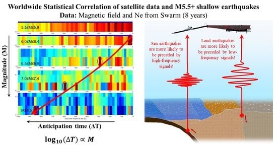
- The anticipation time “” of the anomaly increases with the magnitude of the incoming earthquakes following the Rikitake laws [37], with these specific coefficients being and for the magnetic field “mag” and electron density data, respectively. The anticipation time of large earthquakes (M7.5+) seems to be some years before the event and has been detected.
- The focal mechanism seems to have a small or null influence on the generated frequency of the possible pre-earthquake anomalies.
- Earthquakes localized in the land areas tend to be preceded by lower frequency anomalous signals, while sea earthquakes are more likely to be preceded by faster signal anomalies.
- The Swarm magnetic field signal anomalies generally show a better correlation with earthquakes than the electron density ones do.
- A more selective set of parameters, achieved here by the investigation of the signal frequency, reduces the size of the anomaly dataset, and it is shown that the possible correlation with the seismic event has a higher statistical significance for both the magnetic field and Ne observations.
- Frequency analysis seems to be fundamental in some cases: for electron density, we find a higher correlation with anomalies, with a signal period in the range of 25–50 s.
- All the results in this paper have been tested with the “confusion matrix” approach, reaching an accuracy from 75% to 95% and an alarmed time-space from 0.7% to 19.1%. The real results show a predicting capability that is 1.67 times better than that of a random predictor, according to the AUC of the ROC curve, which further proves a prediction capability of the best detected ionospheric anomalies by WSC.
Supplementary Materials
Author Contributions
Funding
Data Availability Statement
Acknowledgments
Conflicts of Interest
Appendix A. Evaluation of the Declustering of the Earthquake Catalog on the Worldwide Statistical Correlation Results

References
- Rikitake, T. Classification of earthquake precursors. Tectonophysics 1979, 54, 293–309. [Google Scholar] [CrossRef]
- Conti, L.; Picozza, P.; Sotgiu, A. A Critical Review of Ground Based Observations of Earthquake Precursors. Front. Earth Sci. 2021, 9, 676766. [Google Scholar] [CrossRef]
- Picozza, P.; Conti, L.; Sotgiu, A. Looking for Earthquake Precursors From Space: A Critical Review. Front. Earth Sci. 2021, 9. [Google Scholar] [CrossRef]
- Fraser-Smith, A.C.; Bernardi, A.; McGill, P.R.; Ladd, M.E.; Helliwell, R.A.; Villard, O.G., Jr. Low-frequency magnetic field measurements near the epicenter of the Ms7.1 Loma Prieta Earthquake. Geophys. Res. Lett. 1990, 17, 1465–1468. [Google Scholar] [CrossRef]
- Molchanov, O.A.; Kopytenko, Y.A.; Voronov, P.M.; Matiashvili, T.G.; Fraser-Smith, A.C.; Bernardi, A. Results of ULF magnetic field measurements near the epicenters of the Spitak (Ms = 6.9) and Loma Prieta (Ms = 7.1) earthquakes: Comparative analysis. Geophys. Res. Lett. 1992, 19, 1495–1498. [Google Scholar] [CrossRef]
- Molchanov, O.A.; Hayakawa, M. Generation of ULF electromagnetic emissions by microfracturing. Geophys. Res. Lett. 1995, 22, 3091–3094. [Google Scholar] [CrossRef]
- Molchanov, O.; Hayakawa, M. On the generation mechanism of ULF seismogenic electromagnetic emissions. Phys. Earth Planet. Inter. 1998, 105, 201–210. [Google Scholar] [CrossRef]
- Freund, F.T. Pre-earthquake signals: Underlying physical processes. J. Southeast Asian Earth Sci. 2011, 41, 383–400. [Google Scholar] [CrossRef]
- Freund, F.; Ouillon, G.; Scoville, J.; Sornette, D. Earthquake precursors in the light of peroxy defects theory: Critical review of systematic observations. Eur. Phys. J. Spec. Top. 2021, 230, 7–46. [Google Scholar] [CrossRef]
- Kuo, C.L.; Lee, L.C.; Huba, J.D. An improved coupling model for the lithosphere-atmosphere-ionosphere system. J. Geophys. Res. Space Phys. 2014, 119, 3189–3205. [Google Scholar] [CrossRef]
- Kuo, C.-L.; Ho, Y.-Y.; Lee, L.-C. Electrical Coupling Between the Ionosphere and Surface Charges in the Earthquake Fault Zone. In Pre-Earthquake Processes: A Multidisciplinary Approach to Earthquake Prediction Studies; John Wiley & Sons, Inc.: Hoboken, NJ, USA, 2018; pp. 99–124. [Google Scholar] [CrossRef]
- Prokhorov, B.E.; Zolotov, O.V. Comment on “An improved coupling model for the lithosphere-atmosphere-ionosphere system” by Kuo et al. [2014]. J. Geophys. Res. Space Phys. 2017, 122, 4865–4868. [Google Scholar] [CrossRef] [Green Version]
- Kuo, C.-L.; Lee, L.-C. Reply to comment by B. E. Prokhorov and O. V. Zolotov on “An improved coupling model for the lithosphere-atmosphere-ionosphere system”. J. Geophys. Res. Space Phys. 2017, 122, 4869–4874. [Google Scholar] [CrossRef] [Green Version]
- Denisenko, V.V.; Boudjada, M.Y.; Lammer, H. Propagation of Seismogenic Electric Currents Through the Earth’s Atmosphere. J. Geophys. Res. Space Phys. 2018, 123, 4290–4297. [Google Scholar] [CrossRef] [Green Version]
- Denisenko, V.V.; Nesterov, S.A.; Boudjada, M.Y.; Lammer, H. A mathematical model of quasistationary electric field penetration from ground to the ionosphere with inclined magnetic field. J. Atmospheric Sol.-Terr. Phys. 2018, 179, 527–537. [Google Scholar] [CrossRef]
- Pulinets, S.A.; Ouzounov, D. Lithosphere–Atmosphere–Ionosphere Coupling (LAIC) model—An unified concept for earthquake precursors validation. J. Asian Earth Sci. 2011, 41, 371–382. [Google Scholar] [CrossRef]
- Scholz, C.H.; Sykes, L.R.; Aggarwal, Y.P. Earthquake Prediction: A Physical Basis. Science 1973, 181, 803–810. [Google Scholar] [CrossRef]
- Ventura, G.; Di Giovambattista, R. Fluid pressure, stress field and propagation style of coalescing thrusts from the analysis of the 20 May 2012 ML5.9 Emilia earthquake (Northern Apennines, Italy). Terra Nova 2013, 25, 72–78. [Google Scholar] [CrossRef]
- Fidani, C.; Orsini, M.; Iezzi, G.; Vicentini, N.; Stoppa, F. Electric and Magnetic Recordings by Chieti CIEN Station During the Intense 2016–2017 Seismic Swarms in Central Italy. Front. Earth Sci. 2020, 8, 536332. [Google Scholar] [CrossRef]
- Marchetti, D.; De Santis, A.; D’Arcangelo, S.; Poggio, F.; Jin, S.; Piscini, A.; Campuzano, S.A. Magnetic Field and Electron Density Anomalies from Swarm Satellites Preceding the Major Earthquakes of the 2016–2017 Amatrice-Norcia (Central Italy) Seismic Sequence. Pure Appl. Geophys. 2019, 177, 305–319. [Google Scholar] [CrossRef]
- Liperovsky, V.A.; Pokhotelov, O.A.; Meister, C.-V.; Liperovskaya, E.V. Physical models of coupling in the lithosphere-atmosphere-ionosphere system before earthquakes. Geomagn. Aeron. 2008, 48, 795–806. [Google Scholar] [CrossRef]
- Parrot, M.; Li, M. Demeter results related to seismic activity. URSI Radio Sci. Bull. 2015, 2015, 18–25. [Google Scholar] [CrossRef]
- Yan, R.; Parrot, M.; Pinçon, J.-L. Statistical Study on Variations of the Ionospheric Ion Density Observed by DEMETER and Related to Seismic Activities. J. Geophys. Res. Space Phys. 2017, 122, 12421–12429. [Google Scholar] [CrossRef] [Green Version]
- Ouyang, X.Y.; Parrot, M.; Bortnik, J. ULF Wave Activity Observed in the Nighttime Ionosphere Above and Some Hours Before Strong Earthquakes. J. Geophys. Res. Space Phys. 2020, 125, e2020JA028396. [Google Scholar] [CrossRef]
- Zolotov, O.V. Ionosphere quasistatic electric fields disturbances over seismically active regions as inferred from satellite-based observations: A review. Russ. J. Phys. Chem. B 2015, 9, 785–788. [Google Scholar] [CrossRef]
- Akhoondzadeh, M.; De Santis, A.; Marchetti, D.; Piscini, A.; Jin, S. Anomalous seismo-LAI variations potentially associated with the 2017 Mw = 7.3 Sarpol-e Zahab (Iran) earthquake from Swarm satellites, GPS-TEC and climatological data. Adv. Space Res. 2019, 64, 143–158. [Google Scholar] [CrossRef]
- De Santis, A.; Marchetti, D.; Spogli, L.; Cianchini, G.; Pavón-Carrasco, F.J.; De Franceschi, G.; Di Giovambattista, R.; Perrone, L.; Qamili, E.; Cesaroni, C.; et al. Magnetic Field and Electron Density Data Analysis from Swarm Satellites Searching for Ionospheric Effects by Great Earthquakes: 12 Case Studies from 2014 to 2016. Atmosphere 2019, 10, 371. [Google Scholar] [CrossRef] [Green Version]
- Marchetti, D.; De Santis, A.; Campuzano, S.A.; Soldani, M.; Piscini, A.; Sabbagh, D.; Cianchini, G.; Perrone, L.; Orlando, M. Swarm Satellite Magnetic Field Data Analysis Prior to 2019 Mw = 7.1 Ridgecrest (California, USA) Earthquake. Geosciences 2020, 10, 502. [Google Scholar] [CrossRef]
- De Santis, A.; Marchetti, D.; Pavón-Carrasco, F.J.; Cianchini, G.; Perrone, L.; Abbattista, C.; Alfonsi, L.; Amoruso, L.; Campuzano, S.A.; Carbone, M.; et al. Precursory worldwide signatures of earthquake occurrences on Swarm satellite data. Sci. Rep. 2019, 9, 20287. [Google Scholar] [CrossRef] [Green Version]
- De Santis, A.; Marchetti, D.; Perrone, L.; Campuzano, S.A.; Cianchini, G.; Cesaroni, C.; Di Mauro, D.; Orlando, M.; Piscini, A.; Sabbagh, D.; et al. Statistical correlation analysis of strong earthquakes and ionospheric electron density anomalies as observed by CSES-01. Nuovo Cim. C 2021, 44, 1–4. [Google Scholar] [CrossRef]
- Friis-Christensen, E.; Lühr, H.; Hulot, G. Swarm: A constellation to study the Earth’s magnetic field. Earth Planets Space 2006, 58, 351–358. [Google Scholar] [CrossRef] [Green Version]
- Pinheiro, K.J.; Jackson, A.; Finlay, C.C. Measurements and uncertainties of the occurrence time of the 1969, 1978, 1991, and 1999 geomagnetic jerks. Geochem. Geophys. Geosyst. 2011, 12, Q10015. [Google Scholar] [CrossRef]
- Yan, R.; Zhima, Z.; Xiong, C.; Shen, X.; Huang, J.; Guan, Y.; Zhu, X.; Liu, C. Comparison of Electron Density and Temperature From the CSES Satellite With Other Space-Borne and Ground-Based Observations. J. Geophys. Res. Space Phys. 2020, 125, e2019ja027747. [Google Scholar] [CrossRef]
- Marchetti, D.; De Santis, A.; Shen, X.; Campuzano, S.A.; Perrone, L.; Piscini, A.; Di Giovambattista, R.; Jin, S.; Ippolito, A.; Cianchini, G.; et al. Possible Lithosphere-Atmosphere-Ionosphere Coupling effects prior to the 2018 Mw = 7.5 Indonesia earthquake from seismic, atmospheric and ionospheric data. J. Southeast Asian Earth Sci. 2019, 188, 104097. [Google Scholar] [CrossRef]
- Reasenberg, P. Second-order moment of central California seismicity, 1969–1982. J. Geophys. Res. Earth Surf. 1985, 90, 5479–5495. [Google Scholar] [CrossRef]
- Dobrovolsky, I.P.; Zubkov, S.I.; Miachkin, V.I. Estimation of the size of earthquake preparation zones. Pure Appl. Geophys. 1979, 117, 1025–1044. [Google Scholar] [CrossRef]
- Rikitake, T. Earthquake precursors in Japan: Precursor time and detectability. Tectonophysics 1987, 136, 265–282. [Google Scholar] [CrossRef]
- Song, R.; Hattori, K.; Zhang, X.; Liu, J.; Yoshino, C. Detecting the Ionospheric Disturbances in Japan Using the Three-Dimensional Computerized Tomography. J. Geophys. Res. Space Phys. 2021, 126, e2020ja028561. [Google Scholar] [CrossRef]
- Shcherbakov, R.; Turcotte, D.L.; Rundle, J.B.; Tiampo, K.F.; Holliday, J.R. Forecasting the Locations of Future Large Earthquakes: An Analysis and Verification. Pure Appl. Geophys. 2010, 167, 743–749. [Google Scholar] [CrossRef] [Green Version]
- Xiong, P.; Marchetti, D.; De Santis, A.; Zhang, X.; Shen, X. SafeNet: SwArm for Earthquake Perturbations Identification Using Deep Learning Networks. Remote Sens. 2021, 13, 5033. [Google Scholar] [CrossRef]
- Fawcett, T. An Introduction to ROC analysis. Pattern Recogn. Lett. 2006, 27, 861–874. [Google Scholar] [CrossRef]
- Gutenberg, B.; Richter, C.F. Seismicity of the Earth and Associated Phenomena, 2nd ed.; Princeton University Press: Princeton, NJ, USA, 1954. [Google Scholar]
- McLaskey, G.C. Earthquake Initiation From Laboratory Observations and Implications for Foreshocks. J. Geophys. Res. Solid Earth 2019, 124, 12882–12904. [Google Scholar] [CrossRef]
- Scholz, C. The Mechanics of Earthquakes and Faulting, 3rd ed.; Cambridge University Press: Cambridge, UK, 2019. [Google Scholar] [CrossRef] [Green Version]
- Kachakhidze, M.K.; Kachakhidze, N.K.; Kaladze, T.D. A model of the generation of electromagnetic emissions detected prior to earthquakes. Phys. Chem. Earth Parts A/B/C 2015, 85–86, 78–81. [Google Scholar] [CrossRef] [Green Version]
- He, Y.; Zhao, X.; Yang, D.; Wu, Y.; Li, Q. A study to investigate the relationship between ionospheric disturbance and seismic activity based on Swarm satellite data. Phys. Earth Planet. Inter. 2021, 323, 106826. [Google Scholar] [CrossRef]
- Dziewonski, A.M.; Chou, T.-A.; Woodhouse, J.H. Determination of earthquake source parameters from waveform data for studies of global and regional seismicity. J. Geophys. Res. Earth Surf. 1981, 86, 2825–2852. [Google Scholar] [CrossRef]
- Ekström, G.; Nettles, M.; Dziewoński, A. The global CMT project 2004–2010: Centroid-moment tensors for 13,017 earthquakes. Phys. Earth Planet. Inter. 2012, 200, 1–9. [Google Scholar] [CrossRef]
- Cronin Vincent, S. A Primer on Focal Mechanism Solutions for Geologists. Lecture 11 of “OCEAN/ESS 410, Fall 2014 Marine Geology and Geophysics”. 2010. Available online: https://www.ocean.washington.edu/courses/oc410/backgroundreading.html (accessed on 8 January 2022).
- Zhu, K.; Fan, M.; He, X.; Marchetti, D.; Li, K.; Yu, Z.; Chi, C.; Sun, H.; Cheng, Y. Analysis of Swarm Satellite Magnetic Field Data Before the 2016 Ecuador (Mw = 7.8) Earthquake Based on Non-negative Matrix Factorization. Front. Earth Sci. 2021, 9, 621976. [Google Scholar] [CrossRef]
- Ghamry, E.; Mohamed, E.K.; Abdalzaher, M.S.; Elwekeil, M.; Marchetti, D.; De Santis, A.; Hegy, M.; Yoshikawa, A.; Fathy, A. Integrating Pre-Earthquake Signatures From Different Precursor Tools. IEEE Access 2021, 9, 33268–33283. [Google Scholar] [CrossRef]
- De Santis, A.; Abbattista, C.; Alfonsi, L.; Amoruso, L.; Campuzano, S.A.; Carbone, M.; Cesaroni, C.; Cianchini, G.; De Franceschi, G.; De Santis, A.; et al. Geosystemics View of Earthquakes. Entropy 2019, 21, 412. [Google Scholar] [CrossRef] [PubMed] [Green Version]
- Jordan, T.H.; Chen, Y.-T.; Gasparini, P.; Madariaga, R.; Main, I.; Marzocchi, W.; Papadopoulos, G.; Sobolev, G.; Yamaoka, K.; Zschau, J. Operational Earthquake Forecasting—State of Knowledge and Guidelines for Utilization. Ann. Geophys. 2011, 54, 316–391. [Google Scholar] [CrossRef]
- Gulia, L.; Wiemer, S. Real-time discrimination of earthquake foreshocks and aftershocks. Nature 2019, 574, 193–199. [Google Scholar] [CrossRef]
- Uhrhammer, R. Characteristics of Northern and Central California Seismicity. Earthq. Notes 1986, 57, 21. [Google Scholar]
- Console, R.; Jackson, D.D.; Kagan, Y.Y. Using the ETAS Model for Catalog Declustering and Seismic Background Assessment. Pure Appl. Geophys. 2010, 167, 819–830. [Google Scholar] [CrossRef] [Green Version]
- Nandan, S.; Ouillon, G.; Sornette, D.; Wiemer, S. Forecasting the Rates of Future Aftershocks of All Generations Is Essential to Develop Better Earthquake Forecast Models. J. Geophys. Res. Solid Earth 2019, 124, 8404–8425. [Google Scholar] [CrossRef] [Green Version]
- Nandan, S.; Kamer, Y.; Ouillon, G.; Hiemer, S.; Sornette, D. Global models for short-term earthquake forecasting and predictive skill assessment. Eur. Phys. J. Spec. Top. 2021, 230, 425–449. [Google Scholar] [CrossRef]
- Mizrahi, L.; Nandan, S.; Wiemer, S. The Effect of Declustering on the Size Distribution of Mainshocks. Seism. Res. Lett. 2021, 92, 2333–2342. [Google Scholar] [CrossRef]


| Magnetic Data | Magnetic Data 2–10 s | Magnetic Data, 10–25 s | Magnetic Data, 25–50 s | |||||||
|---|---|---|---|---|---|---|---|---|---|---|
| 90 days before the earthquake | Earthquake | Earthquake | Earthquake | Earthquake | ||||||
| Yes | No | Yes | No | Yes | No | Yes | No | |||
| Anomalies | Yes | 1396 | 25,654 | 573 | 9477 | 555 | 10,453 | 655 | 13,149 | |
| No | 50,454 | 1,091,776 | 51,277 | 1,107,953 | 51,295 | 1,106,977 | 51,195 | 1,104,281 | ||
| Hit and false positive rates | HR = 2.7% | FR = 0.23% | HR=1.11% | FR=0.85% | HR = 1.07% | FR = 0.94% | HR = 1.26% | FR = 1.18% | ||
| Accuracy and Alarmed Time | Acc = 93.5% | AT = 2.31% | Acc = 94.8% | AT = 0.86% | Acc = 94.7% | AT = 0.94% | Acc = 94.5% | AT = 1.18% | ||
| 500 days before the earthquake | Earthquake | Earthquake | Earthquake | Earthquake | ||||||
| Yes | No | Yes | No | Yes | No | Yes | No | |||
| Anomalies | Yes | 3255 | 19,575 | 1378 | 7826 | 1522 | 8800 | 1805 | 10,882 | |
| No | 15,325 | 102,965 | 17,202 | 114,714 | 17,058 | 113,740 | 16,775 | 111,658 | ||
| Hit and false positive rates | HR = 17.5% | FR = 16.0 | HR = 7.42% | FR = 6.39% | HR = 8.19% | FR = 7.18% | HR = 9.71% | FR = 8.88% | ||
| Accuracy and Alarmed Time | Acc = 75.3% | AT = 16.2% | Acc = 82.2% | AT = 6.52% | Acc = 81.7% | AT = 7.31% | Acc = 80.40% | AT = 8.99% | ||
| Ne data | Ne data 2–10 s | Ne data, 10–25 s | Ne data, 25–50 s | |||||||
| 90 days before the earthquake | Earthquake | Earthquake | Earthquake | Earthquake | ||||||
| Yes | No | Yes | No | Yes | No | Yes | No | |||
| Anomalies | Yes | 1380 | 32,605 | 345 | 7984 | 434 | 7460 | 1100 | 16,156 | |
| No | 50,502 | 1,084,793 | 51,537 | 1,109,414 | 51,448 | 1,109,938 | 50,782 | 1,101,242 | ||
| Hit and false positive rates | HR = 2.66% | FR = 2.92% | HR = 0.66% | FR = 0.71% | HR = 0.84% | FR = 0.67% | HR = 2.12% | FR = 1.44% | ||
| Accuracy and Alarmed Time | Acc = 92.9% | AT = 2.91% | Acc = 94.9% | AT = 0.71% | Acc = 95.0% | AT = 0.68% | Acc = 94.3% | AT = 1.48% | ||
| 500 days before the earthquake | Earthquake | Earthquake | Earthquake | Earthquake | ||||||
| Yes | No | Yes | No | Yes | No | Yes | No | |||
| Anomalies | Yes | 3436 | 23,490 | 949 | 6744 | 1039 | 6101 | 2311 | 11,662 | |
| No | 15,164 | 99,030 | 17,651 | 115,776 | 17,561 | 116,419 | 16,289 | 110,858 | ||
| Hit and false positive rates | HR = 18.5% | FR = 19.2% | HR = 5.10% | FR = 5.50% | HR = 5.59% | FR = 4.98% | HR = 12.4% | FR = 9.52% | ||
| Accuracy and Alarmed Time | Acc = 72.6% | AT = 19.1% | Acc = 82.7% | AT = 5.45% | Acc = 83.2% | AT = 5.06% | Acc = 80.2% | AT = 9.90% | ||
| Alerted Time of 90 Days | Alerted Time of 500 Days | ||||
|---|---|---|---|---|---|
| Earthquake | Earthquake | ||||
| Yes | No | Yes | No | ||
| Anomalies | Yes | 564 | 1112 | 406 | 478 |
| No | 800 | 29204 | 258 | 4618 | |
| Hit and false positive rates | HR = 41.35% | FR = 3.67% | HR = 61.15% | FR = 9.38% | |
| Accuracy and Alarmed Time | Acc = 94.0% | AT = 5.29% | Acc = 87.2% | AT = 15.35% | |
| Focal Mechanism | Earthquakes with Anomalies in the Band 2–10 s | Earthquakes with Anomalies in the Band 10–25 s | Earthquakes with Anomalies in the Band 25–50 s | All the Earthquakes |
|---|---|---|---|---|
| strike-slip | 50 (35.2%) −10.1% | 54 (39.4%) +0.6% | 54 (37.2%) −5.0% | 846 (39.2%) |
| reverse | 67 (47.2%) +10.5% | 62 (45.3%) +6.0% | 64 (44.1%) +3.4% | 922 (42.7%) |
| normal | 25 (17.6%) −2.8% | 21 (15.3%) −15.4% | 27 (18.6%) +2.8% | 391 (18.1%) |
| Sea or land | ||||
| Land | 16 (11.0%) −35.2% | 24 (17.5%) +3.6% | 30 (20.6%) +21.5% | 372 (16.9%) |
| Sea | 130 (89.0%) +7.2% | 113 (82.5%) −0.7% | 116 (79.5%) −4.4% | 1827 (83.1%) |
| Parameter, Period Band | Anomalies before the Earthquake | Anomalies after the Earthquake | Difference of the Anomalies | Estimated Uncertainty | Is the Result Significant? |
|---|---|---|---|---|---|
| Y, no-band | 16,630 Norm: 16,584 | 16,436 Norm: 16,481 | 194 (1.2%) Norm: 103 (0.6%) | 129 | No 1 |
| Y, 2–10 s | 4959 Norm: 4953 | 4563 Norm: 4568 | 396 (8.7%) Norm: 385 (8.4%) | 70 | Yes |
| Y, 10–25 s | 5078 Norm: 5066 | 4917 Norm: 4928 | 161 (3.3%) Norm: 137 (2.8%) | 71 | Yes |
| Y, 25–50 s | 6297 Norm: 6273 | 5858 Norm: 5880 | 439 (7.5%) Norm: 392 (6.7%) | 79 | Yes |
| Ne, no-band | 15,504 Norm: 15,469 | 15,618 Norm: 15,652 | −114 (−0.7%) −182 (−1.2%) | 125 | Yes, but post-seismic |
| Ne, 2–10 s | 3157 Norm: 3136 | 3337 Norm: 3360 | −180 (−5.4%) Norm: −224 (−6.7%) | 58 | Yes, but post-seismic |
| Ne, 10–25 s | 4661 Norm: 4669 | 4562 Norm: 4554 | 99 (2.2%) 114 (2.5%) | 68 | Yes |
| Ne, 25–50 s | 13,033 Norm: 12,991 | 12,538 Norm: 12,579 | 495 (3.9%) Norm: 413 (3.3%) | 114 | Yes |
Publisher’s Note: MDPI stays neutral with regard to jurisdictional claims in published maps and institutional affiliations. |
© 2022 by the authors. Licensee MDPI, Basel, Switzerland. This article is an open access article distributed under the terms and conditions of the Creative Commons Attribution (CC BY) license (https://creativecommons.org/licenses/by/4.0/).
Share and Cite
Marchetti, D.; De Santis, A.; Campuzano, S.A.; Zhu, K.; Soldani, M.; D’Arcangelo, S.; Orlando, M.; Wang, T.; Cianchini, G.; Di Mauro, D.; et al. Worldwide Statistical Correlation of Eight Years of Swarm Satellite Data with M5.5+ Earthquakes: New Hints about the Preseismic Phenomena from Space. Remote Sens. 2022, 14, 2649. https://0-doi-org.brum.beds.ac.uk/10.3390/rs14112649
Marchetti D, De Santis A, Campuzano SA, Zhu K, Soldani M, D’Arcangelo S, Orlando M, Wang T, Cianchini G, Di Mauro D, et al. Worldwide Statistical Correlation of Eight Years of Swarm Satellite Data with M5.5+ Earthquakes: New Hints about the Preseismic Phenomena from Space. Remote Sensing. 2022; 14(11):2649. https://0-doi-org.brum.beds.ac.uk/10.3390/rs14112649
Chicago/Turabian StyleMarchetti, Dedalo, Angelo De Santis, Saioa A. Campuzano, Kaiguang Zhu, Maurizio Soldani, Serena D’Arcangelo, Martina Orlando, Ting Wang, Gianfranco Cianchini, Domenico Di Mauro, and et al. 2022. "Worldwide Statistical Correlation of Eight Years of Swarm Satellite Data with M5.5+ Earthquakes: New Hints about the Preseismic Phenomena from Space" Remote Sensing 14, no. 11: 2649. https://0-doi-org.brum.beds.ac.uk/10.3390/rs14112649