
Deep Learning Models for Passive Sonar Signal Classification of Military Data


Signal Processing Lab, COPPE/POLI, Technology Center, Federal University of Rio de Janeiro (UFRJ), Av. Horácio Macedo 2030, Rio de Janeiro 21941-914, Brazil
*
Author to whom correspondence should be addressed.
Remote Sens. 2022, 14(11), 2648; https://0-doi-org.brum.beds.ac.uk/10.3390/rs14112648
Submission received: 12 May 2022
/
Revised: 21 May 2022
/
Accepted: 25 May 2022
/
Published: 1 June 2022
(This article belongs to the Special Issue Deep Learning for Radar and Sonar Image Processing)
Abstract
:The noise radiated from ships can be used for their identification and classification using passive sonar systems. Several techniques have been proposed for military ship classification based on acoustic signatures, which can be acquired through controlled experiments performed in an acoustic lane. The cost for such data acquisition is a significant issue since the ship and crew have to be dislocated from the fleet. In addition, the experiments have to be repeated for different operational conditions, taking a considerable amount of time. Even with this massive effort, the scarce amount of data produced by these controlled experiments may limit further detailed analyses. In this paper, deep learning models are used for full exploitation of such acquired data, envisaging passive sonar signal classification. A drawback of such models is the large number of parameters, which requires extensive data volumes for parameter tuning along the training phase. Thus, generative adversarial networks (GANs) are used to synthesize data so that a larger data volume can be produced for training convolutional neural networks (CNNs), which are used for the classification task. Different GAN design approaches were evaluated and both maximum probability and class-expert strategies were exploited for signal classification. Special attention was paid to how the expert knowledge might give a handle on analyzing the performance of the various deep learning models through tests that mirrored actual deployment. An accuracy as high as was achieved using experimental data, which improves upon previous machine learning designs in the field.

1. Introduction
Sonar systems find applications in both civilian and military fields [1]. In the context of military operations, passive sonar systems (PSS) are essential, for instance, for submarines as the primary tool used to detect, classify, and identify underwater and surface targets, not to mention navigation itself, which relies heavily on sonars [2].
The passive sonar signal classification is usually carried out in the frequency domain. The underwater signals suffer from environmental noise, which, in many cases, occupies the same frequency band as the radiated noise from vessels [3] and, thus, may hamper the signal analysis. Additionally, the radiated signal may also be corrupted (in phase, amplitude, and frequency) while propagating towards the receiver ending [4,5,6]. Another critical factor to consider is that new technologies have been developed to make ships as quiet as possible, to avoid detection by passive sonars [7,8]. For the particular case of submarines, especially the nuclear ones, the detection problem becomes even more challenging as these submarines travel at great depths, making the sound they emit harder to capture and consequently harder to process.
Albeit these important issues, additional constraints in the passive sonar signal classification arise from the amount of data usually available for model developments. This is especially true for military data since they are usually classified. It is highly difficult and almost impractical (in some cases just unfeasible) to gather more data since the Navy would have to track a large number of targets in a variety of conditions, which would require data acquisition along prolonged periods. One possibility is to perform experiments in a controlled environment such as an acoustic lane. However, the cost for such data acquisition is a significant issue since ships have to be displaced from the fleet to the experiment location together with their crews. In addition, the experiments have to be repeated a number of times for each ship in order to acquire data at different machine operating conditions. Different ocean and weather conditions should also be considered to make the acquisition more truthful.
Despite such an effort, in the end, the data acquisition task might cover only a fraction of target classes and from those, only limited statistics would be obtained. This lack of statistics is highly problematic when developing machine-learning-based automatic classification systems, especially in the deep learning approach, where models usually have a large number of parameters to be tuned and, as such, require large amounts of data to be trained [9]. In actuality, deep learning has received much attention from researchers in recent years [10], as the various deep neural network models have demonstrated exceptional training ability and, thus, have become the state of the art in several fields of application [11], especially in image processing tasks. This fact motivates the use of deep learning in sonars, where the classification problem can be framed as an image problem [12].
This paper aims to develop deep learning models that are able to better exploit the available military passive sonar data, which concern beamformed signals with complex structure. For such classified data, sensible decision-taking procedures are required and rely on the support of automatic systems. However, the scarcity of data for such developments has been restricting the potential benefits of deep learning in the field. Therefore, the possibility of using generative adversarial networks (GAN) models [13] arises as a way to overcome such restrictions and, thus, increase the number of samples available for the training cycle. Results on such GAN applications have been reported (see Section 3). Here, we employed different strategies for probing deeper on how the synthetic data generated by the GAN models might be included in the classifier training phase. The research hypothesis we follow refers to a design evaluation focused on class-expert GAN models, motivated by the results from [14], which showed that the class-expert solution was efficient in PSS context. Signal classification from the developed models takes into consideration the error bars coming from the data sample available. This concern with uncertainties is especially valuable in military applications, for which small differences in classification efficiency may be crucial. Targeting practical applications, further tests analyze how these models react to different interference noise sources and acquisition failures that may arise in passive sonar operation.
The proposed method comprises a two-step approach. In the first step, GANs are trained to generate synthetic samples to support efficient classifier training performed in the second step. The proposed method advocates for the use of expert GANs for each class, i.e., a single GAN is trained to reproduce a given class. The motivation for this is to avoid retraining the whole system when another class needs to be included in the system. Instead, a single GAN would be added for the classifier development update. Nonetheless, this approach was confronted with a solution in which a single GAN generates data for all classes. For the classifier designs, two approaches were carried out; namely, the maximum probability, where each classifier output node was assigned to a given class, and class-expert, where several classifiers were trained in an one-against-all manner [15]. In this case, the class-expert outputs were combined for the final decision. Note that, again, these designs confront the expert vs. the general solution.
Three different ways of exploiting the synthetic data production for classifier training were tested. First, to train the classifiers solely on synthetic samples (synthetic training), second, train the classifiers on synthetic samples, and, then, finetune the resulting classifiers by means of employing samples of experimental data (fine-tuned). Finally, third, the classifiers were trained with synthetic and experimental data together (all together).
Considering the importance for military decisions when a given class is assigned to a ship in different operating scenarios, the data analysis paid particular attention to which kind of data the GAN model was generating and from where the differences in passive sonar signal classification from the different models being developed came. For probing deeper into such analyses, signal classification was evaluated not only from standard windowing signal partitions from a given run in the acoustic lane, but also using run-based developments, in which data from a full run were taken into consideration, and a leaveone-run-out (LORO) [16] evaluation was pursued. This last analysis addressed a closer to practice condition, as military ship classification is to be performed on beamformed signals from a given run of the target ship as soon as it has been detected. For assessing the final classification efficiencies and their corresponding uncertainties, cross-validation methods [17] were employed.
The paper is organized as follows. In Section 2, the low-frequency analyzer and recorder (LOFAR) analysis is briefly explained. Relevant related works are presented in Section 3, where the main contributions of this paper are highlighted. Section 4 focuses on GAN’s main characteristics. In Section 5, the dataset and the corresponding preprocessing scheme are both explained, and in Section 6, the proposed signal classification method is detailed. Section 7 presents achieved results, which are discussed in Section 8. Conclusions are derived in Section 9.
2. Passive Sonar Signal Analysis
A PSS has as its foremost objectives [18] the estimation of the direction of arrival (DoA), and the detection, identification, classification, and monitoring of targets. Usually, this analysis is split into three stages: detection, tracking, and classification. When the signal is detected, it may be monitored through time for classification, determining whether the corresponding target is of interest.
The LOFAR broadband spectral analysis [18] is often used for characterizing the passive sonar signals from the beamforming processing. The LOFAR processing chain used here is summarized in Figure 1.
The tracked signal was submitted to a Hanning window, and subsequently to the shorttime Fourier transform (STFT) in order to acquire its spectral representation. Following the discard of the phase information, the signal’s magnitude underwent a two-pass split window algorithm (TPSW) [18], in order to smooth the background noise while normalizing the signal. The result of this analysis can be displayed in a LOFARGRAM, as shown in Figure 2, in which the processed frequency information is displayed on the x-axis, while the y-axis represents time. The tuning of the LOFAR analysis hyperparameters followed the advice of Brazilian Navy experts [19].
3. Related Works
The majority of the research carried out in the field of machine learning applied to passive sonar signal classification can be summarized as a feature extractor followed by a nonlinear classifier. The most common features used are the frequency power spectrum (usually extracted from the fast Fourier transform (FFT)) [19,20], time–frequency information extracted from wavelet features [21,22,23], and features extracted directly from the audio waveform (such as zero-crossing or peak-to-peak features) [24,25]. Some works have explored other domains, such as, for example, tonal and spectral characteristics [26,27] (coupled with neural networks for classification) and the Hilbert–Huang transform (HHT) [28].
Here, we explore deep learning techniques for synthesizing samples with GAN [13] and their use for the training of convolutional neural network (CNN)-based classifiers. The GAN formulation is used to generate sub-LOFARGRAMs in order to augment the available dataset and properly train deep learning models. This is an attempt to face the usually limited availability of military data and fully exploit the rightful information that can be assessed from acoustic lane acquisitions, so that deep learning modeling can be realistically developed for practical usage in defense technology. Apart from trying to create realistic passive sonar signals (which may be used by Navies in several contexts, including sonar operator training), these synthetic signals may be used for hyperparameter tuning, envisaging high efficiency classification.
In the present work, the passive sonar signal classification was developed in the context of the Brazilian Navy, which provided the classified experimental data. A variety of works has been developed with similar data, such as [14,19]. In [19], several preprocessing strategies were tested to improve the classification performance of a multi-layer perceptron multi-layer perceptron (MLP) operating on the ship’s irradiated noise power spectrum. Several preprocessing configurations achieved good results, whereas, for the model fed with a single spectrum information, the classification efficiency achieved . It is worth mentioning that the classification accuracy was observed to increase when averaged FFT spectra fed the MLP input nodes, achieving of overall efficiency. This motivates the use of models that can treat multiple spectra at a time, such as CNN, for instance. Another important consideration made in [19] is the fact that sonar signal classifiers may be affected by the loss of stationarity arising from both the sea conditions and the ship operating characteristics, thus highlighting the importance to consider how many FFT spectra the system should work on.
In [14], a class-modular approach was developed where each class had an expert MLP model, and the final decision was taken by all networks together in a data fusion committee. Using such an ensemble approach, the overall accuracy was . This work also dealt with the problem of class imbalance, especially important when one class has far fewer samples than others, using several different strategies. The best for the application was the nowadays common one of weighting the gradient by the number of samples, while training the models using gradient descent. This work pointed out that each passive sonar signal class may deserve an expert model. Both of these works [14,19] used shallow neural networks and did not exploit more complex models. Thus, such approaches did not suffer much from the lack of statistics. However, deep learning models have been providing higher classification efficiencies in various domains, which motivates their exploitation for military data.
Regarding deep learning approaches, several strategies have been proposed for different types of sonars. As in the aforementioned cases, different domains were used with the deep neural networks, such as, for example, the constant-Q transform (CQT) [12], which was used to achieve a better representation when compared to the FFT, in terms of frequency resolution, at the low-frequency band. Coupled with a CNN, this approach addressed the target signal classification. The impact of several types of pooling and the amount of layers in the CNN was studied, but the model uncertainties were not estimated, nor the resilience of these models in real operational scenarios.
In [29], a CNN was used to recognize tonal frequencies in a LOFARGRAM, which was broken up into several small patches. Then, a CNN was used to predict whether the patches came from a given tonal frequency or not. A precision of coupled with a recall was obtained. A CNN with 11 layers was used with a 3 × 1 kernel for the first layer, but for the last layer, a kernel of the same size as the input was used. The activation function was the sigmoid. In [30], a stacked autoencoder (SAE) [9] was devised to work as a novelty detection system identifying unknown patterns on LOFARGRAM data. A novelty detection accuracy of was obtained but the classification accuracy suffered considerably. In [31], a CNN was applied to perform semantic segmentation for side scan sonars. The network was constructed as an autoencoder. The encoding network comprised four sub-encoders made up of residual and convolutional blocks. Likewise, the decoding phase was performed by four sub-decoders. The proposed method was compared against other architectures (U-Net, SegNet, and LinkNet). The final network was faster and more compact, proving to be a good trade-off between task efficiency and model complexity.
Another CNN application was developed on World War II data in [32]. Sixteen different classes, such as cruiser and submarines, were considered in this study. Deep belief networks [33] were also applied to the same signals and obtained an accuracy up to , while the overall accuracy of CNN models was . Hong et al. [34] used the ShipsEar acoustic database in order to train and classify underwater targets using an 18-layer residual network (ResNet18) combined with a feature extraction method based upon the use of the mel-frequency cepstral coefficients (MFCC) and log mel methods. The work achieved in class accuracy. As it happened with other works, such complex and large networks were developed to solve the problem at hand, but without any attention to the uncertainties that arise when using such deep models. The work proposed in the present paper aims to develop deep learning models for such a complex problem (sonar systems analyses of beamformed military data), but also envisages verifying their usefulness in experimental conditions.
Moving on to the generative side of the related works, we notice that GANs have already been applied in several other fields to generate new samples (also in underwater environments [35,36,37]) with varied objectives. For example, Ref. [35] used GANs to change the domain of images, making them look like they were taken underwater. On the other hand, in [36], GANs were used as a data augmentation technique in order to enlarge a dataset of underwater images (such as pictures of submarines, divers, sunken ships, …), which is then used to train a classifier. In [38], a conditional GAN (cGAN) was successfully proposed to transform low-resolution sonar images into higher resolution versions using the image-to-image framework ([37] also has the same objective). In [39], a Markov conditional pix2pix (MC-pix2pix) algorithm was proposed to produce authentic side-scan sonar data images. One interesting result was that the data produced were of high quality, as measured by specialists. These results further motivate the use of generative models in specialized data such as in military applications. The MSTAR (US air force) [40] radar data were used to train a cGAN, which was later used to generate synthetic samples to train a CNN classifier [41]. A recognition rate of was achieved by a baseline model that operated on raw data, while accuracies of (training in a mixed combination of real + synthetic data −cGAN generated) and (training and evaluating in real+synthetic data) were achieved with the CNN classifiers fed with LOFAR data. Yang et al. [42] trained a modified information GAN (InfoGAN) [43] on LOFAR data, coming from the ShipsEar [44] and the San Francisco National Park Association (data recorded on WWII) datasets, to generate data and subsequently train a CNN-based model. The results pointed out a recognition rate of for models trained with real data and evaluated with real data, for models trained with real data and validated with synthetic data, and for models trained and validated with real and synthetic data.
Considering PSS, in general, it is worth citing [45], where the authors employed a cGAN to produce synthetic samples of LOFARGRAMs, aiming to use them to enlarge the training dataset of a CNN classifier. The synthetic samples were integrated into training in two manners: adding the data to the training set and adding the synthetic samples to the validation set. A visual analysis of the generated samples pointed out that they were coherent with the training data used. The obtained classification result, on a mixed sample of real and synthetic data, was . It is worthwhile to note that these works trained and evaluated efficiencies on a mixture of real and synthetic data. However, for military applications, performance evaluation had better avoid quoting from such mixed data computations, as defense decisions require high confidence levels, and efficiencies may be biased by including synthetic data in the final evaluation.
Considering GAN designs based on multiples GAN approaches, in [46], the several GAN (SGAN) was proposed. Several adversarial pairs of generator–discriminator were trained independently and, in parallel, a global discriminator and generator networks were trained. The global discriminator model was optimized to detect samples generated by any of the local generators and the global generator model was optimized to fool all the local discriminators at once, preserving the gaming idea applied in Vanilla GAN but now with multiple players. However, they all employ the same GAN “variant”, different from our “boosted” approach (see Section 4), which evaluates a blend of GAN topologies.
From the literature review, consistent performance uncertainty evaluation and a deep dive into expert analysis can contribute to the application of deep learning modeling in passive sonar signal classification. These are among the main contributions of this paper, indeed.
4. Deep Learning Models
The proposed method comprises a CNN classifier to perform the classification task and a GAN to provide further sampling distribution details for each target class through synthetic data generation. Two different training paradigms were tried in this work. In the first, called maximum probability (MaxPro), a single classifier handles the classification of all classes simultaneously. Meanwhile, in the second, the class-expert (ClaExp) approach, each class has a dedicated classifier (the expert), and the final decision is taken by combining the result of all expert classifiers together.
The advantage of ClaExp paradigm is that when a new class needs to be added to the classification system, we only need to train another ClaExp module and add it to the pool instead of developing the entire system again, as would be the case in the MaxPro classifiers. This scalability is an important factor given the plethora of different types of ships (and classes of ship) that exists even within a single country’s Navy. However, the MaxPro approach would still be useful for final ship classification, performed when the system had issued a trigger for a given class and the specific ship must be identified within that class.
4.1. CNN
In CNN, the unit connections in the convolutional layers are restricted to only a few regions of the input data. By sharing the connection parameters between different units, the model can extract the same pattern, regardless of its position at the entrance. The elements obtained from this process feed a layer of fully connected neurons [9]. Such a configuration gives rise to layers capable of extracting elementary characteristics, which can be combined into deeper layers to obtain complex data representations. In the context of passive sonar signal classification, this topology could be applied directly upon the LOFARGRAM, which was assessed through images containing spectral maps (see Section 5).
4.2. GAN
In [13], GAN were introduced as unsupervised models that try to generate synthetic data following the sampling distribution of the data presented to them. For this, two feed-forward networks, namely, the generator and the discriminator, play a min–max zero-sum two-player game, where the generator’s objective is to synthesize samples realistic enough to fool the discriminator. At the same time, the discriminator’s objective is to differentiate between real and synthetic samples. Figure 3 displays a schematic of the GAN framework.
The training can be mathematically described as follows: Defining as the true underlying sampling distribution that is to be modeled and defining (usually sampled from or distributions) as the input distribution of the generator, the generator and discriminator can be, then, defined as two mapping functions. The generator is a function : , i.e., maps a noise vector onto a sample following the true underlying probability. To define the discriminator, we need to further define as the probability distribution obtained by when . Thus, we can define the discriminator as a function : , i.e, a classifier that maps real samples to 1 and synthetic samples to 0. Here, and are the parametrization of the generator and the discriminator, respectively.
Unfortunately, the GAN’s original formulation is unstable and hard to train [47]. For that reason, several techniques and other formulations have been proposed to stabilize the training. One of these formulations was proposed by Arjovsky et al. in [47,48] using the optimal transport theory [49]. Arjovsky proposed the use of the Wasserstein distance, which can also be called Wasserstein metric [50], Earth mover distance, or Kantorovich–Rubinstein metric. The Wasserstein distance can be written as
where is a distance measured between two points (e.g., Euclidean distance).
The Wasserstein distance is defined over the set of all possible joint distributions whose marginal distributions are equal to the underlying real distribution and the synthetic distribution (the distribution defined by the synthetic samples g such that ) and, as such, it is computationally intractable. However, the Wasserstein distance has another formulation called the Kantorovich–Rubinstein distance:
where the supremum is taken over all 1-Lipschitz functions [51] (and f in our context represents the discriminator).
It is clear that the supremum is still intractable, but it is easier to approximate or enforce. One way to deal with the Lipschitz constraints [48] is by adding a regularization term on the objective function in order to penalize it if the gradients of the discriminator stray from 1, thus, making sure that the Lipschitz constraints are enforced. The objective function with the proposed regularizer constant becomes
where represents interpolated points between real data x and generated samples from G, and is a regularization coefficient. Given a good enough , the optimal discriminator under this objective function will be optimal under the Wasserstein distance. This method is known as Wasserstein GAN with gradient penalty (WGAN-GP) [48] and is the one employed in this paper.
Another motivation for the use of the Wasserstein GAN (WGAN) formulation is the fact that the original GAN formulation suffers from the mode collapse problem (i.e., some modes present in the real data are not learned by the generator and thus are not replicated). In contrast, the WGAN does not seem to suffer from it [48].
4.2.1. Different GAN Implementations
Several variants of GANs were proposed in order to improve upon early results or develop new desirable properties. Depending on the desired property, the architecture of the generator/discriminator has to be changed to introduce extra information.
One relevant aspect was to control the signal class of the synthesized samples. One way to do so is to condition the generative model to the desired class. This can be achieved by adding class label information to the training phase, and the most common way is to add the class label to the input of the networks. In the generator, the one-hot-encoded class label is concatenated to the input random vector; meanwhile, in the discriminator, the input is also concatenated with the one-hot-encoded class label; but, since it receives, in our case, an image as input, the one-hot labels are concatenated channel-wise with one channel per class and the “hot channel” marked as one. This model is known as the cGAN [52]. Instead of training an expert GAN for each class, as we propose here, it is possible to use a single cGAN for data generation for all classes. Thus, this cGAN variant was also tested for evaluating such a one-fits-all approach. One advantage resulting from the proposed class-expert GAN is synthetic data generation scalability with each new acquired class, as it does not require retraining every time a new class is added to the system.
Going further in the cGAN approach, the discriminator may also act as the final classifier. To ensure that, minor changes are required. Firstly, the class label is removed from the discriminator’s input, while the generator is kept unchanged. Secondly, a new output is added to the discriminator to predict the desired class. Finally, the loss function is modified to take into account the classification problem. This is known as auxiliary conditional GAN (AC-GAN) [53], which can be interpreted as two different models (the discriminator and auxiliary classifier) sharing weights. However, this distinction is purely theoretical; since, in practice, this model is implemented by making the discriminator having two outputs: the first indicating the veracity of the sample, and the second classifying it. Thus, the AC-GAN architecture dispenses the use of a secondary model for classification.
Another possible variant was introduced in [54], the packing GAN (PACGAN). Now, the discriminator is modified to take as inputs multiple samples (either real or synthetic) of a single class and make decisions on these concatenated samples (i.e., the packing). In [54], the authors have shown that packing acts as a penalizer for generators with mode collapse. In our model, this adversarial training approach was coupled to the proposed class-expert WGAN.
All these GAN variants were tested either to see whether a general solution would be advantageous with respect to the proposed expert solution or variants could introduce additional diversity for synthetic data. On top of such comparisons, we used all the trained generators to synthesize samples for the final classifier design. The amount of synthetic samples to be produced by each generator was kept fixed and equal to all the other tests conducted with synthetic data. This was performed to avoid introducing a new source of variation (more samples) except for the fact that several generators would be used. This combined synthetic data production can be understood as a “boosted” approach to data generation. It is important to notice that although all these exposed variations have introduced alternative adversarial training concepts, their differences are structural. These structure changes boil down to these networks having different inputs/outputs in the generator and/or the discriminator (with the only exception being the AC-GAN, which also modifies the loss function slightly, as explained before). However, the adversarial objective can still be expressed through the use of the Wasserstein distance as a cost function.
Tests were conducted with cGAN, AC-GAN, PACGAN, and the one proposed in Section 4.2, which will be referred to henceforth as ExpertWGAN. For the “boosted” production tests, where multiple generators were employed for synthetic data generation, the AC-GAN was the only exception, since this variation already has an embedded classifier.
5. Dataset and Preprocessing
The data used in this work are composed of recordings of irradiated noise coming from ships belonging to four different classes, which will be identified as A, B, C, and D, as they come from classified military data. The recordings were made in a controlled setting, an acoustic lane of the Brazilian Navy, and employed a single hydrophone placed at a depth of 45 m with a sampling rate of 22,050 Hz and an 8-bit resolution. The acquisition system started recording when the ship was located 1000 m away from it and terminated the recording when the vessel had passed 500 m by it.
The recordings were made on different operating conditions, considering both the engine and the sea conditions. All classes have ten recordings each, henceforth called runs, with the only exception being Class A, which has only five runs. Each run is, on average, two minutes long, producing a total of 1 h and 10 min of recordings, which are not, by any measure, plentiful data.
5.1. Preprocessing
The first step of the preprocessing chain is to make each recording undergo the LOFAR analysis, as explained in Section 2. The STFT step utilized a 1024 sample acquisition window with each frequency bin representing approximately Hz and each processed spectrum corresponding to 47 ms in time. All the first 400 bins up to the cutoff frequency were kept for further processing, and the rest was discarded [19]. After the completion of the LOFAR analysis, the normalization step takes place. For every spectrum produced by the LOFAR analysis, a normalized version is produced by dividing the spectrum by its norm. Mathematically, each bin in the normalized spectrum can be expressed as a function of the un-normalized spectrum, as such:
where is the frequency bin j in the i-th normalized spectrum, while is the un-normalized one.
5.2. LOFAR Imaging
After the LOFAR analysis was performed, sub-images were taken directly from the generated LOFARGRAMs. To achieve that, for each LOFARGRAM, beginning at the run start, consecutive sub-images of size were taken at every rows, as it can be seen in Figure 4. Thus, controlled how many LOFARGRAM rows (number of spectra in the waterfall sub-image) will be used for building an image, and controlled the number of rows that would be superimposed from one image to another. In the end, a dataset consisting of sub-images (i.e., sub-LOFARGRAMs) was obtained. It was this set of sub-LOFARGRAMs that were fed into the input nodes of all neural networks developed in this paper.
The image construction parameters, and , impact the design and operation of PSS. Choosing , for instance, intrinsically dictates the amount of dead time for an online response, since the system will have to wait until rows are collected before it can classify the incoming signal. Table 1 shows that the amount of dead time may reach up a few seconds, which may be prohibitive in some situations (for example, combat scenario). However, in other applications, such as coast monitoring, such dead time values may be negligible. Another consequence arising from this sub-image construction process is the amount of data left at its end. Table 2 shows that there is a considerable impact on the remaining statistics available for classifier development, depending on the chosen configuration.
It is also important to notice that the larger the sub-image, the higher the input data dimensionality is and, consequently, the higher the number of parameters that need to be tuned in a given model. This point becomes even more crucial when the size of the image (parameterized by ) is directly linked to the amount of data available (even though the parameter is more impactful in this respect), since the larger the number of parameters in a model, the more data are needed for proper modeling. One valid concern that may be raised on the choice of is that when choosing a small value, sub-image diversity will be reduced, as several images in the dataset will end up being practically copies of each other since they will differ by just a few rows in the LOFARGRAM. Meanwhile, a large value of will result in a tiny training dataset (i.e., with > 20, there will be less than one thousand images for training in which Class A is concerned). It is also important to notice that we must have in order to not lose rows in the dataset creation process.
Another point that is worth mentioning is the signal stationarity, at least in the wide sense [19,55,56]. This is especially important for the choice of , since in case a large value is chosen, the sub-images created from the LOFARGRAM would lead to a possible loss of stationarity. Stationarity issues were pointed out in [19], whereas that paper discusses how many consecutive spectra could be averaged in order to raise the signal-to-noise ratio, which would also be affected by the loss of stationarity. This gives another handle on how to select the value. However, the real problem in our case would be the number of samples left for training, since choosing an capable of causing stationarity issues would leave few samples for training. In this work we used = 20 and = 5. To reach these values, several different configurations were tried out and their results will be presented in Section 7.
6. Proposed Method
The outline of the proposed method can be seen in Figure 5. The proposed method is split into three steps. Firstly, the WGAN models (generators and discriminators) are trained in a ClaExp manner following the study conducted in [14], i.e., for each class (A, B, C, D), a dedicated network is trained (see Figure 5a). Secondly, after the training of the generative models is completed, the discriminator is discarded and the ClaExp generator is used to synthesize sub-LOFARGRAMs for each class. The synthetic dataset is composed of all the synthetic images gathered together. Finally, the synthetic data are used to train the CNN classifiers (see Figure 5b).
This proposed approach was confronted with the one-for-all approach, which, in this paper, was represented by the cGAN and AC-GAN strategies. Thus, the first step above needed to be modified, since a single model would generate samples for all classes. It is also important to notice that for the case of AC-GAN, the third step was unnecessary, since such topology also includes the classifier.
Concerning the final CNN classifier, two training paradigms were devised. The first was the MaxPro strategy, while the second relied on expert modules, as depicted in Figure 6. In the second case, each module was specialized into a single class. Such ClaExp design approach was built in two steps. The first one consisted of training each expert module individually. The training of each module was performed in the one-against-all manner. Each module was a standalone CNN classifier that received as input a sub-LOFARGRAM and provided two outputs, one for the specialized class (i.e., if the ClaExp module on the class A received as input an image of Class A then this neuron would activate) and another for all other classes. Once all individual modules finished training, the last layers of the expert modules were removed, so that we could profit from the features extracted by each expert module to create another integrated classifier, which would in turn make the final decision. Thus, the expert features were concatenated and fed into a fully-connected single-hidden layer network (fusion MLP module) for final classification in a MaxPro manner.
Two things are worthy of note about this last classification layer: (1) the expert modules were frozen and only the fusion MLP module was trained, and (2) the added classification layer was trained with the same kind of data (synthetic, experimental, or mixed) that were used for training each expert module. Notice that this second paradigm was not explored for the conditional GANs (cGAN, AC-GAN), since these solutions are meant to represent the one-for-all approaches. Tests were also conducted with the PACGAN and a conglomerate of all generative models trained (except the AC-GAN), the “boosted” GAN production, where each trained GAN generates a portion of the synthetic data to train the classifiers.
In order to exploit both synthetic and experimental data, three training approaches were considered for the classifier designs (for both the ClaExp and MaxPro designs). This is sketched in Figure 5b. For the first, the classifier was trained solely on synthetic samples (first row represented in Figure 5b). Second, the synthetic samples were combined with the experimental data that were used to train the generative models. Henceforth, this is referred to as the all together design strategy (second row in Figure 5b). Third, the classifier was trained on synthetic samples first and, in the sequence, fine-tuned on the experimental data used to train the generative models (third row in Figure 5b). The comparison with a deep learning baseline model was carried out with a classifier trained solely on the experimental training samples. In the case of the AC-GAN classifier, these approaches were not implemented since the AC-GAN also acts as the final classifier.
6.1. Network Topologies and Training
In this subsection, the network topologies and the applied training methods are described. Concerning adversarial models, the proposed expert WGAN design is explained in detail. To design the other variants, as discussed in Section 4.2.1, simple changes were applied, while maintaining all other hyperparameters rigorously the same (number of layers, number of neurons, training algorithm). For the expert WGAN, the generator network took input vectors z∈ (see Equation (3)) drawn from an uniform distribution over and outputted a sub-LOFARGRAM image of size . The network architecture was inspired by the deep convolutional generative adversarial network (DCGAN) [57] architecture and can be seen in Table 3. The upsampling layers were used to enlarge the image size. The reason for this was to keep the number of parameters from exploding since if we took as input a random vector with the same size as the output, the number of parameters would become too large. Rectified linear unit activation rectified linear unit activation function (ReLU) [9] functions were used as the activation functions in all layers except for the last layer, which employed the hyperbolic tangent. All parameters, for the networks trained in this paper, were initialized following the initialization method presented in [58], which initializes the weights with values drawn from a truncated normal distribution centered on 0 with standard deviation equal to , where h represents the number of inputs of the layer.
The discriminator was also inspired by [57]. Upon being fed from images of size , the discriminator model produced a scalar with positive values meaning that the image comes from the experimental dataset and negative values for synthetic images. Target values were 1 for experimental samples and −1 for synthetic ones. The network architecture is depicted in Table 3. The choice of a linear activation function instead of the more common sigmoid or hyperbolic tangent activation function was due to the fact that the Wasserstein distance requires linear outputs. This means that instead of just classifying the samples into real or synthetic, the discriminator acts more as a critic measuring the “realness” of the sample.
The training process was performed iteratively for the generator and the discriminator following the gradient penalties discussed in Section 4 (WGAN-GP). Mini-batches of for both LOFARGRAM sub-images and noise samples were applied combined with stochastic gradient descent and the Adam optimizer [9] with and . A learning rate of was used for 5000 epochs. Before the training started, the normalization step was performed.
Except for the number of output neurons, the classifier designs employed the same architecture (see Table 4). A dropout layer [59] with a dropout rate of was used after each convolutional layer (except for the first). Every convolutional layer used a stride equal to 2 to reduce the image’s size. All activation functions were of ReLU type except for the last one, for which a softmax function was employed. The last layer had two or four neurons, for the ClaExp and MaxPro, respectively.
For the synthetic data generation, each designed GAN produced 30,000 samples; this value was selected in order to fit the data in the graphics processing unit (GPU) device memory, in which this work was performed. The Adam training algorithm was employed, with and , together with the categorical cross-entropy loss function for a total of 1000 epochs. An early stopping strategy was applied, whereas the training would stop if no improvement (as measured from the validation set) was observed in 30 epochs. Mini-batches with 1024 samples were used during training.
6.2. Cross-Validation
Cross-validation [60,61] was applied to assess the statistical fluctuations on the classification efficiencies of the developed classifiers. Two different cross-validation methods were considered. In the first, the experimental data were partitioned into n equally sized disjoints subsets (folds), which were, subsequently, used for training and testing a given model. The entire process was repeated n times, once for each fold; here, ten-folds were used ( of data were used for training while were kept for validation and the remaining were kept as the test set). This method is referred to henceforth as the window-based cross-validation. It is worthwhile to mention that each experimental run was, thus, divided into ten folds and then separated into training/validation and test sets.
The second cross-validation method was an adaptation of the leave-one-out cross-validation method, where in each fold an entire run of each class was selected to compose the test set, while all other runs composed the training and the validation sets. This LORO cross-validation method aimed at estimating the statistical fluctuations in a condition that is closer to the practical operation. In such cases, when a target signal is detected, the classification of the signal is made for the entire run. The LORO cross-validation also employed 10 folds. It is important to notice that since class A has only five runs instead of 10, as per all others, we needed to repeat the runs used in the first five folds of the LORO cross-validation in the five last runs for this class. In both methods, the training set was used to adjust the model’s parameters, the validation set was applied for an early stop of the training phase, in order to avoid overtraining, and the test set was employed for performance evaluation. For each fold, the generative models and the classification networks employed the same data partition into training/validation/test sets.
6.3. Evaluation
Starting from the GANs trainings, two important aspects should be addressed. The first refers to the overfitting of the generator: Did the generator produce new samples or just reproduce the experimental ones that were used during training? One simple, straightforward way to check for it is to compute the and pixel-wise errors between real and synthetic sub-LOFARGRAMs. The intuition here is that if the generator was merely memorizing and reproducing the samples presented to it at the training phase, there would be some errors near zero between the experimental samples and the corresponding synthetic production. The and the errors between experimental images were also computed to evaluate whether the errors between experimental and synthetic images were within the data fluctuations of the experimental images.
The second training aspect: were these newly generated samples following the same probability density function (PDF) as the original data? This question was tackled in two different ways. The first was the generator’s training error itself, since the Wasserstein distance, in our case, is a measurement of how close the PDFs of the experimental and synthetic samples are. The second was by using the Kullback–Leibler (KL) divergence [62]. The LOFARGRAMs (and the sub-LOFARGRAMs) comprised several FFT spectrums composed themselves of 400 frequency bins. The PDF of each of these frequency bins was estimated for both experimental and synthetic images, and then the KL divergence was computed between the corresponding bins. Since the KL divergence bears no absolute scale to measure whether the results were sufficiently good, we proposed a process to create a ruler by which the results might be measured against each other. To perform this, the KL divergence within each class was computed, i.e., the KL divergences between all training runs of the same class were evaluated. For example, class A has five runs, so the KL divergence between the first run and the second one was calculated for every single bin, and then this same process was repeated until all possible run pairs ((1,2),(1,3),(1,4) …) had been processed. In the end, the average values along with their root-mean-square (RMS) estimates were plotted. The idea is that these measurements would give a sense of how much the runs vary within classes (A, B, C, D) and provide a way to check whether the KL divergences between the real and synthetic data were within the KL divergence fluctuations within classes, which would mean that the synthetic samples were generated as desired.
The KL divergences between experimental and synthetic samples were computed for each cross-validation fold to gauge the statistical fluctuations of the generator task. The KL’s average values, along with their RMS deviation values, were plotted along the ruler, creating thus a visual comparison. This analysis was performed using the training sets. One may ask why not calculate the KL divergence between all bins and condense the results down to a single number instead of bin by bin ? To achieve that, a 400-dimensional PDF had to be estimated, which is a complex task. In addition, LOFAR bins refer to different received signal characteristics, as some contain target sonar signal information and others background noise and self-noise from the sonar platform and by adding them together, the results would lose the ability to show which bins our GANs were having more trouble replicating.
To evaluate the passive sonar signal classification performance, some usual measures were computed (accuracy, recall, F1-score and precision) [9]. Additionally, the sum-product (SP) index [63] was also used. Mathematically, the SP index is defined as
where is the detection probability for Class i in a given classification threshold . Here, the value is chosen for SP maximization, which favors balanced classifier designs with respect to class efficiencies, as the geometrical mean forces the index to drop substantially when an efficiency for a given class is significantly reduced.
Another important aspect is how the system reacts to interference, since in a military application, it is paramount to assure that ambient noise and data acquisition issues will not hit the system substantially. Thus, the influence of eventual rain and the sea conditions were analyzed. Note that the experimental data considered here already carry additive noise from the ambient and these analyses reinforce how sensitive the developed deep learning models would be in terms of changes of conditions in a practical operation.
The rain noise is generated by the impact of the raindrop on the surface of the sea, followed by the surface oscillation caused by the initial impact of the drop and the oscillation caused by the air dragged under the surface. Such a noise has been classified into four levels: light, medium, strong, and very strong (see Figure 7a). Each level is associated with a precipitation rate. On the other hand, the sea condition noise may be categorized into seven levels, which are associated with the wave height (see Figure 7b). These are generated by the waves and the wind affecting the surface of the ocean [64].
In order to evaluate the impact from such ambient noise sources on the classification efficiencies, finite impulse response (FIR) filters were designed for synthesizing the different noise levels from white Gaussian noise inputs. Once the corresponding noise level was produced, it was added to the ship recordings at a given level of signal-to-noise ratio (SNR) (chosen as 10), and subsequently the entire image processing chain was applied as previously described.
For evaluating the classifier resilience to data acquisition issues, firstly, dropped signals were considered. This was emulated by simply zeroing an entire acquisition window; in our case, comprising 1024 samples. This translated into zeroing an entire row in the LOFARGRAM. The assumed probability of each window being dropped was set to 10%, which is in itself an extreme case, but the idea was to see how the system would react under such a condition. Secondly, frequency occlusion was taken into account. This type of interference was simulated by using a fifth-order Butterworth filter with a frequency rejection band of 121 Hz. Starting from 121 Hz, continuous frequency bands of 121 Hz were occluded until the end of the spectrum range. For all these cases, the obtained results were compared to the original data acquisition condition in the acoustic lane.
7. Results
The first step that needs to be addressed is the choice of and , which will dictate the dead time and the amount of data available to train the system. This is discussed in Section 7.1. The following Section 7.2 describes the synthetic data generation from the expert WGAN and evaluates whether copying experimental data was avoided. Subsequently, still in this subsection, the synthetic data production is analyzed for the alternative adversarial models under consideration and a general discussion is carried out on such processing step. Section 7.3 analyzes signal classification, and its resilience against noisy conditions is evaluated in Section 7.4. The different designs are compared, and a general discussion concerning the classification results is provided, in Section 7.5.
7.1. Image Processing Parameters Choice
In order to determine the values of and for building the sub-LOFARGRAMs (see Section 5.2), the expert WGAN was used and the determined parameter values were used for all other GAN variations. The values of were iterated over the set {20,40} and over the set {5,10,20}. Values of above 40 were not considered in this study since [19] pointed out that time windows of ≈3 s could give rise to stationarity issues and a window of = 60 would hit that mark. Values of above 20 were not taken into account since Table 2 shows that the amount of training data would be minimal over this threshold. For = 40, the generator presented in Table 3 had to be slightly modified in order to generate an image with = 40 rows. Therefore, another upsampling layer was added (used specifically to upsample 20 to 40 in the first dimension) and another trainable layer of 32 convolutional filters was also included.
In Table 5, the accuracy and the SP index values for a variety of configurations for the MaxPro training regime are displayed. There seems to be a tendency of growing uncertainties with the increase of , which is comprehensible as a larger implies fewer images for training and, thus, the same amount of parameters have to be adjusted with fewer data. The mean accuracy also seems to become smaller as becomes higher. With these considerations, we chose to use = 5. The case for is less straightforward, since the mean values for = 20 and = 40 do not seem to differ that much from each other. However, there is a slight increase in the associated uncertainties when moving from = 20 to = 40. Therefore, = 20 was applied.
For the chosen configuration, each sub-LOFARGRAM spans 1 s of the signal. Additionally, such a configuration provides some sort of diversity to the set of sub-LOFARGRAMs, since there is a change in each subsequent image.
7.2. Synthetic Data Production
This subsection is composed of two parts. First, the proposed expert WGAN approach is analyzed and then the alternative GAN designs are evaluated, so that the relevant differences might be pointed out. Results from the “boosted” GAN production are also detailed. Results emphasize the LORO cross-validation method, since this is closer to practical sonar system operation.
7.2.1. Proposed Expert GAN Approach
In Figure 8, the training curves for the expert WGAN are shown, for every fold and every class. It can be seen that the Wasserstein distance did not converge to null, but to a value close to for every single class. Similar behavior was achieved for the window-based cross-validation scheme.
This training curve pointed out that the original signal class PDFs and the ones resulted from synthetic data were similar enough but not identical. Thus, the classification task might benefit from such diversity brought by synthetic data production.
In Figure 9, the mean KL divergence values between runs of the same class (Class A and Class B in Figure 9a,b, respectively) are shown in blue for each frequency bin. Additionally, the mean KL divergence values between real and GAN-synthesized data are in red. As it can be seen, even in spots with great variability, such as between bins 0–50, 75–100, and 125–150 for Figure 9a and 0–25 and 75–125 for Figure 9b, the GAN generators seem to reproduce the modes encountered in real data, as KL values were close to zero. It is worth noticing that the regions of interest (low-frequency information usually contained in the range 0–3 KHz), as pointed out by experts and located up to bin 150, were correctly recreated according to the KL signal’s characterization. In the case of classes C and D, such KL divergences between synthetic and experimental data pointed out that synthetic samples were even more adherent for every bin. The same behavior happened in the windowed-based cross-validation method, which was expected since the training data did not change significantly with respect to run data analyses (in contrast to the testing sets).
Figure 10 and Figure 11 show the histograms of the and , respectively, for a given fold, which repeated itself consistently throughout all folds and for both cross-validation methods. The plots complement what was shown in Figure 9 by pointing out that the generator did not replicate experimental images seen during training; otherwise, there would be some histogram entries at zero values. Another observation that can be highlighted is that the differences between the experimental and synthetic images were generally higher than the differences computed among real images, which may indicate two things: there was some sort of generation variability in the synthetic images, and the generator was not merely generating copies of the training images with minor changes. This variability created by the GAN generator might be the key point of the proposed strategy for enlarging the classifier training sample examples and reducing the uncertainties of the deep learning model due to the original limited experimental target class run statistics.
7.2.2. Alternative Approaches
Figure 12 shows the class-expert training curves (Classes A and B) for every fold, concerning the PACGAN in contrast with our reference networks (Expert WGANs). Similarly, Figure 13 refers to the general approach (all classes), involving both cGAN and AC-GAN networks. Even though these results are not strictly comparable, since the general approach handles more classes, it can be observed that all trained models converged to a value close to , such as for the reference case, showing that they all arrived at a similar solution. The same pattern repeated itself for all other classes and the behavior was analogous for the window cross-validation scheme for all classes and folds.
Figure 14 shows the histograms of the and errors for a given fold and all GAN variants under test. As it can be seen, all models produced similar error profiles. This behavior repeated itself consistently throughout all folds and for both cross-validation methods. Despite the different GAN models, the loss function used for training was the same, which may explain the similarity and consistency in the synthetic data production. Both class-expert models (expert GAN and PACGAN) achieved slightly smaller error values with respect to the conditional models. The KL divergence analysis (Figure 15) also shows such an agreement among GAN models on Class A data.
7.3. Classifier Developments
Table 6 and Table 7 show the achieved results for the window-based and LORO cross-validations, respectively, for every design. Firstly, note that all of these results, even the ones trained solely on synthetic data, surpassed the previous results found by past works utilizing MLPs for the MaxPro and ClaExp designs in similar datasets [14] (%) [19] (%). Table 8 and Table 9 show the results for the general case using cGAN and AC-GAN models.
Furthermore, the achieved results for the military data may be compared to works using similar design approaches. The works in [41,42,45] also produced synthetic data for better CNN training in LOFAR data and results (window-based) were quoted with the (almost)-corresponding pairs of baseline and all together. However, they used public datasets at different underwater applications. In addition, the error bars for their performances measures were not quoted. In [42], the baseline accuracy was found to be , and a similar to ours all together training achieved . Similar comparisons can be made with [41], where the corresponding baseline and all together were found to be and , respectively, and [45] as well, where the achieved accuracies were measured as (baseline) and (all together). Thus, the results found from the here-proposed class-expert approach were considerably higher, still well above our statistical uncertainties, as estimated from the error bars. In addition, such results were well aligned with what has been published, as adding synthetic data to the training phase has improved the classifier’s overall performance. However, such an improvement in classification accuracy was much lower in our case, as the class-expert baseline performed much better with respect to what was reported in the literature.
7.4. Resilience against Noisy Conditions and Acquisition Issues
The results shown here concern the MaxPro approach, but similar results were found for the ClaExp design. The first kind of interference noise that was submitted to the classifiers concerns dropped signals. For this, it was assumed that each acquisition window had a fixed probability of failure, i.e., not being acquired. To simulate this, a stipulated failure probability was forced to the data and when a particular window suffered from a failure, the entire window was considered lost (multiplied by zero). The results are shown in Figure 16 for the SP index, revealing that the all together and synthetic approaches suffered small drops in average performance, but within the estimated error bars for nominal operation. Interestingly, the fine-tuned training procedure was quite resilient to this effect, as much as the baseline training. All error bars were kept barely unchanged, anyhow.
The second kind of interference studied was that provoked by the sea and rain conditions (see Figure 7). All models suffered the same drop of in the average SP index (well within the error bars) for all scenarios, whichever the noise applied. The reason for this result was found to be the TPSW block in the preprocessing step (see Section 2), as it normalizes the background noise to the same level. This is illustrated in Figure 17 for the rain noise: the LOFARGRAMs for the four noise levels are shown (only the rain noise is used in the system’s input nodes without any passive sonar signal) before and after the application of the TPSW block ((a) and (b), respectively). As it can be seen, the noise level became irrelevant when the TPSW was applied. Thus, the resulting noise was introducing white noise at an SNR of 10, which was responsible for such a drop in average efficiency. It can also be seen by the accompanying histograms in Figure 17, as the distributions turned out to be the same, after TPSW was applied.
Finally, analyzing the frequency occlusion effects through hiding frequency bands (see Section 6.3) provides insights on the relevance of the frequency bands, as the larger the efficiency drops, the more important that frequency bandwidth is. The SP index was considered in such an analysis. As it can be seen in Figure 18, on average, all GAN-based models kept high SP values for each hidden frequency band. It can be seen that the largest drops happened in the region of 0–1 KHz, which agrees with the expert knowledge.
7.5. Quadrant Analysis
In the LORO evaluation scenario, the performance may also be evaluated from the entire run (full LOFARGRAM) classification, which emulates passive sonar operation over a beamformed signal. To this end, a simple voting mechanism was implemented: the runs that composed the test sets along the cross-validation process were presented to the classifier, and the most voted prediction (the mode of the sub-LOFARGRAM predictions) became the prediction of the run. For the MaxPro design, the highest average accuracy achieved was for the fine-tuned approach, while the baseline model achieved .
Such entire run signal processing also allows us to evaluate how fast the models converge along to predictions when presented to an entire run. To achieve that, the voting mechanism was implemented chronologically along a run, i.e., each time a new acquisition window was presented to the models, the vote tally was computed and plotted. Figure 19 shows an example of the mechanism. The convergence happened fast and a correct classification was achieved when the all together model was applied, while the baseline model failed to reach the right prediction, even when the entire run was processed.
In order to have a better understanding of how the improvements in classification were obtained, the different classifier designs were confronted against each other using a quadrant analysis, which is conceptually shown in Figure 20. For this, two classifiers are considered, and their predictions are analyzed through four sets (quadrants), which take into account whether the predictions were in agreement (both with the correct response or both wrong) or not.
This analysis enables us to check from which region, in the information domain (sub-LOFARGRAMs), the classifiers agreed or disagreed, making it possible to probe deeper into the relevant information the different classifiers were considering to better capture the target signatures. The focus of such an analysis will be on the LORO evaluation. For a given fold, the run that formed the test set was considered, and a moving window (with the same size as expected by the classifier) was applied along the run. The predictions of all classifiers for each sub-window were computed and then split into the quadrants accordingly. Then, an image was created using the corresponding sub-LOFARGRAMS of each prediction by first taking the mean of the sub-LOFARGRAMS and then stacking them in order of appearance.
Figure 21 shows the quadrant analysis for a class D run confronting the baseline and all together classifier designs for one of the cross-validation folds in the MaxPro scheme. Firstly, the good agreement between classifiers can be seen from the high number of average spectra in the panel at the left. The second panel shows that the data that distinguished the increase in correctness of the response from the all together classifier design were quite well aligned with the bins with prominent information from the ships (the experimental run is displayed in the fourth panel). As it can be seen, the GAN-enabled all together classifier was able to rightly classify many more samples than the baseline by means of mainly focusing on the relevant tones. Another interesting aspect of the analysis is that the GAN-enabled classifier showed good resilience with respect to the well-known Lloyd’s mirror (LM) effect, whose Lloyd’s mirror interference pattern (LMIP) [5] is prominent in this particular run.
Further analysis for the model classification behavior was performed through the tdistributed stochastic neighbor embedding (t-SNE) visualization [65]. For this, the output of the second to the last layer of the classifiers (See Table 4) was used as the input of the t-SNE. Such a visualization used default parameters with the perplexity being set to 30. Figure 22 displays the result considering the LORO analysis and the all together training strategy. As it can be seen, all classes are well separated (although there is some entanglement) and reasonably clustered together, with the most confusion happening between classes A and C (which has been observed with this particular dataset).
8. Discussion
As from Figure 15, all models generated samples equally well under the kl evaluation. This, as well as the results shown in Section 7.2.2, underlines that the proposed expert WGAN solution is as good as the other tested solutions. Moreover, this solution needs to be trained and validated only once for each acquired class, which is advantageous. Considering the ever-increasing number of classes to be tackled in military applications, it is not advisable to retrain the entire adversarial system every time a new class is added. In this sense, the proposed solution (an expert GAN for each class) and a final classifier (also designed from a ClaExp paradigm) should be preferred with respect to a general approach, as the entire solution would only need to add expert modules each time new signal classes are acquired.
Concerning the classification performance measures, focusing on the MaxPro design for the windowed-based cross-validation method (Table 6), it can be seen that the baseline approach achieved slightly better results than the synthetic classifiers, for all figures of merit, albeit their uncertainties became smaller. However, in average values, the mixed data training strategies (fine-tuned and all together) surpassed the baseline performance. Similar results were found for the ClaExp approach. Additionally, for the MaxPro design, considerable reduction (around from to , see Table 6) on the accuracy uncertainties was also observed. These effects were less prominent for the ClaExp design.
As expected, Table 7 shows that signal classification for a full unseen run is a considerably more difficult task. As the ship’s operational conditions may change from run to run, the generalization task becomes even more challenging. However, using synthetic data in the training phase brought benefits for both classifier designs as it allowed improving the average performance measures up to 3 percentage points and reduced the uncertainties, which were considerably higher with respect to the previous window-based evaluation. The deep learning capability could be improved by profiting from the experimental data available in the training phase and using them in conjunction with the generated synthetic samples. For this, both approaches (all together or fine-tuned) proved to be efficient in both (MaxPro and ClaExp) designs. Thus, the synthetic data generated in a ClaExp manner helped the classifier to perform efficiently in a scenario that comes close to the practical military application.
It is worth observing that training the deep learning models with synthetic data only produced an overall performance that was better than the one obtained with the MLP models ( vs. ). Furthermore, such a design approach reached a similar performance with respect to the baseline classifier (within the estimated uncertainties, which were reduced for every figure of merit). When evaluation is from the LORO, the average improvements were more noticeable. This pointed out that the generator was able to successfully create plausible data covering most of the data variability comprised by the dataset and in the case of the LORO also produced data that helped generalize to a full unseen run.
In terms of signal classification (Table 8 and Table 9), the general approach for synthetic data production did not surpass the expert approach in any case (neither in the LORO or window-based validations), having as its best results the network trained with synthetic samples generated by the cGAN (Table 8) in the fine-tuned design, from which an SP index of was obtained in the window-based crossvalidation. In its turn, the AC-GAN achieved an SP index of . This corroborates the previous results from adversarial training with different topologies.
When considering the alternative of a PACGAN production, efficiencies were nearly the same as the ones obtained by the expert WGAN. The same conclusion can be drawn for the “boosted” GAN synthetic data production. It is worth mentioning that, in this last case, both synthetic and fine-tuned training strategies underwent a boost in their efficiencies and reached the same level of the best all together strategy.
9. Conclusions
Passive sonar systems are essential in various areas of underwater acoustics. In particular, military applications rely on passive sonar information for making sensible decisions. In this paper, deep learning models were explored for signal classification, aiming at improving the target class identification performance on military data under practical operational conditions. The design strategy used generative models to produce synthetic samples, which assisted the signal classifier development during the training phase. It was shown that producing realistic synthetic samples is a viable task in a passive sonar system of military use. Different adversarial modeling approaches obtained similar results, which reinforces the effectiveness of such a solution.
Convolutional neural networks were developed for target signal classification, and both adversarial and classifier models were proposed using the class-expert approach as the baseline design. Maximum probability classification was also considered, addressing the final target identification within a given class. Different strategies were analyzed for incorporating the generated synthetic samples into the classifier training phase. Both design approaches (maximum probability and class-expert) have improved from the previously published shallow network results that were achieved over similar experimental datasets. The synthetic data helped in the overall efficiency and reduced the statistical fluctuations of the classification tasks. Combining experimental and synthetic data samples in the training phase produced additional performance gains, even when more realistic scenarios were considered, such as the leave-one-run-out test performed when practical ambient noise is considered at various levels. The result comparisons made between the proposed expert solution and the general solution showed that the latter did not surpass the expert solution in performance in any case. This favors such a class-expert solution, as it scales up smoothly when more classes are required for classification, which is actually the case for military applications. In such a design approach, new target classes would require only training additional expert models instead of training the entire system. Detailed analyses confirmed that the obtained classification improvements from the deep learning models came from a better capture of the information in frequency bins that are recognized as the most important ones, according to the literature. Classification resilience with respect to interference patterns such as the Lloyd’s mirror effect was also observed.
As an extension of this work, coastal surveillance is being planned, which is particularly important due to the long extension of the Brazilian coastline. In such an application, there is a significant number of ship classes to be detected and monitored, and practical restrictions on data acquisition of experimental runs are often limiting the training of more complex automatic recognition systems.
Author Contributions
Conceptualization, J.d.C.V.F., N.N.d.M.J. and J.M.d.S.; data curation, J.d.C.V.F.; formal analysis, J.d.C.V.F., N.N.d.M.J. and J.M.d.S.; funding acquisition, J.M.d.S.; investigation, J.d.C.V.F.; methodology, J.d.C.V.F., N.N.d.M.J. and J.M.d.S.; project administration, J.M.d.S.; resources, J.M.d.S.; software, J.d.C.V.F.; supervision, J.M.d.S.; validation, J.d.C.V.F., N.N.d.M.J. and J.M.d.S.; visualization, J.d.C.V.F.; writing—original draft, J.d.C.V.F.; writing—review and editing, J.d.C.V.F., N.N.d.M.J. and J.M.d.S. All authors have read and agreed to the published version of the manuscript.
Funding
The authors would like to thank CNPq and FAPERJ for their support for this work. This study was financed in part by the Coordenação de Aperfeiçoamento de Pessoal de Nível Superior—Brasil (CAPES) Finance Code 001.
Data Availability Statement
Data sharing is not available since the paper deals with sensitive and classified military data.
Acknowledgments
Special thanks to the Research Institute of the Brazilian Navy (IPqM) for providing the dataset and for fruitful discussions concerning this work.
Conflicts of Interest
The authors declare no conflict of interest. The funders had no role in the design of the study; in the collection, analyses, or interpretation of data; in the writing of the manuscript, or in the decision to publish the results.
Abbreviations
| AC-GAN | Auxiliary conditional GAN |
| cGAN | Conditional GAN |
| ClaExp | Class-expert |
| CNN | Convolutional neural network |
| CQT | Constant-Q transform |
| DCGAN | Deep convolutional generative adversarial network |
| DoA | Direction of arrival |
| FFT | Fast Fourier transform |
| FIR | Finite impulse response |
| GAN | Generative adversarial networks |
| GPU | Graphics processing unit |
| HHT | Hilbert–Huang transform |
| InfoGAN | Information GAN |
| KL | Kullback–Leibler |
| LM | Lloyd’s mirror |
| LMIP | Lloyd’s mirror interference pattern |
| LOFAR | Low-frequency analyzer and recorder |
| LORO | Leave-one-run-out |
| MaxPro | Maximum probability |
| MC-pix2pix | Markov conditional pix2pix |
| MFCC | Mel-frequency cepstral coefficients |
| MLP | Multi-layer perceptron |
| PACGAN | Packing GAN |
| Probability density function | |
| PSS | Passive sonar systems |
| ReLU | Rectified linear unit activation function |
| RMS | Root-mean-square |
| SAE | Stacked autoencoder |
| SGAN | Several GAN |
| SNR | Signal-to-noise ratio |
| SP | Sum-product |
| STFT | Short-time fourier transform |
| TPSW | Two-pass split window algorithm |
| t-SNE | t-Distributed stochastic neighbor embedding |
| WGAN | Wasserstein GAN |
| WGAN-GP | Wasserstein GAN with gradient penalty |
References
- Creasey, D.J. Sonar Methods. In Remote Sensing for Environmental Sciences; Springer: Berlin/Heidelberg, Germany, 1976; pp. 277–303. [Google Scholar] [CrossRef]
- Burdic, W.S. Underwater Acoustic System Analysis; Prentice-Hall: Englewood Cliffs, NJ, USA, 1984; Volume 113. [Google Scholar]
- Underwater Noise. Available online: https://www.ospar.org/work-areas/eiha/noise (accessed on 12 May 2022).
- Jensen, F.B.; Kuperman, W.A.; Porter, M.B.; Schmidt, H. Computational Ocean Acoustics; Springer Science & Business Media: New York, NY, USA, 2011. [Google Scholar]
- Urick, R. Ambient Noise in the Sea; Peninsula Publishing: Newport Beach, CA, USA, 1986. [Google Scholar]
- Das, A. Shallow ambient noise variability due to distant shipping noise and tide. Appl. Acoust. 2011, 72, 660–664. [Google Scholar] [CrossRef]
- Li, Q. Digital Sonar Design in Underwater Acoustics: Principles and Applications; Springer: Berlin/Heidelberg, Germany, 2012; Available online: https://0-link-springer-com.brum.beds.ac.uk/book/10.1007/978-3-642-18290-7 (accessed on 12 May 2022).
- Non-Acoustic Submarine Detection—A Technology Primer. Available online: https://res.cloudinary.com/csisideaslab/image/upload/v1574455202/on-the-radar/Non-acoustic_Sub_Detection_Primer_c7ntof.pdf (accessed on 12 May 2022).
- Goodfellow, I.; Bengio, Y.; Courville, A. Deep Learning; MIT Press: Cambridge, MA, USA, 2016; Available online: http://www.deeplearningbook.org (accessed on 12 May 2022).
- Schmidhuber, J. Deep learning in neural networks: An overview. Neural Netw. 2015, 61, 85–117. [Google Scholar] [CrossRef] [PubMed] [Green Version]
- Alom, M.Z.; Taha, T.; Yakopcic, C.; Westberg, S.; Sidike, P.; Nasrin, M.; Hasan, M.; Essen, B.; Awwal, A.; Asari, V. A State-of-the-Art Survey on Deep Learning Theory and Architectures. Electronics 2019, 8, 292. [Google Scholar] [CrossRef] [Green Version]
- Cao, X.; Togneri, R.; Zhang, X.; Yu, Y. Convolutional neural network with second-order pooling for underwater target classification. IEEE Sens. J. 2019, 19, 3058–3066. [Google Scholar] [CrossRef]
- Goodfellow, I.; Pouget-Abadie, J.; Mirza, M.; Xu, B.; Warde-Farley, D.; Ozair, S.; Courville, A.; Bengio, Y. Generative adversarial nets. In Proceedings of the Advances in Neural Information Processing Systems; Ghahramani, Z., Welling, M., Cortes, C., Lawrence, N., Weinberger, K.Q., Eds.; Curran Associates, Inc.: Red Hook, NY, USA, 2014; Volume 27, pp. 2672–2680. [Google Scholar]
- Souza Filho, J.B.O.; de Seixas, J.M. Class-modular multi-layer perceptron networks for supporting passive sonar signal classification. IET Radar Sonar Navig. 2016, 10, 311–317. [Google Scholar] [CrossRef]
- Bhende, C.; Mishra, S.; Panigrahi, B. Detection and classification of power quality disturbances using S-transform and modular neural network. Electr. Power Syst. Res. 2008, 78, 122–128. [Google Scholar] [CrossRef]
- Mahmoudi, A.; Takerkart, S.; Regragui, F.; Boussaoud, D.; Brovelli, A. Review Article Multivoxel Pattern Analysis for fMRI Data: A Review. Comput. Math. Methods Med. 2012, 2012, 961257. [Google Scholar] [CrossRef]
- Stone, M. Cross-Validatory Choice and Assessment of Statistical Predictions. J. R. Stat. Soc. Ser. B (Methodol.) 1974, 36, 111–147. [Google Scholar] [CrossRef]
- Nielsen, R.O. Sonar Signal Processing; Artech House, Inc.: Norwood, MA, USA, 1991. [Google Scholar]
- De Seixas, J.; De Moura, N.; Soares Filho, W. Preprocessing passive sonar signals for neural classification. IET Radar Sonar Navig. 2011, 5, 605–612. [Google Scholar]
- Cao, X.; Zhang, X.; Yu, Y.; Niu, L. Deep learning-based recognition of underwater target. In Proceedings of the 2016 IEEE International Conference on Digital Signal Processing (DSP), Beijing, China, 16–18 October 2016; pp. 89–93. [Google Scholar] [CrossRef]
- Averbuch, A.; Zheludev, V.; Neittaanmäki, P.; Wartiainen, P.; Huoman, K.; Janson, K. Acoustic detection and classification of river boats. Appl. Acoust. 2011, 72, 22–34. [Google Scholar] [CrossRef]
- Yao, D.; Azimi-Sadjadi, M.R.; Jamshidi, A.A.; Dobeck, G.J. A study of effects of sonar bandwidth for underwater target classification. IEEE J. Ocean. Eng. 2002, 27, 619–627. [Google Scholar] [CrossRef] [Green Version]
- Azimi-Sadjadi, M.R.; Yao, D.; Huang, Q.; Dobeck, G.J. Underwater target classification using wavelet packets and neural networks. IEEE Trans. Neural Netw. 2000, 11, 784–794. [Google Scholar] [CrossRef] [PubMed] [Green Version]
- Meng, Q.; Yang, S. A wave structure based method for recognition of marine acoustic target signals. J. Acoust. Soc. Am. 2015, 137, 2242. [Google Scholar] [CrossRef]
- Meng, Q.; Yang, S.; Piao, S. The classification of underwater acoustic target signals based on wave structure and support vector machine. J. Acoust. Soc. Am. 2014, 136, 2265. [Google Scholar] [CrossRef]
- Jiang, X.; Wang, Q.; Zeng, X. Cavitation noise classification based on spectral statistic features and PCA algorithm. In Proceedings of the 2013 3rd International Conference on Computer Science and Network Technology, Dalian, China, 2–13 October 2013; pp. 438–441. [Google Scholar] [CrossRef]
- Chin-Hsing, C.; Jiann-Der, L.; Ming-Chi, L. Classification of underwater signals using wavelet transforms and neural networks. Math. Comput. Model. 1998, 27, 47–60. [Google Scholar] [CrossRef]
- Wang, S.; Zeng, X. Robust underwater noise targets classification using auditory inspired time–frequency analysis. Appl. Acoust. 2014, 78, 68–76. [Google Scholar] [CrossRef]
- Park, J.; Jung, D. Identifying Tonal Frequencies in a Lofargram with Convolutional Neural Networks. In Proceedings of the 2019 19th International Conference on Control, Automation and Systems (ICCAS), Jeju, Korea, 15–18 October 2019; pp. 338–341. [Google Scholar] [CrossRef]
- dos Santos Mello, V.; de Moura, N.N.; de Seixas, J.M. Novelty Detection in Passive Sonar Systems using Stacked AutoEncoders. In Proceedings of the 2018 International Joint Conference on Neural Networks (IJCNN), Rio de Janeiro, Brazil, 8–13 July 2018; pp. 1–7. [Google Scholar] [CrossRef]
- Wu, M.; Wang, Q.; Rigall, E.; Li, K.; Zhu, W.; He, B.; Yan, T. ECNet: Efficient Convolutional Networks for Side Scan Sonar Image Segmentation. Sensors 2019, 19, 2009. [Google Scholar] [CrossRef] [Green Version]
- Yue, H.; Zhang, L.; Wang, D.; Wang, Y.; Lu, Z. The Classification of Underwater Acoustic Targets Based on Deep Learning Methods. In Proceedings of the 2017 2nd International Conference on Control, Automation and Artificial Intelligence (CAAI 2017), Sanya, China, 25–26 June 2017; pp. 526–529. [Google Scholar] [CrossRef] [Green Version]
- Neal, R.M. Connectionist Learning of Belief Networks. Artif. Intell. 1992, 56, 71–113. [Google Scholar] [CrossRef]
- Hong, F.; Liu, C.; Guo, L.; Chen, F.; Feng, H. Underwater Acoustic Target Recognition with a Residual Network and the Optimized Feature Extraction Method. Appl. Sci. 2021, 11, 1442. [Google Scholar] [CrossRef]
- Liu, M.; Yuan, F.; Zhu, Y.; Cheng, E. Generating Underwater Images by GANs and Similarity Measurement. In Proceedings of the 2018 OCEANS-MTS/IEEE Kobe Techno-Oceans (OTO), Kobe, Japan, 28–31 May 2018; pp. 1–5. [Google Scholar] [CrossRef]
- Xu, Y.; Zhang, Y.; Wang, H.; Liu, X. Underwater image classification using deep convolutional neural networks and data augmentation. In Proceedings of the 2017 IEEE International Conference on Signal Processing, Communications and Computing (ICSPCC), Xiamen, China, 22–25 October 2017; pp. 1–5. [Google Scholar] [CrossRef]
- Sung, M.; Kim, J.; Yu, S.C. Image-based Super Resolution of Underwater Sonar Images using Generative Adversarial Network. In Proceedings of the TENCON 2018 IEEE Region 10 Conference, Jeju, Korea, 28–31 October 2018; pp. 457–461. [Google Scholar] [CrossRef]
- Rixon Fuchs, L.; Larsson, C.; Gällström, A. Deep learning based technique for enhanced sonar imaging. In Proceedings of the 5th Underwater Acoustics Conference and Exhibition, Hersonissos, Crete, Greece, 30 June–5 July 2019; pp. 1021–1028. [Google Scholar]
- Jegorova, M.; Ilari Karjalainen, A.; Vazquez, J.; Hospedales, T. Full-Scale Continuous Synthetic Sonar Data Generation with Markov Conditional Generative Adversarial Networks. arXiv 2019, arXiv:1910.06750. [Google Scholar]
- El-Darymli, K.; Gill, E.W.; Mcguire, P.; Power, D.; Moloney, C. Automatic Target Recognition in Synthetic Aperture Radar Imagery: A State-of-the-Art Review. IEEE Access 2016, 4, 6014–6058. [Google Scholar] [CrossRef] [Green Version]
- Jin, G.; Liu, F.; Wu, H.; Song, Q. Deep learning-based framework for expansion, recognition and classification of underwater acoustic signal. J. Exp. Theor. Artif. Intell. 2020, 32, 205–218. [Google Scholar] [CrossRef]
- Yang, H.; Gu, H.; Yin, J.; Yang, J. GAN-based Sample Expansion for Underwater Acoustic Signal. J. Phys. Conf. Ser. 2020, 1544, 012104. [Google Scholar] [CrossRef]
- Chen, X.; Duan, Y.; Houthooft, R.; Schulman, J.; Sutskever, I.; Abbeel, P. InfoGAN: Interpretable Representation Learning by Information Maximizing Generative Adversarial Nets. In Proceedings of the Annual Conference on Neural Information Processing Systems 2016, Barcelona, Spain, 5–10 December 2016; pp. 2172–2180. [Google Scholar]
- Santos-Domínguez, D.; Torres-Guijarro, S.; Cardenal-López, A.; Pena-Gimenez, A. ShipsEar: An underwater vessel noise database. Appl. Acoust. 2016, 113, 64–69. [Google Scholar] [CrossRef]
- Liu, F.; Song, Q.; Jin, G. Expansion of restricted sample for underwater acoustic signal based on generative adversarial networks. In Proceedings of the Tenth International Conference on Graphics and Image Processing (ICGIP 2018), Chengdu, China, 12–14 December 2018. [Google Scholar]
- Chavdarova, T.; Fleuret, F. SGAN: An Alternative Training of Generative Adversarial Networks. In Proceedings of the IEEE Conference on Computer Vision and Pattern Recognition (CVPR), Salt Lake City, UT, USA, 18–23 June 2017. [Google Scholar] [CrossRef]
- Arjovsky, M.; Chintala, S.; Bottou, L. Wasserstein Generative Adversarial Networks. In Proceedings of the 34th International Conference on Machine Learning, Sydney, Australia, 6–11 August 2017; Volume 70, pp. 214–223. [Google Scholar]
- Gulrajani, I.; Ahmed, F.; Arjovsky, M.; Dumoulin, V.; Courville, A.C. Improved Training of Wasserstein GANs. In Proceedings of the Advances in Neural Information Processing Systems, Long Beach, CA, USA, 4–9 December 2017; Volume 30, pp. 5767–5777. [Google Scholar]
- Optimal Transport: Theory and Applications; London Mathematical Society Lecture Note Series; Cambridge University Press: Cambridge, UK, 2014. [CrossRef]
- Kantorovich, L.V. Mathematical Methods of Organizing and Planning Production. Manag. Sci. 1960, 6, 366–422. [Google Scholar] [CrossRef]
- Evans, L.C.; Gariepy, R.F. Measure Theory and Fine Properties of Functions; Studies in Advanced Mathematics; CRC Press: Boca Raton, FL, USA, 1992. [Google Scholar]
- Mirza, M.; Osindero, S. Conditional Generative Adversarial Nets. arXiv 2014, arXiv:1411.1784. [Google Scholar]
- Odena, A.; Olah, C.; Shlens, J. Conditional Image Synthesis With Auxiliary Classifier GANs. PMLR 2017, 70, 2642–2651. [Google Scholar]
- Lin, Z.; Khetan, A.; Fanti, G.; Oh, S. PacGAN: The power of two samples in generative adversarial networks. arXiv 2017, arXiv:1712.04086. [Google Scholar] [CrossRef] [Green Version]
- Regazonni, C.; Tesei, A.; Tacconi, G. A comparison between spectral and bispectral analysis for ship detection from acoustical time series. In Proceedings of the ICASSP ’94, IEEE International Conference on Acoustics, Speech and Signal Processing, Adelaide, Australia, 19–22 April 1994; Volume ii, pp. II/289–II/292. [Google Scholar] [CrossRef]
- Pflug, L.A.; Ioup, G.E.; Ioup, J.W.; Jackson, P. Variability in higher order statistics of measured shallow-water shipping noise. In Proceedings of the IEEE Signal Processing Workshop on Higher-Order Statistics, Banff, AB, Canada, 21–23 July 1997; pp. 400–404. [Google Scholar] [CrossRef]
- Radford, A.; Metz, L.; Chintala, S. Unsupervised representation learning with deep convolutional generative adversarial networks. arXiv 2015, arXiv:1511.06434. [Google Scholar]
- He, K.; Zhang, X.; Ren, S.; Sun, J. Delving Deep into Rectifiers: Surpassing Human-Level Performance on ImageNet Classification. arXiv 2015, arXiv:1502.01852. [Google Scholar]
- Srivastava, N.; Hinton, G.; Krizhevsky, A.; Sutskever, I.; Salakhutdinov, R. Dropout: A Simple Way to Prevent Neural Networks from Overfitting. J. Mach. Learn. Res. 2014, 15, 1929–1958. [Google Scholar]
- Japkowicz, N.; Shah, M. Evaluating Learning Algorithms: A Classification Perspective; Cambridge University Press: New York, NY, USA, 2014. [Google Scholar]
- Friedman, J.; Hastie, T.; Tibshirani, R. The Elements of Statistical Learning; Springer: New York, NY, USA, 2001. [Google Scholar]
- Kullback, S.; Leibler, R.A. On information and sufficiency. Ann. Math. Stat. 1951, 22, 79–86. [Google Scholar] [CrossRef]
- dos Anjos, A.; Torres, R.; Seixas, J.; Ferreira, B.; Xavier, T. Neural triggering system operating on high resolution calorimetry information. Nucl. Instruments Methods Phys. Res. Sect. Accel. Spectrometers Detect. Assoc. Equip. 2006, 559, 134–138. [Google Scholar] [CrossRef]
- Hodges, R.P. Underwater Acoustics: Analysis, Design and Performance of Sonar; John Wiley & Sons: Hoboken, NJ, USA, 2011. [Google Scholar]
- van der Maaten, L.; Hinton, G. Visualizing Data using t-SNE. J. Mach. Learn. Res. 2008, 9, 2579–2605. [Google Scholar]
Figure 1.
Block diagram of the LOFAR analysis.

Figure 2.
The LOFARGRAM. This waterfall display shows the frequency information of a given target across time.
Figure 2.
The LOFARGRAM. This waterfall display shows the frequency information of a given target across time.

Figure 3.
Overview of the GAN framework, consisting of two models, the generator (G) and discriminator (D). The training of both models happens simultaneously. The G network receives noise as input and generates synthetic data samples. These synthetic samples are used, together with actual samples, to train D, which in turn provides the feedback necessary to train G. The idea is that the training will stop when D cannot differentiate between real and synthetic samples anymore. Note that G never sees any actual samples whatsoever and is trained only through the feedback it receives from D.

Figure 4.
An overview of the sub-imaging process. For each LOFARGRAM, sub-images of size were taken at every rows.
Figure 4.
An overview of the sub-imaging process. For each LOFARGRAM, sub-images of size were taken at every rows.

Figure 5.
Proposed CNN-based classifier development: (a) synthetic data generation step through class-expert training of the adversarial models (expert WGANs) and (b) classification step by employing CNNs, which were trained on both synthetic and experimental data by using either a mixed data training procedure or fine-tuning the synthetic data-based classifier with experimental data for a final classification.

Figure 6.
The classification system based on class-expert modules. In step one (a), the expert modules were trained. In step two (b), the trained expert models were frozen up to their classification layers, which were then all removed. In the sequence, a new classification layer was added to fuse the expert contributions obtained from the frozen models. The number of output nodes in this last layer equals the number of target classes. See text.

Figure 7.
Spectral behavior for the rain (a) and sea (b) noises.

Figure 8.
Training curves for the expert WGANs in LORO cross-validation regime. All classes converged to a similar value, implying that all networks were capable of creating valuable images.
Figure 8.
Training curves for the expert WGANs in LORO cross-validation regime. All classes converged to a similar value, implying that all networks were capable of creating valuable images.

Figure 9.
Comparison between the KL divergences within classes and the KL divergence between synthetic and real samples of classes A (a) and B (b) for the LORO-based cross-validation.
Figure 9.
Comparison between the KL divergences within classes and the KL divergence between synthetic and real samples of classes A (a) and B (b) for the LORO-based cross-validation.

Figure 10.
The errors between real-real images and real-synthetic images. Real images were taken from the training set for the LORO-based cross-validation.
Figure 10.
The errors between real-real images and real-synthetic images. Real images were taken from the training set for the LORO-based cross-validation.

Figure 11.
The errors between real-real images and real-synthetic images. Real images were taken from the training set for the LORO-based cross-validation.
Figure 11.
The errors between real-real images and real-synthetic images. Real images were taken from the training set for the LORO-based cross-validation.

Figure 12.
Training curves for classes A (a) and B (b) for the LORO-based cross-validation, when expert WGAN and PACGAN were considered.
Figure 12.
Training curves for classes A (a) and B (b) for the LORO-based cross-validation, when expert WGAN and PACGAN were considered.

Figure 13.
Training curves for the general approach for the LORO-based cross-validation. As it is depicted, not only the training phases converged for every fold but it converged to values close to the ones found by the expert WGAN approach.
Figure 13.
Training curves for the general approach for the LORO-based cross-validation. As it is depicted, not only the training phases converged for every fold but it converged to values close to the ones found by the expert WGAN approach.

Figure 14.
The (a) and (b) errors between real-real images and real-synthetic images considering the different GAN models. Real images were taken from the training set for Fold 0 from the LORO-based cross-validation.
Figure 14.
The (a) and (b) errors between real-real images and real-synthetic images considering the different GAN models. Real images were taken from the training set for Fold 0 from the LORO-based cross-validation.

Figure 15.
The KL comparison from class A data for the GAN models under test.

Figure 16.
SP index computed for both nominal and dropping signal conditions. MaxPro design over LORO evaluation is considered and expert WGAN synthetic data production applies.
Figure 16.
SP index computed for both nominal and dropping signal conditions. MaxPro design over LORO evaluation is considered and expert WGAN synthetic data production applies.

Figure 17.
LOFARGRAMs of the rain noise, for the four possible configurations, without (a) and with (b) the application of the TPSW preprocessing step. The rain noise rises with its level.
Figure 17.
LOFARGRAMs of the rain noise, for the four possible configurations, without (a) and with (b) the application of the TPSW preprocessing step. The rain noise rises with its level.

Figure 18.
Efficiency considering frequency band occlusions.

Figure 19.
Convergence analysis for the LORO scenario for a given fold of class B. All four classifiers are shown, namely, synthetic, fine-tuned, all together, and baseline. Class assignment is shown by the corresponding continuous voting process for an incoming beam formed signal.
Figure 19.
Convergence analysis for the LORO scenario for a given fold of class B. All four classifiers are shown, namely, synthetic, fine-tuned, all together, and baseline. Class assignment is shown by the corresponding continuous voting process for an incoming beam formed signal.

Figure 20.
Quadrant analysis layout. Two classifiers, a baseline model and an alternative one, represented here by the red and blue boxes, respectively, are compared to each other in the four possible situations: both in agreement (either right or wrong in the classification task) or in disagreement (either baseline or alternative right).

Figure 21.
Quadrant analysis for class D (Run # 8) confronting the baseline and all together classifiers in the maximum probability and in the LORO regime. The first panel shows the windows whose both classifiers were right. In the second and third panels, we see the ones where either the GAN-enabled or the baseline classifier obtained the right outputs, respectively. In the fourth panel, the experimental run is shown for reference.

Figure 22.
t-SNE visualization of the second to last layer output for the all together classifier in the LORO scenario for the MaxPro case.
Figure 22.
t-SNE visualization of the second to last layer output for the all together classifier in the LORO scenario for the MaxPro case.


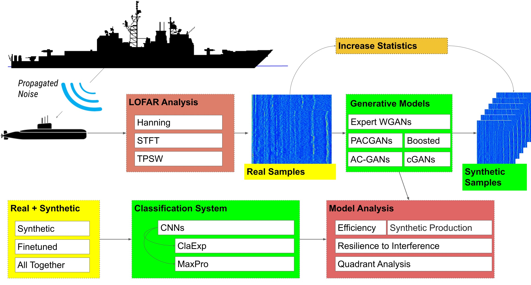
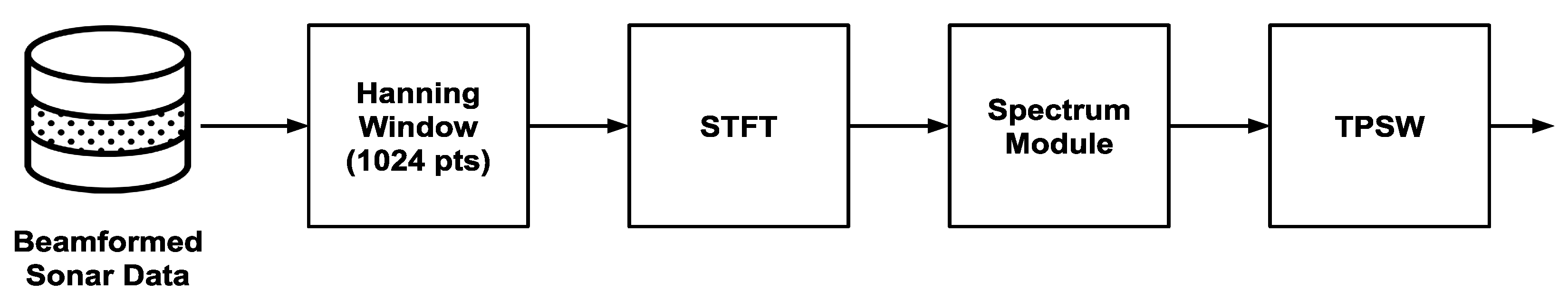
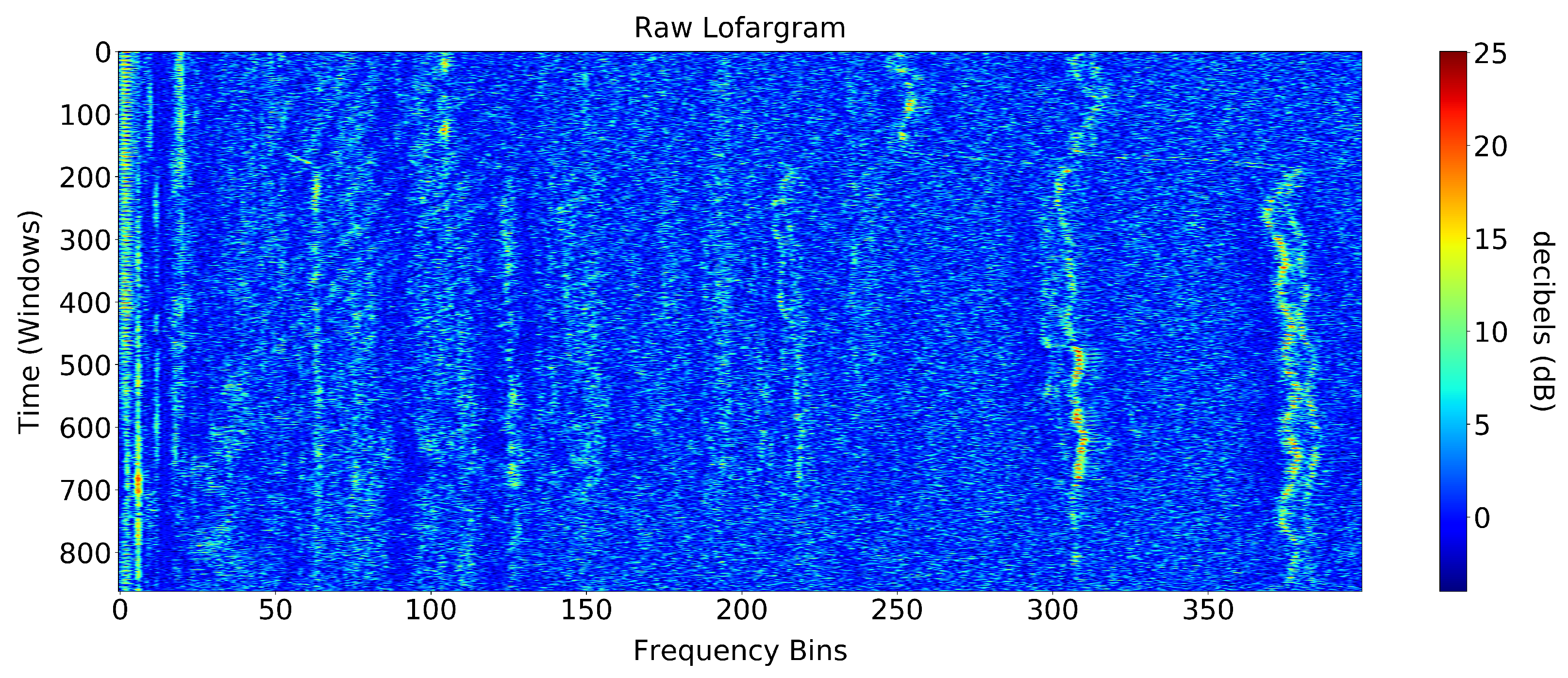
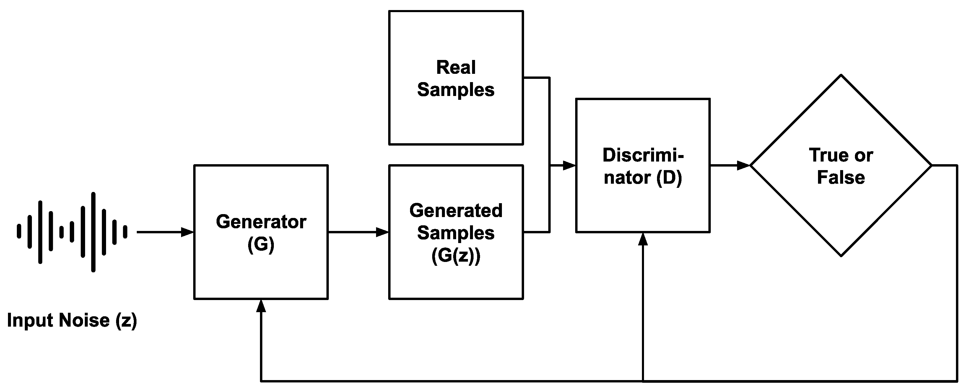
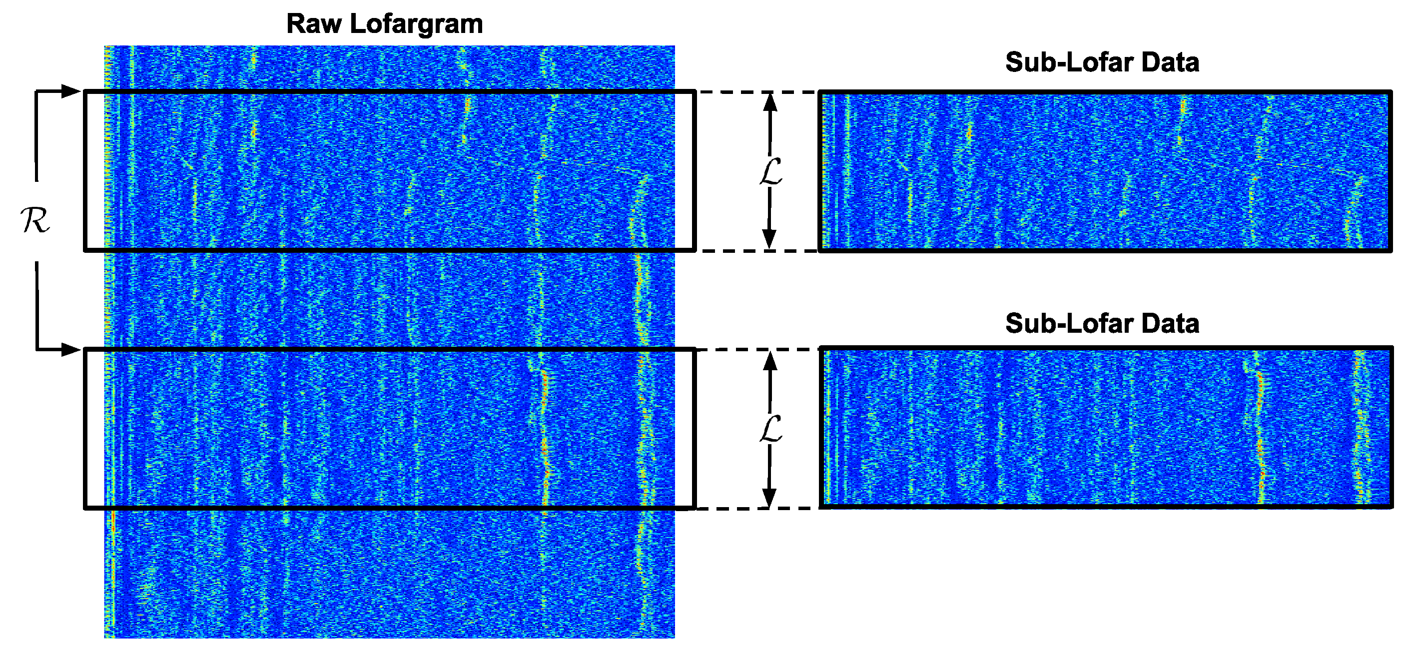
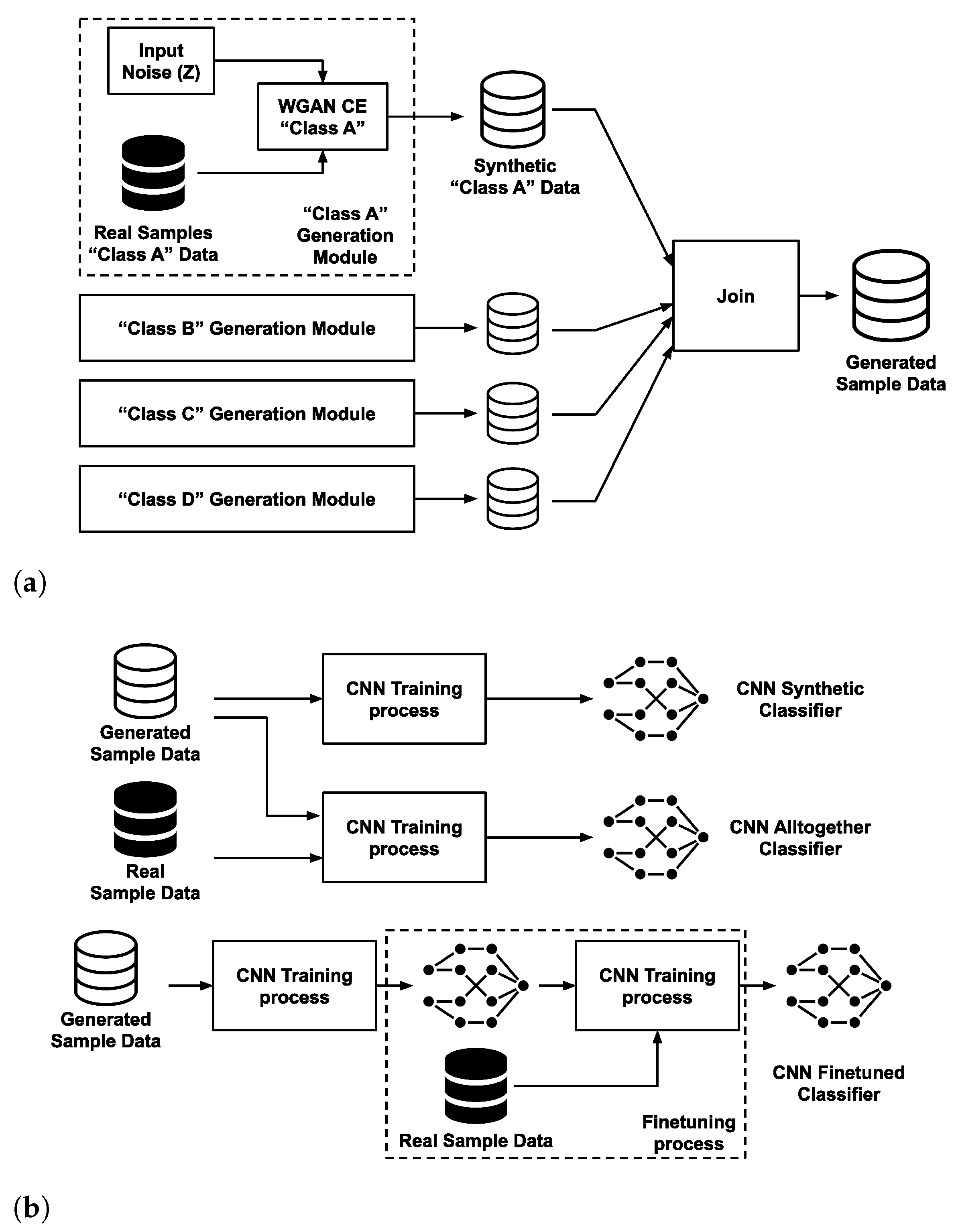
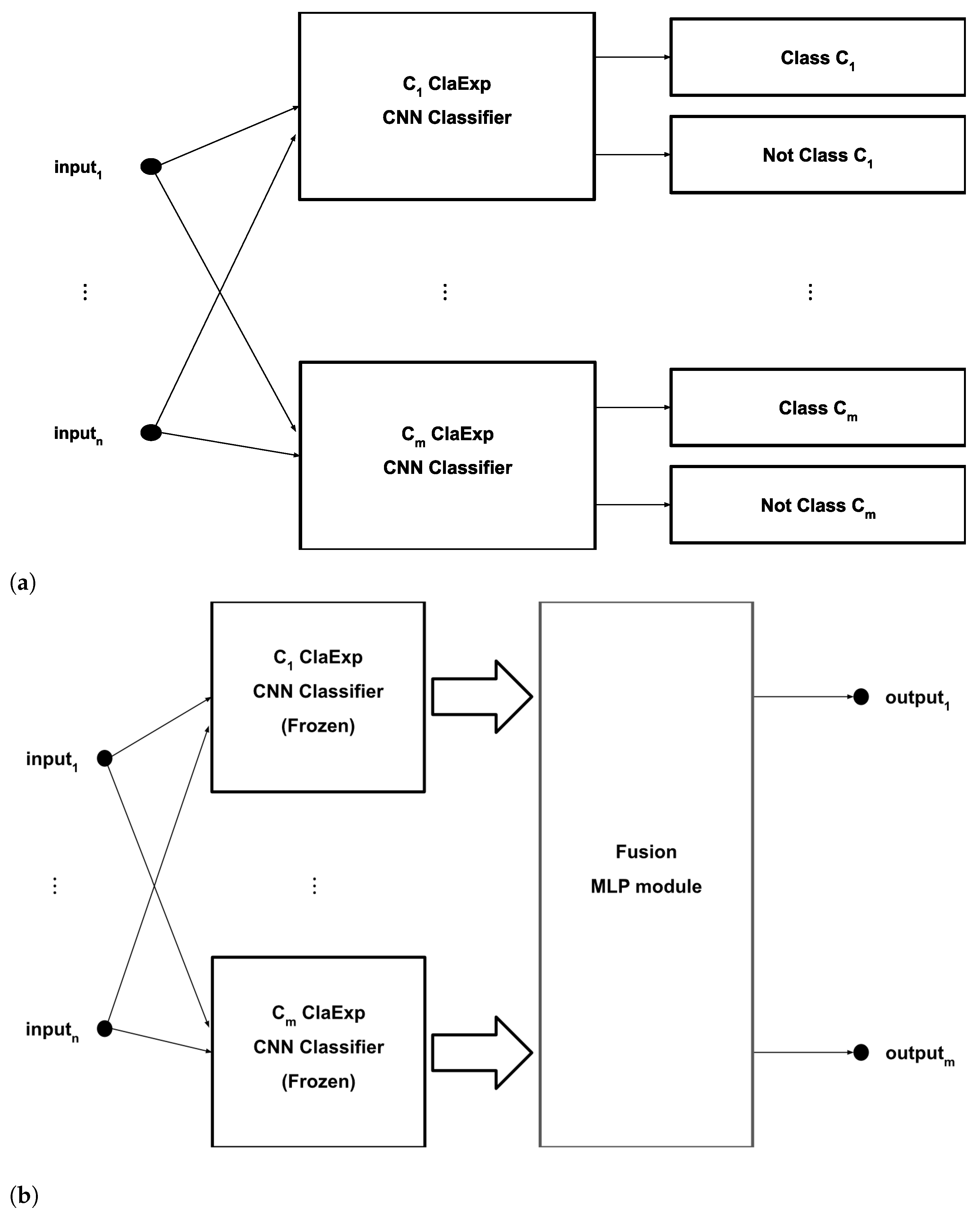
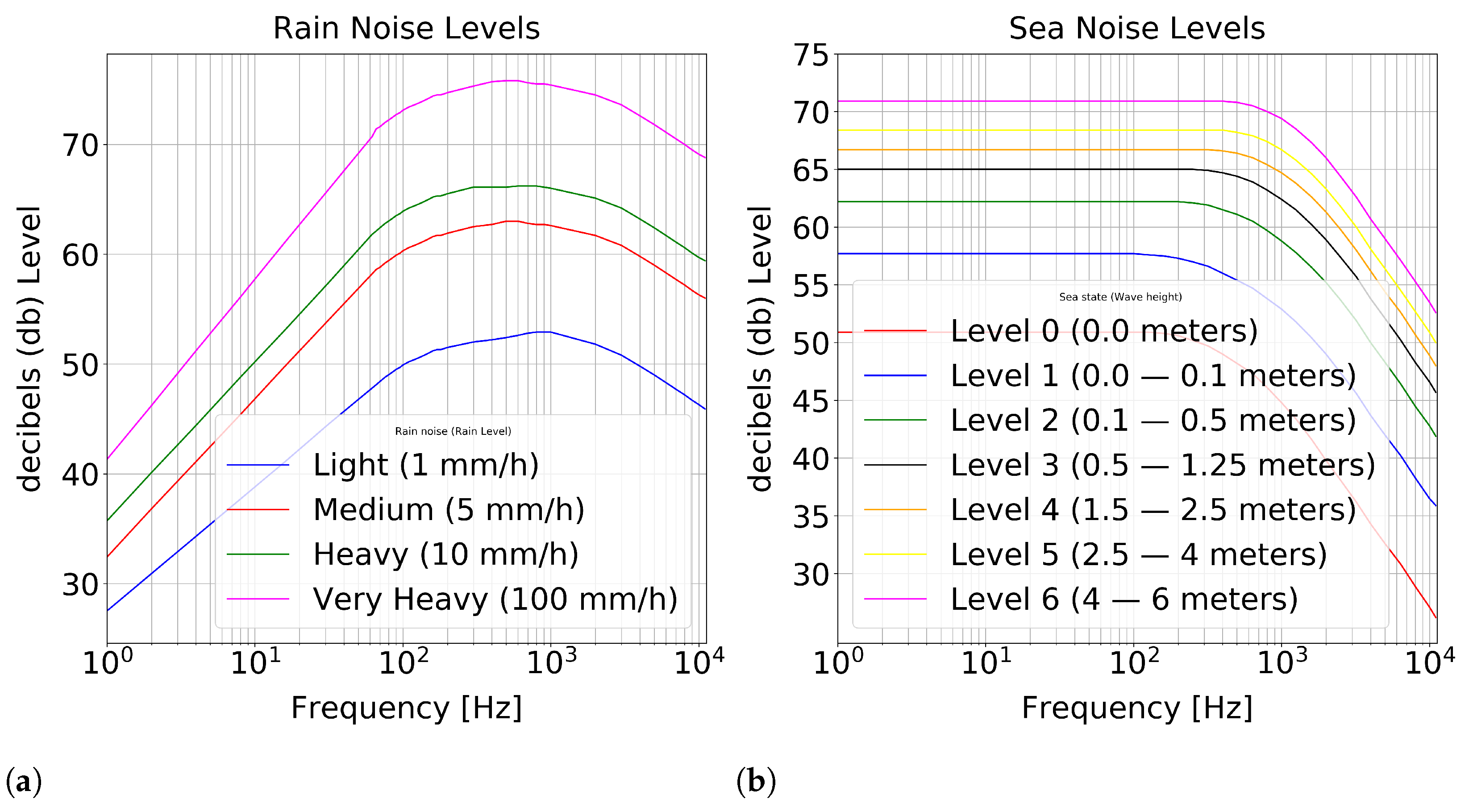
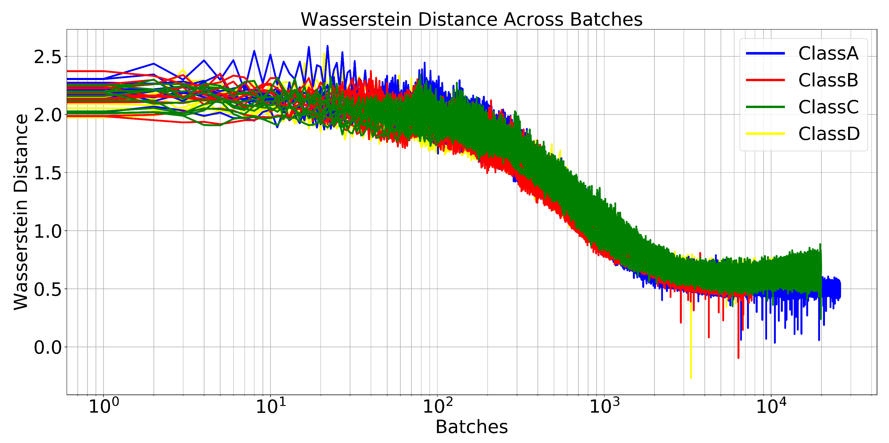
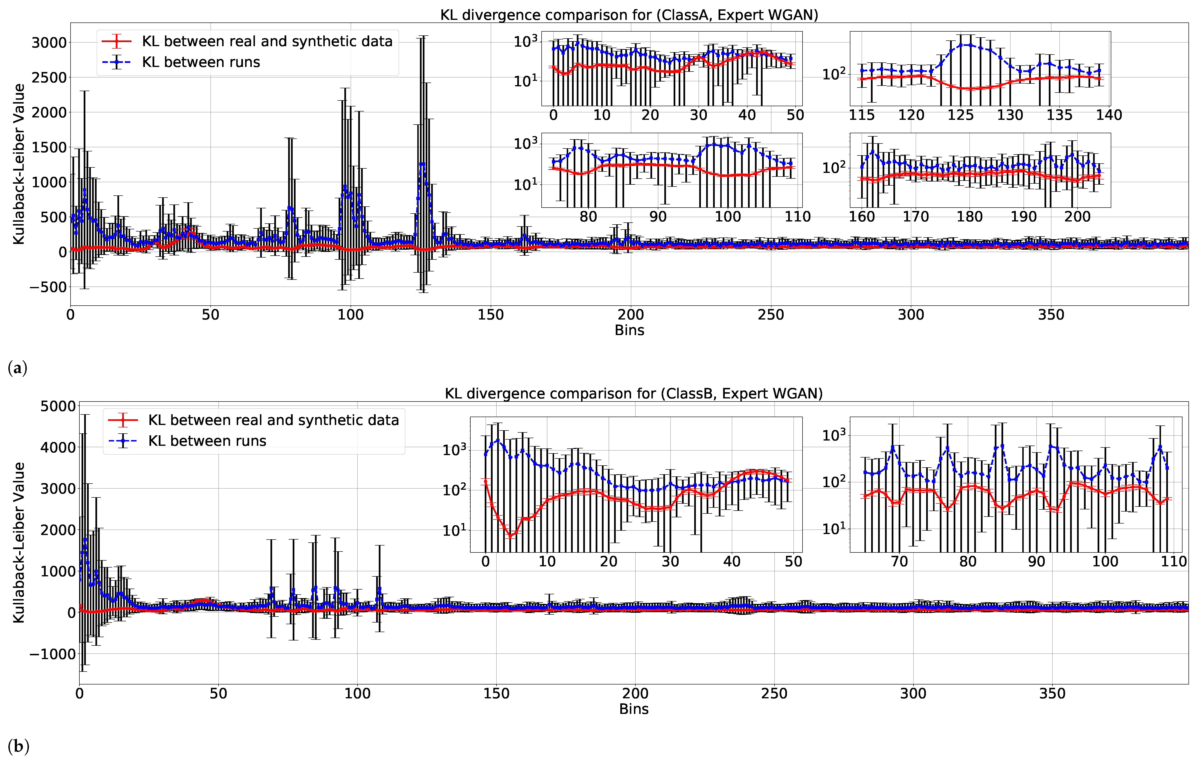
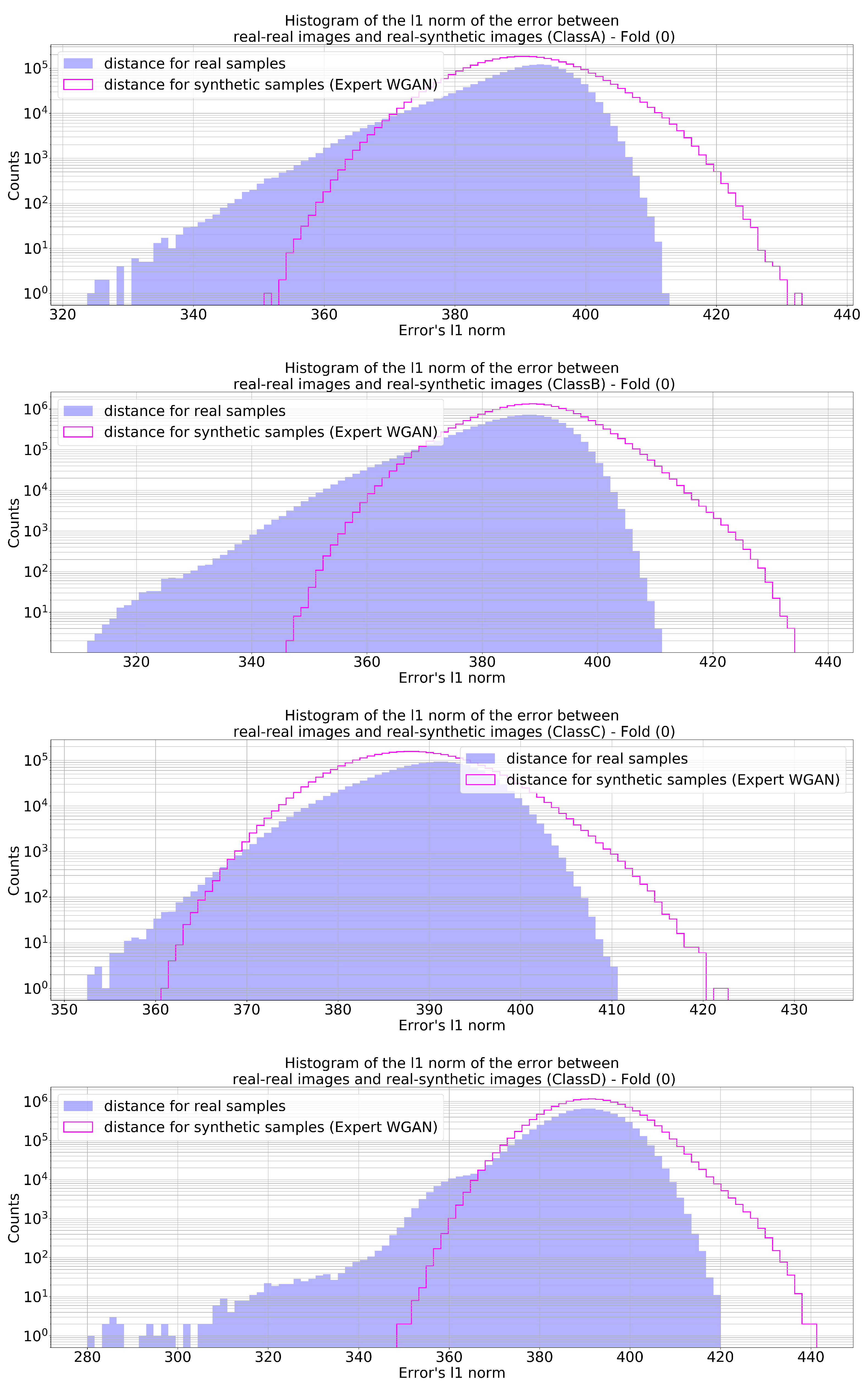
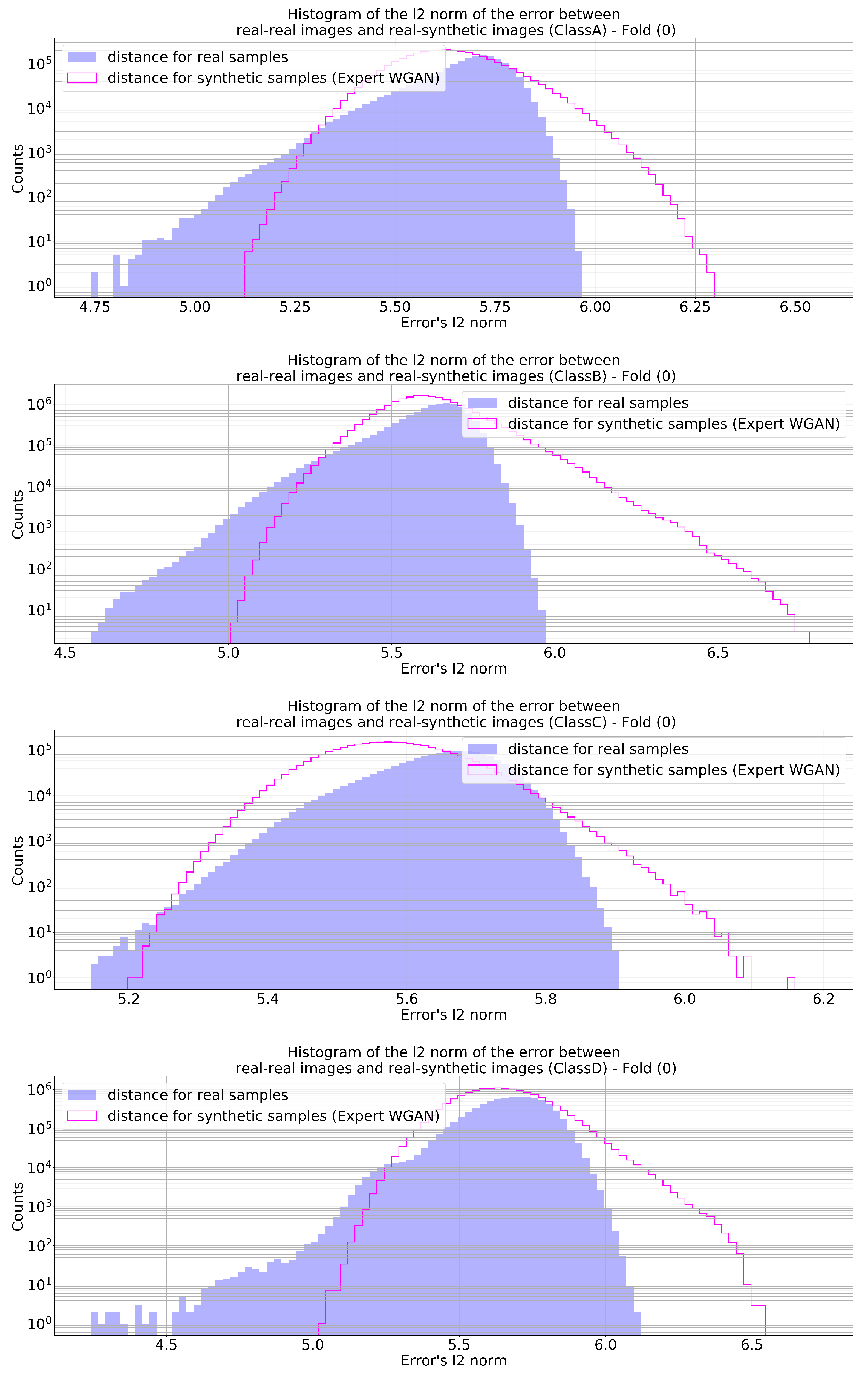
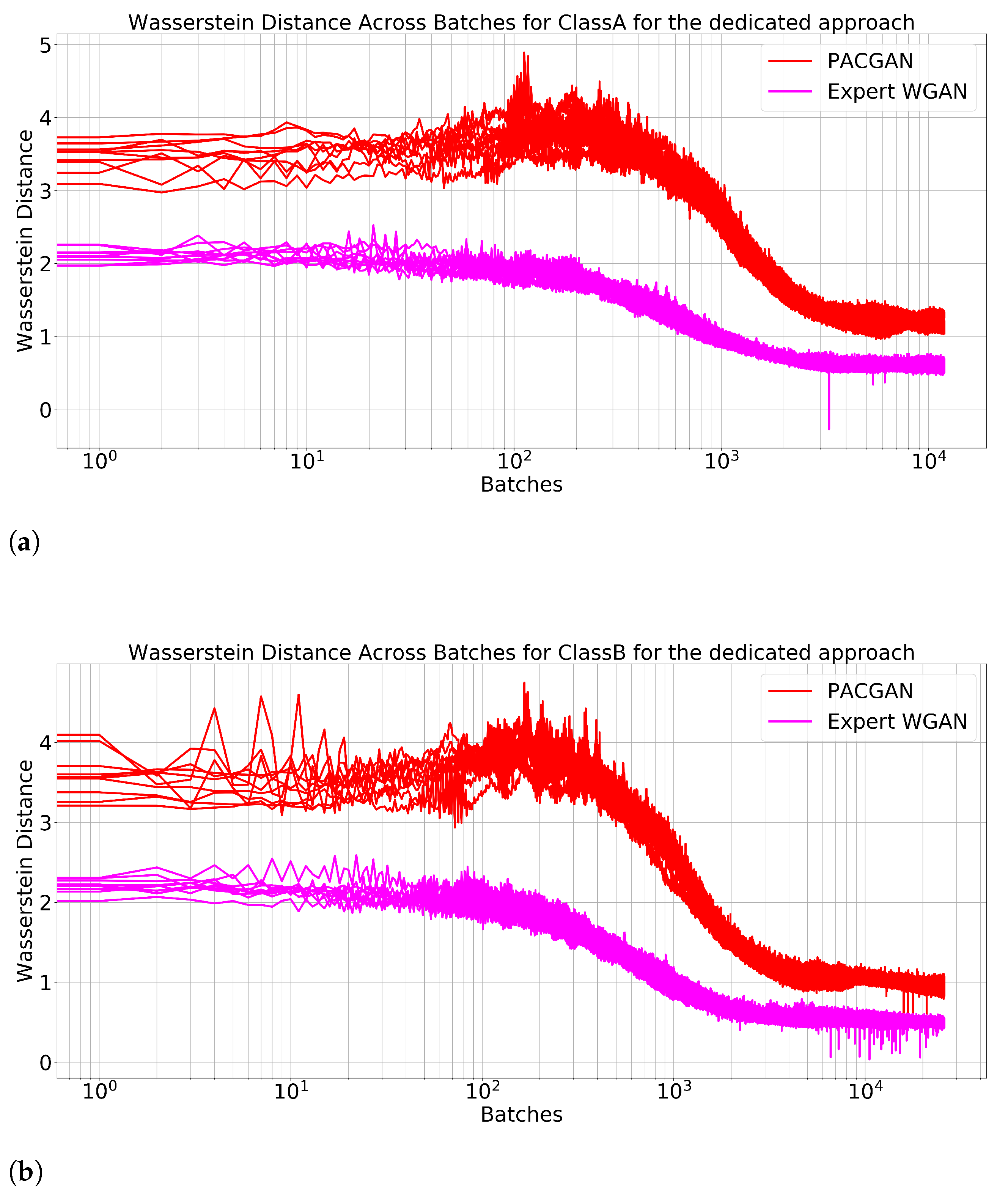
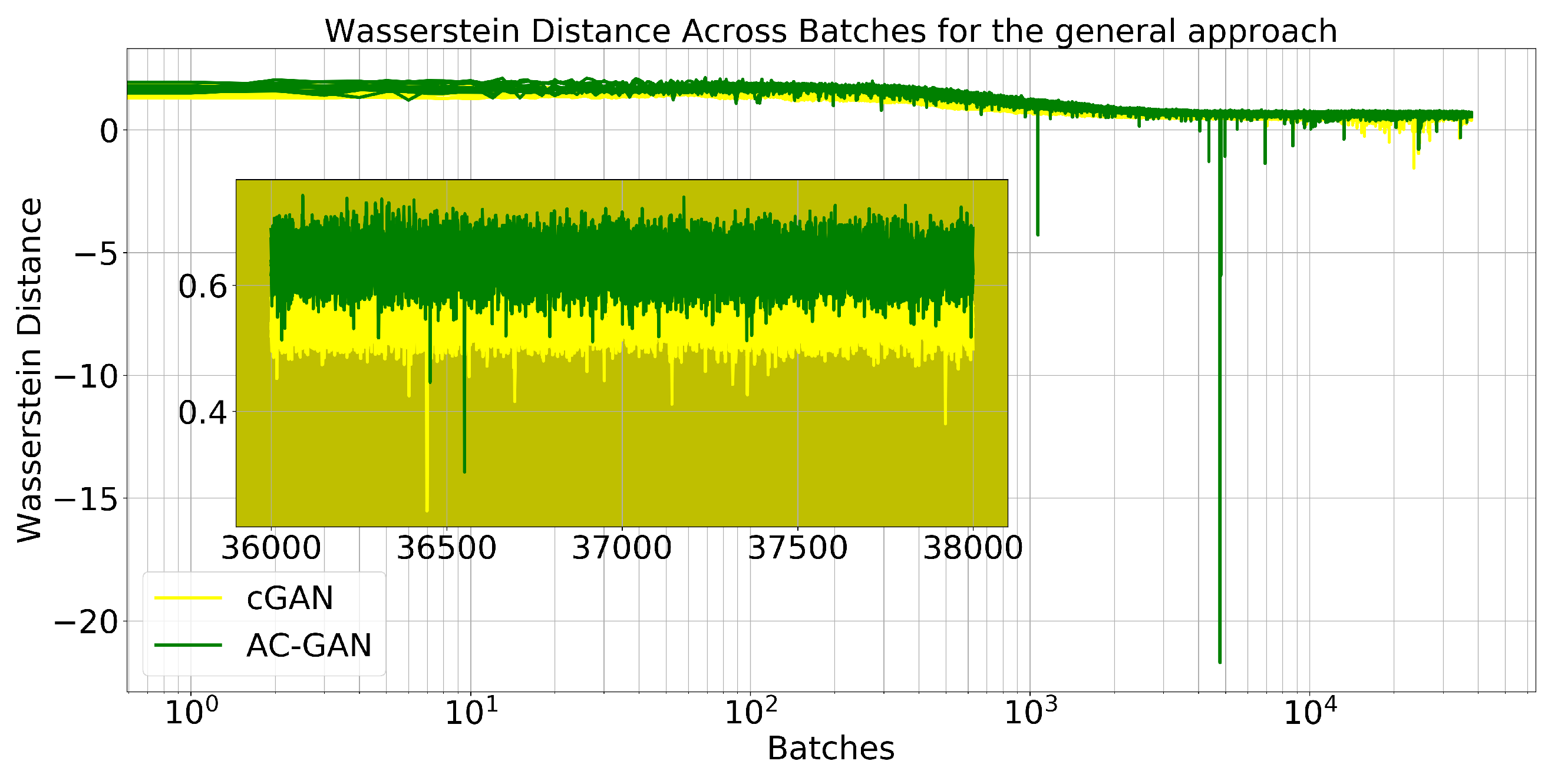
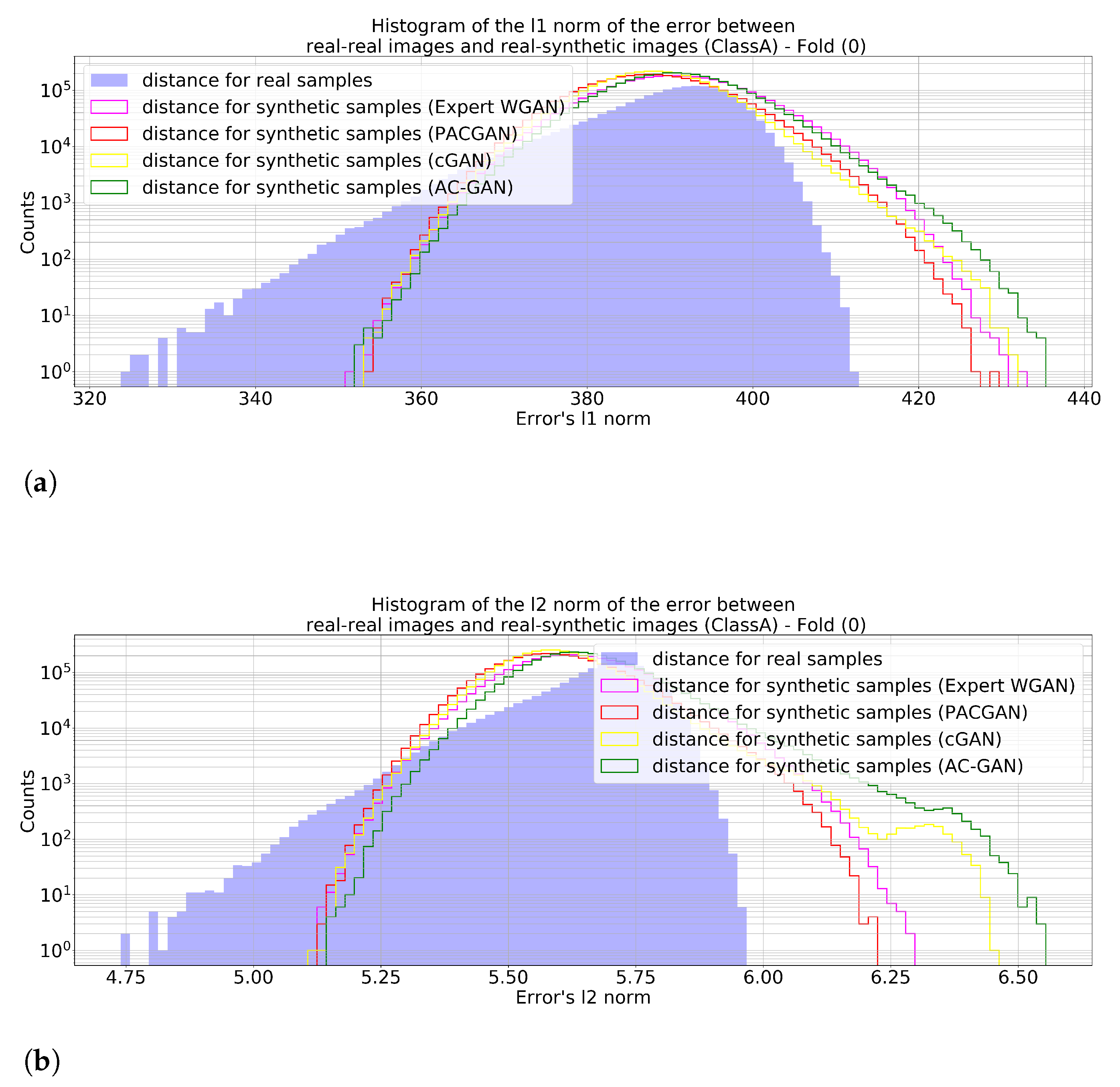
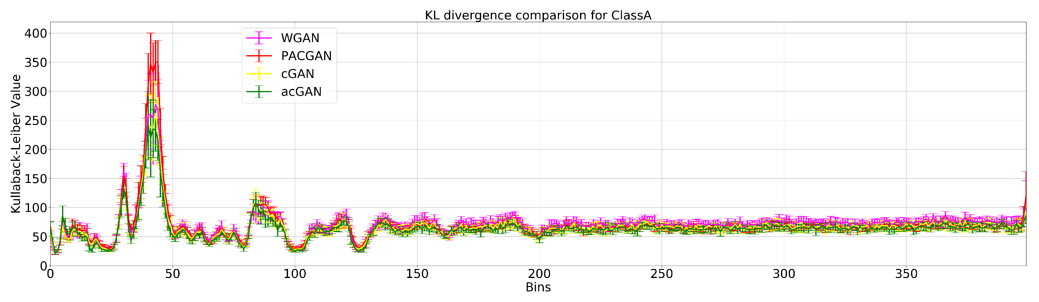
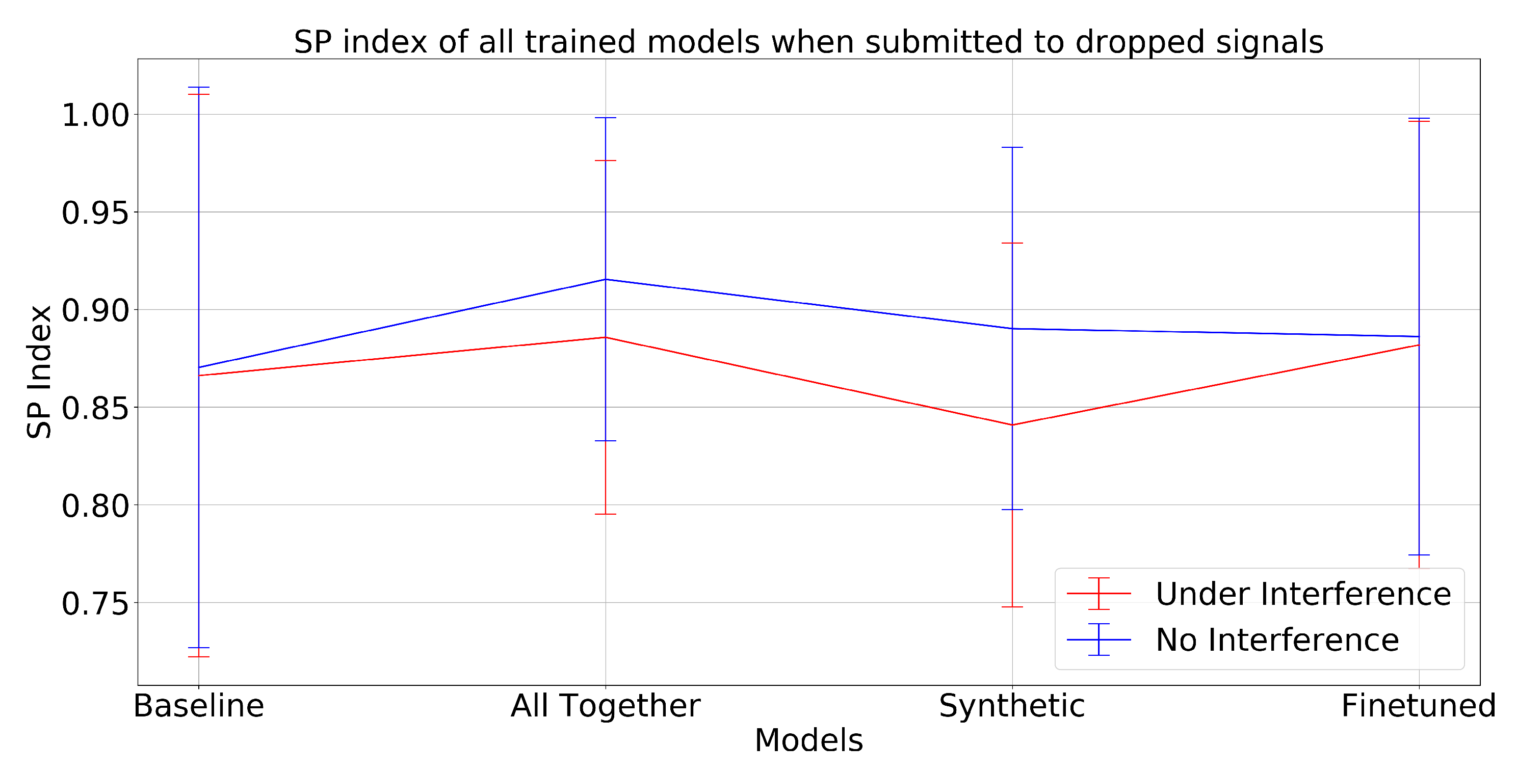
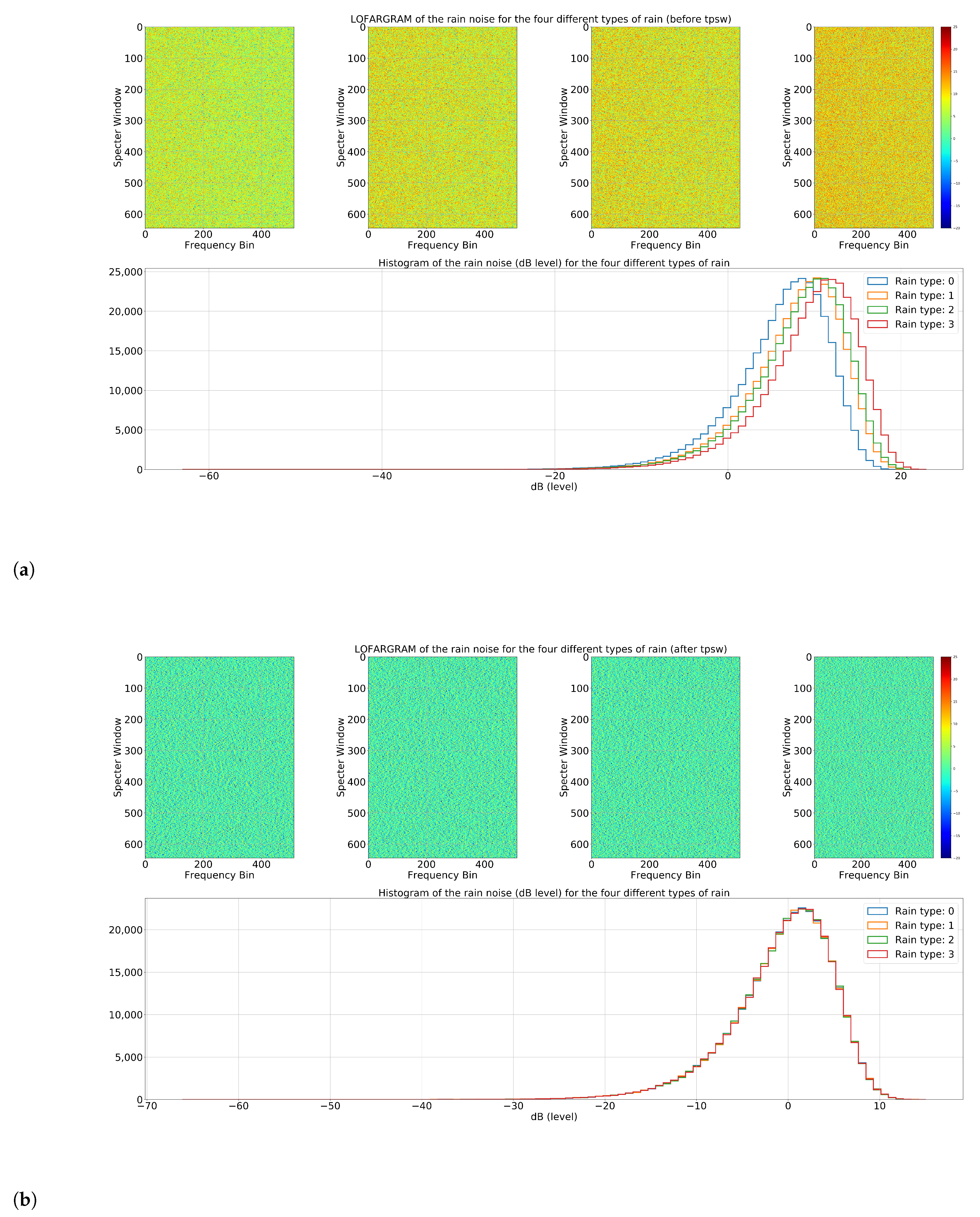
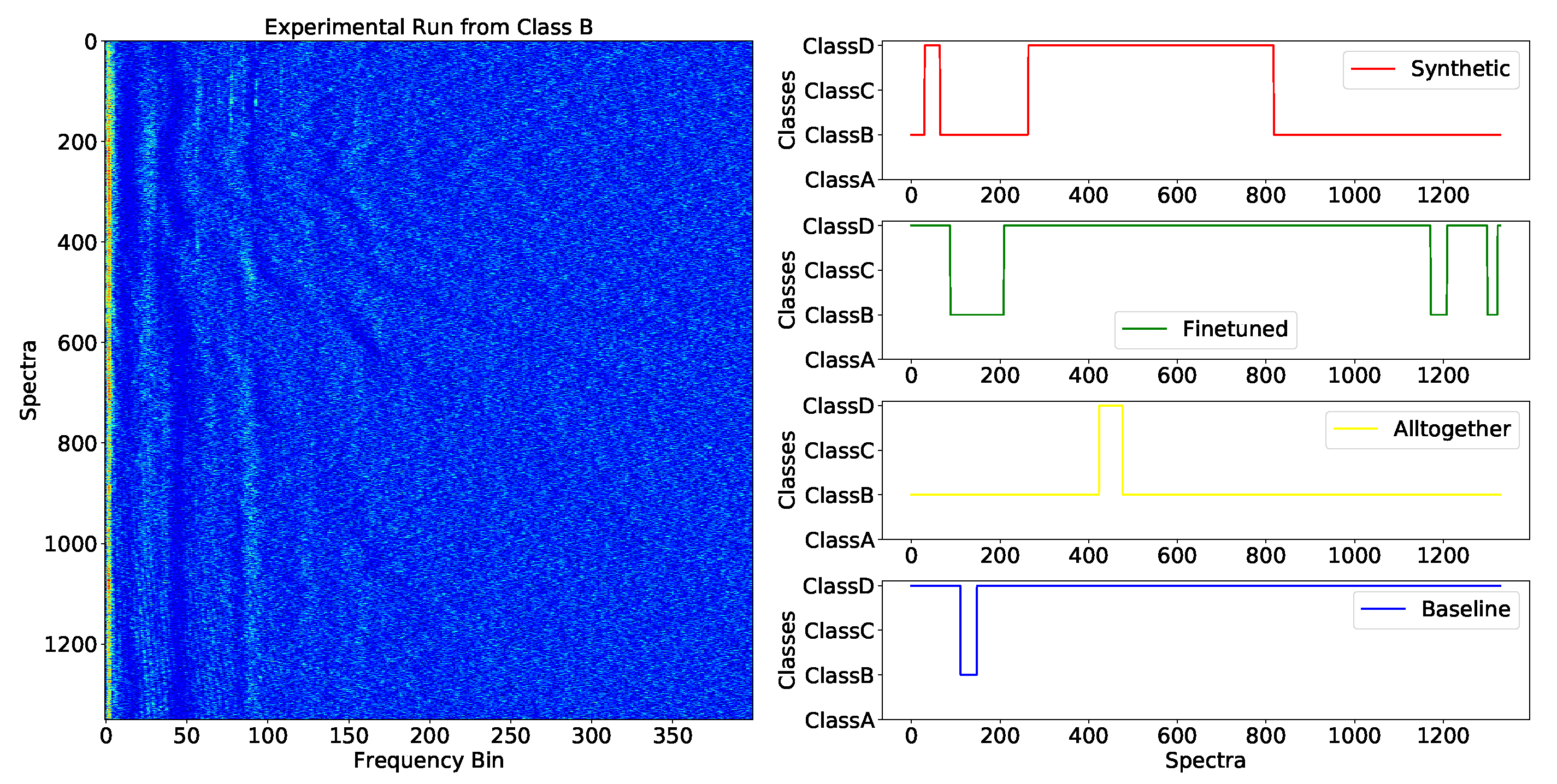
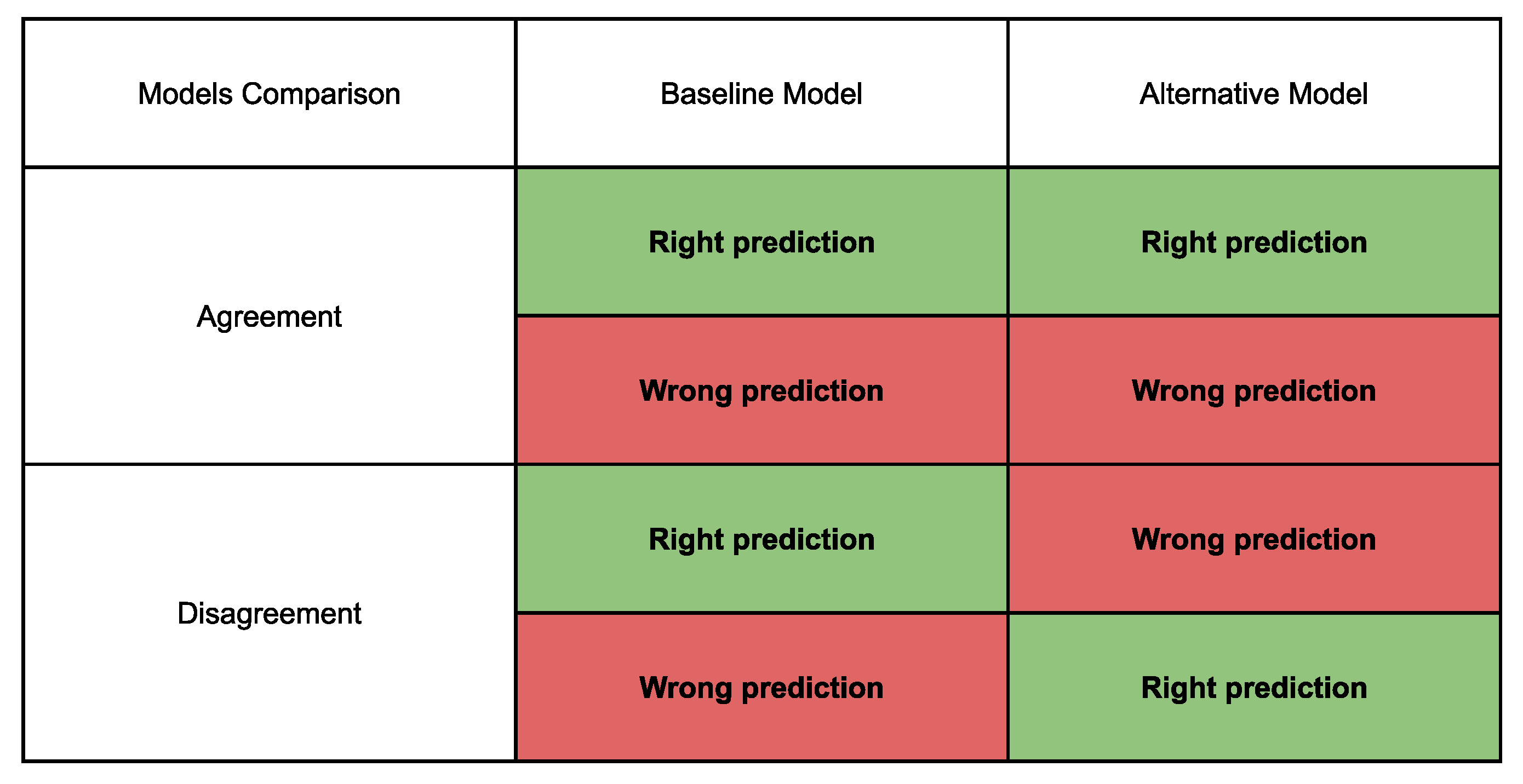
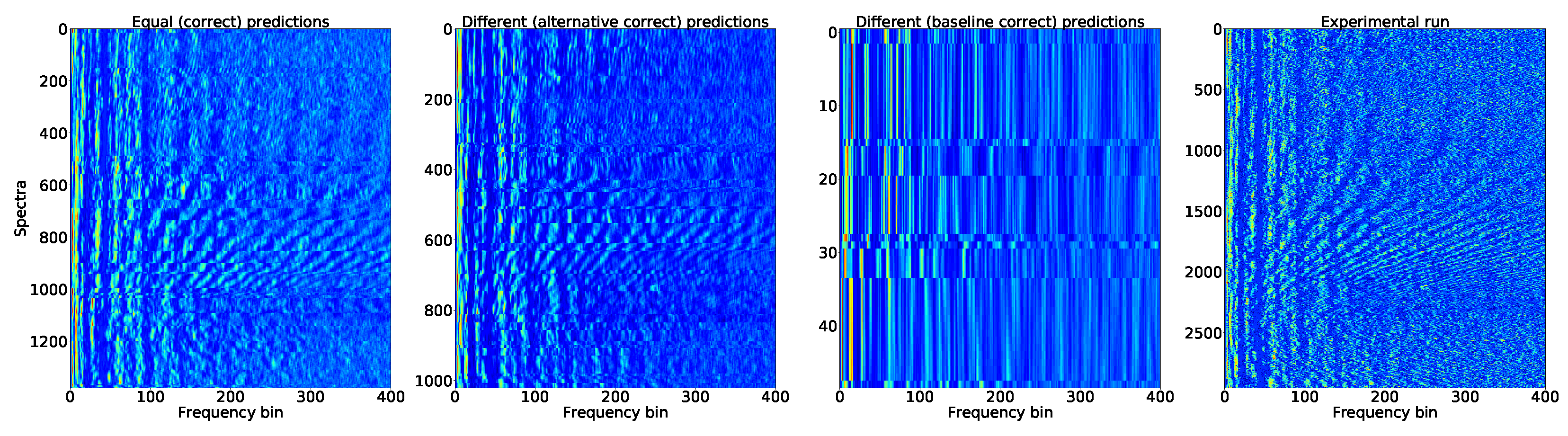
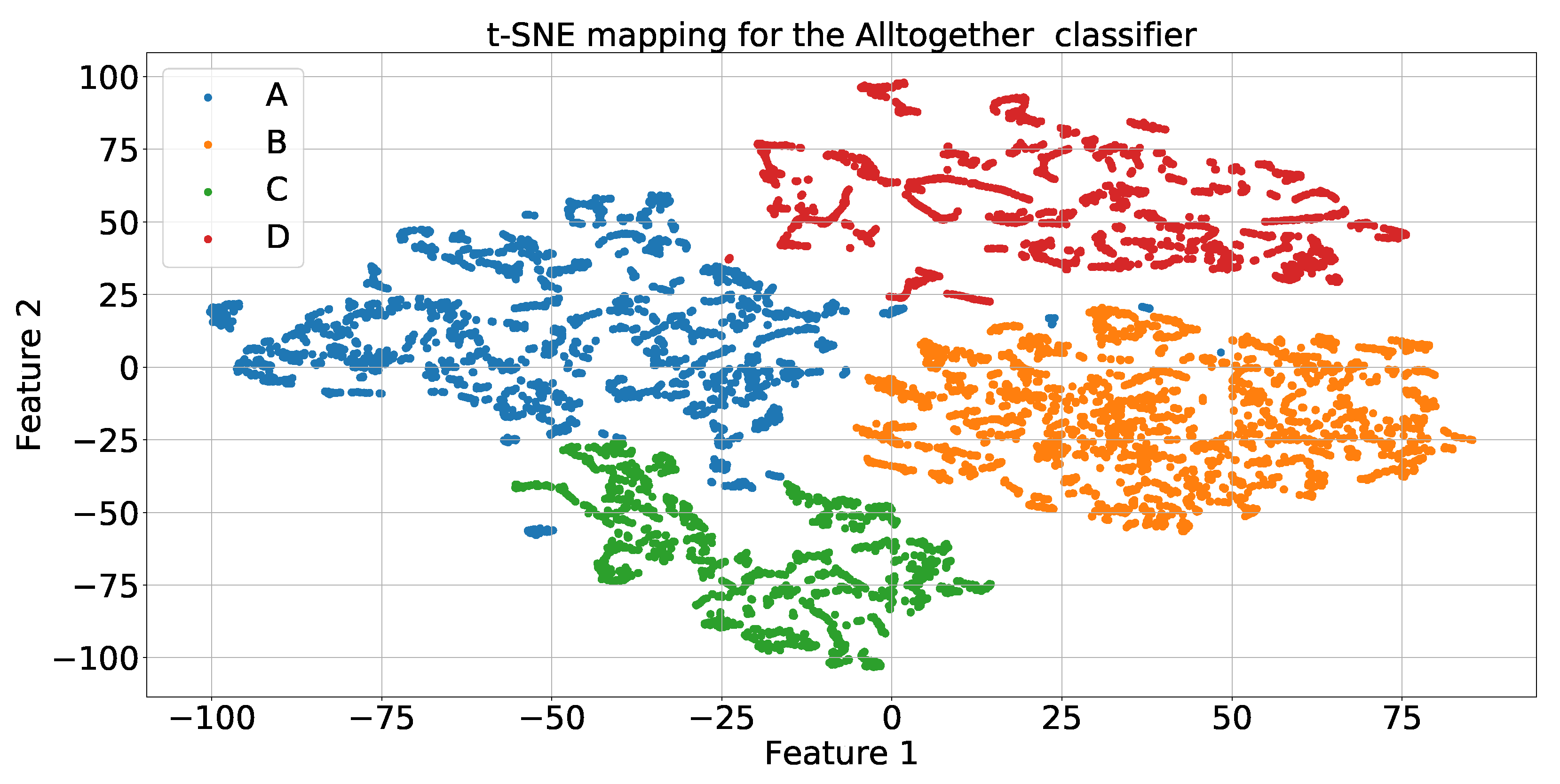
Table 1.
The dead time in data acquisition, when the number of acquisition windows required for forming the sub-images is varied.
Table 1.
The dead time in data acquisition, when the number of acquisition windows required for forming the sub-images is varied.
| 1 | 20 | 40 | 60 | 80 | 100 | 150 | |
|---|---|---|---|---|---|---|---|
| Dead Time | 0.047 s | 0.94 s | 1.88 s | 2.82 s | 3.76 s | 4.70 s | 7.05 s |
Table 2.
Amount of images that remain after the sub-imaging construction, taking all runs in Class A as an example, for several possible configurations of sub-image parameters.
Table 2.
Amount of images that remain after the sub-imaging construction, taking all runs in Class A as an example, for several possible configurations of sub-image parameters.
| 1 | 5 | 10 | 20 | 30 | 40 | 50 | 100 | |
|---|---|---|---|---|---|---|---|---|
| 5 | 2588 | 2584 | 2579 | 2569 | 2559 | 2549 | 2539 | 2489 |
| 10 | 1295 | 1294 | 1290 | 1285 | 1280 | 1275 | 1270 | 1245 |
| 20 | 649 | 648 | 646 | 644 | 641 | 639 | 636 | 624 |
| 30 | 434 | 433 | 431 | 430 | 429 | 426 | 425 | 416 |
| 40 | 325 | 325 | 325 | 324 | 321 | 320 | 320 | 314 |
| 50 | 260 | 260 | 260 | 260 | 259 | 256 | 255 | 250 |
| 100 | 130 | 130 | 130 | 130 | 130 | 130 | 130 | 125 |
Table 3.
Generative model topologies.
| Model | Layer | Type | Number of Neurons | Kernel Size | Activation | Stride | Padding |
|---|---|---|---|---|---|---|---|
| Generator | 1 | Dense | 500 | - | ReLU | - | - |
| 2 | Reshape | 5 × 100 | - | - | - | - | |
| 3 | Up-Sampling | - | - | - | 2 | - | |
| 4 | Convolutional | 128 | 5 | ReLU | 1 | SAME | |
| 5 | Up-Sampling | - | - | - | 2 | - | |
| 6 | Convolutional | 64 | 5 | ReLU | 1 | SAME | |
| 7 | Convolutional | 1 | 5 | Tanh | 1 | SAME | |
| Discriminator | 1 | Convolutional | 16 | 5 | ReLU | 1 | SAME |
| 2 | Convolutional | 32 | 5 | ReLU | 2 | SAME | |
| 3 | Convolutional | 64 | 5 | ReLU | 2 | SAME | |
| 4 | Flatten | - | - | - | - | - | |
| 5 | Dense | 50 | - | ReLU | - | - | |
| 6 | Dense | 1 | - | Linear | - | - |
Table 4.
Topology for the CNN classifiers.
| Layer | Type | Number of Neurons | Kernel Size | Activation | Stride | Padding |
|---|---|---|---|---|---|---|
| 1 | Convolutional | 16 | 5 | ReLU | 2 | SAME |
| 2 | Convolutional | 32 | 5 | ReLU | 2 | SAME |
| 3 | Dropout | - | - | - | - | - |
| 4 | Convolutional | 64 | 5 | ReLU | 2 | SAME |
| 5 | Dropout | - | - | - | - | - |
| 6 | Convolutional | 128 | 5 | ReLU | 2 | SAME |
| 7 | Dropout | - | - | - | - | - |
| 8 | Flatten | - | - | - | - | - |
| 9 | Dense | 100 | - | ReLU | - | - |
| 10 | Dense | 50 | - | ReLU | - | - |
| 11 | Dense | 4 | - | ReLU | - | - |
Table 5.
Maximum SP index and accuracy computed for several values of the L and R parameters applied to the different strategies tested.
Table 5.
Maximum SP index and accuracy computed for several values of the L and R parameters applied to the different strategies tested.
| Strategy | |||||
|---|---|---|---|---|---|
| 5 | 10 | 20 | |||
| SP | Baseline | 20 | 97.7 ± 1.3 | 97.5 ± 2.7 | 96.6 ± 3.3 |
| Synthetic | 96.0 ± 1.2 | 92.4 ± 2.5 | 87.4 ± 5.1 | ||
| Fine-tuned | 98.8 ± 0.6 | 98.4 ± 1.2 | 97.4 ± 2.0 | ||
| All together | 98.6 ± 0.5 | 98.0 ± 1.4 | 97.6 ± 1.8 | ||
| Baseline | 40 | 97.4 ± 3.5 | 97.4 ± 3.3 | 96.3 ± 3.9 | |
| Synthetic | 96.9 ± 1.7 | 95.3 ± 1.5 | 92.7 ± 2.2 | ||
| Fine-tuned | 99.0 ± 1.3 | 98.7 ± 0.9 | 98.0 ± 2.1 | ||
| All together | 98.7 ± 1.2 | 98.3 ± 1.4 | 97.4 ± 1.5 | ||
| Acc | Baseline | 20 | 98.2 ± 1.0 | 97.6 ± 2.7 | 96.9 ± 2.8 |
| Synthetic | 96.8 ± 0.8 | 94.3 ± 1.4 | 90.2 ± 3.7 | ||
| Fine-tuned | 99.0 ± 0.4 | 98.7 ± 0.7 | 97.7 ± 1.7 | ||
| All together | 98.8 ± 0.4 | 98.5 ± 1.0 | 98.0 ± 1.2 | ||
| Baseline | 40 | 97.3 ± 3.5 | 97.6 ± 3.3 | 96.4 ± 3.6 | |
| Synthetic | 97.8 ± 1.1 | 96.5 ± 1.0 | 94.7 ± 1.2 | ||
| Fine-tuned | 99.1 ± 1.0 | 98.9 ± 0.7 | 98.2 ± 1.2 | ||
| All together | 99.1 ± 0.8 | 98.7 ± 1.0 | 97.8 ± 1.2 | ||
Table 6.
Figures of merit for all design strategies measured from the window-based cross-validation method. Synthetic data generated with the expert WGAN.
Table 6.
Figures of merit for all design strategies measured from the window-based cross-validation method. Synthetic data generated with the expert WGAN.
| Training Paradigm | Strategy | Accuracy | Precision | F1 | Recall | SP |
|---|---|---|---|---|---|---|
| MaxPro | Baseline | 98.2 ± 1.0 | 97.7 ± 1.2 | 97.7 ± 1.2 | 97.8 ± 1.3 | 97.7 ± 1.3 |
| Synthetic | 96.8 ± 0.8 | 96.3 ± 1.1 | 96.1 ± 1.0 | 96.1 ± 1.2 | 96.0 ± 1.2 | |
| Fine-tuned | 99.0 ± 0.4 | 98.7 ± 0.6 | 98.7 ± 0.6 | 98.8 ± 0.6 | 98.8 ± 0.6 | |
| All together | 98.8 ± 0.4 | 98.4 ± 0.6 | 98.5 ± 0.5 | 98.6 ± 0.5 | 98.6 ± 0.5 | |
| ClaExp | Baseline | 98.8 ± 0.8 | 98.4 ± 1.0 | 98.4 ± 1.0 | 98.5 ± 1.1 | 98.5 ± 1.1 |
| Synthetic | 97.8 ± 0.5 | 97.4 ± 0.7 | 97.3 ± 0.7 | 97.2 ± 0.8 | 97.2 ± 0.8 | |
| Fine-tuned | 99.0 ± 0.8 | 98.7 ± 1.1 | 98.7 ± 1.0 | 98.8 ± 1.0 | 98.8 ± 1.0 | |
| All together | 99.0 ± 0.6 | 98.7 ± 0.7 | 98.6 ± 0.8 | 98.6 ± 1.0 | 98.6 ± 1.0 |
Table 7.
Figures of merit for all design strategies measured from the LORO cross-validation method. Synthetic data generated with the expert WGAN.
Table 7.
Figures of merit for all design strategies measured from the LORO cross-validation method. Synthetic data generated with the expert WGAN.
| Training Paradigm | Strategy | Accuracy | Precision | F1 | Recall | SP |
|---|---|---|---|---|---|---|
| MaxPro | Baseline | 89.4 ± 11.0 | 89.5 ± 10.8 | 87.2 ± 13.8 | 89.4 ± 11.0 | 87.0 ± 14.3 |
| Synthetic | 90.2 ± 8.5 | 90.5 ± 8.0 | 88.7 ± 9.8 | 90.0 ± 8.0 | 89.0 ± 9.3 | |
| Fine-tuned | 90.3 ± 9.5 | 90.8 ± 9.0 | 88.6 ± 11.5 | 90.3 ± 9.1 | 88.7 ± 11.2 | |
| All together | 92.4 ± 7.3 | 92.7 ± 6.6 | 91.2 ± 8.9 | 92.5 ± 6.6 | 91.5 ± 8.3 | |
| ClaExp | Baseline | 88.3 ± 11.7 | 89.3 ± 10.5 | 86.2 ± 14.0 | 88.0 ± 11.8 | 85.9 ± 14.6 |
| Synthetic | 89.9 ± 9.4 | 91.4 ± 7.1 | 88.0 ± 11.6 | 90.0 ± 8.1 | 87.8 ± 11.6 | |
| Fine-tuned | 90.9 ± 9.6 | 91.5 ± 8.6 | 89.0 ± 12.4 | 91.0 ± 8.8 | 88.4 ± 13.8 | |
| All together | 90.4 ± 8.4 | 91.7 ± 6.9 | 88.6 ± 9.8 | 89.7 ± 7.0 | 88.2 ± 9.4 |
Table 8.
Figures of merit for all design strategies measured from the window-based and LORO cross-validation methods for the MaxPro approach. Synthetic data generated with the cGAN.
Table 8.
Figures of merit for all design strategies measured from the window-based and LORO cross-validation methods for the MaxPro approach. Synthetic data generated with the cGAN.
| Cross-Validation Method | Strategy | Accuracy | Precision | F1 | Recall | SP |
|---|---|---|---|---|---|---|
| Window | Baseline | 98.2 ± 1.0 | 97.7 ± 1.2 | 97.7 ± 1.2 | 97.8 ± 1.3 | 97.7 ± 1.3 |
| Synthetic | 96.5 ± 1.3 | 95.9 ± 1.5 | 95.9 ± 1.5 | 96.1 ± 1.4 | 96.1 ± 1.5 | |
| Fine-tuned | 98.7 ± 0.8 | 98.3 ± 1.1 | 98.4 ± 1.1 | 98.5 ± 1.1 | 98.4 ± 1.1 | |
| All together | 98.0 ± 1.1 | 97.4 ± 1.5 | 97.6 ± 1.4 | 97.8 ± 1.3 | 97.8 ± 1.3 | |
| LORO | Baseline | 89.4 ± 11.0 | 89.5 ± 10.8 | 87.2 ± 13.8 | 89.4 ± 11.0 | 87.0 ± 14.3 |
| Synthetic | 90.4 ± 9.6 | 90.6 ± 8.5 | 88.5 ± 11.9 | 90.2 ± 9.5 | 88.4 ± 12.2 | |
| Fine-tuned | 91.2 ± 9.3 | 92.1 ± 7.8 | 89.6 ± 11.5 | 91.6 ± 8.4 | 89.9 ± 11.2 | |
| All together | 90.6 ± 10.1 | 90.8 ± 9.7 | 88.9 ± 12.3 | 90.6 ± 9.3 | 88.8 ± 12.5 |
Table 9.
Figures of merit measured from the window-based and LORO cross-validation methods for the MaxPro approach. Calculated using the auxiliary classifier of the AC-GAN.
Table 9.
Figures of merit measured from the window-based and LORO cross-validation methods for the MaxPro approach. Calculated using the auxiliary classifier of the AC-GAN.
| Cross-Validation Method | Strategy | Accuracy | Recall | F1 | SP |
|---|---|---|---|---|---|
| Window | Baseline | 98.2 ± 1.0 | 97.8 ± 1.3 | 97.7 ± 1.2 | 97.7 ± 1.3 |
| Auxiliary | 94.6 ± 1.7 | 94.1 ± 1.6 | 93.8 ± 1.8 | 94.1 ± 1.6 | |
| LORO | Baseline | 89.4 ± 11.0 | 89.4 ± 11.0 | 87.2 ± 13.8 | 87.0 ± 14.3 |
| Auxiliary | 89.4 ± 11.2 | 89.6 ± 10.5 | 88.1 ± 12.9 | 88.5 ± 12.4 |
Publisher’s Note: MDPI stays neutral with regard to jurisdictional claims in published maps and institutional affiliations. |
© 2022 by the authors. Licensee MDPI, Basel, Switzerland. This article is an open access article distributed under the terms and conditions of the Creative Commons Attribution (CC BY) license (https://creativecommons.org/licenses/by/4.0/).
Share and Cite
MDPI and ACS Style
Fernandes, J.d.C.V.; de Moura Junior, N.N.; de Seixas, J.M. Deep Learning Models for Passive Sonar Signal Classification of Military Data. Remote Sens. 2022, 14, 2648. https://0-doi-org.brum.beds.ac.uk/10.3390/rs14112648
AMA Style
Fernandes JdCV, de Moura Junior NN, de Seixas JM. Deep Learning Models for Passive Sonar Signal Classification of Military Data. Remote Sensing. 2022; 14(11):2648. https://0-doi-org.brum.beds.ac.uk/10.3390/rs14112648
Chicago/Turabian StyleFernandes, Júlio de Castro Vargas, Natanael Nunes de Moura Junior, and José Manoel de Seixas. 2022. "Deep Learning Models for Passive Sonar Signal Classification of Military Data" Remote Sensing 14, no. 11: 2648. https://0-doi-org.brum.beds.ac.uk/10.3390/rs14112648
Note that from the first issue of 2016, this journal uses article numbers instead of page numbers. See further details here.