
Densely Residual Network with Dual Attention for Hyperspectral Reconstruction from RGB Images


1
Xiaomi, Nanjing 210019, China
2
Department of Computer Science, Faculty of Information Technology and Electrical Engineering, Norwegian University of Science and Technology, N-2815 Gjøvik, Norway
*
Author to whom correspondence should be addressed.
Remote Sens. 2022, 14(13), 3128; https://0-doi-org.brum.beds.ac.uk/10.3390/rs14133128
Submission received: 5 March 2022
/
Revised: 7 June 2022
/
Accepted: 10 June 2022
/
Published: 29 June 2022
(This article belongs to the Special Issue Machine Learning for Remote Sensing Image/Signal Processing)
Abstract
:In the last several years, deep learning has been introduced to recover a hyperspectral image (HSI) from a single RGB image and demonstrated good performance. In particular, attention mechanisms have further strengthened discriminative features, but most of them are learned by convolutions with limited receptive fields or require much computational cost, which hinders the function of attention modules. Furthermore, the performance of these deep learning methods is hampered by tackling multi-level features equally. To this end, in this paper, based on multiple lightweight densely residual modules, we propose a densely residual network with dual attention (DRN-DA), which utilizes advanced attention and adaptive fusion strategy for more efficient feature correlation learning and more powerful feature extraction. Specifically, an SE layer is applied to learn channel-wise dependencies, and dual downsampling spatial attention (DDSA) is developed to capture long-range spatial contextual information. All the intermediate-layer feature maps are adaptively fused. Experimental results on four data sets from the NTIRE 2018 and NTIRE 2020 Spectral Reconstruction Challenges demonstrate the superiority of the proposed DRN-DA over state-of-the-art methods (at least −6.19% and −1.43% on NTIRE 2018 “Clean” track and “Real World” track, −6.85% and −5.30% on NTIRE 2020 “Clean” track and “Real World” track) in terms of mean relative absolute error.
1. Introduction
With the increasing applications of computer vision technology in various engineering fields [1,2,3,4,5,6,7,8,9,10,11], hyperspectral images (HSIs) have proved to obtain more helpful information than RGB images. Hyperspectral images contain the reflectance of objects or scenes in different spectral bands, usually ranging from several dozens to hundreds, even outside the visible spectrum (e.g., in the ultraviolet or infrared spectrum). Compared with traditional RGB images with increased spectral range and resolution, HSIs provide much richer information, which has been widely used in cultural heritage [1,2], medical diagnosis [3], remote sensing [4], food quality inspection [5], color quality control [6], and various computer vision tasks, such as face recognition, object tracking, and image classification [7,8,9].
Due to the growing need for HSIs, various hyperspectral imaging systems (HISs) have been developed in the last several decades. The first HISs, such as NASA’s airborne visible/infrared imaging spectrometer (AVIRIS) [12], employed a prism to disperse the reflected light and a linear array detector to record the reflected light. This kind of HISs can acquire images with high spatial/spectral resolution in “whisk broom” imaging mode, but image acquisition is time-consuming since they adopt the point-scanning method. Afterwards, “push broom” HISs, such as NASA’s advanced land imager (ALI) [13], and “staring” HISs, often used in microscopy or other lab applications, have been developed. With a scan lens and an entrance slit, “push broom” HISs use a prism-grating-prism to split the light and can scan one line at a time; “staring” HISs use continuously changeable narrow bandpass filters in front of a matrix detector and can capture the image at one wavelength at a given time. Obviously, the latter two have relatively fast speed of scanning, but their temporal resolutions are still not high enough for dynamic scenes. Thus, many non-scanning, snapshot HISs have been designed, including computed tomographic imaging spectrometry (CTIS), fiber-reformatting imaging spectrometry (FRIS), and coded aperture snapshot spectral imaging (CASSI) [14]. Unfortunately, as the total number of voxels cannot exceed the total number of pixels on the CCD camera, these HISs involve a trade-off between spatial and spectral resolution [15].
As aforementioned, HISs to directly acquire HSIs have disadvantages either in temporal resolution or in spatial resolution. In recent years, hyperspectral reconstruction from RGB images has become a very active research topic. A large number of methods have been proposed to reconstruct hyperspectral information using only RGB cameras [16,17,18,19,20,21,22,23,24,25,26,27,28,29,30,31,32,33]. In general, these methods fall into three branches: traditional, machine learning, and deep learning methods. Traditional methods include classical methods on the basis of Wiener estimation, pseudo-inverse estimation, or principal component analysis, and their various modifications, such as adaptive Wiener estimation [16], regularized local linear models [17], sequential weighted nonlinear regression models [18], and so on. Classical methods are simple and straight but not very accurate. Modified methods tend to adaptively select or weigh training samples, which enhances hyperspectral reconstruction accuracy, but are not portable and can be time-consuming. Therefore, it is hard for these traditional methods to be applied in real tasks. Fortunately, machine learning-based methods compute hyperspectral data, which makes acquisition of spectral data fast. Shallow learning models such as RBF networks [19,20], dictionary learning-based sparse coding [21,22], and manifold-based mapping [23] are typical machine learning-based methods. Nevertheless, the expression capacity of handcrafted prior models learned by these methods is so limited that the reconstructed spectra are not very accurate. In recent years, deep learning methods have been used for hyperspectral reconstruction and have achieved remarkable success. Compared to machine learning methods, deep learning methods are capable of automatically extracting high-level features and have a better generalization ability. Convolutional neural networks (CNNs) [24,25,26,27,28,29,30,31] and generative adversarial networks (GANs) [32,33] have been developed for hyperspectral reconstruction.
Though considerable progress has been made for hyperspectral reconstruction, challenges remain in deep learning-based models as noted below: (1) when using dense skip connections, the feature of each layer is propagated into all subsequent layers, resulting in a very wide network at the cost of reducing the depth of the network [34]; (2) the commonly used non-local spatial attention involves big matrix multiplications, raising the cost of computation and memory requirement, thus hindering the frequent application in the network [35]; (3) deep learning-based models for hyperspectral reconstruction neglect that the importance of different intermediate layers varies. To address these issues, we propose a densely residual network with dual attention (DRN-DA) for more powerful feature representation, which adequately enjoys the benefits of both the residual block [36] and the dense block [34]. In our proposed DRN-DA network, the basic building blocks are densely residual block (DRB) and densely residual attention block (DRAB). The difference between DRB and DRAB is that DRAB has channel attention (CA) and dual downsampling spatial attention (DDSA) to capture channel-wise and long-range spatial dependencies. Then, to reuse the features, the output features of DRB and DRAB are adaptively fused. Additionally, an adaptive multi-scale block (AMB) with larger receptive fields is used to process the features generated by the previous network. Extensive experiments demonstrate that the proposed DRN-DA network performs better when compared to the state-of-the-art methods.
In summary, the contributions of this paper are as follows:
- We propose a novel model, named densely residual network with dual attention (DRN-DA), which enhances the representation ability of feature learning for hyperspectral reconstruction.
- We propose a lightweight dense skip connection, where each layer is connected to the next layer rather than all the subsequent layers. Although this block is different from the classic DenseNet [34], it also reuses features and eliminates gradient vanishing.
- We propose a simple but effective non-local block named dual downsampling spatial attention (DDSA) to decrease the computation and memory consumption of the standard non-local block, which makes it feasible to insert multiple non-local blocks in the network for enhancing the performance.
- To further improve the learning ability of the network, we introduce an adaptive fusion block (AFB) to adaptively reuse the features from different intermediate layers.
2. Related Works
2.1. Hyperspectral Reconstruction with Deep Learning Methods
Many deep learning methods have been proposed for hyperspectral reconstruction. According to their learning manner, these methods can be grossly divided into three groups: supervised learning [24,25,26,27,28,29,30], semi-supervised learning [32,33], and unsupervised learning [31]. Supervised learning methods can extract discriminative information, but are easy to overfit if the models are very complex; semi-supervised learning methods conduct supervised learning of labeled data in conjunction with unsupervised learning of unlabeled data; unsupervised learning methods can learn patterns without labeled data. In this paper, only supervised learning methods are taken into account. Supervised learning methods often use CNN models to learn feature representations. For example, inspired by the VDSR network for spatial super-resolution [37], Xiong et al. [24] utilized spectrally upsampled images to learn an end-to-end mapping. Shi et al. [25] proposed two advanced convolution neural networks (HSCNN-R and HSCNN-D) for a hyperspectral reconstruction task. With a long skip connection, a number of short residual blocks were stacked in HSCNN-R, and these short residual blocks were replaced by dense blocks with a novel fusion strategy in HSCNN-D. Both ranked in the 2nd and 1st place in NTIRE 2018 Spectral Reconstruction Challenge [38]. Zhang et al. [26] introduced dense skip connections in a deep network to extract features and map features to HSIs and designed a customized loss function to acquire the correlation among different spectra. This method outperformed several state-of-the-art methods. Zhao et al. [27] presented a 4-level hierarchical regression network (HRNet) utilizing PixelShuffle to build up inter-level interaction. This HRNet ranked 3rd in the NTIRE 2020 Spectral Reconstruction Challenge. Zhang et al. [28] employed a mixing function to adaptively determine the receptive field for each pixel. After an SE module [39] was added at the tail of each branch and each module, this pixel-aware deep function-mixture network ranked 2nd in the NTIRE 2020 Spectral Reconstruction Challenge [40]. Li et al. [29] proposed a novel network called adaptive weighted attention network (AWAN), which captured channel-wise contextual information and long-range spatial dependencies. Furthermore, this network integrated the discrepancies of RGB images and HSIs as a finer constraint for more accurate reconstruction and ranked in the 1st place in the NTIRE 2020 Spectral Reconstruction Challenge [40]. Afterwards, Li et al. [30] also proposed a hybrid 2-D-3-D deep residual attentional network (HDRAN) consisting of 2D-RANs followed by 3D-RANs to extract spatial and interband correlations simultaneously. Although these deep-learning methods can extract deep features, it is still necessary to pay more attention to some key informative features from abundant information.
2.2. Attention Mechanism
Inspired by human visual perception [41], attention mechanisms have been employed to adaptively process visual information in many applications. Wang et al. [35] proposed a non-local neural network to rescale spatial features in video classification. Hu et al. [36] proposed a squeeze-and-excitation (SE) block to model channel-wise dependencies to obtain significant improvement in performance for image classification. However, the SE block only explored first-order statistics. Therefore, Dai et al. [42] utilized second-order statistics and developed a second-order channel attention (SOCA) module for more discriminative representations. Meanwhile, considering that the traditional non-local operation was used to compute the global-level long-range dependencies, which cost a lot of memory, Dai et al. [42] proposed region-level non-local operations for image super-resolution. Anwar et al. [43] made the attention block obtain larger receptive fields by applying the Laplacian pyramid to learn the critical features at different scales for highly accurate image super-resolution. More recently, some attention mechanisms have been applied in the hyperspectral reconstruction task. Zhang et al. [40] inserted an SE block to acquire the channel-wise dependencies of a function-mixture block for hyperspectral reconstruction. Li et al. [29] proposed adaptive weighted channel attention (AWCA) module and a patch-level second-order non-local (PSNL) module to capture channel-wise and spatial contextual information, which strengthened discriminative learning of the network used to recover HSIs. Compared with the traditional non-local network, the region-level non-local and patch-level non-local modules need relatively less computational time, but the process of calculating the attention map is not efficient enough yet.
2.3. Adaptive Fusion Block
Recently, an adaptive fusion strategy has been introduced to CNN to extract more features in computer vision tasks [44,45] and remote sensing [46,47]. In [44], an adaptive weighted multi-scale module was proposed to remove some scale branches with lower contributions, and the features from nonlinear mapping module were made full use of to improve single-image super-resolution quality. In [45], adaptive weighted groups were introduced into dense links to adaptively select informative features and reduce the feature redundancy. In [46], adaptive fusion blocks were employed to preserve the features of size-varied objects from different levels, which improved the performance of remote sensing image segmentation. More recently, to better take advantage of the complementary information of spectral and spatial features, a feature fusion module was designed to adaptively adjust the voting weights of spectral features and spatial features on hyperspectral image classification results [47].
3. Methodology
In this section, we firstly introduce the network structure of DRN-DA, and then detail the densely residual attention block (DRAB), adaptive fusion block (AFB), and the adaptive multi-scale block (AMB).
Some basic nomenclature is first introduced before the proposed network is described in detail. Different convolutions are distinguished by superscript numbers. For example, denotes the function of a 1 × 1 convolutional layer, and represents the function of a 3 × 3 convolutional layer. Additionally, and denote the concatenation operation and PReLU activation function, respectively.
3.1. Network Architecture of DRN-DA
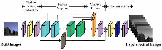
The overall architecture of DRN-DA is shown in Figure 1. DRN-DA falls into four stages, including a shallow feature extraction stage, a feature mapping stage, an adaptive fusion stage, and a reconstruction stage. Let us denote and as the input and output of DRN-DA. Here, 3 or 31 is the band number, N is the batch size, H is the height, and W is the width.
Firstly, we use two 3 × 3 convolutional layers with an activation function called a parametric rectified linear unit (PReLU) [48] between them to extract the shallow features from RGB input images
where represents the shallow feature extraction function. Then, the shallow features are fed to the feature mapping stage for higher-level feature extraction. C is the channel number of the feature map. The procedure can be described as follows:
where represents the feature mapping function, which consists of DRBs and DRABs. is composed of a set of feature maps as
Then, in the adaptive fusion stage, the feature maps extracted by multiple DRBs and DRABs are adaptively fused. This procedure is expressed as
where represents the fusion function described in Section 3.3. At the end of the adaptive fusion stage, global residual learning is introduced to keep the network stable. For the identity mapping branch, a 5 × 5 convolutional layer is utilized to further process the shallow features. The global residual learning can be formulated as
In the final stage, the global feature representation is reconstructed via a reconstruction module as follows:
where and are the reconstruction module and the function of the network of DRN-DA, respectively. The reconstruction module is composed of an adaptive multi-scale block (AMB) and a 3 × 3 convolutional layer. The AMB block has three branches with multiple scale convolutions, and corresponding weights can be automatically learned to make full use of more important representations. Finally, the convolutional layer is used to compress the dimension to , which is the same as the dimension of the ground-truth HSIs.
3.2. Densely Residual Attention Block
As shown in Figure 1, the backbone of the proposed network DRN-DA is stacked with multiple densely residual blocks (DRB) and densely residual attention blocks (DRAB). As the only difference between DRB and DRAB lies in that DRB does not incorporate attention mechanisms, while DRAB has them, here, only DRAB is described in detail. As shown in Figure 1, DRAB consists of a lightweight dense connection and local residual learning. The lightweight dense connection is inspired by DenseNet [34] to alleviate the vanishing-gradient problem and strengthen feature propagation. However, the feature maps are used as inputs into all subsequent layers in the original DenseNet, which results in the DenseNet becoming wider and wider with increasing depth. Therefore, here, a simplified densely connected network is developed to reduce the computation cost. The output of each multi-scale residual attention block (MRAB) is only used as the input into the following second MRAB. After the feature maps of two consecutive layers are concatenated, a 3 × 3 convolutional layer is added to reduce the dimension, which further lowers the width of the dense connection. The procedure of DRAB can be formulated as
where , , , and denote the input of the first, second, and third MRAB, and the feature map which is output from the third MRAB and processed via a convolutional layer, respectively; is the function of MRAB.
As shown in Figure 1, MRAB is composed of three subcomponents, namely multi-scale residual block (MRB), channel attention (CA), and dual downsampling spatial channel (DDSA). The features are processed by three branches: the first branch is stacked with three MRBs; the second branch consisting of CA is parallel to the second MRB; and the third branch consisting of DDSA is parallel to the second MRB as well. Both CA and DDSA work on the second MRB, and the feature maps are fused with concatenation and compression in the channel dimension. The procedure of MRAB is described by the following equations:
where , , , and denote the input of MRAB and the outputs of the first, second, and third MRB, respectively; , , and represent the functions of MRB, CA and DDSA; ⊗ and ⊕ denote the element-wise multiplication and addition, respectively.
Next, we give more details on the multi-scale residual block (MRB), channel attention (CA), and dual downsampling spatial channel (DDSA).
3.2.1. Multi-Scale Residual Block
Since it has been proven that wider features before the activation layer of the residual block can exploit the multi-level features better [49,50], a multi-scale residual block (MRB) is used in the basic building block MRAB. Different from the MRB in [50], a modified MRB is adopted. Inspired by Inception-V2 [51], the 5 × 5 convolutional layer and the 7 × 7 convolutional layer in the multi-scale convolution block from [50] are replaced by two 3 × 3 convolutional layers and three 3 × 3 convolutional layers, respectively. This strategy is adopted to reduce parameters as well as the computational time, but can make the stacked convolutions reach the same receptive fields as the convolutions in [43]. Additionally, the activation function ReLU is replaced by PReLU to introduce more nonlinearity and accelerate convergence. The MRB in this work consists of several parts: a multi-scale convolution block, a PReLU activation function, a feature fusion bottleneck layer, a 3 × 3 convolution layer, and a local residual learning block (see Figure 2).
Multi-Scale Convolution Block: The computations of the three paths in multi-scale convolution block are formulated as
where , , , and are the input of the multi-scale convolution block and the outputs of the first, second, and third paths; , , , , , and are the 3 × 3 convolutional layer in the first path, the first and second 3 × 3 convolutional layers in the second path, and the first, second, third 3 × 3 convolutional layers in the third path.
Feature Fusion: The feature maps output from three paths are concatenated and activated. As a result, 3 × C feature maps are generated. Then, a 1 × 1 convolutional layer is used to fuse the multi-scale features and compress the number of channels. Finally, a 3 × 3 convolutional layer is employed to extract spatial-wise features. This procedure of feature fusion can be formulated as
Local Residual Learning: considering that there are multiple convolutional layers in the above architecture, local residual learning is used to enhance the feature map. The final output feature map of MRB is given by
3.2.2. Channel Attention
In previous tasks, channel-wise attention has been proven to be efficient to select significant features [29,39,40,42,43]. The channel attention in the MRAB architecture is the same as the SE layer [39] shown in Figure 3. First, the input feature is compressed through a global average pooling and made into a global statistics vector :
Next, two fully-connected (FC) layers are used to obtain a bottleneck. The first FC layer is a channel-reduction layer with reduction ratio r, and the second FC layer restores the number of channels. Between the two FC layers, a PRELU is used to increase the nonlinearity.
Finally, a sigmoid function is applied as a gating mechanism to acquire the channel statistics.
3.2.3. Dual Downsampling Spatial Attention
The non-local self-attention mechanism proposed by Wang [35] can capture the long-range dependencies at all positions throughout the entire image. It has been used in various computer vision applications such as video classification and image recognition, and yields great improvement. However, the standard non-local network consumes a large amount of computational memory since each position’s signal is calculated on the whole image, and the computational cost is prohibitive when the image has a large size. Though region-level non-local modules [42] and patch-level non-local modules [29] reduce computational time to some extent, these methods are not efficient enough yet. To address this problem, modified non-local attention is developed in this work to model spatial correlation. In this attention block, a dual downsampling strategy is used to reduce the channel dimension and the size of the input image as illustrated in Figure 4. Let be the input feature map; then, three convolutions are used to convert into three different feature maps, , , and . Concretely, the three convolutions are in the size , and the latter two convolutions have a stride with t to downsample the image in size. This process can be expressed as
Next, the three feature maps are flattened to , , and . Then, a spatial attention map is calculated through multiplying the transposed first feature map by the second feature map and normalized by a Softmax activation function as
where denotes the Softmax function, and is the spatial attention matrix. Subsequently, the feature map is multiplied by the transposed to acquire the weighted feature map , which is formulated as
At last, is reshaped to and then recovered to the same channel dimension as the input feature map by a 1 × 1 convolution. Therefore, the final output is obtained by
3.3. Adaptive Fusion Block
A traditional fusion structure integrates the hierarchical features from early layers to make full use of features from different levels [28,52]. However, most global fusion blocks treat different layers equally. This causes the network to omit more important information, and the quality of reconstructed image is reduced. Therefore, an efficient structure is developed to make the fusion block more effective. Taking the inter-layer relationships into account, in this work, an adaptive fusion block (AFB) is used to fuse the outputs of all DRBs and DRABs (see Figure 1). Each output has an independent weight that is adaptively and automatically adjusted in [0, 1] according to the training loss. The features from different layers are weighted, concatenated, and fused by a convolution. Mathematically, the procedure can be formulated as
where , , , and are trainable weights representing weights of the first, th DRB, the first and th DRAB, respectively; reduces the channel number.
3.4. Adaptive Multi-Scale Block
For a deep learning network, a larger receptive field usually brings the network better representative capability. In this work, at the tail of the proposed network DRN-DA, an AMB with larger receptive fields than the previous multi-scale convolution block in Figure 2 is added to further improve the performance of the network as shown in Figure 1. The AMB is comprised of three kinds of scale convolutions (see Figure 5) with kernel sizes of 3 × 3, 5 × 5, and 7 × 7. After each convolution, the PReLU function is added to increase nonlinearity, and the other convolution with the same size is used to make the receptive field larger. The weight of each scale branch is automatically learned according to the training loss, which results in a trade-off between the reconstruction quality and parameters. The computational process of AMB can be formulated as
where and represent the input and the output of AMB, respectively; and , , and are the weights of the three branches.
4. Experiments
4.1. Settings
4.1.1. Data Sets
In this section, we perform several experiments to verify the effectiveness of the proposed network on four data sets from the NTIRE 2018 and NTIRE 2020 Spectral Reconstruction Challenges [38,40]. In each challenge, there are two data sets: the “Clean” track and the “Real World” track. The “Clean” track contains noise-free and uncompressed 8-bit RGB images obtained from a CIE 1964 color matching function, and the “Real World” track involves JPEG-compressed 8-bit RGB images created by applying an unknown camera response function to ground truth HSIs. Each track in the NTIRE 2018 challenge has 256 natural images for training and 5 + 10 additional images for validation and testing with a size of 1392 × 1300. The reflectance of HSIs in the NTIRE 2018 challenge is in the range of [0, 4095]. Each track in the NTIRE 2020 challenge has 450 images for training and 10 + 20 additional images for validation and testing with a size of 512 × 482. The reflectance of HSIs in the NTIRE 2020 challenge has been normalized to be in [0, 1]. All the HSIs have 31 bands from 400 nm to 700 nm, with a 10 nm step. Since the official testing HSIs in both challenges are confidential, in this work, the official validation HSIs are used for testing, which is the same as the work [30].
4.1.2. Experimental Configuration
In the proposed DRN-DA, we adopted 2 DRBs and 2 DRABs, namely, = = 2. In the intermediate layers, the number of channel dimension C was 64. The channel reduction ratio r of the CA module was 16, and the channel reduction ratio s and the size reduction ratio t of DDSA module were set to be 8 and 4, respectively.
In the training stage, all the training images were resized to be 64 × 64. The model was trained using a batch size of 32 with the Adam optimizer [53] by setting , , and . The learning rate was initialized as , and the polynomial function was set as the decay policy with power . The training process was terminated at the 100th epoch. The model was trained using a PyTorch framework and a NVIDIA RTX 3090 GPU.
4.1.3. Quantitative Metrics
As in the NTIRE 2018 and NTIRE 2020 challenges [38,40], mean relative absolute error (MRAE) is chosen as the quantitative metric of the proposed method. MRAE is defined as
where and denote the ground-truth and reconstructed spectral vectors of the ith pixel, respectively; N is the total number of pixels.
MRAE represents the spatial distance between the ground-truth and reconstructed spectral curves. In general, a smaller MRAE indicates better performance. Moreover, the peak signal-to-noise ratio (PSNR), structural similarity index (SSIM) [54], and spectral angle mapper index (SAM) [55] are used as complementary measures. PSNR and SSIM measure the similarity between the ground truth and the reconstructed spectra. The higher the measures, the better the quality. SAM denotes the angle between the two spectral vectors. The lower the measure, the better the quality.
4.2. Comparisons with State-of-the-Art Methods
As comparisons, several state-of-the-art methods were selected to be compared with the proposed DRN-DA. These methods included Arad [22], HSCNN-R [25], HSCNN-D [25], PDFM [28,40], AWAN [29], and HDRAN [30]. Arad is a method based on sparse coding, and except for HDRAN, the other methods are the top two methods in the two challenges. In addition, to further improve the performance of DRN-DA and make the results more convincing, an ensemble strategy was introduced; the ensemble DRN-DA is denoted as DRN-DA+. Specifically, DRN-DA was trained three times without adjusting any parameters, and the testing results were averaged into the final results, which can avoid the influence of random factors on the results. For a fair comparison, other CNN-based methods use ensemble strategies as well. As the ensemble strategies in the original papers [25,29], HSCNN-R, HSCNN-D, and AWAN with different depths and widths were trained and denoted as HSCNN-R+, HSCNN-D+, and AWAN+. Similar to DRN-DA+, an ensemble strategy was applied to PDFN and HDRAN, and the corresponding models were denoted as PDFN+ and HDRAN+.
4.2.1. Quantitative Evaluation
The results of the hyperspectral reconstruction are summarized in Table 1 and Table 2. For the “Real World” tracks, a self-ensemble strategy used in [29] was adopted, which means that the RGB testing images were flipped up/down and fed to the network. Then, the mirror output and the original output were averaged into the final results. It is noted that the Arad method is only suitable for the “Clean” tracks since the camera response function generating the “Real World” tracks is unknown. Except for HSCNN-R, HSCNN-D on the NTIRE 2018 data sets and AWAN on the NTIRE 2020 “Clean” track, the other networks learned from scratch.
In Table 1 and Table 2, the best and second-best results are bold and underlined, respectively. As can be seen, the proposed DRN-DA performs better than previous methods. Specifically, compared with the second-best method, DRN-DA brings a decrease in MRAE of 6.19% and 1.43% on the NTIRE 2018 “Clean” track and “Real World” track; it brings a decrease in MRAE of 6.85% and 5.30% on the NTIRE 2020 “Clean” track and “Real World” track. In addition, for other measures, DRN-DA also performs better than or equally well as the second-best method. Overall, the CNN-based methods perform much better than the Arad method.
In Table 3 and Table 4, the best and second-best results are bold and underlined, respectively. It can be seen that the proposed DRN-DA+ also outperforms other methods on the four data sets in terms of MRAE, PSNR, and SAM, though it performs equally with HDRAN+ on the NTIRE 2018 “Real World” track in terms of SSIM. Specifically, compared with the second-best method, it produces a reduction in MRAE of 4.59% and 1.84% on the NTIRE 2018 “Clean” track and “Real World” track and a reduction in MRAE of 5.13% and 4.06% on the NTIRE 2020 “Clean” track and “Real World” track.
4.2.2. Visual Evaluation
In order to compare the reconstruction quality of different methods visually, the error maps of four images on five sampled bands (450 nm, 500 nm, 550 nm, 600 nm, and 650 nm) are shown in Figure 6, Figure 7, Figure 8 and Figure 9. The first and last rows show the ground-truth HSIs and the error maps reconstructed by the proposed DRN-DA, and the middle rows show the error maps reconstructed by other benchmark methods. These error maps are the heat maps of MRAE between the ground truth and the reconstructed spectra. As seen from Figure 6, Figure 7, Figure 8 and Figure 9, for the example images from the NTIRE 2018 “Clean” track, and the NTIRE 2020 “Clean” track and “Real World” track, the superiority of the proposed DRN-DA is more significant at the long wavelength 650 nm; however, for the example image from the NTIRE 2018 “Real World” track, the differences between the proposed DRN-DA and other benchmark methods are larger at the long wavelength 600 nm. On the whole, the proposed method generates smaller spectral errors.
Moreover, two samples from each example image are selected (see Figure 10), and the corresponding spectra recovered by different methods are plotted in Figure 11, Figure 12, Figure 13 and Figure 14, where the black and red curves denote the ground-truth and recovered spectra by the proposed method, and the light blue, green, blue, magenta, cyan, and orange curves represent the recovered spectra from Arad, HSCNN-R, HSCNN-D, PDFN, AWAN, and HDRAN, respectively. It can be observed that the recovered spectra from the proposed DRN-DA are closer to the ground-truth spectra.
4.3. Ablation Study for Different Modules
In this section, an ablation study is carried out on NTIRE 2020 data sets to verify the effects of different ingredients, including CA, DDSA, AMB, and AFB in the proposed network. The results in MRAE are reported in Table 5. is a baseline network, which only contains ordinary convolutions. Based on , CA, DDSA, AMB, and AFB are added in succession to the baseline network to obtain , , , and . The gradual reduction of MRAEs on the two data sets demonstrates that these blocks do work for spectral reconstruction.
4.4. Effectiveness of Multi-Scale Convolution Scheme
To validate the effectiveness of the multi-scale convolution scheme, we experimentally analyzed the effects of multi-scale convolutions based on the NTIRE 2020 data sets. As shown in Table 6, the performance increases with the use of multi-scale convolutions. For the NTIRE 2020 “Clean” track and “Real World” track, the network with multi-scale convolutions gains over the network with 3 × 3 convolutions with 3.86% and 4.14% in terms of MRAE, respectively.
5. Conclusions
In this paper, we propose a deep neural network (DRN-DA) for hyperspectral recovery from a single RGB image. The basic block of DRN-DA adopts a simplified densely connected structure, which can reuse features and avoid the basic block from becoming too wide. Different from the original nonlocal module, a dual downsampling strategy is applied to learn the long-range contextual features with much less computation and memory consumption. The dual downsampling spatial attention module, together with a channel attention module, obtains spatial-wise and channel-wise features in a parallel manner to enhance the discriminative ability of the network. Moreover, the adaptive fusion strategy is utilized to fuse multiple-layer features to explore the correlated information from inter-layers via dynamically computing the weight of each layer. Extensive experiments over four data sets demonstrate that the proposed method provides better performance compared with several state-of-the-art methods. However, the efficiency of the network is not taken into account. In the future, we will work on a lightweight hyperspectral reconstruction network to save runtime. Moreover, we hope that this work can be applied to real-world applications.
Author Contributions
L.W. conceived the study; L.W. trained the model, analyzed the data, and wrote the paper; A.S. and J.Y.H. reviewed and improved the manuscript. All authors have read and agreed to the published version of the manuscript.
Funding
This research was funded by NTNU-CSC Joint Scholarship.
Data Availability Statement
Codes are available at https://drive.google.com/drive/folders/1lH81VjEaxT0Cldg6sZfMzS2qWmDIiCjG?usp=sharing (accessed on 9 June 2022).
Conflicts of Interest
The authors declare no conflict of interest.
References
- Pelagotti, A.; Del Mastio, A.; De Rosa, A.; Piva, A. Multispectral imaging of paintings. IEEE Signal Process. Mag. 2008, 25, 27–36. [Google Scholar] [CrossRef]
- Chane, C.S.; Mansouri, A.; Marzani, F.S.; Boochs, F. Integration of 3D and multispectral data for cultural heritage applications: Survey and perspectives. Image Vis. Comput. 2013, 31, 91–102. [Google Scholar] [CrossRef] [Green Version]
- Nishidate, I.; Maeda, T.; Niizeki, K.; Aizu, Y. Estimation of melanin and hemoglobin using spectral reflectance images reconstructed from a digital RGB image by the Wiener estimation method. Sensors 2013, 13, 7902–7915. [Google Scholar] [CrossRef] [PubMed] [Green Version]
- Yuen, P.W.; Richardson, M. An introduction to hyperspectral imaging and its application for security, surveillance and target acquisition. Imaging Sci. J. 2010, 58, 241–253. [Google Scholar] [CrossRef]
- Chao, K.; Yang, C.C.; Chen, Y.; Kim, M.; Chan, D. Hyperspectral-multispectral line-scan imaging system for automated poultry carcass inspection applications for food safety. Poult. Sci. 2007, 86, 2450–2460. [Google Scholar] [CrossRef]
- Valero, E.M.; Hu, Y.; Hernández-Andrés, J.; Eckhard, T.; Nieves, J.L.; Romero, J.; Schnitzlein, M.; Nowack, D. Comparative performance analysis of spectral estimation algorithms and computational optimization of a multispectral imaging system for print inspection. Color Res. Appl. 2014, 39, 16–27. [Google Scholar] [CrossRef]
- Pan, Z.; Healey, G.; Prasad, M.; Tromberg, B. Face recognition in hyperspectral images. IEEE Trans. Pattern Anal. Mach. Intell. 2003, 25, 1552–1560. [Google Scholar]
- Van Nguyen, H.; Banerjee, A.; Chellappa, R. Tracking via object reflectance using a hyperspectral video camera. In Proceedings of the 2010 IEEE Computer Society Conference on Computer Vision and Pattern Recognition-Workshops, San Francisco, CA, USA, 13–18 June 2010; IEEE: Piscataway, NJ, USA, 2010; pp. 44–51. [Google Scholar]
- Li, J.; Du, Q.; Li, Y.; Li, W. Hyperspectral image classification with imbalanced data based on orthogonal complement subspace projection. IEEE Trans. Geosci. Remote Sens. 2018, 56, 3838–3851. [Google Scholar] [CrossRef]
- Wu, F.; Duan, J.; Chen, S.; Ye, Y.; Ai, P.; Yang, Z. Multi-target recognition of bananas and automatic positioning for the inflorescence axis cutting point. Front. Plant Sci. 2021, 12, 705021. [Google Scholar] [CrossRef]
- Tang, Y.; Zhu, M.; Chen, Z.; Wu, C.; Chen, B.; Li, C.; Li, L. Seismic performance evaluation of recycled aggregate concrete-filled steel tubular columns with field strain detected via a novel mark-free vision method. Structures 2022, 37, 426–441. [Google Scholar] [CrossRef]
- Green, R.O.; Eastwood, M.L.; Sarture, C.M.; Chrien, T.G.; Aronsson, M.; Chippendale, B.J.; Faust, J.A.; Pavri, B.E.; Chovit, C.J.; Solis, M.; et al. Imaging spectroscopy and the airborne visible/infrared imaging spectrometer (AVIRIS). Remote Sens. Environ. 1998, 65, 227–248. [Google Scholar] [CrossRef]
- Hearn, D.; Digenis, C.; Lencioni, D.; Mendenhall, J.; Evans, J.; Welsh, R. EO-1 advanced land imager overview and spatial performance. In Proceedings of the IGARSS 2001, Scanning the Present and Resolving the Future, IEEE 2001 International Geoscience and Remote Sensing Symposium (Cat. No. 01CH37217), Sydney, Australia, 9–13 July 2001; IEEE: Piscataway, NJ, USA, 2001; Volume 2, pp. 897–900. [Google Scholar]
- Hagen, N.A.; Gao, L.S.; Tkaczyk, T.S.; Kester, R.T. Snapshot advantage: A review of the light collection improvement for parallel high-dimensional measurement systems. Opt. Eng. 2012, 51, 111702. [Google Scholar] [CrossRef] [PubMed]
- Li, Q.; He, X.; Wang, Y.; Liu, H.; Xu, D.; Guo, F. Review of spectral imaging technology in biomedical engineering: Achievements and challenges. J. Biomed. Opt. 2013, 18, 100901. [Google Scholar] [CrossRef] [PubMed] [Green Version]
- Shen, H.L.; Cai, P.Q.; Shao, S.J.; Xin, J.H. Reflectance reconstruction for multispectral imaging by adaptive Wiener estimation. Opt. Express 2007, 15, 15545–15554. [Google Scholar] [CrossRef] [PubMed] [Green Version]
- Zhang, W.F.; Tang, G.; Dai, D.Q.; Nehorai, A. Estimation of reflectance from camera responses by the regularized local linear model. Opt. Lett. 2011, 36, 3933–3935. [Google Scholar] [CrossRef]
- Wang, L.; Wan, X.; Xiao, G.; Liang, J. Sequential adaptive estimation for spectral reflectance based on camera responses. Opt. Express 2020, 28, 25830–25842. [Google Scholar] [CrossRef]
- Nguyen, R.M.; Prasad, D.K.; Brown, M.S. Training-based spectral reconstruction from a single RGB image. In Proceedings of the European Conference on Computer Vision, Zurich, Switzerland, 6–12 September 2014; Springer: Berlin/Heidelberg, Germany, 2014; pp. 186–201. [Google Scholar]
- Aeschbacher, J.; Wu, J.; Timofte, R. In defense of shallow learned spectral reconstruction from rgb images. In Proceedings of the IEEE International Conference on Computer Vision Workshops, Venice, Italy, 22–29 October 2017; pp. 471–479. [Google Scholar]
- Robles-Kelly, A. Single image spectral reconstruction for multimedia applications. In Proceedings of the 23rd ACM international conference on Multimedia, Brisbane, Australia, 26–30 October 2015; pp. 251–260. [Google Scholar]
- Arad, B.; Ben-Shahar, O. Sparse recovery of hyperspectral signal from natural RGB images. In Proceedings of the European Conference on Computer Vision, Amsterdam, The Netherlands, 11–14 October 2016; Springer: Berlin/Heidelberg, Germany, 2016; pp. 19–34. [Google Scholar]
- Jia, Y.; Zheng, Y.; Gu, L.; Subpa-Asa, A.; Lam, A.; Sato, Y.; Sato, I. From RGB to spectrum for natural scenes via manifold-based mapping. In Proceedings of the IEEE International Conference on Computer Vision, Venice, Italy, 22–29 October 2017; pp. 4705–4713. [Google Scholar]
- Xiong, Z.; Shi, Z.; Li, H.; Wang, L.; Liu, D.; Wu, F. Hscnn: Cnn-based hyperspectral image recovery from spectrally undersampled projections. In Proceedings of the IEEE International Conference on Computer Vision Workshops, Venice, Italy, 22–29 October 2017; pp. 518–525. [Google Scholar]
- Shi, Z.; Chen, C.; Xiong, Z.; Liu, D.; Wu, F.H. Advanced cnn-based hyperspectral recovery from rgb images. In Proceedings of the 2018 IEEE/CVF Conference on Computer Vision and Pattern Recognition Workshops (CVPRW), Salt Lake City, UT, USA, 18–22 June 2018; pp. 18–22. [Google Scholar]
- Zhang, J.; Sun, Y.; Chen, J.; Yang, D.; Liang, R. Deep-learning-based hyperspectral recovery from a single RGB image. Opt. Lett. 2020, 45, 5676–5679. [Google Scholar] [CrossRef]
- Zhao, Y.; Po, L.M.; Yan, Q.; Liu, W.; Lin, T. Hierarchical regression network for spectral reconstruction from RGB images. In Proceedings of the IEEE/CVF Conference on Computer Vision and Pattern Recognition Workshops, Seattle, WA, USA, 14–19 June 2020; pp. 422–423. [Google Scholar]
- Zhang, L.; Lang, Z.; Wang, P.; Wei, W.; Liao, S.; Shao, L.; Zhang, Y. Pixel-aware deep function-mixture network for spectral super-resolution. In Proceedings of the AAAI Conference on Artificial Intelligence, New York, NY, USA, 7–12 February 2020; Volume 34, pp. 12821–12828. [Google Scholar]
- Li, J.; Wu, C.; Song, R.; Li, Y.; Liu, F. Adaptive weighted attention network with camera spectral sensitivity prior for spectral reconstruction from RGB images. In Proceedings of the IEEE/CVF Conference on Computer Vision and Pattern Recognition Workshops, Seattle, WA, USA, 14–19 June 2020; pp. 462–463. [Google Scholar]
- Li, J.; Wu, C.; Song, R.; Xie, W.; Ge, C.; Li, B.; Li, Y. Hybrid 2-D–3-D Deep Residual Attentional Network With Structure Tensor Constraints for Spectral Super-Resolution of RGB Images. IEEE Trans. Geosci. Remote Sens. 2020, 59, 2321–2335. [Google Scholar] [CrossRef]
- Zhang, J.; Zhao, D.; Chen, J.; Sun, Y.; Yang, D.; Liang, R. Unsupervised learning for hyperspectral recovery based on a single RGB image. Opt. Lett. 2021, 46, 3977–3980. [Google Scholar] [CrossRef]
- Lore, K.G.; Reddy, K.K.; Giering, M.; Bernal, E.A. Generative adversarial networks for spectral super-resolution and bidirectional rgb-to-multispectral mapping. In Proceedings of the 2019 IEEE/CVF Conference on Computer Vision and Pattern Recognition Workshops (CVPRW), Long Beach, CA, USA, 16–17 June 2019; IEEE: Piscataway, NJ, USA, 2019; pp. 926–933. [Google Scholar]
- Liu, P.; Zhao, H. Adversarial Networks for Scale Feature-Attention Spectral Image Reconstruction from a Single RGB. Sensors 2020, 20, 2426. [Google Scholar] [CrossRef]
- Huang, G.; Liu, Z.; Van Der Maaten, L.; Weinberger, K.Q. Densely connected convolutional networks. In Proceedings of the IEEE conference on computer vision and pattern recognition, Honolulu, HI, USA, 21–26 July 2017; pp. 4700–4708. [Google Scholar]
- Wang, X.; Girshick, R.; Gupta, A.; He, K. Non-local neural networks. In Proceedings of the IEEE Conference on Computer Vision and Pattern Recognition, Salt Lake City, UT, USA, 18–23 June 2018; pp. 7794–7803. [Google Scholar]
- He, K.; Zhang, X.; Ren, S.; Sun, J. Deep residual learning for image recognition. In Proceedings of the IEEE Conference on Computer Vision and Pattern Recognition, Las Vegas, NV, USA, 27–30 June 2016; pp. 770–778. [Google Scholar]
- Kim, J.; Lee, J.K.; Lee, K.M. Accurate image super-resolution using very deep convolutional networks. In Proceedings of the IEEE Conference on Computer Vision and Pattern Recognition, Las Vegas, NV, USA, 27–30 June 2016; pp. 1646–1654. [Google Scholar]
- Arad, B.; Ben-Shahar, O.; Timofte, R. Ntire 2018 challenge on spectral reconstruction from rgb images. In Proceedings of the IEEE Conference on Computer Vision and Pattern Recognition Workshops, Salt Lake City, UT, USA, 18–22 June 2018; pp. 929–938. [Google Scholar]
- Hu, J.; Shen, L.; Sun, G. Squeeze-and-excitation networks. In Proceedings of the IEEE Conference on Computer Vision and Pattern Recognition, Salt Lake City, UT, USA, 18–23 June 2018; pp. 7132–7141. [Google Scholar]
- Arad, B.; Timofte, R.; Ben-Shahar, O.; Lin, Y.T.; Finlayson, G.D. Ntire 2020 challenge on spectral reconstruction from an rgb image. In Proceedings of the IEEE/CVF Conference on Computer Vision and Pattern Recognition Workshops, Seattle, WA, USA, 14–19 June 2020; pp. 446–447. [Google Scholar]
- Mnih, V.; Heess, N.; Graves, A.; Kavukcuoglu, A. Recurrent models of visual attention. In Proceedings of the Advances in Neural Information Processing Systems, Montreal, QC, Canada, 8–13 December 2014; pp. 2204–2212. [Google Scholar]
- Dai, T.; Cai, J.; Zhang, Y.; Xia, S.T.; Zhang, L. Second-order attention network for single image super-resolution. In Proceedings of the IEEE/CVF Conference on Computer Vision and Pattern Recognition, Long Beach, CA, USA, 15–20 June 2019; pp. 11065–11074. [Google Scholar]
- Anwar, S.; Barnes, N. Densely residual laplacian super-resolution. IEEE Trans. Pattern Anal. Mach. Intell. 2020, 44, 1192–1204. [Google Scholar] [CrossRef] [PubMed]
- Wang, C.; Li, Z.; Shi, J. Lightweight image super-resolution with adaptive weighted learning network. arXiv 2019, arXiv:1904.02358. [Google Scholar]
- Chen, L.; Yang, X.; Jeon, G.; Anisetti, M.; Liu, K. A trusted medical image super-resolution method based on feedback adaptive weighted dense network. Artif. Intell. Med. 2020, 106, 101857. [Google Scholar] [CrossRef] [PubMed]
- Liu, R.; Mi, L.; Chen, Z. AFNet: Adaptive fusion network for remote sensing image semantic segmentation. IEEE Trans. Geosci. Remote Sens. 2020, 59, 7871–7886. [Google Scholar] [CrossRef]
- Gao, H.; Chen, Z.; Xu, F. Adaptive spectral-spatial feature fusion network for hyperspectral image classification using limited training samples. Int. J. Appl. Earth Obs. Geoinf. 2022, 107, 102687. [Google Scholar] [CrossRef]
- He, K.; Zhang, X.; Ren, S.; Sun, J. Delving deep into rectifiers: Surpassing human-level performance on imagenet classification. In Proceedings of the IEEE International Conference on Computer Vision, Santiago, Chile, 7–13 December 2015; pp. 1026–1034. [Google Scholar]
- Yu, J.; Fan, Y.; Yang, J.; Xu, N.; Wang, Z.; Wang, X.; Huang, T. Wide activation for efficient and accurate image super-resolution. arXiv 2018, arXiv:1808.08718. [Google Scholar]
- Zhang, S.; Yuan, Q.; Li, J.; Sun, J.; Zhang, X. Scene-adaptive remote sensing image super-resolution using a multiscale attention network. IEEE Trans. Geosci. Remote Sens. 2020, 58, 4764–4779. [Google Scholar] [CrossRef]
- Ioffe, S.; Szegedy, C. Batch normalization: Accelerating deep network training by reducing internal covariate shift. In Proceedings of the International Conference on Machine Learning (PMLR), Lille, France, 6–11 July 2015; pp. 448–456. [Google Scholar]
- Jiang, K.; Wang, Z.; Yi, P.; Jiang, J. Hierarchical dense recursive network for image super-resolution. Pattern Recognit. 2020, 107, 107475. [Google Scholar] [CrossRef]
- Kingma, D.P.; Ba, J. Adam: A method for stochastic optimization. arXiv 2014, arXiv:1412.6980. [Google Scholar]
- Wang, Z.; Bovik, A.C.; Sheikh, H.R.; Simoncelli, E.P. Image quality assessment: From error visibility to structural similarity. IEEE Trans. Image Process. 2004, 13, 600–612. [Google Scholar] [CrossRef] [Green Version]
- Yuhas, R.H.; Boardman, J.W.; Goetz, A.F. Determination of semi-arid landscape endmembers and seasonal trends using convex geometry spectral unmixing techniques. In Proceedings of the JPL, Summaries of the 4th Annual JPL Airborne Geoscience Workshop, Washington, DC, USA, 25–29 October 1993; Volume 1. [Google Scholar]
Figure 1.
Network architecture of DRN-DA.

Figure 2.
Multi-scale residual block (MRB).

Figure 3.
Channel attention (CA) module.

Figure 4.
Dual downsampling spatial attention (DDSA) module.

Figure 5.
Adaptive multi-scale block (AMB).

Figure 6.
Visual hyperspectral reconstruction results and visual comparisons of five selected bands for hyperspectral reconstruction error maps from one NTIRE 2018 “Clean” RGB image. The significant differences are shown in the red frames. Please zoom in for better view.
Figure 6.
Visual hyperspectral reconstruction results and visual comparisons of five selected bands for hyperspectral reconstruction error maps from one NTIRE 2018 “Clean” RGB image. The significant differences are shown in the red frames. Please zoom in for better view.

Figure 7.
Visual hyperspectral reconstruction results and visual comparisons of five selected bands for hyperspectral reconstruction error maps from one NTIRE 2018 “Real World” RGB image. The significant differences are shown in the red frames. Please zoom in for better view.
Figure 7.
Visual hyperspectral reconstruction results and visual comparisons of five selected bands for hyperspectral reconstruction error maps from one NTIRE 2018 “Real World” RGB image. The significant differences are shown in the red frames. Please zoom in for better view.

Figure 8.
Visual hyperspectral reconstruction results and visual comparisons of five selected bands for hyperspectral reconstruction error maps from one NTIRE 2020 “Clean” RGB image. The significant differences are shown in the red frames. Please zoom in for better view.
Figure 8.
Visual hyperspectral reconstruction results and visual comparisons of five selected bands for hyperspectral reconstruction error maps from one NTIRE 2020 “Clean” RGB image. The significant differences are shown in the red frames. Please zoom in for better view.

Figure 9.
Visual hyperspectral reconstruction results and visual comparisons of five selected bands for hyperspectral reconstruction error maps from one NTIRE 2020 “Real World” RGB image. The significant differences are shown in the red frames. Please zoom in for better view.
Figure 9.
Visual hyperspectral reconstruction results and visual comparisons of five selected bands for hyperspectral reconstruction error maps from one NTIRE 2020 “Real World” RGB image. The significant differences are shown in the red frames. Please zoom in for better view.

Figure 10.
Two selected samples in each example image. (a) NTIRE 2018 “Clean” track. (b) NTIRE 2018 “Real Word” track. (c) NTIRE 2020 “Clean” track. (d) NTIRE 2020 “Real Word” track.
Figure 10.
Two selected samples in each example image. (a) NTIRE 2018 “Clean” track. (b) NTIRE 2018 “Real Word” track. (c) NTIRE 2020 “Clean” track. (d) NTIRE 2020 “Real Word” track.

Figure 11.
Spectral reflectance of selected samples from NTIRE 2018 “Clean” track. (a) Sample 1. (b) Sample 2.
Figure 11.
Spectral reflectance of selected samples from NTIRE 2018 “Clean” track. (a) Sample 1. (b) Sample 2.

Figure 12.
Spectral reflectance of selected samples from the NTIRE 2018 “Real World” track: (a) Sample 1. (b) Sample 2.
Figure 12.
Spectral reflectance of selected samples from the NTIRE 2018 “Real World” track: (a) Sample 1. (b) Sample 2.

Figure 13.
Spectral reflectance of selected samples from the NTIRE 2020 “Clean” track. (a) Sample 1. (b) Sample 2.
Figure 13.
Spectral reflectance of selected samples from the NTIRE 2020 “Clean” track. (a) Sample 1. (b) Sample 2.

Figure 14.
Spectral reflectance of selected samples from the NTIRE 2020 “Real World” track. (a) Sample 1. (b) Sample 2.
Figure 14.
Spectral reflectance of selected samples from the NTIRE 2020 “Real World” track. (a) Sample 1. (b) Sample 2.


Table 1.
Comparison between the proposed method and other state-of-the-art methods without the ensemble strategy based on the NTIRE 2018 data sets.
Table 1.
Comparison between the proposed method and other state-of-the-art methods without the ensemble strategy based on the NTIRE 2018 data sets.
| Method | NTIRE 2018 | |||||||
|---|---|---|---|---|---|---|---|---|
| Clean | Real World | |||||||
| MRAE | PSNR | SAM | SSIM | MRAE | PSNR | SAM | SSIM | |
| Arad | 0.0746 | 34.4848 | 4.8086 | 0.9507 | - | - | - | - |
| HSCNN-R | 0.0140 | 49.9568 | 1.0432 | 0.9988 | 0.0303 | 45.2228 | 1.6176 | 0.9952 |
| HSCNN-D | 0.0135 | 50.4873 | 0.9929 | 0.9988 | 0.0293 | 45.3876 | 1.5944 | 0.9953 |
| PDFN | 0.0124 | 51.5143 | 0.9013 | 0.9990 | 0.0288 | 45.7187 | 1.5197 | 0.9956 |
| AWAN | 0.0115 | 52.2588 | 0.8022 | 0.9993 | 0.0287 | 45.7325 | 1.5035 | 0.9956 |
| HDRAN | 0.0113 | 52.1924 | 0.8038 | 0.9992 | 0.0279 | 45.8122 | 1.4578 | 0.9957 |
| DRN-DA | 0.0106 | 52.9249 | 0.7478 | 0.9994 | 0.0275 | 45.9295 | 1.4501 | 0.9957 |
Table 2.
Comparison between the proposed method and other state-of-the-art methods without the ensemble strategy based on the NTIRE 2020 data sets.
Table 2.
Comparison between the proposed method and other state-of-the-art methods without the ensemble strategy based on the NTIRE 2020 data sets.
| Method | NTIRE 2020 | |||||||
|---|---|---|---|---|---|---|---|---|
| Clean | Real World | |||||||
| MRAE | PSNR | SAM | SSIM | MRAE | PSNR | SAM | SSIM | |
| Arad | 0.0886 | 30.0583 | 6.3112 | 0.9366 | - | - | - | - |
| HSCNN-R | 0.0389 | 38.4837 | 2.6834 | 0.9905 | 0.0687 | 35.8132 | 3.5955 | 0.9777 |
| HSCNN-D | 0.0383 | 39.0426 | 2.6330 | 0.9915 | 0.0702 | 35.8528 | 3.5633 | 0.9760 |
| PDFN | 0.0362 | 40.2493 | 2.4051 | 0.9936 | 0.0674 | 35.9353 | 3.4106 | 0.9781 |
| AWAN | 0.0321 | 40.7767 | 2.2108 | 0.9940 | 0.0666 | 36.2859 | 3.3793 | 0.9793 |
| HDRAN | 0.0338 | 40.3583 | 2.2706 | 0.9941 | 0.0660 | 36.2287 | 3.2887 | 0.9777 |
| DRN-DA | 0.0299 | 41.3852 | 2.0516 | 0.9952 | 0.0625 | 36.8841 | 3.0945 | 0.9814 |
Table 3.
Comparison between the proposed method and other state-of-the-art methods with the ensemble strategy based on the NTIRE 2018 data sets.
Table 3.
Comparison between the proposed method and other state-of-the-art methods with the ensemble strategy based on the NTIRE 2018 data sets.
| Method | NTIRE 2018 | |||||||
|---|---|---|---|---|---|---|---|---|
| Clean | Real World | |||||||
| MRAE | PSNR | SAM | SSIM | MRAE | PSNR | SAM | SSIM | |
| HSCNN-R+ | 0.0135 | 50.4526 | 0.9919 | 0.9989 | 0.0297 | 45.3689 | 1.5889 | 0.9953 |
| HSCNN-D+ | 0.0132 | 50.6399 | 0.9829 | 0.9988 | 0.0287 | 45.5924 | 1.5469 | 0.9955 |
| PDMN+ | 0.0120 | 51.6619 | 0.8742 | 0.9991 | 0.0283 | 45.8206 | 1.5066 | 0.9956 |
| AWAN+ | 0.0112 | 52.4566 | 0.7823 | 0.9993 | 0.0282 | 45.8196 | 1.4788 | 0.9957 |
| HDRAN+ | 0.0109 | 52.4758 | 0.7712 | 0.9993 | 0.0277 | 45.9015 | 1.4481 | 0.9958 |
| DRN-DA+ | 0.0104 | 53.0600 | 0.7358 | 0.9994 | 0.0272 | 45.9864 | 1.4311 | 0.9958 |
Table 4.
Comparison between the proposed method and other state-of-the-art methods with the ensemble strategy based on the NTIRE 2020 data sets.
Table 4.
Comparison between the proposed method and other state-of-the-art methods with the ensemble strategy based on the NTIRE 2020 data sets.
| Method | NTIRE 2020 | |||||||
|---|---|---|---|---|---|---|---|---|
| Clean | Real World | |||||||
| MRAE | PSNR | SAM | SSIM | MRAE | PSNR | SAM | SSIM | |
| HSCNN-R+ | 0.0372 | 39.2337 | 2.5544 | 0.9920 | 0.0673 | 36.0495 | 3.4131 | 0.9785 |
| HSCNN-D+ | 0.0377 | 39.1697 | 2.6012 | 0.9918 | 0.0696 | 36.0132 | 3.5028 | 0.9767 |
| PDMN+ | 0.0331 | 40.4981 | 2.2144 | 0.9985 | 0.0660 | 36.1770 | 3.3103 | 0.9789 |
| AWAN+ | 0.0312 | 40.9987 | 2.1552 | 0.9943 | 0.0646 | 36.2757 | 3.2328 | 0.9795 |
| HDRAN+ | 0.0337 | 40.4786 | 2.2611 | 0.9937 | 0.0640 | 36.4580 | 3.2030 | 0.9793 |
| DRN-DA+ | 0.0296 | 41.4652 | 2.0279 | 0.9954 | 0.0614 | 36.8029 | 3.0351 | 0.9811 |
Table 5.
Effects of different ingredients in the proposed network.
| CA | ✗ | ✔ | ✔ | ✔ | ✔ |
| DDSA | ✗ | ✗ | ✔ | ✔ | ✔ |
| AMB | ✗ | ✗ | ✗ | ✔ | ✔ |
| AFB | ✗ | ✗ | ✗ | ✗ | ✔ |
| Clean | 0.0371 | 0.0348 | 0.0343 | 0.0338 | 0.0299 |
| Real World | 0.0670 | 0.0652 | 0.0649 | 0.0637 | 0.0625 |
Table 6.
Effects of multi-scale convolutions in the proposed network.
| Multi-scale convolutions | ✗ | ✔ |
| Clean | 0.0311 | 0.0299 |
| Real World | 0.0652 | 0.0625 |
Publisher’s Note: MDPI stays neutral with regard to jurisdictional claims in published maps and institutional affiliations. |
© 2022 by the authors. Licensee MDPI, Basel, Switzerland. This article is an open access article distributed under the terms and conditions of the Creative Commons Attribution (CC BY) license (https://creativecommons.org/licenses/by/4.0/).
Share and Cite
MDPI and ACS Style
Wang, L.; Sole, A.; Hardeberg, J.Y. Densely Residual Network with Dual Attention for Hyperspectral Reconstruction from RGB Images. Remote Sens. 2022, 14, 3128. https://0-doi-org.brum.beds.ac.uk/10.3390/rs14133128
AMA Style
Wang L, Sole A, Hardeberg JY. Densely Residual Network with Dual Attention for Hyperspectral Reconstruction from RGB Images. Remote Sensing. 2022; 14(13):3128. https://0-doi-org.brum.beds.ac.uk/10.3390/rs14133128
Chicago/Turabian StyleWang, Lixia, Aditya Sole, and Jon Yngve Hardeberg. 2022. "Densely Residual Network with Dual Attention for Hyperspectral Reconstruction from RGB Images" Remote Sensing 14, no. 13: 3128. https://0-doi-org.brum.beds.ac.uk/10.3390/rs14133128
Note that from the first issue of 2016, this journal uses article numbers instead of page numbers. See further details here.