Article

GNSS-R Soil Moisture Retrieval for Flat Vegetated Surfaces Using a Physics-Based Bistatic Scattering Model and Hybrid Global/Local Optimization

1
Ming Hsieh Department of Electrical and Computer Engineering, University of Southern California, Los Angeles, CA 90089, USA
2
Department of Civil Engineering, Monash University, Clayton, VIC 3800, Australia
*
Author to whom correspondence should be addressed.
Remote Sens. 2022, 14(13), 3129; https://0-doi-org.brum.beds.ac.uk/10.3390/rs14133129
Submission received: 23 May 2022 / Revised: 19 June 2022 / Accepted: 24 June 2022 / Published: 29 June 2022

Abstract

:
This paper presents a soil moisture retrieval scheme from Cyclone Global Navigation Satellite System (CYGNSS) delay-Doppler maps (DDMs) over land. The proposed inversion method consists of a hybrid global and local optimization method and a physics-based bistatic scattering forward model. The forward model was developed for bare-to-densely vegetated terrains, and it predicts the circularly polarized bistatic radar cross section DDM of the land surface. This method was tested on both simulated DDMs and CYGNSS DDMs over the Soil Moisture Active Passive (SMAP) Yanco core validation site in Australia. About 250 CYGNSS DDMs from 2019 and 2020 over the Yanco site were used for validation. The simulated DDMs were for grassland and forest vegetation types. The vegetation type of the Yanco validation site was grassland. The vegetation water content (VWC) was 0.19   kg m 2 and 4.89   kg m 2 for the grassland and forest terrains, respectively. For the case when the surface roughness is known to the algorithm, the unbiased root mean square error (ubRMSE) of soil moisture estimates was less than 0.03   m 3 m 3 while it was approximately 0.06   m 3 m 3 and 0.09   m 3 m 3 for the validation results from 2019 and 2020, respectively. The retrieval algorithm generally had enhanced performance for smaller values of soil moisture. For the case when both the soil moisture and surface roughness are unknown to the algorithm and only a single DDM is used for retrieval, the validation results showed an expected reduced performance, with an an ubRMSE of less than 0.12   m 3 m 3 .

Graphical Abstract

1. Introduction

Soil moisture is a key variable in studying the global ecosystems. Soil moisture measurements on global and local scales provide essential information for analyzing the processes of evapotranspiration and groundwater recharge. Thus, quantifying soil moisture values leads to a better understanding of the water, carbon, and energy cycles [1]. As global concern about the impact of climate change continues to grow, studies on soil moisture variation have become even more important. Soil moisture observations contribute to many areas of human interest, including flood and landslide prediction, weather forecasting, drought analysis, wildfire prevention, crop productivity evaluation, and human health.
Over the past decade, many approaches have been investigated to measure soil moisture on local and global scales using monostatic radars as an active mode of microwave remote sensing [1,2,3,4,5]. Furthermore, passive microwave observations are also widely used to measure soil moisture [1,6]. A radar system has a transmitter (active mode) for observations, whereas a radiometer uses brightness temperature (emission) to make passive measurements. The conventional spaceborne and airborne monostatic radar systems for soil moisture observation include National Aeronautics and Space Administration (NASA) Soil Moisture Active Passive (SMAP) [1] when the radar was operational, NASA/Jet Propulsion Laboratory (JPL) Uninhabited Aerial Vehicle Synthetic Aperture Radar (UAVSAR) [7], the Airborne Microwave Observatory of Subcanopy and Subsurface (AirMOSS) [8], the Polarimetric L-band Imaging SAR (PLIS) [9], and the Environmental Satellite (EnviSat) [10], among others. The passive systems include European Space Agency (ESA) Soil Moisture and Ocean Salinity (SMOS) mission [6], NASA SMAP [1], and Polarimetric L-band Multi-beam Radiometer (PLMR) [11], among others.
Conventional monostatic radars in general offer higher spatial resolution. However, they are expensive, and it would be a total loss should the transmitter fail. For example, the NASA SMAP radar failed in 2015, approximately three months after commissioning. To overcome the barriers of conventional monostatic radar systems, it is possible to use bistatic or multi-static radars, which have the capability of receiving the scattered signals from all directions within the beam-widths of receiving antennas, and creating a data space of higher dimensionality. Using them enables retrieving scattered field measurements via passive receiver systems, which are simpler and less expensive than the monostatic radars and have the potential to provide more accurate soil moisture retrievals with higher spatial and temporal resolution. Studies recently focused on the use of signals of opportunity (SoOp) for addressing the soil moisture observation challenges on local and global scales [12,13].
SoOp includes signals transmitted from global navigation satellite system (GNSS) and communications satellites. Due to the pervasive presence and reliability of L-band Global Positioning System (GPS)/GNSS signals, using SoOp from GPS/GNSS satellites for soil moisture retrieval has been receiving increasing attention in recent years [14,15,16,17]. For instance, NASA Cyclone GNSS (CYGNSS) was originally designed and used for sensing sea level wind speed in tropical cyclones from GNSS signals [18]. Recently, it was used for observations over land [19]. CYGNSS uses a constellation of eight satellites in low Earth orbit (LEO) at 35° orbit inclination. Each CYGNSS satellite is equipped with a four-channel GNSS bistatic radar receiver, which is capable of bistatic radar measurements of GNSS-reflectometry (GNSS-R) from land and ocean surfaces. Unlike conventional monostatic radars, the CYGNSS receivers and the GPS transmitters are not collocated. Instead, the CYGNSS satellites measure GPS signals that have been scattered from land and ocean surfaces in the vicinity of the specular direction (glistening zone) [18]. The CYGNSS level-1a and level-1b data products present the received power and the bistatic radar cross section (BRCS), respectively, in the form of a delay-Doppler map (DDM) [18].
Previous approaches for soil moisture retrieval from CYGNSS observations include empirical- and machine learning (ML)-based methods. An example of the empirical retrieval techniques is the UCAR/CU retrieval algorithm [20]. Chew et al. [20] presented a method for soil moisture retrieval, which uses the CYGNSS data, calibrated to the SMAP soil moisture data. According to [20], this retrieval algorithm has limitations, including potential errors in SMAP retrieved soil moisture data, using a preliminary vegetation model, which only addresses the attenuation due to the vegetation layer, and a low spatial resolution (36 km). Moreover, Senyurek et al. [21] presented an ML-based model for soil moisture retrieval from CYGNSS data over International Soil Moisture Network (ISMN) sites in the Continental United States (CONUS). They compared three different ML-based approaches, namely artificial neural network (ANN), random forests (RF), and support vector machine (SVM) for soil moisture retrieval from CYGNSS data. In [22], the authors extended their retrievals from CONUS to the CYGNSS global coverage. Furthermore, they included retrievals from more densely vegetated terrains, compared to their previous work. Only the RF ML-based approach was used. The ISMN sites were used for the training, and SMAP observations were used for validations. Some of the limitations in [21] were addressed in [22]. Al-Khaldi et al. [23,24] presented a time-series-based method for retrieving soil moisture from CYGNSS data. This method uses Hagfors’ law for computing the incoherent scattering component and retrieves a three-day soil moisture value using multiple observations with different incidence angles. Considering the limitations in the existing retrievals methods based on empirical or data-based approaches, it is worthwhile to use a physics-based microwave bistatic scattering model for soil moisture retrieval from GNSS-R. Physics-based methods are more resistant to site bias and may provide more accurate retrievals for scenarios that were not in the training/fitting data.
In our previous works, we reported on a polarimetric bistatic scattering forward model, which uses the approximate solution of Maxwell’s equations [12,25,26]. In this model called Single-Species Bistatic scattering Model (SSBM) [27], the scattered wave was formulated based on the distorted Born approximation (DBA). In this paper, the SSBM, was used in an inversion algorithm for soil moisture retrieval from CYGNSS DDMs over land. We note that it is also possible to use any other available and validated bistatic forward scattering model for this purpose, and that the choice of SSBM is made due to the fact that we developed and validated this model and have ready access to it. The SSBM has three main categories of contributions: (1) direct bistatic scattering from the rough ground surface with the assumption of flat topography, (2) direct bistatic scattering from the vegetation layer, and (3) double-bounce bistatic scattering from the vegetation layer and ground. In order to simulate the CYGNSS observations (DDMs), the SSBM was used to predict the circularly polarized BRCS of the region of interest observed by CYGNSS satellites [25]. The circularly polarized BRCS values computed by the forward model were then used to construct the desired DDM. The inversion technique proposed in this paper is based on the hybrid global and local optimization method of [28]. The hybrid global and local optimization scheme used in the inversion algorithm takes advantage of the speed of a local optimization method while ensuring convergence to the global minimum of the inverse problem [28]. Compared to the conventional simulated annealing methods, this optimization technique was shown to be faster and more accurate [28]. The proposed inversion method was developed and validated in simulation, as well as with data over the SMAP Yanco site located in Australia. The retrieved soil moisture values were validated with the Yanco in situ soil moisture sensor measurements.
This paper is structured as follows: A summary of the SSBM, which is used to compute the normalized bistatic radar cross section (NBRCS), is presented in Section 2. Section 3 presents the scattering point position calculations and the method used to convert the NBRCS values to a BRCS DDM. The soil moisture retrieval algorithm is defined in Section 4. Section 5 provides the simulation setup and the validation site. The results and the discussions are shown in Section 6 and Section 7, respectively. Finally, the conclusion is stated in Section 8.

2. Bistatic Scattering Forward Model

The SSBM is a physics-based bistatic scattering model from SoOp with either linearly or circularly polarized incident waves, for various land cover types, including vegetated terrains. It is built on the existing well-known monostatic (backscatter) single-species model proposed by Durden et al. [29]. Figure 1a shows the major scattering mechanisms of the signal in the SSBM model. The geometry of the model for woody vegetation consists of three layers: (1) a ground layer, (2) a trunk layer, and (3) a branch layer, as illustrated in Figure 1b. Moreover, the geometry of model for grassland vegetation consists of two layers: (1) a ground layer and (2) a vegetation layer, as depicted in Figure 1c. The model shows three major categories of scattering contributions: (1) direct ground (G) bistatic scattering, (2) vegetation volume bistatic scattering, which is from branches (B), and (3) double-bounce bistatic scattering paths from vegetation, which are branch-ground (BG) and trunk-ground (TG).
The scattering mechanisms and the method for calculating the total scattered power are briefly described in the following sub-sections. The derivation of the SSBM was discussed in [27].

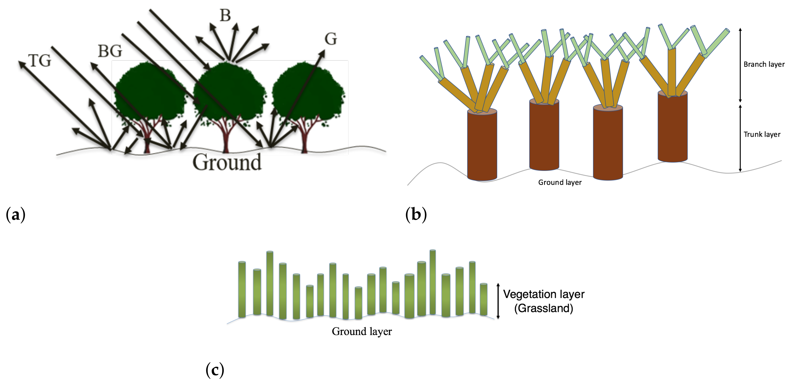
2.1. Direct Ground Bistatic Scattering (G)

In the SSBM, the forest floor is considered to be a dielectric random rough surface. The model by Mironov et al. [30] is used to calculate the dielectric constant of soil from values of soil moisture. The bistatic scattering contribution from a single rough ground surface, with the assumption of flat topography (or zero mean surface), is estimated by the combination of the small perturbation method (SPM) and Kirchhoff approximation (KA). The SPM is used up to second order for estimating the scattering matrix of ground contribution and constructing the direct ground bistatic scattering (G) Stokes matrix M G [29,31]. The zeroth-order SPM solution calculates the scattered field from a smooth flat surface (same as the Fresnel reflection coefficient) and is modified by the KA [29] to include surface roughness. Consequently, the scattering matrix of ground contribution is converted to the ground Stokes matrix M G by Equation (1). The Mueller matrix M ¯ consists of products of the elements of the scattering matrix, and is expressed as
M ¯ = s vv 2 s vh 2 Re s vh * s vv Im s vh * s vv s hv 2 s hh 2 Re s hh * s hv Im s hh * s hv 2 Re s vv s hv * 2 Re s vh s hh * Re s vv s hh * + s hv * s vh Im s vv s hh * s hv * s vh 2 Im s vv s hv * 2 Im s vh s hh * Im s vv s hh * + s hv * s vh Re s vv s hh * s hv * s vh
where s p q is the p q component of the 2-by-2 scattering matrix [32]. The subscripts v and h denote vertical and horizontal polarizations, respectively.

2.2. Vegetation Volume Bistatic Scattering (B)

Bistatic scattering from the vegetation layer on top of the ground surface is estimated by extending the models proposed by [29,31]. Figure 1 presents the vegetation geometry and the three distinct layers (branch layer, trunk layer, and ground layer) used in the SSBM. In this model, trunks are considered finite vertical dielectric cylinders, and the branches are considered randomly oriented dielectric cylinders. For the vegetation volume and double-bounce bistatic scattering contributions, the scattering matrix for an arbitrarily oriented finite dielectric cylinder is first computed and converted to the corresponding Stokes matrix. Then, the Stokes matrix is multiplied by the probability density function (pdf) of cylinder orientation and the density of each element (number of cylinders per squared meter). At last, it averaged over all cylinder orientations. The Stokes matrix of the vegetation layer (branches) M ¯ B , is calculated using [29] (Equation (A18)).

2.3. Branch-Ground (BG) and Trunk-Ground (TG) Double-Bounce Bistatic Scattering

The branch/trunk-ground double-bounce bistatic scattering contribution consists of two paths (Figure 1): (1) transmission through the vegetation layer (branches) and bistatic scattering from the vegetation layer (trunks or branches) in the specular direction, and (2) bistatic scattering from the dielectric rough ground surface and transmission through vegetation layer (branches and trunks) toward the receiver. The ground-branch/trunk double-bounce bistatic scattering contribution is equivalent to branch/trunk-ground double-bounce bistatic scattering contribution. According to [33], the scattering pattern of a vertically oriented finite cylinder resembles a cone. In particular, the scattering pattern of a finite cylinder presents a strong response in the specular direction. The coherent component of the physical optics model, which is based on KA, is used for estimating the bistatic scattering matrix from the ground layer in the double-bounce bistatic scattering contribution. Ultimately, the bistatic scattering matrixes of double-bounce contribution (branch-ground and trunk-ground) are converted to Stokes matrixes M ¯ BG and M ¯ TG , respectively, using Equation (1). The Stokes matrixes, M ¯ BG and M ¯ TG , are integrated over the orientation of branches and trunks, respectively, [27,31].

2.4. Total Bistatic Scattering Stokes Matrix

The bistatic scattering Stokes matrixes of the three scattering mechanisms computed in Section 2.1, Section 2.2 and Section 2.3 are used to determine the total bistatic scattering Stokes matrix of the vegetated land cover M ¯ total . This is accomplished by adding all scattering contributions presented in previous sub-sections, and is expressed as
M ¯ total θ i , ϕ i , θ s , ϕ s = M ¯ B θ i , ϕ i , θ s , ϕ s + T ¯ B θ i , ϕ i T ¯ T θ i , ϕ i M ¯ BG θ i , ϕ i , θ s , ϕ s T ¯ T θ s , ϕ s T ¯ B θ s , ϕ s + T ¯ B θ i , ϕ i T ¯ T θ i , ϕ i M ¯ TG θ i , ϕ i , θ s , ϕ s T ¯ T θ s , ϕ s T ¯ B θ s , ϕ s + T ¯ B θ i , ϕ i T ¯ T θ i , ϕ i M ¯ G θ i , ϕ i , θ s , ϕ s T ¯ T θ s , ϕ s T ¯ B θ s , ϕ s
where incident and scattering paths are denoted as i and s, respectively, and ground, branch, and trunk are expressed as G, B, and T, respectively. Moreover, the T ¯ matrixes present the transmission Stokes matrixes related to the transmission of the wave through vegetation layers (branches and trunks) [33]. Ultimately, for incoherent scattering components, the total bistatic Stokes matrix M ¯ total presented in Equation (2) is converted to co-pol and cross-pol linearly polarized total NBRCS σ total 0 by the method in [32]. Then, the predicted linearly polarized total NBRCS is converted to circularly polarized NBRCS with the method described in Section 3.2. For the coherent scattering component, the total bistatic Stokes matrix M ¯ total is converted to the circularly polarized Fresnel power reflectivity with the method described in Section 3.2.

3. DDM Model

This section discusses the method for calculating the GNSS-R DDM of a flat rough surface in the presence of vegetation using the bistatic scattering model presented in the previous section. The model maps the delay Doppler bins in the DDM to point(s) on the ground surface and calculates the NBRCS of each point. The DDM model can be divided into three parts: (1) estimating the position of the scattering point(s) for each bin of the DDM, (2) calculating the NBRCS for the scattering points, and (3) converting the NBRCS values of the points on the ground surface to a DDM. The details of the first and the last parts are given in the following sub-sections. The second part of the DDM model was presented in Section 2.

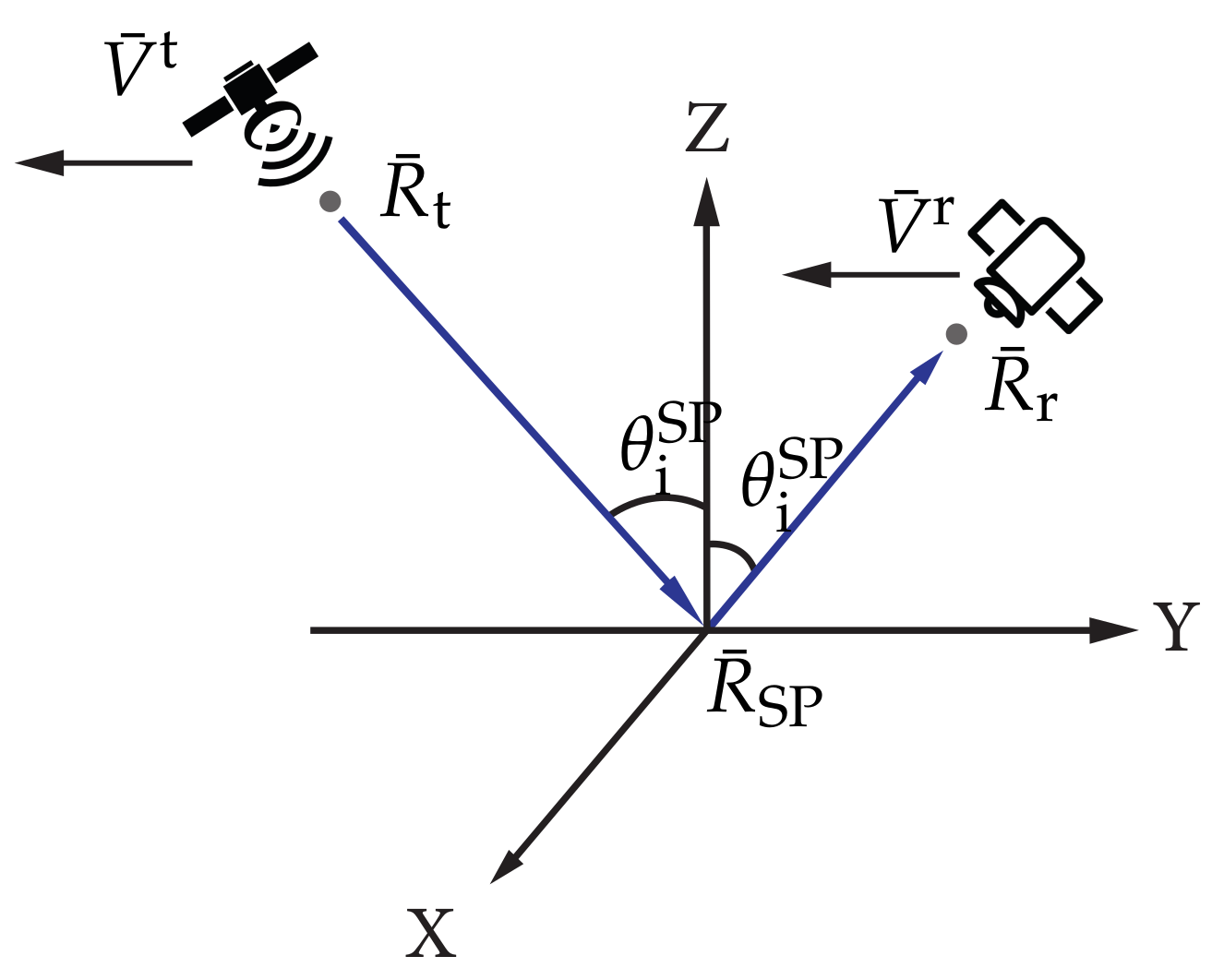
3.1. Estimating the Positions of Scattering Points of a DDM

The model assumes that the ground has a zero mean surface with a small RMS surface roughness and no topography. Furthermore, it assumes the receiver altitude is much lower than the transmitter altitude. This assumption is valid for CYGNSS satellites as their altitude is about 500 k m , while the altitude of the GPS satellites is about 20,200 km. The first assumption simplifies the geometry of the problem. Thus, there exist ellipses on the ground that have constant delays, and parabolas that have constant Doppler frequencies [34,35]. The ellipse of the specular point (SP) delay has both semi-major and semi-minor axes equal to zero, making it a point. Each delay Doppler bin of the DDM corresponds to at most two points on the ground. The geometry of the problem is shown in Figure 2, where the SP position R ¯ SP is the origin, R ¯ t is the transmitter position, R ¯ r is the receiver position, V ¯ t is the velocity of the transmitter, the GPS satellite, V r ¯ is the velocity of the receiver, the CYGNSS satellite, and θ i SP is the incidence angle of the SP. Both R ¯ t and R ¯ r are parallel to the y-axis.
The derivation of the method of estimating the ground positions of each DDM bin and their incidence and scattering angles are presented in Appendix A. These incidence and scattering angles are inputs to the SSBM, which was previously discussed in Section 2.

3.2. Calculating BRCS DDM

The conversion from NBRCS to DDM is performed by first calculating the circularly polarized NBRCS from the linearly polarized NBRCS, given in Section 2. Then using the GPS coarse acquisition (C/A)Woodward ambiguity function (WAF), the left-handed circularly polarized (LHCP) NBRCS is converted to BRCS DDM. The coherent and the incoherent components of the BRCS are calculated individually. The total BRCS DDM is the summation of the two components.
Each CYGNSS delay Doppler mapping instrument (DDMI) contains one right-handed circularly polarized (RHCP) zenith facing navigation antenna and two LHCP nadir looking receiving antennas. The RHCP zenith facing antenna receives GPS signals in the direct path between GPS and CYGNSS satellites, and is used for locating the SP on land and ocean surfaces. Moreover, two LHCP nadir facing antennas are used for GNSS-R. Therefore, in order to use the CYGNSS DDMs for soil moisture retrieval over various land covers, the co-pol (hh and vv) and cross-pol (hv and vh) linearly polarized NBRCS predicted by the forward model, SSBM in Section 2, are converted to LHCP NBRCS σ lr 0 . According to [34], the LHCP NBRCS is expressed as
σ lr 0 = π A s vv + s hh 2 + 2 Im s vh s hv * s vv + s hh + s vh s hv 2
where A is the area, s hh and s vv are the co-pol scattering elements of the total scattering matrix, and s vh and s hv are the cross-pol scattering elements of the total scattering matrix, which are derived from Equations (1) and (2). As the difference between the cross-pol components is much smaller than the co-pol components [31], Equation (3) can be approximated as
σ lr 0 1 4 σ vv 0 + σ hh 0 + 2 Re ρ σ vv 0 σ hh 0
where ρ is defined as
ρ = s vv s hh * s hh 2 s vv 2 .
The numerator and the denominator of Equation (5) are defined as
s vv s hh * = M 33 + M 44 2
s hh 2 s vv 2 = M 22 M 11
where M 11 , M 22 , M 33 and M 44 are the elements of Stokes matrix expressed in Equation(1). In Equation (4), σ hh 0 and σ vv 0 are the co-pol NBRCS estimated by the SSBM. Equation (4) is valid for the incoherent component. For the coherent component, we used the Fresnel power reflectivity Γ lr , as there is no area associated with the coherent component. Equation (4), Equation (1) and the definition of σ 0 [32] (Equations (5.31) and (5.33a)) were used to derive the Fresnel power reflectivity for the coherent component, which is expressed as
Γ coh , lr = 1 4 R rs SP 2 M 11 + M 22 + 2 Re ρ M 22 M 11 .
The subscript lr of σ lr 0 and Γ coh , lr is dropped in the rest of this section, as the conversion from NBRCS or Fresnel power reflectivity to BRCS DDM is general for any polarization.
According to [35], the GPS C/A WAF, with a good approximation, is expressed as
χ δ τ , δ f 2 = Λ δ τ 2 S δ f 2
where Λ δ τ and S δ f are
Λ δ τ = max 0 , 1 δ τ / τ c
S δ f = sinc T i δ f .
In Equations (10) and (11), τ c is the chip length, and T i is the coherent integration period [35]. The approximation of the GPS C/AWAF is good for a relative accuracy of 10 4 [35], which is sufficient for this application. The coherent component of the BRCS DDM σ coh [34] is given as
σ coh i , j = 4 π R rs SP 2 R st SP 2 R rs SP + R st SP 2 Γ coh χ τ i , f j 2
where i and j are the indices of the delay and Doppler bins, respectively, τ i is the relative delay of bin i to the delay of the SP, and f j is the relative Doppler frequency of bin j to the Doppler frequency of the SP. The SP bin is located at i = 0 and j = 0 of the DDM. The incoherent components of the BRCS DDM σ inc [34] are given as
σ inc i , j = σ inc 0 χ τ i τ , f j f D 2 d r
where d r is an integral over the ground surface. τ and f D are the delay and the Doppler, respectively, of the surface relative to the SP. Equation (13) can be simplified using the method given in [34] to
σ inc i , j = σ inc bin i , j A eff i , j
where A eff [ i , j ] is the effective area of σ inc bin [ i , j ] and σ inc bin is defined as
σ inc bin i , j = 1 2 n = 1 , 2 σ inc 0 θ i i , j , n , θ s i , j , n , ϕ i i , j , n , ϕ s i , j , n .
The quantity n in Equation (15) is the index of the ground scattering point for each delay Doppler bin. There is a maximum of two points of the ground for each bin. Thus, σ inc bin is the averaged incoherent NBRCS. Furthermore, in Equation (15), θ i , ϕ i , θ s , and ϕ s are estimated using Equations (A14), (A15), (A16) and (A17), respectively. The effective area of the CYGNSS DDM is provided in the CYGNSS Level 1B (L1B) data, which was used in this implementation. For the SP, the incoherent NBRCS was assumed to be zero as it is negligible compared to the coherent component, as the model assumes the ground surface is flat with small roughness.
The total BRCS DDM can be calculated by adding Equation (14) and Equation (12), which is mathematically expressed as
σ tot i , j = σ inc i , j + σ coh i , j .
The SSBM BRCS DDM is used by the inversion algorithm in the next section to retrieve soil moisture from DDM.

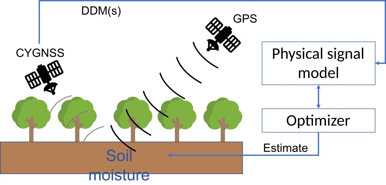
4. Soil Moisture Retrieval Method

CYGNSS L1B science data version 3.1, along with ancillary data, were used to retrieve soil moisture based on a local/global hybrid method that uses multi-directional search and simulated annealing discussed in detail in [28]. In the inverse-scattering problem, this method proved to be substantially faster than the standard simulated annealing method in converging to the global minimum [28]. The physics-based forward model, SSBM DDM in Section 2 and Section 3, was used with parameters from CYGNSS data and ancillary data as inputs to the forward model. The parameters from CYGNSS data were the position and velocity of both the transmitter and the receiver, the position of the SP, the BRCS DDM, and the values of the delay and Doppler of each DDM bins relative to the SP value. These CYGNSS data are used to calculate the incidence and scattering angles of each DDM bin. The ancillary data were divided into vegetation parameters and ground parameters. The vegetation parameters are the dielectric constants, the lengths, the radii, and densities of the three vegetation components, namely, large branches, short branches, and trunks. The ground parameters are soil clay fraction, correlation length of the random rough surface, and RMS surface roughness σ h . The ratio of correlation length to RMS surface roughness was assumed to be 10 [36].
This method retrieves soil moisture with the native spatial and temporal resolution of the measurement. In GNSS-R, the spatial resolution depends on the position of both the transmitter and the receiver relative to the ground surface. Furthermore, both the spatial and the temporal resolutions depend on the incoherent averaging of the DDM. For CYGNSS, the incoherent averaging time for normal operation was one second, but it was switched to half a second in late 2019. Additionally, the topography of the ground affects the spatial resolution. Smoother surfaces tend to give finer resolution. The approximate upper and lower limits of the spatial resolution of the DDMs used in this study are discussed in Section 6.2.
Two schemes were used in retrieving soil moisture from CYGNSS DDMs. The first scheme assumes that the RMS surface roughness is known and only retrieves soil moisture. Figure 3a shows the flowchart of the first retrieval scheme. The second scheme retrieves soil moisture and RMS surface roughness simultaneously. Surface roughness measurements are generally scarce. Even when surface roughness data are collected during field campaigns, their spatial coverage is limited and may not represent the equivalent RMS surface roughness of the area covered by a given DDM, which is typically several km 2 . Therefore, if successful, the second scheme is advantageous because it treats surface roughness as an unknown and retrieves it along with the soil moisture. The flowchart of the second retrieval scheme is presented in Figure 3b. Both schemes can use either a single DDM or multiple DDMs.
At first, a single DDM was used to retrieve soil moisture using both schemes. In addition, in the case of the second scheme, the use of two DDMs with the same area but different incidence angles was investigated with simulated DDMs. The two DDMs were selected such that they had nearly equal soil moisture values. Thus, two independent measurements were used to retrieve two geophysical parameters.
In the retrieval algorithm, the dynamic range of soil moisture was between 0.01 and 0.6 m 3 m 3 , and the allowed range of RMS surface roughness was between 0.5 and 2.5 cm. This choice was based on the expected terrain surface roughness and the SSBM validity limit. The algorithm does not use the entire CYGNSS DDM; instead, it uses a subset of the DDM consisting of three delay and five Doppler bins centered at SP. These bins are used to calculate an averaged NBRCS. The method of calculating the averaged NBRCS is similar to the method used by the CYGNSS processor [18], which is expressed as
σ 0 = i = 0 2 j = 2 2 σ i , j i = 0 2 j = 2 2 A i , j
where σ is the BRCS, and A is the bin area in units of m 2 . The numbers i and j are the delay and Doppler bin indices, respectively, relative to the SP. The SP is at i = 0 and j = 0 , which is the reported index in CYGNSS data. The forward model DDM, described in Section 3, was used to construct the DDM and then estimate the averaged NBRCS σ 0 .
The relationship between soil moisture and σ 0 is not always linear. However, if all the other parameters are fixed, the relationship is linear, as shown in Figure 4. The level of sensitivity to soil moisture depends on the other parameters of the forward model.
The tuning parameters of the multidirectional-search-based simulated annealing algorithm [28] are N m d , N s , N t , N, l step , and f stop . The parameters N m d , N s , and N t are the maximum number of iterations of the algorithm inner searches. The number of iterations is N. The parameter l step is the step limit in the multidirectional search. The algorithm stops if the cost function f cos t is less or equal f stop or the number of iterations reached N. The parameters and the algorithm were discussed in [28].
The cost function is defined as
f cost = i = 1 n σ measured 0 [ i ] σ forward 0 [ i ] σ measured 0 [ i ] 2
where n is the number of DDMs. The subscript ‘measured’ represents the measured σ 0 (CYGNSS or simulation) while the subscript ‘forward’ represents the value of σ 0 calculated from SSBM.

5. Simulation Setup and Validation Site

To validate the proposed retrieval algorithm, we used both simulated DDMs and CYGNSSs DDM to retrieve soil moisture and compare with in situ measurements. For the simulation experiment, the Monte Carlo technique was used to estimate the performance of the retrieval algorithm. The simulation setup and the validation site are discussed in detail in the following sections.

5.1. Simulation Setup

We used the retrieval algorithm discussed in Section 4 to retrieve soil moisture from simulated DDMs. The simulated DDMs were generated using the SSBM with additive zero mean white Gaussian noise. The additive noise accounts mainly for the receiver noise. The random noise samples were added to each DDM bin. The signal-to-noise ratio (SNR) in this simulation was the ratio of the SP bin power to the noise power. The population size of the Monte Carlo simulation was 10.

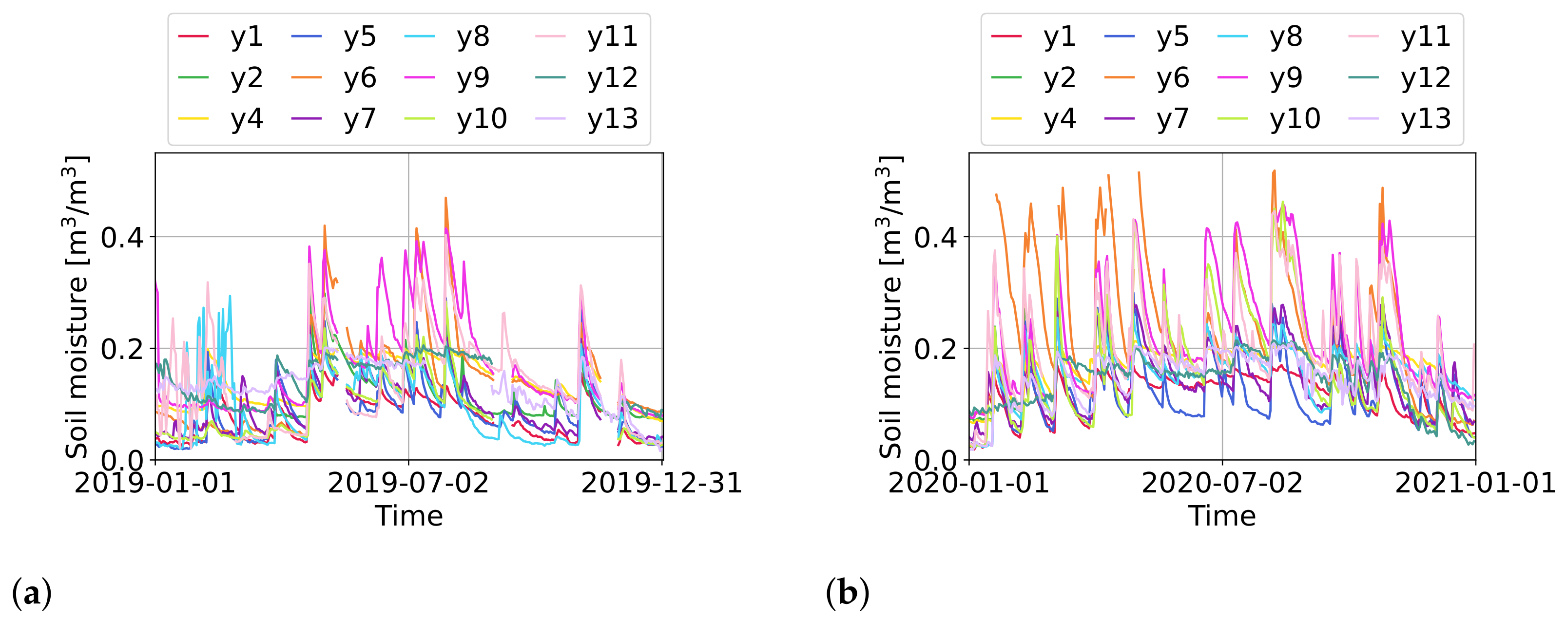
5.2. Validation Site

The SMAP Yanco region was selected for validating the retrieval algorithm. This site was chosen since it (1) has negligible topography, (2) has active in situ soil moisture sensors, and (3) is located within the CYGNSS coverage area. The Yanco region is located in the southeast of Australia. It is a flat area of 2500 k m 2 , which includes 13 sites with in situ soil measurement sensors [37]. Figure 5 shows a photo of the validation site. The sensors installed at Yanco sites measure surface soil moisture (0–5 cm) and soil temperature at three depths (1, 2.5 and 5 cm) [37]. Moreover, according to [37], the median root zone 0–90 cm moisture content of Yanco region sensors (Y1–Y13) from 2004 to 2010 is 0.186–0.33 m 3 m 3 . We selected the data from the years 2019 and 2020 for validation, as both CYGNSS and the in situ sensors have available data in these year. Most of the sensors were operational in this time period. Figure 6 shows the daily average of the in situ surface soil moisture values of the sensors for the entire years of 2019 and 2020. The in situ soil moisture values of all of the sensors were between 0.005 m 3 m 3 and 0.522 m 3 m 3 , for the year 2019. For 2020, the in situ soil moisture values were between 0.002 m 3 m 3 and 0.544 m 3 m 3 , which is similar to the previous year.
According to [37], the Yanco region is covered by mostly improved pasture with minimal woody vegetation, which falls under the grassland International Geosphere-Biosphere Programme (IGBP) land cover type. The region is used mainly for grazing and crops. The soil clay content is between 11% and 25% in the region.
The majority of the sensors have similar measured soil moisture readings over the year of 2019, as illustrated in Figure 6. The measurements of the Y8 sensor were used for the validation, as they represent the soil moisture values at the site. The sensor is located at S 34.84697° E 146.41398°, with ground elevation of 149 m . The soil clay content is 11.7% for the nearest soil texture measurement to the sensor [38]. The in situ soil moisture measurements of the Y8 sensor were between 0.016% and 0.351 m 3 m 3 , as shown in Figure 6.

6. Results

In this section, the results of both the simulation and the validation experiments are presented. We used the retrieval algorithm of Section 4 and the SSBM DDM of Section 3 to retrieve soil moisture from DDMs. Two types of vegetation were used in the simulation: grassland and mixed forest, which are classes 5 and 10, respectively, of the IGBP land cover classification system. For validation, CYGNSS L1B data, which include BRCS DDMs, were used to retrieve soil moisture. The retrieved soil moisture values were compared to the in situ soil moisture at the Yanco validation site. The same tuning parameters of the retrieval algorithm were used in simulations and validations. The metrics for the soil moisture retrievals are RMS error (RMSE), unbiased RMSE (ubRMSE), and the correlation coefficient r. These were calculated according to Entekhabi et al. [39].

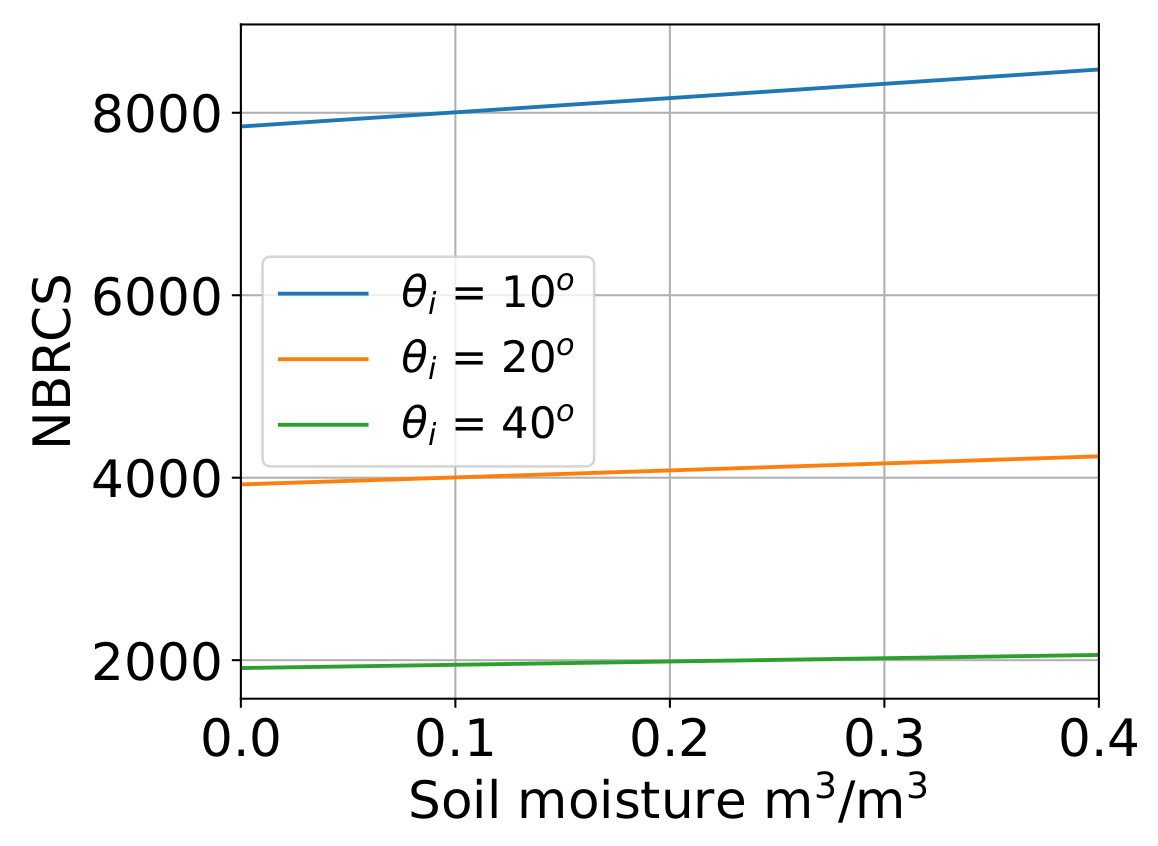
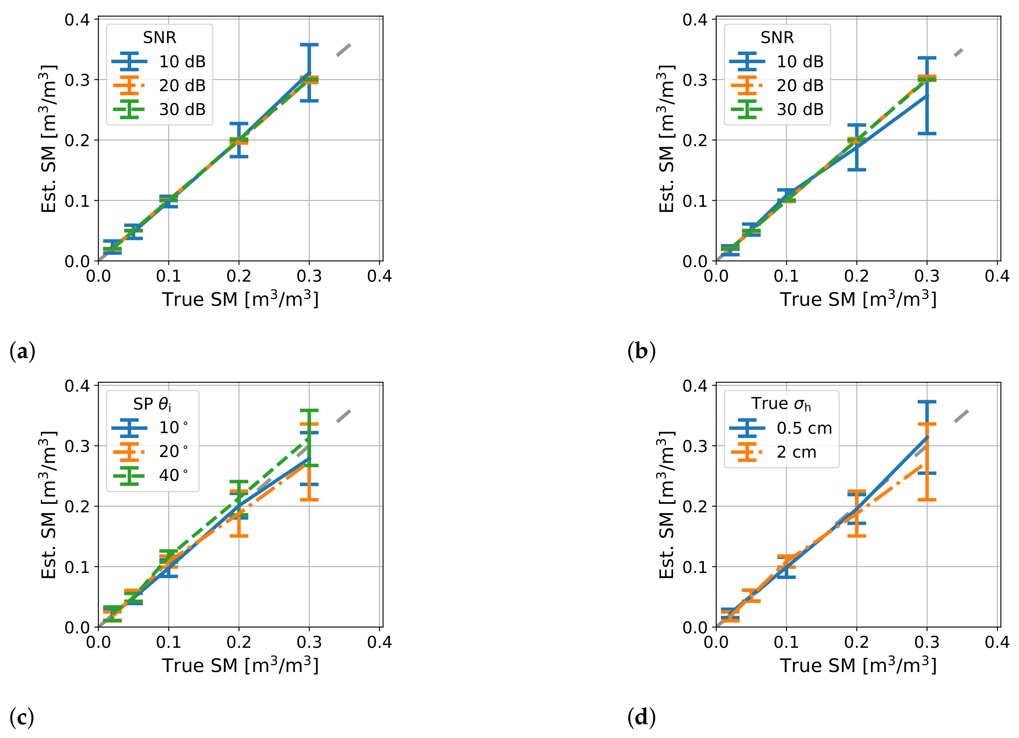
6.1. Simulation Results

The simulated DDMs were generated by varying several parameters, which include the incidence angle of the SP, soil moisture, surface roughness, SNR, and vegetation. The soil moisture values were 0.02, 0.05, 0.1, 0.2 and 0.3 m 3 m 3 . These values cover the dry to the half saturation range of soil moisture. Two values of RMS surface roughness σ h were used in the simulation, those being 0.5 and 2.0 cm. The 2 cm RMS surface roughness value is above the validity limit of SPM. However, this does not have a significant impact on the DDM, as the contribution of the noncoherent scattering components (SPM) is small compared to the contribution of the coherent scattering components (KA). The SNR values were 10, 20 and 30 dB. The lower bound of SNR values was selected to be the same as the lower SNR values for the selected CYGNSS DDMs of the Yanco validation site. The surface correlation length was set to be 10 times the RMS surface roughness value. The clay percentage was set to 11.7 %, which is the same value used in the validation experiments. For the single DDM retrievals, the SP incidence angles were 10°, 20° and 40°. The selected incidence angles cover the range of values observed in the CYGNSS DDMs over the Yanco validation site. Furthermore, the incidence angle of SMAP is about 40° [1]. For the two-DDM retrieval, 10° and 40° SP incidence angles were used. The tuning parameters of the retrieval algorithm N m d , N s , N t , N, presented in Section 3, were 10, 5, 5 and 30, respectively. The step limit l step was 10−4, and f stop was 10−2. The values of the tuning parameters were selected based on empirical trials. The vegetation parameters of the two vegetation types are shown in Table 1. The vegetation water content (VWC) is not an input to the model. However, it was presented to help understand the above ground biomass. The mixed forest vegetation parameters were from the Canadian Experiment for Soil Moisture in 2010 (CanEx-SM10) [40] while the parameters of grassland were from AirMOSS field campaign [41]. These parameters were used in soil moisture retrieval from active radars [4,40]. We did not simulate all of the combinations of geophysical parameters as the numerical simulations are computationally expensive.

6.1.1. Retrievals from a Single DDM

Using the first retrieval scheme, we observed that the retrieval algorithm has a negligible estimation bias. Moreover, the RMSE was proportional to the SNR, as expected. Specifically, for the first scheme with grassland vegetation cover, the RMSEs were 0.031, 0.003 and 0.0003 m 3 m 3 for SNR of 10, 20 and 30 dB, respectively. Furthermore, the correlation coefficient r was over 0.95, and it was proportional to the SNR. Figure 7 shows the performance of the first retrieval scheme with the simulated DDMs of grassland land cover, with different values of SNR, SP incidence angle, and RMS surface roughness. The error bars in Figure 7 represent one standard deviation from the mean. Figure 7a,b show the performance with various SNR values; Figure 7a is for RMS surface roughness of 0.5 cm and SP incidence angle of 10°, while Figure 7b is for RMS surface roughness of 2 cm and SP incidence angle of 20°. Furthermore, Figure 7c,d show the performance for 10 dB SNR, with different values of SP incidence angles and RMS surface roughness, respectively.
The performance of the first retrieval scheme of mixed forest land cover was very similar to the retrieval of grassland land cover, as shown in Figure 8a,b. The mixed forest land cover had a positive estimation bias, while the grassland had a negative estimation bias; both of them were insignificant compared to the true soil moisture value. The bias was proportional to the soil moisture value, as shown in Figure 8a,b.
Soil moisture retrieval using the second scheme had a weaker performance compared to the first scheme. For SP incidence angle of 20° and surface roughness of 2 cm, the retrieval from grassland had an ubRMSE of 0.259 and 0.253 m 3 m 3 for SNR of 10 and 20 dB, respectively. For mixed forest land cover, with the same values of other parameters, the ubRMSE was 0.135 and 0.128 m 3 m 3 for SNR of 10 and 20 dB, respectively. Figure 8c,d and Figure 9a,b show these results. The retrieval from grassland DDMs had a higher bias, compared to those from mixed forest DDMs, which had a low bias. Specifically, the biases of the retrievals from mixed forest DDMs were 0.008, 0.011, 0.026, 0.058 and 0.117 m 3 m 3 for soil moisture of 0.02, 0.05, 0.1, 0.2 and 0.3 m 3 m 3 . The retrievals from mixed forest DDMs had an overall correlation coefficient r of 0.74. However, the retrievals from grassland DDM had a correlation coefficient r close to 0.4. The case of mixed forest with surface roughness of 2 cm and incidence angle of 10° had high RMSE and estimation bias, as shown in Figure 9b. The rest of the mixed forest land cover simulations had a negligible estimation bias, an ubRMSE of less than 0.04 m 3 m 3 , and a correlation factor r of over 0.95. Figure 9c,d show both the retrieved soil moisture and surface roughness values using the second retrieval scheme with different SP incidence angles. The retrieval algorithm underestimated the surface roughness of the mixed forest land cover, while the estimation was close to the true value for the grassland land cover. However, it had a large variance, as shown in Figure 9c.

6.1.2. Retrievals from Two DDMs

Solving the inverse problem of two unknowns from a single measurement is ill posed. To address this issue in the second retrieval scheme, the next step is to use two DDMs in the retrieval.
To understand the retrieval algorithm behavior with different values of soil moisture and surface roughness, the cost function needs to be analyzed. Figure 10 shows the cost functions for DDMs of 10° and 40° SP incidence angles with different values of soil moisture, surface roughness, and land cover types. Figure 10a,d show the cost function of grassland land cover type, while Figure 10e,h show the cost function of mixed forest land cover type. The minimum value of the cost function is zero, and it is when both soil moisture and surface roughness are recovered exactly; the location is shown by the purple dot in Figure 10. The gray dot in Figure 10 shows the minimum value in the plot. Ideally, the purple and the gray dots should be coincident. However, depending on the shape of some cost functions, the dots could be far from each other. Figure 10a is an example of this effect. The cost function is very sensitive to surface roughness, as shown in Figure 10a,b,e,f. The cost function of grassland land cover type is generally flatter than the cost function of mixed forest land cover type. Retrievals from forest land cover are therefore expected to reach a convergent solution faster and more accurately, as the gradient of the cost function is better defined. Furthermore, in some cases, there exists a trench of low cost function values that passes through the true parameters, resulting in ambiguous solutions. This effect can be clearly observed in Figure 10c.
We performed a Monte Carlo simulation for DDMs with incidence angles 10° and 40° only. The SNR values were 10 dB and 20 dB. The other parameters were the same as in Section 6.1.1. The Monte Carlo simulation results of retrieving both soil moisture and surface roughness from two DDMs are shown in Figure 11. As expected from cost function graphs, the retrievals from the mixed forest land cover DDMs outperformed the retrievals from grassland land cover DDMs, as illustrated in Figure 11a,d. More explanation will be provided later in Section 7. For grassland land cover type, the retrievals of 2 cm surface roughness had better accuracy for low soil moisture values compared to the retrievals of 0.5 cm surface roughness. However, for high soil moisture values, the retrievals of 0.5 cm surface roughness outperformed the retrievals of 2 cm surface roughness, as shown in Figure 11a,b. The soil moisture retrieval performance from grassland land cover DDMs was significantly impacted by noise, as shown in Figure 11e,f. The retrievals, of grassland land cover, for the case of 10 dB SNR had an ubRMSE of 0.15   m 3 m 3 , while the retrievals of 20 dB SNR had an ubRMSE of 0.08   m 3 m 3 . The correlation factor was 0.67 for 10 dB SNR and 0.76 for 20 dB SNR. The bias was 0.08   m 3 m 3 for 10 dB SNR and 0.02   m 3 m 3 for 20 dB SNR. The retrievals in the case of mixed forest land cover had superior performance. The ubRMSE for SNR of 10 dB and 20 dB was 0.02   m 3 m 3 and 0.002   m 3 m 3 , respectively. The correlation factor was greater than 0.98, and the bias was less than 0.01   m 3 m 3 .

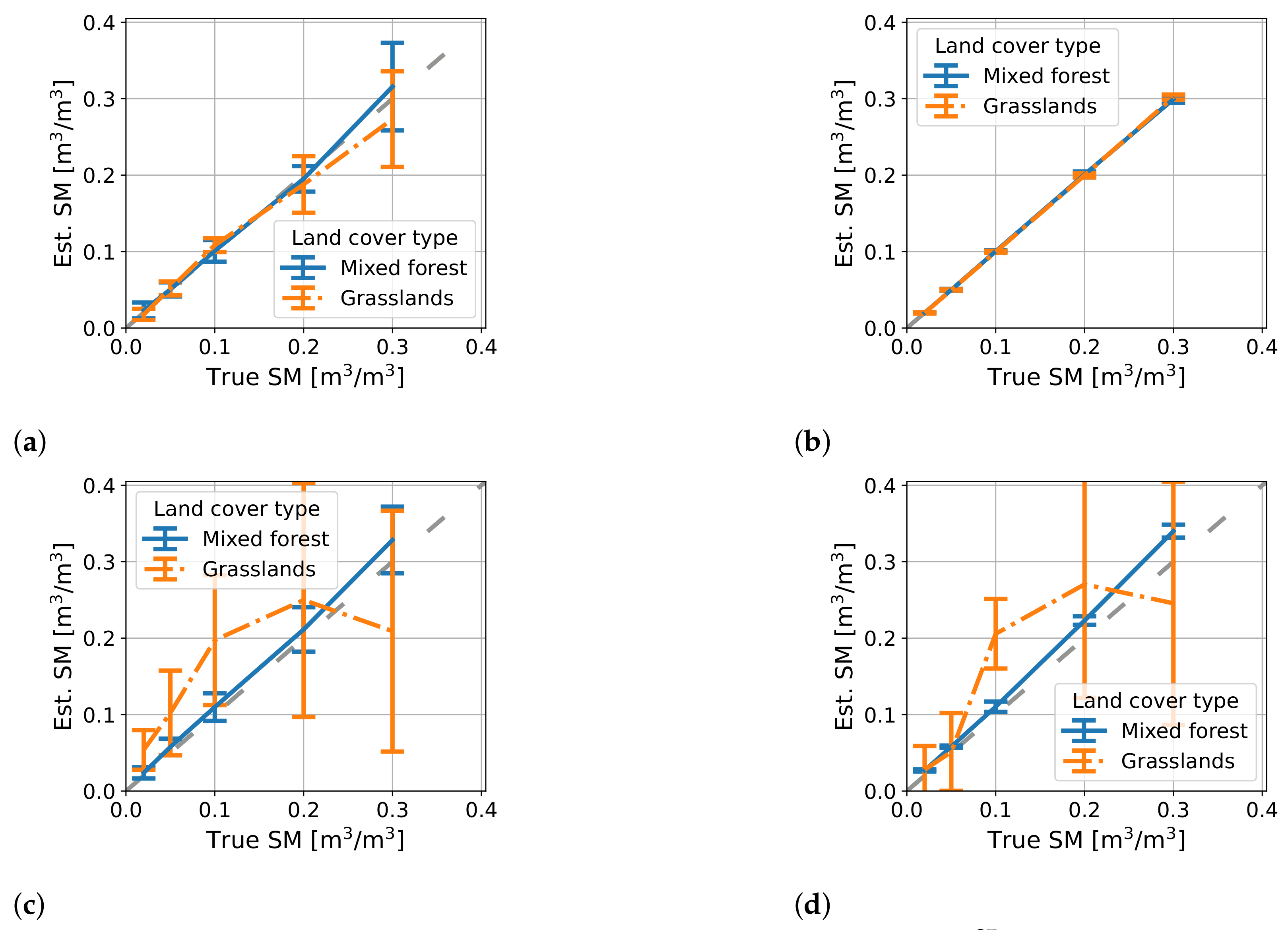
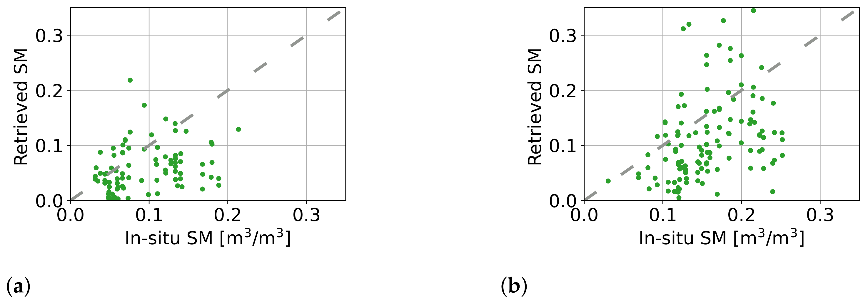
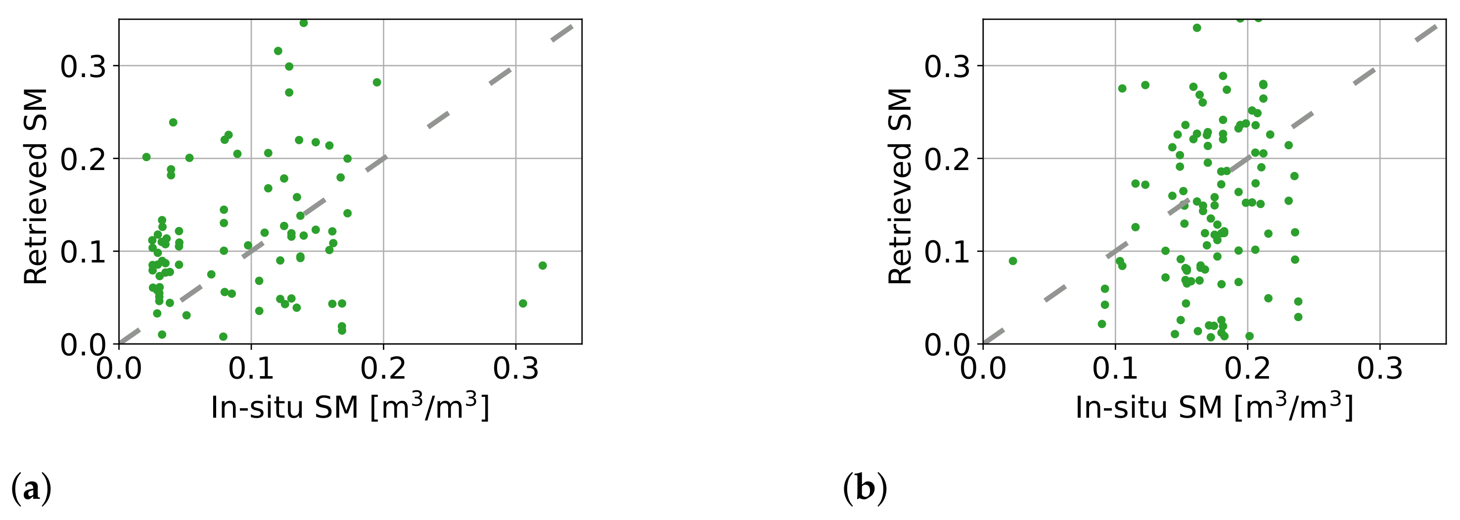
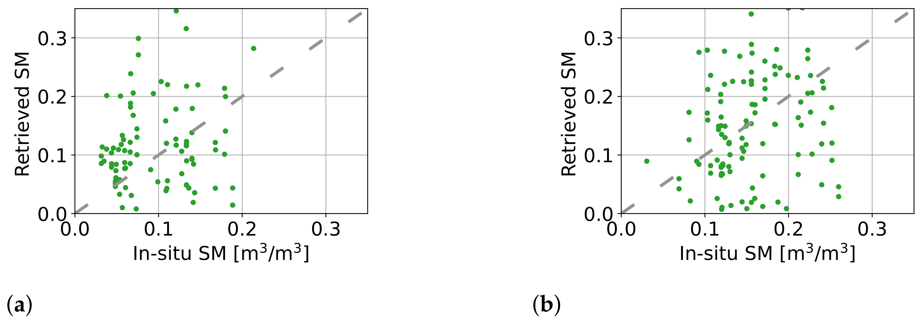
6.2. Validation Results

The inversion algorithm presented in Section 4 and the SSBM DDM of Section 3 were used to retrieve soil moisture from CYGNSS L1B version 3.1 data for 2019 over the validation site. More details of the validation site were given in Section 5.2. Both of the single-DDM retrieval schemes were used to retrieve soil moisture from 96 CYGNSS DDMs. The SP locations of the DDMs are within 5 km of the sensor location and have reported SNR values of over 10 dB. Moreover, in selecting the DDMs, we discarded any data with quality flags that indicate issues in the CYGNSS measurements. Specifically, data with attitude errors, abnormality in the hardware, or a reported negative antenna gain at the SP location were discarded. The criteria of selecting CYGNSS data were similar to the criteria reported in other soil moisture retrieval methods using CYGNSS data [20,21]. We used the grassland vegetation parameters presented in Table 1 in the inversion algorithm. Furthermore, the soil clay percentage is 11.7 %, which is the reported clay percentage of the nearest location to the in situ sensors [38]. The tuning parameters of the retrieval algorithm were the same as the values used in the simulations.
Figure 12 shows one example of BRCS DDM observed by CYGNSS and the corresponding simulated DDM using SSBM. The CYGNSS DDM was collected on 2019-10-09 20:40:00 UTC by spacecraft number one and channel two. The SP incidence angle was 22°, and the reported SP location was −34.8054° latitude and 146.3956° longitude. The forward model was generated with an RMS surface roughness of 2 cm and a soil moisture value of 0.025   m 3 m 3 , derived from Yanco in situ soil moisture measurements. For the retrievals, a subset of the DDM is used, as discussed in Section 4. In Figure 12, the full DDM is shown with 17 delay bins and 11 Doppler bins.
The ground positions of each delay Doppler bin, within the 3 × 5 box, are shown in Figure 13 along with the in situ sensors location. The positions of the delay Doppler bins were calculated using the method presented in Section 3.1. The map shows that there are two locations for each bin except the SP bin. The approximate resolution of this DDM is between 17 km and 32 km. The lower limit is the first Fresnel zone, and the upper limit is the maximum distance between two points in the area of the selected 3 × 5 box of the DDM.
The in situ soil moisture and the NBRCS of the selected DDMs in this study are shown in Figure 14. The plotted NBRCS values of SSBM were calculated using the in situ soil moisture values. The figure shows that the averaged in situ soil moisture value of the selected points in the year 2020 is higher than the value of 2019.
About 250 CYGNSS DDMs in 2019 and 2020 were used in the retrieval. Their approximate native spatial resolution is between 10 km and 50 km. The lower limit was calculated using the maximum distance between two points in the first Fresnel zone, while the upper limit was calculated using the maximum distance between two points within the area covered by the 3 × 5 subset of the DDM. The results of the soil moisture retrievals using the two schemes are given in the following sub-sections.

6.2.1. Results of First Retrieval Scheme: Soil Moisture Is the Only Unknown

The first retrieval scheme, as discussed in Section 4, considers the RMS surface roughness as a known parameter and the soil moisture as an unknown. The RMS surface roughness was set to 2 cm, and accordingly, the surface correlation length was set to 20 cm. The value was selected empirically, as we do not have local RMS surface roughness measurements. The results of the second retrieval scheme were used in aiding the selection of the value. We discarded the retrievals that were nonphysical or had soil moisture value above the saturation level. A retrieval is discarded if the retrieved soil moisture value is greater than 0.5   m 3 m 3 or less than 0.0025   m 3 m 3 . The upper limit value for the retrieved soil moisture was set to 0.5   m 3 m 3 as this can be considered saturated soil and we do not expect the soil moisture to reach this value in this region. For the first retrieval scheme, 37 out of the 250 retrievals were discarded. Figure 15a shows the in situ soil moisture of station Y8 versus the retrieved soil moisture values. For 2019, the retrieved values had an RMSE of 0.074   m 3 m 3 , an ubRMSE of 0.069   m 3 m 3 , and a correlation coefficient r of 0.28. Retrievals from DDMs of 2019 has higher performance than retrievals form DDMs of 2020.
The retrieved soil moisture values were compared to the averaged soil moisture values of Three in situ soil moisture stations, as shown in Figure 16. The first station was Y8. The rest were Y5 and Y7, which are the closest stations to the Y8 station. The averaging of the in situ soil moisture values was to reduce the sensors noise, and reduce the effect of outliers. The retrieval performance was higher than using only the in situ data of only the Y8 station as the true soil moisture. Using the averaged in situ soil moisture values had an RMSE of 0.068   m 3 m 3 , an ubRMSE of 0.060   m 3 m 3 , and a correlation coefficient r of 0.26, for the retrievals from 2019 DDMs. For 2020 DDMs, the RMSE was 0.098   m 3 m 3 , the ubRMSE was 0.091   m 3 m 3 , and the correlation coefficient r was 0.21.

6.2.2. Results of Second Retrieval Scheme: Both Soil Moisture and Surface Roughness Are Unknowns

The second retrieval scheme, discussed in Section 4, considers both the RMS surface roughness and the soil moisture as unknowns. Similar to the first scheme, presented in Section 6.2.1, the vegetation parameters presented in Table 1 and the same soil clay percentage were used in the retrieval algorithm. The surface correlation length was set to 10 times the RMS surface roughness. Furthermore, similar to the first scheme, the nonphysical or had soil moisture value above the saturation level retrieved soil moisture values were discarded, using the same criteria. 35 out of 250 retrievals were discarded.
Figure 17 shows the in situ soil moisture values of station Y8 versus the retrieved soil moisture values. For 2019 DDM, the retrieved soil moisture values had an RMSE of 0.096   m 3 m 3 , ubRMSE of 0.091   m 3 m 3 , and a correlation coefficient r of 0.15. For the retrievals from the DDMs of 2020, the RMSE was 0.116   m 3 m 3 , the ubRMSE was 0.116   m 3 m 3 , and the correlation factor r was 0.21.
Similar to the first scheme results, the retrieved soil moisture values were compared to the averaged soil moisture values of Y5, Y7, and Y8 stations, as shown in Figure 18. Unlike the findings of the first scheme, using the averaged in situ soil moisture did not enhance the retrievals for all the years. For 2019 retrievals, the performance metrics were enhanced. However, the opposite was for the retrievals from 2020 DDMs; the performance metrics using the averaged in situ soil moisture value were declined. For the retrievals from the 2019 DDMs, the RMSE was 0.088   m 3 m 3 , the ubRMSE was 0.085   m 3 m 3 , and the correlation factor r was 0.15. The retrievals from the 2020 DDMs had an RMSE of 0.12   m 3 m 3 , an ubRMSE of 0.118   m 3 m 3 , and a correlation factor r of 0.21.
The performance metrics of both retrieval schemes for both 2019 and 2020 DDMs are summarized in Table 2. The in situ sensors column has the name of the sensors that their measurements used in calculating the performance metrics.

7. Discussion

The BRCS DDM predicted by the SSBM and the BRCS DDM provided by the L1B CYGNSS data for SMAP Yanco sites were presented in Section 6. Figure 12 illustrated the SSBM DDM constructed with the method expressed in Section 3. Furthermore, Figure 12 showed that the structure and shape of the DDM predicted by the forward model were in good agreement with the CYGNSS DDM, with some differences: (1) the data seem to be a blurred version of the model in the near specular bins, suggesting that SSBM lacks near-specular resolution, which makes sense because we effectively modeled the NBRCS as a sum of a Dirac delta function (coherent Kirchhoff) and a relatively smooth function (SPM), whereas we know that NBRCS actually behaves more like a Gaussian function, which has a blurring effect, (2) the model overestimates the more diffuse scattering at larger delays, and (3) the SSBM DDM is symmetric around the zero Doppler line, whereas the CYGNSS DDM is not symmetric. The last two points are mainly because the model assumes no topography. However, these differences have minimal impact on the retrievals, as we used the averaged NBRCS, Equation (17), which uses a 3 × 5 portion of the full DDM.
The BRCS value of the SP and the averaged NBRCS of some of the CYGNSS DDMs had some differences with the ones generated by the SSBM. Some of these discrepancies are related to either error in the validity of the assumptions in the model (such as having a perfectly flat surface) or its input parameters. However, there were some calibration errors related to CYGNSS DDMs over land. Most of these errors were resolved in the data version used in this study. Modeling the DDM can point out these calibration/signal processing related issues in CYGNSS data and assist in resolving them.
The inversion algorithm includes the SSBM, discussed in Section 2, and the hybrid local/global optimization method [28]. In Section 6, two soil moisture retrieval schemes using a single DDM were used to retrieve soil moisture from both simulated and CYGNSS DDMs. Furthermore, soil moisture and surface roughness values were retrieved using two simulated DDMs with different incidence angles. In the first scheme, presented in Section 6.2.1, the surface roughness was known, and the soil moisture (at 0–5 cm) was unknown. The second scheme of soil moisture retrieval, presented in Section 6.2.2, considered both surface roughness and soil moisture as unknowns. The two-DDM scheme is similar to the second scheme in that it retrieves both surface roughness and soil moisture, but it uses two DDMs to retrieve these two unknowns.
For retrievals from simulated DDMs, the first retrieval scheme had better performance compared to the second retrieval scheme. This was expected as the first scheme retrieved a single geophysical parameter, soil moisture, while the second scheme retrieved two geophysical parameters, soil moisture and surface roughness, from a single DDM. The second retrieval scheme is therefore inherently ill posed. We observed that the simulated DDMs of grassland land cover are more sensitive to the error in surface roughness estimation compared to the mixed forest land cover, as illustrated in Figure 9c,d. The case of the second retrieval method with mixed forest land cover, 2 cm surface roughness, and 10° incidence angle was an outlier compared to the other results with the same land cover type. This was expected from the cost function shape for this specific case. The retrieval performance of the second scheme for the simulated mixed forest case is very close to the performance of the retrievals using the first scheme, with the exception of the outlier case. The soil moisture retrievals from the simulated DDMs using the first retrieval scheme of both grassland and mixed forest land covers had an ubRMSE below 0.04   m 3 m 3 with a correlation coefficient r over 0.95. The ubRMSE was proportional to the true soil moisture and it was lower than 0.04   m 3 m 3 . The results of the simulations, except for the case of grassland land cover using the second retrievals scheme, are encouraging for considering DDMs with SNR lower than 10 dB. Decreasing the SNR requirements will increase the ubRMSE.
The two-DDM cost function analysis showed the difficulty of the retrieval from an optimization point of view, especially for the case of grassland land cover. The areas with small gradient values neighboring the global minimum in the cost function pose a challenge to the retrieval algorithm, as this may require a large number of iterations to reach the global minimum. The Monte Carlo simulation of retrieving soil moisture from two DDMs showed that this approach increased the accuracy of the retrieval.
In the retrievals from CYGNSS DDMs in 2019, the ubRMSE was about 0.09   m 3 m 3 for the second retrieval scheme and less than 0.06   m 3 m 3 for the first retrieval scheme. The retrieval performance was lower for the DDM of 2020; the ubRMSE increased by about 0.03   m 3 m 3 . This is expected as the in situ soil moisture values were higher in 2020 compared to the values of 2019, as shown in Figure 4. The bias of all retrievals was small, below 0.04   m 3 m 3 . The error variance was proportional to the in situ soil moisture values, as illustrated in Figure 16a and Figure 18a. This is consistent with the simulation findings. Both retrievals had a low correlation coefficient r. The first scheme performed better than the second scheme in all merits, which is similar to the simulation results.
The spatial averaging of soil moisture values of multiple in situ sensors reduced the measurement noise and made the value more robust to outliers. This was the expected reason for getting better performance metrics, for most of the retrievals, compared to the soil moisture values of only the Y8 sensor, as shown in Table 2. As mentioned in the previous section, the performance metrics of all the retrievals improved with the use of spatially averaged in situ soil moisture values, except the retrievals from 2020 DDMs using the second scheme. The performance of these retrievals slightly decreased. The bias increased by 0.015   m 3 m 3 , and the rest of the metrics had insignificant changes.
The surface roughness parameter in the forward model can be used in addition to its original purpose as a tuning parameter to account for the discrepancies between the forward model DDM and the CYGNSS DDM. Thus, the retrieval algorithm can mitigate some CYGNSS DDM calibration issues.
As noted earlier in this section, the second scheme suffers from being ill posed, as the algorithm retrieves two parameters from a single DDM. Thus, the inverse problem is underdetermined. Generally, the first scheme performance depends heavily on the selected values of RMS surface roughness, which is often times not available.
Previous soil moisture products from CYGNSS have reported ubRMSE metrics around 0.05   m 3 m 3 . Specifically, Chew et al. [20] reported a median ubRMSE of 0.049   m 3 m 3 , Senyurek et al. [21] reported a minimum ubRMSE of 0.052   m 3 m 3 using all data for training and 0.049   m 3 m 3 using site-specific training. Al-Khaldi et al. reported RMSE of 0.045   m 3 m 3 over variant terrains compared to SMAP soil moisture product. For comparison with in situ soil moisture, the RMSE value was 0.071   m 3 m 3 , and the ubRMSE value was 0.067   m 3 m 3 for the Yanco site, the same site used for validation of the method presented in this paper. The ubRMSE of the retrievals from 2019 DDMs using the first scheme in paper was close to the values reported in the literature [23]. However, retrievals from 2020 DDMs had a higher ubRMSE value compared to the retrievals in the literature.
The factors that contribute to the errors in our physics-based model predictions are listed as follows:
  • The footprint of CYGNSS DDM is large, but the in situ soil moisture sensors cover a small region of the foot-print. Thus, the average soil moisture value, which is observed by the CYGNSS DDM, could be different from the in situ soil moisture values.
  • Any possible variations in vegetation land cover over the course of the year resulting in variations in the vegetation input parameters, which potentially lead to errors in the SSBM predictions.
  • Calibration issues in CYGNSS data.
  • Modeling errors, which include the lack of considering topography and multi ground layers, potentially lead to less accurate results.
The retrieval algorithm can be used as a basis for more advanced retrieval algorithms. Improving the accuracy of the forward model improves the retrieval performance. One way of advancing the forward model is to integrate the SSBM presented in this paper with the DDM model proposed in [43] to extend the model for heterogeneous surfaces and topography. Furthermore, we believe the simultaneous retrieval of both soil moisture and surface roughness from multiple DDMs is the path forward to increase the performance of physics-based retrieval methods and reduces the dependence on ancillary data layers. To address the flatness problem of the cost function in some cases, which causes lack of sensitivity to the unknowns, a study of other options for the cost function is needed.

8. Conclusions

This paper presented a retrieval approach using a physics-based bistatic scattering forward model, the SSBM, for soil moisture estimation from GNSS-reflected signals over various vegetated land covers. The majority of the previous soil moisture retrieval methods from CYGNSS DDMs used empirical or regression-based methods for soil moisture retrieval. The physics-based method of this paper incorporates physical insight into the retrieval, which allows for a systematic approach without depending on potentially faulty or an incomplete training/fitting data set. Furthermore, the method does not depend on other soil moisture products, such as SMAP. However, physics-based methods are bounded by the forward model accuracy and sensitive to calibration errors in the measured data. The methods of this paper were tested on both simulated DDMs and measured CYGNSS DDMs (version 3.1). The simulated DDMs were for grassland (VWC of 0.19   kg m 2 ) and mixed forest (VWC of 4.89   kg m 2 ) IGBP land cover types. The CYGNSS DDMs were observed over the SMAP Yanco site that has the IGBP grassland land cover class. Retrievals were accomplished using a single DDM and two DDMs. For the single DDM retrieval two schemes were proposed. In the first scheme, the retrieval was performed with the assumption that RMS surface roughness is a known parameter and soil moisture is unknown. In the second scheme, both soil moisture and RMS surface roughness were considered unknowns. The retrieval from two DDMs was implemented similar to the second scheme, except the use of two DDMs with different incidence angles.
The results of the retrievals from a single simulated DDM using the first retrieval scheme showed that the algorithm was able to retrieve soil moisture with small estimation bias and ubRMSE of less than 0.04   m 3 m 3 . The correlation coefficient r was over 0.95. The performance of the second retrieval scheme was acceptable for the case of mixed forest land cover. The two-DDMs retrievals from simulated DDMs showed promising results. The ubRMSE was very low, except for low soil moisture values of grassland land cover DDM. The analysis of the cost function showed that, for some cases, there were flat areas in the cost function, resulting in ambiguities.
Soil moisture values were retrieved from 250 CYGNSS DDMs in the years 2019 and 2020, using both retrieval schemes. A single DDM was used in all the retrievals. The ubRMSE values of the first scheme were 0.06   m 3 m 3 and 0.09   m 3 m 3 for the years 2019 and 2020, respectively. The ubRMSE values of the retrievals using the second scheme were higher than the first scheme for both years. The estimation bias was relatively small. The presented retrieval method and the forward model can be integrated with other GNSS-R soil moisture retrieval methods, to improve retrieval performance. One potential synergistic approach is combining the physics-based method with an ML-based method. Specifically, the forward model can be used in training the ML-based method. This can give the ML-based method the physics-based insight and fill the gaps in the training data.

Author Contributions

Conceptualization, A.A., A.M., J.D.C. and M.M.; software, A.A. and A.M.; validation, A.A. and A.M.; Resources, J.P.W. and M.M.; writing, A.A., A.M., J.P.W., J.D.C. and M.M. Both A.A. and A.M. contributed equally. All authors have read and agreed to the published version of the manuscript.

Funding

This work was performed at the University of Southern California, funded in part by the National Science Foundation grant number 1643004 and in part by NASA grant number 80NSSC18K0704. Soil moisture data from Yanco has been supported by the Australian Research Council.

Data Availability Statement

CYGNSS data were obtained from PO.DAAC at https://0-doi-org.brum.beds.ac.uk/10.5067/CYGNS-L1X31. The in situ soil moisture data have acquired from OzNet hydrological monitoring network at https://www.oznet.org.au.

Conflicts of Interest

The authors declare no conflict of interest. The funders had no role in the design of the study; in the collection, analyses, or interpretation of data; in the writing of the manuscript, or in the decision to publish the results.

Appendix A. Derivation of the Method of Estimating Incidence and Scattering Angles of DDM Bins

This derivation assumes (1) transmitter altitude is very large compared to the receiver altitude and (2) the ground has a zero mean surface with a small RMS surface roughness and no topography. With the previous assumption, each delay Doppler bin is the intersection of an ellipse of constant delay and a line of constant Doppler. The derivation of the mapping between a delay Doppler bin to the ground points uses the SP as a reference point. According to [34], the ellipse of constant delay is defined as
x 2 b 2 + y 2 a 2 = 1
where a and b are the semi-major axis and the semi-minor axis, respectively. They are given as
a 2 = b 2 sec 2 θ i SP
b 2 = 2 R rs SP R st SP c δ τ R rs SP + R st SP .
In Equation (A3), R st SP is the distance from the transmitter to the SP, R rs SP is the distance from the SP to the receiver, c is the speed of light, and δ τ is the delay relative to the SP. The quantity δ τ is always positive as the SP has the minimum delay. The Doppler frequency of the SP is defined as
f D = 1 λ V ¯ t · R ^ st V ¯ r · R ^ rs
where λ is the wavelength, R ^ st is a unit vector from the transmitter pointing toward the SP, and R ^ rs is a unit vector from the SP pointing toward the receiver. The Cartesian components of the velocity vectors V ¯ t and V ¯ r are defined as
V ¯ t = x ^ V x t + y ^ V y t + z ^ V z t
V ¯ r = x ^ V x r + y ^ V y r + z ^ V z r .
The unit vectors R ^ st and R ^ rs are expressed as
R ^ st = R ¯ SP R ¯ t R st SP
R ^ rs = R ¯ r R ¯ SP R rs SP .
Using Equations (A4), (A5), (A6), (A7), and (A8), the Doppler shift of the SP can be written as
f D = 1 λ V y r V y t sin θ i V z r + V z t cos θ i .
As the transmitter altitude is much higher than the receiver, the Doppler shift relative to the SP can be approximated [44] as
δ f D = cos θ i λ R ¯ r · z ^ x V x r + y cos θ i V y r cos θ i + V z r sin θ i
where x and y are the local coordinates relative to the SP. Using Equations (A10), and (A1) and solving the quadratic equation in y, the solution is given as
y = a 0 b 0 ± b 0 2 + d 0 2 c 0 d 0 a 0 2 b o 2 + d 0 2
where a 0 , b 0 , c 0 and d 0 are
a 0 = δ f D λ R ¯ r · z ^ cos θ i
b 0 = cos θ i V y r cos θ i + V z r sin θ i
c 0 = V x r 2 2 R rs SP R st SP c δ τ R rs SP + R st SP
d 0 = V x r cos θ i .
The value of x can be found from y using
x = a 0 y b 0 V x r .
The position of the points on the ground for a specific delay and Doppler relative to the SP can be found in the Cartesian coordinate system. The x and y components are from Equations (A13) and (A11), respectively. The z component is zero. Only real-valued solutions to Equation (A11) are kept, as x and y are positions on the ground. The incidence and scattering angles are calculated using the position(s) of the scatterer(s) with the transmitter position R ¯ t and the receiver position R ¯ r , respectively. The incidence θ i and ϕ i angles are
θ i = arctan R ¯ t · x ^ x 2 + R ¯ t · y ^ y 2 , R ¯ t · z ^
ϕ i = arctan R ¯ t · x ^ x , R ¯ t · y ^ y .
The scattering angles, θ s and ϕ s are
θ s = arctan R ¯ r · x ^ x 2 + R ¯ r · y ^ y 2 , R ¯ r · z ^
ϕ s = arctan R ¯ r · x ^ x , R ¯ r · y ^ + y .

References

  1. Entekhabi, D.; Njoku, E.G.; O’Neill, P.E.; Kellogg, K.H.; Crow, W.T.; Edelstein, W.N.; Entin, J.K.; Goodman, S.D.; Jackson, T.J.; Johnson, J.; et al. The Soil Moisture Active Passive (SMAP) Mission. Proc. IEEE 2010, 98, 704–716. [Google Scholar] [CrossRef]
  2. Yisok, O. Quantitative Retrieval of Soil Moisture Content and Surface Roughness from Multipolarized Radar Observations of Bare Soil Surfaces. IEEE Trans. Geosci. Remote Sens. 2004, 42, 596–601. [Google Scholar] [CrossRef]
  3. Das, N.N.; Entekhabi, D.; Njoku, E.G. An Algorithm for Merging SMAP Radiometer and Radar Data for High-Resolution Soil-Moisture Retrieval. IEEE Trans. Geosci. Remote Sens. 2011, 49, 1504–1512. [Google Scholar] [CrossRef]
  4. Kim, S.; van Zyl, J.J.; Johnson, J.T.; Moghaddam, M.; Tsang, L.; Colliander, A.; Dunbar, R.S.; Jackson, T.J.; Jaruwatanadilok, S.; West, R.; et al. Surface Soil Moisture Retrieval Using the L-Band Synthetic Aperture Radar Onboard the Soil Moisture Active–Passive Satellite and Evaluation at Core Validation Sites. IEEE Trans. Geosci. Remote Sens. 2017, 55, 1897–1914. [Google Scholar] [CrossRef] [PubMed]
  5. Panciera, R.; Walker, J.P.; Jackson, T.J.; Gray, D.A.; Tanase, M.A.; Ryu, D.; Monerris, A.; Yardley, H.; Rüdiger, C.; Wu, X.; et al. The Soil Moisture Active Passive Experiments (SMAPEx): Toward Soil Moisture Retrieval From the SMAP Mission. IEEE Trans. Geosci. Remote Sens. 2014, 52, 490–507. [Google Scholar] [CrossRef]
  6. Kerr, Y.H.; Waldteufel, P.; Wigneron, J.; Martinuzzi, J.; Font, J.; Berger, M. Soil Moisture Retrieval from Space: The Soil Moisture and Ocean Salinity (SMOS) Mission. IEEE Trans. Geosci. Remote Sens. 2001, 39, 1729–1735. [Google Scholar] [CrossRef]
  7. Hensley, S.; Michel, T.; Van Zyl, J.; Muellerschoen, R.; Chapman, B.; Oveisgharan, S.; Haddad, Z.S.; Jackson, T.; Mladenova, I. Effect of Soil Moisture on Polarimetric-Interferometric Repeat Pass Observations by UAVSAR during 2010 Canadian Soil Moisture campaign. In Proceedings of the 2011 IEEE International Geoscience and Remote Sensing Symposium, Vancouver, BC, Canada, 24–29 July 2011; pp. 1063–1066. [Google Scholar] [CrossRef]
  8. Moghaddam, M.; Rahmat-Samii, Y.; Rodriguez, E.; Entekhabi, D.; Hoffman, J.; Moller, D.; Pierce, L.E.; Saatchi, S.; Thomson, M. Microwave Observatory of Subcanopy and Subsurface (MOSS): A Mission Concept for Global Deep Soil Moisture Observations. IEEE Trans. Geosci. Remote Sens. 2007, 45, 2630–2643. [Google Scholar] [CrossRef]
  9. Zhu, L.; Walker, J.P.; Ye, N.; Rüdiger, C.; Hacker, J.M.; Panciera, R.; Tanase, M.A.; Wu, X.; Gray, D.A.; Stacy, N.; et al. The Polarimetric L-Band Imaging Synthetic Aperture Radar (PLIS): Description, Calibration, and Cross-Validation. IEEE J. Sel. Top. Appl. Earth Obs. Remote Sens. 2018, 11, 4513–4525. [Google Scholar] [CrossRef]
  10. Pathe, C.; Wagner, W.; Sabel, D.; Doubkova, M.; Basara, J. Using Envisat Asar Global Mode Data for Surface Soil Moisture Retrieval over Oklahoma, USA. IEEE Trans. Geosci. Rem. Sens. 2009, 47, 468–480. [Google Scholar] [CrossRef]
  11. Dazhi, L.; Rui, J.; Tao, C.; Jeffrey, W.; Ying, G.; Nan, Y.; Shuguo, W. Soil Moisture Retrieval from Airborne PLMR and MODIS Productsinthe ZhangyeOasisof MiddleStream ofHeihe River Basin, China. Adv. Earth Sci. 2014, 29, 295–305. [Google Scholar]
  12. Azemati, A.; Moghaddam, M. Modeling and Analysis of Bistatic Scattering from Forests in Support of Soil Moisture Retrieval. In Proceedings of the 2017 IEEE International Symposium on Antennas and Propagation USNC/URSI National Radio Science Meeting, San Diego, CA, USA, 9–14 July 2017; pp. 1833–1834. [Google Scholar] [CrossRef]
  13. Pierdicca, N.; Pulvirenti, L.; Ticconi, F.; Brogioni, M. Radar Bistatic Configurations for Soil Moisture Retrieval: A Simulation Study. IEEE Trans. Geosci. Remote Sens. 2008, 46, 3252–3264. [Google Scholar] [CrossRef]
  14. Rodriguez-Alvarez, N.; Bosch-Lluis, X.; Camps, A.; Vall-llossera, M.; Valencia, E.; Marchan-Hernandez, J.F.; Ramos-Perez, I. Soil Moisture Retrieval Using GNSS-R Techniques: Experimental Results Over a Bare Soil Field. IEEE Trans. Geosci. Remote Sens. 2009, 47, 3616–3624. [Google Scholar] [CrossRef]
  15. Chew, C.C.; Small, E.E.; Larson, K.M.; Zavorotny, V.U. Effects of Near-Surface Soil Moisture on GPS SNR Data: Development of a Retrieval Algorithm for Soil Moisture. IEEE Trans. Geosci. Remote Sens. 2014, 52, 537–543. [Google Scholar] [CrossRef]
  16. Camps, A.; Park, H.; Pablos, M.; Foti, G.; Gommenginger, C.P.; Liu, P.; Judge, J. Sensitivity of GNSS-R Spaceborne Observations to Soil Moisture and Vegetation. IEEE J. Sel. Top. Appl. Earth Obs. Remote Sens. 2016, 9, 4730–4742. [Google Scholar] [CrossRef] [Green Version]
  17. Shah, R.; Zuffada, C.; Chew, C.; Lavalle, M.; Xu, X.; Azemati, A. Modeling Bistatic Scattering Signatures from Sources of Opportunity in P-Ka Bands. In Proceedings of the 2017 International Conference on Electromagnetics in Advanced Applications (ICEAA), Verona, Italy, 11–15 September 2017; pp. 1684–1687. [Google Scholar] [CrossRef]
  18. Ruf, C.; Chang, P.S.; Clarizia, M.P.; Gleason, S.; Jelenak, Z.; Majumdar, S.; Morris, M.; Murray, J.; Musko, S.; Posselt, D.; et al. CYGNSS Handbook; Michigan Publishing: Ann Arbor, MI, USA, 2016. [Google Scholar]
  19. Clarizia, M.P.; Pierdicca, N.; Costantini, F.; Floury, N. Analysis of CYGNSS Data for Soil Moisture Retrieval. IEEE J. Sel. Top. Appl. Earth Obs. Remote Sens. 2019, 12, 2227–2235. [Google Scholar] [CrossRef]
  20. Chew, C.; Small, E. Description of the UCAR/CU Soil Moisture Product. Remote Sens. 2020, 12, 1558. [Google Scholar] [CrossRef]
  21. Senyurek, V.; Lei, F.; Boyd, D.; Kurum, M.; Gurbuz, A.C.; Moorhead, R. Machine Learning-Based CYGNSS Soil Moisture Estimates over ISMN Sites in CONUS. Remote Sens. 2020, 12, 1168. [Google Scholar] [CrossRef] [Green Version]
  22. Senyurek, V.; Lei, F.; Boyd, D.; Gurbuz, A.C.; Kurum, M.; Moorhead, R. Evaluations of Machine Learning-Based CYGNSS Soil Moisture Estimates against SMAP Observations. Remote Sens. 2020, 12, 3503. [Google Scholar] [CrossRef]
  23. Al-Khaldi, M.M.; Johnson, J.T. Soil Moisture Retrievals Using CYGNSS Data in a Time-Series Ratio Method: Progress Update and Error Analysis. IEEE Geosci. Remote Sens. Lett. 2021, 19, 3003505. [Google Scholar] [CrossRef]
  24. Al-Khaldi, M.M.; Johnson, J.T.; O’Brien, A.J.; Balenzano, A.; Mattia, F. Time-Series Retrieval of Soil Moisture Using CYGNSS. IEEE Trans. Geosci. Remote Sens. 2019, 57, 4322–4331. [Google Scholar] [CrossRef]
  25. Azemati, A.; Moghaddam, M.; Bhat, A. Relationship Between Bistatic Radar Scattering Cross Sections and GPS Reflectometry Delay-Doppler Maps Over Vegetated Land in Support of Soil Moisture Retrieval. In Proceedings of the IGARSS 2018—2018 IEEE International Geoscience and Remote Sensing Symposium, Valencia, Spain, 22–27 July 2018; pp. 7480–7482. [Google Scholar] [CrossRef]
  26. Azemati, A.; Moghaddam, M. Circular-Linear Polarization Signatures in Bistatic Scattering Models Applied to Signals of Opportunity. In Proceedings of the 2017 International Conference on Electromagnetics in Advanced Applications (ICEAA), Verona, Italy, 11–15 September 2017; pp. 1825–1827. [Google Scholar] [CrossRef]
  27. Azemati, A.; Bhat, A.; Walker, J.; Moghaddam, M. A Discrete Scatterer Bistatic Radar Scattering Model for Vegetated Land Surface in Support of Soil Moisture Retrieval. IEEE Trans. Geosci. Remote Sens. in-review.
  28. Etminan, A.; Moghaddam, M. Electromagnetic Imaging of Dielectric Objects Using a Multidirectional-Search-Based Simulated Annealing. IEEE J. Multiscale Multiphys. Comput. Tech. 2018, 3, 167–175. [Google Scholar] [CrossRef]
  29. Durden, S.L.; van Zyl, J.J.; Zebker, H.A. Modeling and Observation of the Radar Polarization Signature of Forested Areas. IEEE Trans. Geosci. Remote Sens. 1989, 27, 290–301. [Google Scholar] [CrossRef]
  30. Mironov, V.L.; Kosolapova, L.G.; Fomin, S.V. Physically and Mineralogically Based Spectroscopic Dielectric Model for Moist Soils. IEEE Trans. Geosci. Remote Sens. 2009, 47, 2059–2070. [Google Scholar] [CrossRef]
  31. Burgin, M.; Clewley, D.; Lucas, R.M.; Moghaddam, M. A Generalized Radar Backscattering Model Based on Wave Theory for Multilayer Multispecies Vegetation. IEEE Trans. Geosci. Remote Sens. 2011, 49, 4832–4845. [Google Scholar] [CrossRef]
  32. Ulaby, F.; Long, D.; Blackwell, W.; Elachi, C.; Fung, A.; Ruf, C.; Sarabandi, K.; Zebker, H.; Van Zyl, J. Microwave Radar and Radiometric Remote Sensing; University of Michigan Press: Ann Arbor, MI, USA, 2014. [Google Scholar]
  33. Burgin, M.S.; Khankhoje, U.K.; Duan, X.; Moghaddam, M. Generalized Terrain Topography in Radar Scattering Models. IEEE Trans. Geosci. Remote Sens. 2016, 54, 3944–3952. [Google Scholar] [CrossRef]
  34. Campbell, J.D. Electromagnetic Scattering Models for Satellite Remote Sensing of Soil Moisture Using Reflectometry from Microwave Signals of Opportunity. Ph.D. Thesis, University of Southern California, Los Angeles, CA, USA, 2019. [Google Scholar]
  35. Voronovich, A.G.; Zavorotny, V.U. Bistatic Radar Equation for Signals of Opportunity Revisited. IEEE Trans. Geosci. Remote Sens. 2018, 56, 1959–1968. [Google Scholar] [CrossRef]
  36. Kim, S.; Moghaddam, M.; Tsang, L.; Burgin, M.; Xu, X.; Njoku, E.G. Models of L-Band Radar Backscattering Coefficients Over Global Terrain for Soil Moisture Retrieval. IEEE Trans. Geosci. Remote Sens. 2014, 52, 1381–1396. [Google Scholar] [CrossRef]
  37. Smith, A.B.; Walker, J.P.; Western, A.W.; Young, R.I.; Ellett, K.M.; Pipunic, R.C.; Grayson, R.B.; Siriwardena, L.; Chiew, F.H.S.; Richter, H. The Murrumbidgee Soil Moisture Monitoring Network Data Set. Water Resour. Res. 2012, 48. [Google Scholar] [CrossRef]
  38. Young, R.; Walker, J.; Yeoh, N.; Smith, A.; Ellett, K.; Merlin, O.; Western, A. Soil Moisture and Meteorological Observations From the Murrumbidgee Catchment; Technical Report; Department of Civil and Environmental Engineering, The University of Melbourne: Melbourne, Australia, 2008. [Google Scholar]
  39. Entekhabi, D.; Reichle, R.H.; Koster, R.D.; Crow, W.T. Performance Metrics for Soil Moisture Retrievals and Application Requirements. J. Hydrometeorol. 2010, 11, 832–840. [Google Scholar] [CrossRef]
  40. Magagi, R.; Berg, A.A.; Goita, K.; Belair, S.; Jackson, T.J.; Toth, B.; Walker, A.; McNairn, H.; O’Neill, P.E.; Moghaddam, M.; et al. Canadian Experiment for Soil Moisture in 2010 (CanEx-SM10): Overview and Preliminary Results. IEEE Trans. Geosci. Remote Sens. 2013, 51, 347–363. [Google Scholar] [CrossRef] [Green Version]
  41. Tabatabaeenejad, A.; Burgin, M.; Duan, X.; Moghaddam, M. P-Band Radar Retrieval of Subsurface Soil Moisture Profile as a Second-Order Polynomial: First AirMOSS Results. IEEE Trans. Geosci. Remote Sens. 2015, 53, 645–658. [Google Scholar] [CrossRef]
  42. Tissott, B.; Mueller, N. DEA Land Cover 25m, Geoscience Australia, Canberra. 2022. Available online: https://ecat.ga.gov.au/geonetwork/srv/eng/catalog.search#/metadata/146090 (accessed on 23 June 2022). [CrossRef]
  43. Campbell, J.D.; Melebari, A.; Moghaddam, M. Modeling the Effects of Topography on Delay-Doppler Maps. IEEE J. Sel. Top. Appl. Earth Obs. Remote Sens. 2020, 13, 1740–1751. [Google Scholar] [CrossRef]
  44. Elfouhaily, T.; Thompson, D.R.; Linstrom, L. Delay-Doppler Analysis of Bistatically Reflected Signals from the Ocean Surface: Theory and Application. IEEE Trans. Geosci. Remote Sens. 2002, 40, 560–573. [Google Scholar] [CrossRef]
Figure 1. SSBM scattering mechanisms and vegetation geometry. (a) Scattering mechanisms: ground (G), branch (B), branch-ground (BG), and trunk-ground (TG). (b) Woody vegetation geometry, which consists of three layers and different scattering components. (c) Grassland vegetation geometry, which consists of two layers.
Remotesensing 14 03129 g001
Figure 2. SP geometry, R ¯ t is the transmitter position, R ¯ r is the receiver position and R SP is the SP position.
Remotesensing 14 03129 g002
Figure 3. Soil moisture retrieval algorithm. The red texts highlight the differences between the two schemes. (a) First retrieval scheme: only retrieve soil moisture. (b) Second retrieval scheme: retrieve both soil moisture and surface roughness.
Remotesensing 14 03129 g003
Figure 4. Relationship between averaged NBRCS and soil moisture, for a fixed geometry, vegetation parameters, and surface parameters.
Remotesensing 14 03129 g004
Figure 5. Photo of the Y8 sensor, SMAP Yanco validation site.
Remotesensing 14 03129 g005
Figure 6. Daily average of in situ soil moisture measurements of SMAP Yanco validation site at 5 cm depth. (a) Year 2019. (b) Year 2020.
Remotesensing 14 03129 g006
Figure 7. Soil moisture retrievals from simulated DDM, for grassland land cover using the first scheme. The error bars represent one standard deviation from the mean, and the gray lines represent perfect retrievals. (a) σ h = 0.5 cm , θ i SP = 10 ° . (b) σ h = 2 cm , θ i SP = 20 ° . (c) σ h = 2 cm , SNR = 10 dB . (d) θ i SP = 20 ° , SNR = 10 dB .
Remotesensing 14 03129 g007
Figure 8. Soil moisture retrievals from simulated DDM; σ h = 2 cm and θ i SP = 20 ° , for the two land cover types. The error bars represent one standard deviation from the mean, and the gray lines represent perfect retrievals. (a) First retrieval scheme, SNR = 10 dB . (b) First retrieval scheme, SNR = 20 dB . (c) Second retrieval scheme, SNR = 10 dB . (d) Second retrieval scheme, SNR = 20 dB .
Remotesensing 14 03129 g008
Figure 9. Soil moisture retrievals from simulated DDM; σ h = 2 cm and SNR = 20 dB , using the first scheme. The error bars represent one standard deviation from the mean, and the gray lines represent perfect retrievals. (a) Grassland land cover. (b) Mixed forest land cover. (c) Grassland land cover. (d) Mixed forest land cover.
Remotesensing 14 03129 g009
Figure 10. Cost function of two DDMs with SP incidence angles 10° and 20°. The purple dot where the true value of soil moisture and surface roughness. The gray dot is where the minimum value of the plot lies. (a) Grassland land cover, soil moisture = 0.02   m 3   m 3 , σ h = 0.5   cm . (b) Grassland land cover, 0.02   m 3   m 3 soil moisture, and 2RMS surface roughness. (c) Grassland land cover, soil moisture = 0.2   m 3   m 3 , σ h = 0.5   cm . (d) Grassland land cover, soil moisture = 0.3   m 3   m 3 , σ h = 2   cm . (e) Mixed forest land cover, soil moisture = 0.02   m 3   m 3 , σ h = 0.5   cm . (f) Mixed forest land cover, soil moisture = 0.02   m 3   m 3 , σ h = 2   cm . (g) Mixed forest land cover, soil moisture = 0.2   m 3   m 3 , σ h = 0.5   cm . (h) Mixed forest land cover, soil moisture = 0.3   m 3   m 3 , σ h = 2   cm .
Remotesensing 14 03129 g010
Figure 11. Soil moisture retrievals using two simulated DDMs. The incidence angles of the DDMs were 10° and 40°. The SNR was 20 dB. The error bars represent one standard deviation from the mean, and the gray lines represent perfect retrievals. (a) σ h = 0.5   cm , SNR = 20   dB . (b) σ h = 2   cm , SNR = 20   dB . (c) σ h = 0.5   cm , SNR = 20   dB . (d) σ h = 2   cm , SNR = 20   dB . (e) Grassland land cover, σ h = 0.5   cm . (f) Grassland land cover, σ h = 2   cm .
Remotesensing 14 03129 g011
Figure 12. Comparison between DDM generated by the forward model and CYGNSS. The DDM is over Yanco, Australia. (a) SSBM DDM. (b) CYGNSS DDM.
Remotesensing 14 03129 g012
Figure 13. Land cover map shows the ground locations of the CYGNSS DDM bins of Figure 12. The symbols i and j denote the delay and Doppler bin indices, respectively. Land cover map source is [42].
Remotesensing 14 03129 g013
Figure 14. Averaged NBRCS values of CYGNSS and SSBM, for all DDMs used in this study. (a) Year 2019. (b) Year 2020.
Remotesensing 14 03129 g014
Figure 15. Soil moisture retrieval using the first scheme from DDMs close to Y8, Yanco site, compared to in situ measurements of Y8 station only. (a) Year 2019. (b) Year 2020.
Remotesensing 14 03129 g015
Figure 16. Soil moisture retrieval using the first scheme from DDMs close to Y8 compared to the averaged in situ soil moisture of Y5, Y7, and Y8 stations. (a) Year 2019. (b) Year 2020.
Remotesensing 14 03129 g016
Figure 17. Soil moisture retrieval using the second scheme from DDMs close to Y8, Yanco site, compared to in situ measurements of Y8 station only. SM denotes soil moisture. (a) Year 2019. (b) Year 2020.
Remotesensing 14 03129 g017
Figure 18. Soil moisture retrieval using the second scheme from DDMs close to Y8 compared to the averaged in situ soil moisture of Y5, Y7, and Y8 stations. SM denotes soil moisture. (a) Year 2019. (b) Year 2020.
Remotesensing 14 03129 g018
Table 1. Vegetation parameters chosen for grassland (IGBP: 5) and mixed forest (IGBP: 10) land covers [40,41]. These parameters are inputs to the SSBM except VWC.
ParameterGrasslandMixed Forest
Large branch dielectric constant15 + i332 + i4
Large branch length 0.491   m 1.2   m
Large branch radius 0.4   cm 0.66   cm
Large branch density 7.339   m 2 0.54   m 2
Short branch dielectric constant15 + j332 + i4
Short branch length 0.246   m 0.8   m
Short branch radius 0.1   cm 0.46   cm
Short branch density 29.35   m 2 0.54   m 2
Trunk dielectric constant15 + i336 + i4
Trunk/stalk length 0.05   m 2.0   m
Trunk/stalk radius 0.4   cm 6.82   cm
Trunk/stalk density 0.432   m 2 0.12   m 2
VWC 0.19   kg   m 2 4.89   kg   m 2
Table 2. Performance of soil moisture retrievals from CYGNSS DDMs. In-situ sensors are the sensors that their measurements used in calculating the performance metrics. All soil moisture values are in unit of m 3 / m 3 .
YearSchemeIn-Situ SensorsNum. of RetrievalsDiscarded RetrievalsRMSEubRMSEBiasr
2019FirstY8102150.0740.0690.0280.28
Y5, Y7, Y80.0680.0600.0320.26
SecondY8130.0960.0910.0280.15
Y5, Y7, Y80.0880.0850.0250.13
2020FirstY8148220.1040.0900.0520.28
Y5, Y7, Y80.0980.0910.0360.30
SecondY8220.1160.1160.0050.21
Y5, Y7, Y80.1200.1180.0200.21
Publisher’s Note: MDPI stays neutral with regard to jurisdictional claims in published maps and institutional affiliations.

