
Suggestive Data Annotation for CNN-Based Building Footprint Mapping Based on Deep Active Learning and Landscape Metrics


1
Key Laboratory of Land Surface Pattern and Simulation, Institute of Geographic Sciences and Natural Resources Research, Chinese Academy of Sciences, Beijing 100101, China
2
Department of Computer Science, The University of Manchester, Manchester M13 9PL, UK
*
Author to whom correspondence should be addressed.
Remote Sens. 2022, 14(13), 3147; https://0-doi-org.brum.beds.ac.uk/10.3390/rs14133147
Submission received: 14 May 2022
/
Revised: 26 June 2022
/
Accepted: 27 June 2022
/
Published: 30 June 2022
(This article belongs to the Special Issue Active Learning Methods for Remote Sensing Image Classification)
Abstract
:Convolutional neural network (CNN)-based very high-resolution (VHR) image segmentation has become a common way of extracting building footprints. Despite publicly available building datasets and pre-trained CNN models, it is still necessary to prepare sufficient labeled image tiles to train CNN models from scratch or update the parameters of pre-trained CNN models to extract buildings accurately in real-world applications, especially the large-scale building extraction, due to differences in landscapes and data sources. Deep active learning is an effective technique for resolving this issue. This study proposes a framework integrating two state-of-the-art (SOTA) models, U-Net and DeeplabV3+, three commonly used active learning strategies, (i.e., margin sampling, entropy, and vote entropy), and landscape characterization to illustrate the performance of active learning in reducing the effort of data annotation, and then understand what kind of image tiles are more advantageous for CNN-based building extraction. The framework enables iteratively selecting the most informative image tiles from the unlabeled dataset for data annotation, training the CNN models, and analyzing the changes in model performance. It also helps us to understand the landscape features of iteratively selected image tiles via active learning by considering building as the focal class and computing the percent, the number of patches, edge density, and landscape shape index of buildings based on labeled tiles in each selection. The proposed method was evaluated on two benchmark building datasets, WHU satellite dataset II and WHU aerial dataset. Models in each iteration were trained from scratch on all labeled tiles. Experimental results based on the two datasets indicate that, for both U-Net and DeeplabV3+, the three active learning strategies can reduce the number of image tiles to be annotated and achieve good model performance with fewer labeled image tiles. Moreover, image tiles with more building patches, larger areas of buildings, longer edges of buildings, and more dispersed building distribution patterns were more effective for model training. The study not only provides a framework to reduce the data annotation efforts in CNN-based building extraction but also summarizes the preliminary suggestions for data annotation, which could facilitate and guide data annotators in real-world applications.
1. Introduction
By 2050, about two-thirds of the world’s population will reside in urban areas, owing to the rise of urbanization and population [1]. Dense urban buildings and slums/urban villages, as well as the proliferation of human settlements in rural areas, can cause negative effects on human health and sustainable development [2,3]. According to the United Nations (UN), indicator 11 of the Sustainable Development Goals (SDG) emphasizes inclusive and sustainable urbanization and promotes the sustainable planning of human settlement in all countries by 2030. In this case, building footprint mapping is becoming increasingly important, as it enables the provision of baseline data for sustainable urban planning.
Numerous convolutional neural network (CNN) models have been utilized in semantic segmentation of very high resolution (VHR) remote sensing [4], which has been used to map the footprints of buildings in a variety of landscapes, including urban areas, suburban areas, urban villages/slums, and damaged buildings [5,6,7,8,9]. Several encoder-decoder CNN architectures, (e.g., U-Net and DeeplabV3+) demonstrated superior performance in building extraction across the globe. For example, Pasquali et al. (2019) enhanced the original U-Net and proposed U-Net variants to extract building footprints in five cities worldwide using the SpaceNet dataset and obtained relatively high intersection over union (IoU) values [10]. Touzani et al. (2021) created the DeeplabV3+ model and extracted buildings accurately in fifteen cities and five counties throughout the United States [11]. Additionally, some pre-trained models and open-source building datasets, (e.g., WHU building dataset I and II, WHU aerial dataset, Aerial imagery for roof segmentation, SpaceNet 1 and 2, Inria Aerial Image Labeling Dataset, and Massachusetts building dataset) could be used to train CNN models for building extraction (Table 1). Despite this, it still requires a large amount of labeled data to calculate and update the parameters of CNN layers for achieving optimal performance in a particular area or large-scale geographic region due to differences in landscapes, building diversity, and the elements associated with sensors, acquisition times and spatial resolutions [12,13,14].
In real-world applications, developing an appropriate CNN model and generating a building map for a specific study area mainly includes four stages: (1) data acquisition and preprocessing, (2) data annotation, (3) model training and evaluation, (4) generation of building map [23,24,25]. In the first stage, VHR images covering the study area are collected and preprocessed. Data preprocessing often includes orthorectification, the fusion of multispectral and panchromatic images, and image mosaicing. In the second stage, the training, validation, and testing areas are manually delineated within the study area. The buildings in the three areas are annotated based on visual interpretation and open-source building datasets. In the third stage, the labeled data are split into image tiles with a fixed size, (e.g., 128 × 128, 256 × 256, and 512 × 512 pixels). The image–label pairs in the training area are used for model training, the image–label pairs in the validation area are used to fit the model parameters, and the image–label pairs in the testing area are used for assessing the model generalization ability. In the last stage, the application of the trained model over the study area and post-processing are used together to create the final building map. Among the above stages, two common challenges for CNN-based building footprint mapping are the extremely high time and labor costs associated with manual data labeling and the great dependence on the expert knowledge of remote sensing images and annotation tools [26,27].
Deep active learning is an effective technique for resolving this issue by reducing the number of needed annotations. It prioritizes informative unlabeled data for data annotation, lowering the cost of data annotation and generating high-performing models with less labeled data [28]. Furthermore, random sampling is often used as a baseline for evaluating the contribution of active learning strategies [29,30]. Recent advances in deep active learning have enabled the segmentation of remote sensing images using deep learning for a variety of tasks in the remote sensing community, including land cover and land use (LULC) mapping [29,31] and object detection [32]. Specifically, Robinson et al. (2020) proposed a framework of human–machine collaboration for fast LULC mapping that enables users to fine-tune the U-Net using data selected using active learning strategies in LULC mapping and compared model performance to that of models fine-tuned using human-selected samples [29]. Xu et al. (2020) combined hierarchical active learning and a pre-trained Inception-v3 model to detect vehicles efficiently with fewer training samples using VHR satellite images [32]. However, to our knowledge, little research has been conducted on the performance of active learning in CNN-based building footprint mapping.
In addition, proposing judicious suggestions for data annotation has been proven to be very important for reducing the effort of data annotation in image segmentation tasks [33]. The hypothesis is that a deep active learning loop could be replaced by human–machine hybrid intelligence when humans could understand the actively selected data [29]. Human–machine intelligence would be more practical and faster for LULC mapping in real-world applications, compared with repeated data selection and model retraining. However, even if active learning is capable of selecting the most informative samples for model training, we are still unable to determine precisely what kind of image tiles require manual labeling. Thus, it is necessary to implement landscape characterization of selected image tiles in order to provide a figurative understanding of the landscapes preferred by CNN models. Landscape characterization based on landscape metrics and segmentation maps derived from remote sensing data is frequently used to quantify the landscape patterns and provide understandable spatial characteristics for practical applications [34,35]. It often characterizes two types of landscape patterns, compositional and configurational, referring to the abundance of patch types and the spatial characteristics, arrangement, and context of the patches, respectively [34]. For example, based on binary forest/non-forest maps derived from SPOT 5 images and a series of metrics relating to the percentage, edge, shape, and fragmentation of a landscape class, Li et al. (2016) computed metrics for forest class to characterize the forest/non-forest landscape, and understand which forest/non-forest landscapes contribute most to human–mosquito encounters and malaria transmission in the Amazon forest [36]. Li et al. (2019) calculated several landscape metrics based on surface water maps derived from Landsat 5 TM, Landsat 7 ETM+, and Landsat 8 OLI images to understand the spatial and interannual variability in the area, edge, shape, aggregation, and fragmentation of the Mediterranean Lagoon Complex surface water during 2002–2016 [37]. In addition, Jochem et al. (2021) treat the building footprints as focal patches, calculated several landscape metrics to comprehend the morphological characteristics, (i.e., density, size, and shape) of urban buildings, and classified the settlement types by using both landscape metrics of buildings and clustering algorithms [2].
In this context, this study aims to propose a framework incorporating a deep active learning loop and landscape characterization for reducing the effort, (i.e., the number of unlabeled images) of data annotation and understanding what kind of landscape should be annotated to attain the best performance in CNN-based building footprint mapping. This study makes two contributions: (1) a framework integrating two state-of-the-art (SOTA) models, U-Net and DeeplabV3+, three commonly used deep active learning strategies, (i.e., entropy, margin sampling, and vote entropy), and a series of landscape metrics is proposed; (2) the proposed framework is applied on two benchmark large-scale building datasets and preliminary suggestions of data annotation for effective building footprint mapping are identified for U-Net and DeeplabV3+.
The remainder of this study is organized as follows: Section 2 describes the materials and methods, such as the proposed framework incorporating deep active learning and landscape characterization, datasets, U-Net and DeeplabV3+, active learning strategies, landscape metrics, and model evaluation. Section 3 presents experimental results. Section 4 discusses landscape characterization and study limitations and makes recommendations for building footprint mapping. Section 5 summarizes the findings of this study.
2. Materials and Methods
2.1. Framework of Suggestive Data Annotation for CNN-Based Building Footprint Mapping
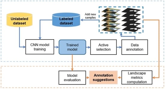
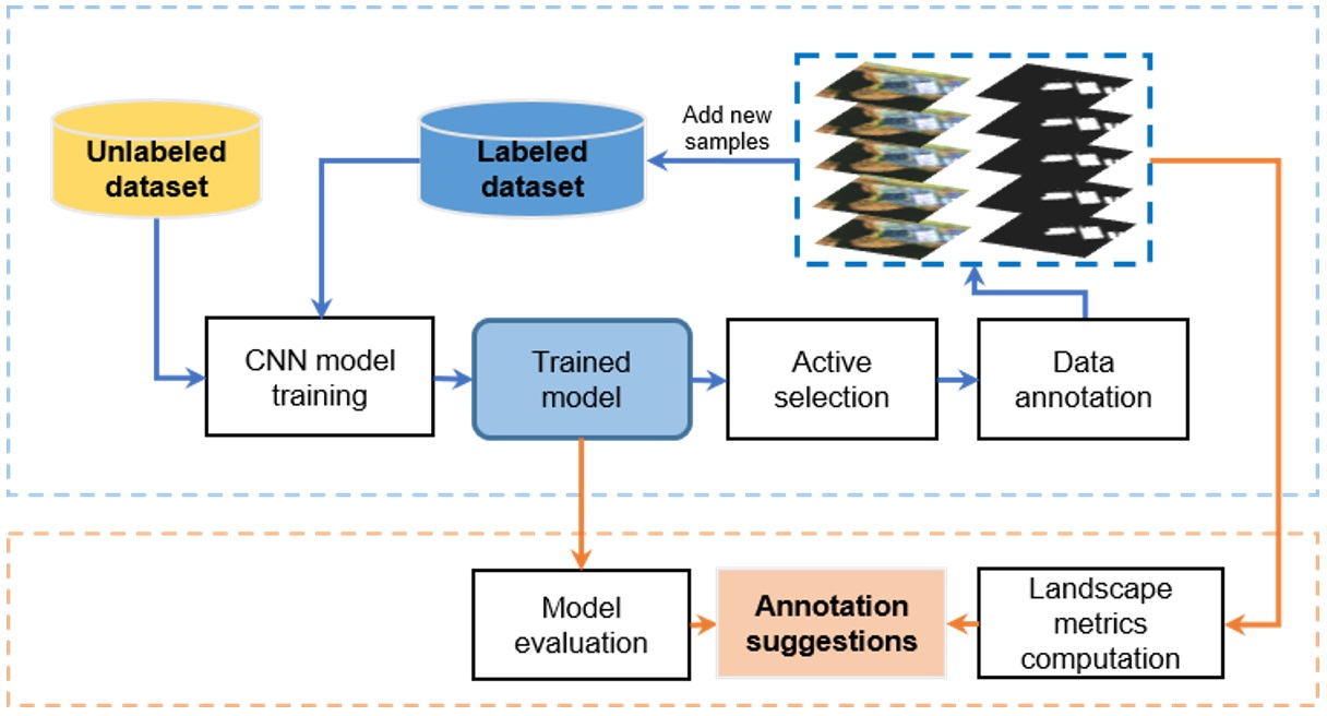
The framework for suggesting the data annotation in CNN-based building footprint mapping is shown in Figure 1, which consists of two parts: deep active learning (Figure 1a) and landscape characterization (Figure 1b). Moreover, the image tiles of a dataset should be randomly divided into two sets: a seed set, a training set, and a validation set.
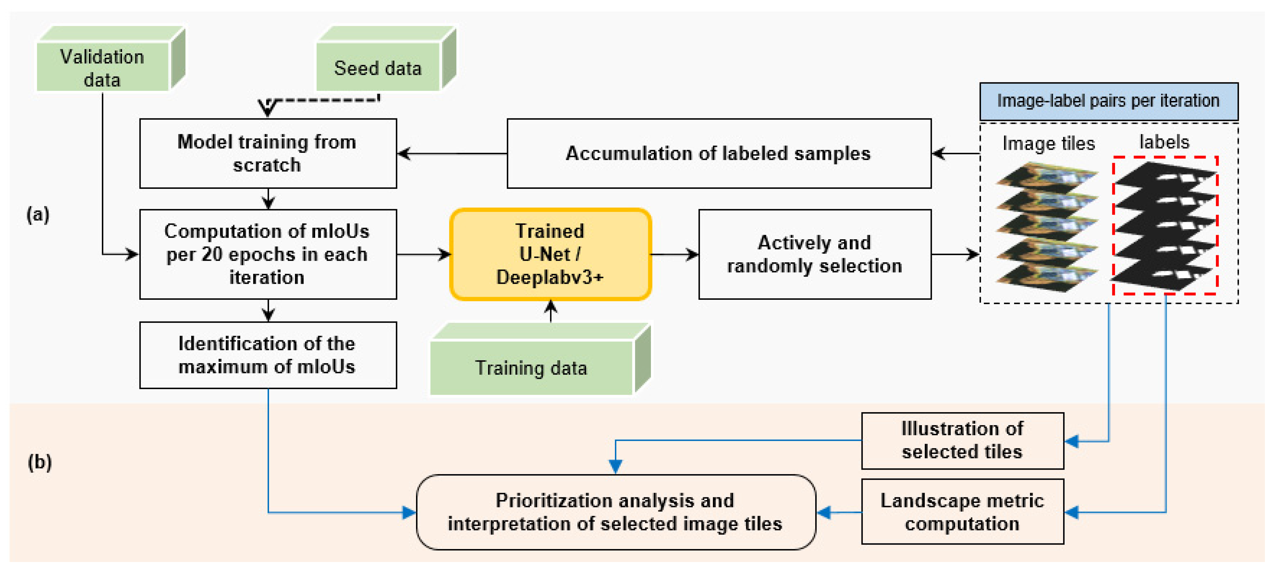
In the process of deep active learning (Figure 1a), the CNN model training is from scratch. In the first iteration, model training is based on the seed set and evaluated based on the validation set. Starting with the second iteration, all image tiles in the training set are predicted using the trained model obtained in the previous iteration, and the prediction result of each pixel in an image tile, (i.e., the probability value that a pixel is classified as building or non-building) is scored using active learning strategies. A score is given for the image tile by averaging the scores of pixels. The higher the score of the image tile, the more informative the image tile is. A fixed number of image tiles with a higher score are selected per iteration from the training set. Then, all selected image tiles were combined and used for the next CNN model training from scratch, and the mIoU was computed on the validation set to assess the model performance in each iteration. In this study, the experiment of deep active learning was implemented on two Nvidia Tesla V100 GPUs, with a learning rate of 0.1, and a batch size of 64. The experiment ended when all image tiles in the training set were used. In landscape characterization (Figure 1b), a series of landscape metrics are computed based on labeled tiles selected in each iteration to comprehend the compositional and configurational patterns of building footprints during the deep active learning process. Then, the visual comparison among the selected images is implemented to illustrate the typical landscapes useful for CNN-based building footprint mapping.
2.2. Dataset and Pre-Processing
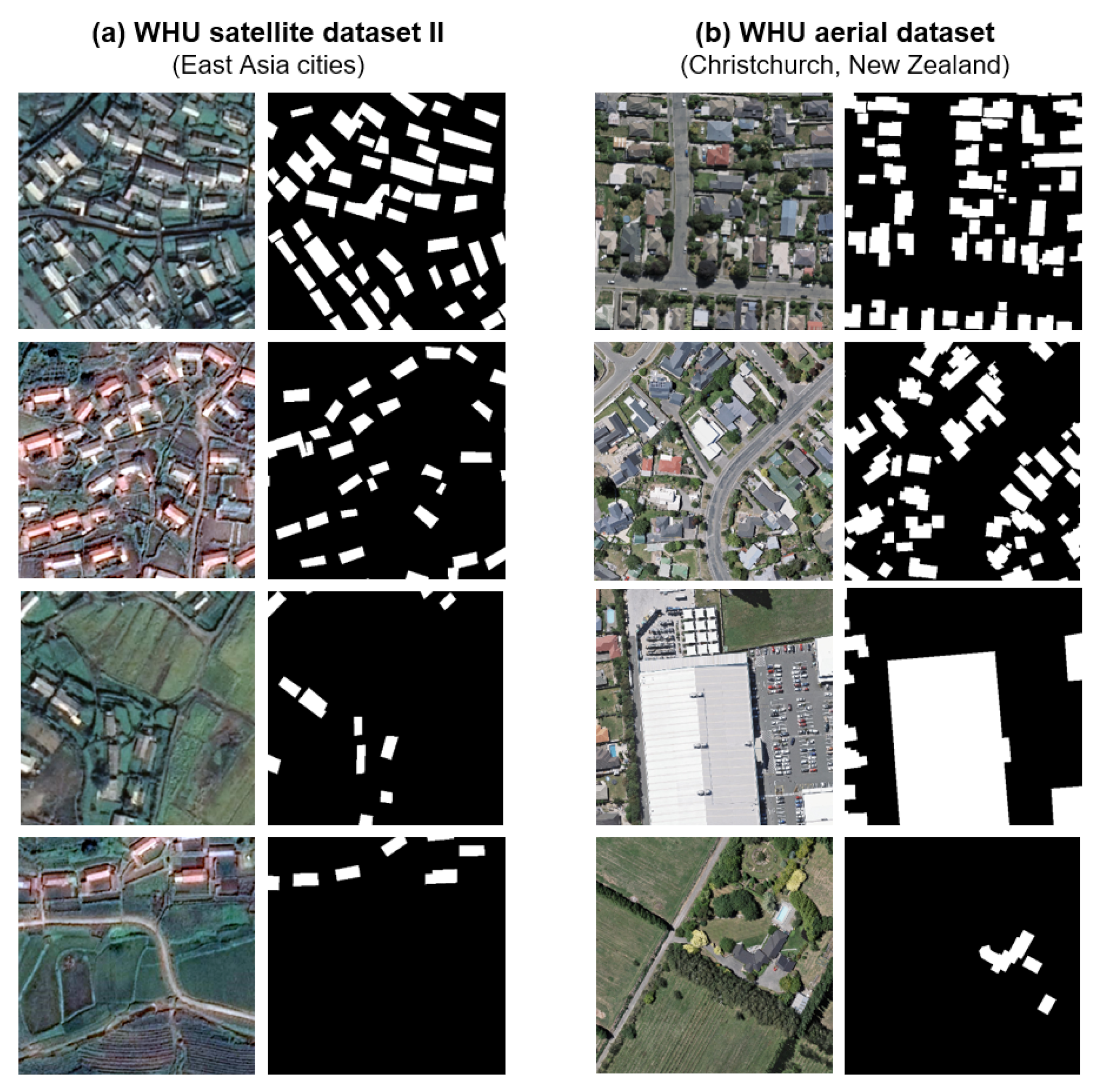
This study utilized two publicly available datasets, the WHU satellite dataset II and WHU aerial dataset. WHU satellite dataset II contains image tiles with different image colors and data sources, various densities, areas, roof colors, shapes of buildings, and similar building styles in East Asia cities (Figure 2a). It consists of 4038 image–label pairs, all of which are identical in size, (i.e., 512 × 512 pixels) and spatial resolution, (i.e., 0.45 m per pixel) [15,38]. All buildings in this dataset were completely manually identified using ArcGIS software. We combined all image–label pairs and divided them into seed set, (i.e., 160 tiles), training set, (i.e., 2868 tiles), and validation set, (i.e., 1010 tiles). Moreover, 160 tiles were selected in each iteration (Table 2). Moreover, WHU aerial dataset contains the image tiles with buildings of different densities, sizes, and shapes in Christchurch, New Zealand (Figure 2b). All buildings were generated by manually editing the building vector data. It consists of 8189 image–label pairs with identical size, (i.e., 512 × 512 pixels) and spatial resolution, (i.e., 0.30 m) [15,38]. We divided all image–label pairs into seed set, (i.e., 320 tiles), training set, (i.e., 5822 tiles), and validation set, (i.e., 2047 tiles). A total of 320 tiles were selected in each iteration (Table 2).
2.3. U-Net and DeeplabV3+ Architectures
This study used two SOTA CNN architectures in building extractions, U-Net and DeeplabV3+, in the proposed framework (Figure 1).
U-Net has symmetric structures including encoder, decoder, and skip-connection. Encoder and decoder have the same number of convolutional blocks, and blocks in the same level of encoder and decoder are connected by skip-connection. Max pooling layers reduce the dimension in the encoder and upsample layers increase the dimension in the decoder [39,40]. In our work, the upsample layers are implemented by bilinear interpolation. Convolutional blocks in different layers extract multi-scale information, and skip-connection transfers multi-scale information from the encoder’s block to the decoder’s block at the same level. The structure of the U-Net used in this study is presented in Figure 3.
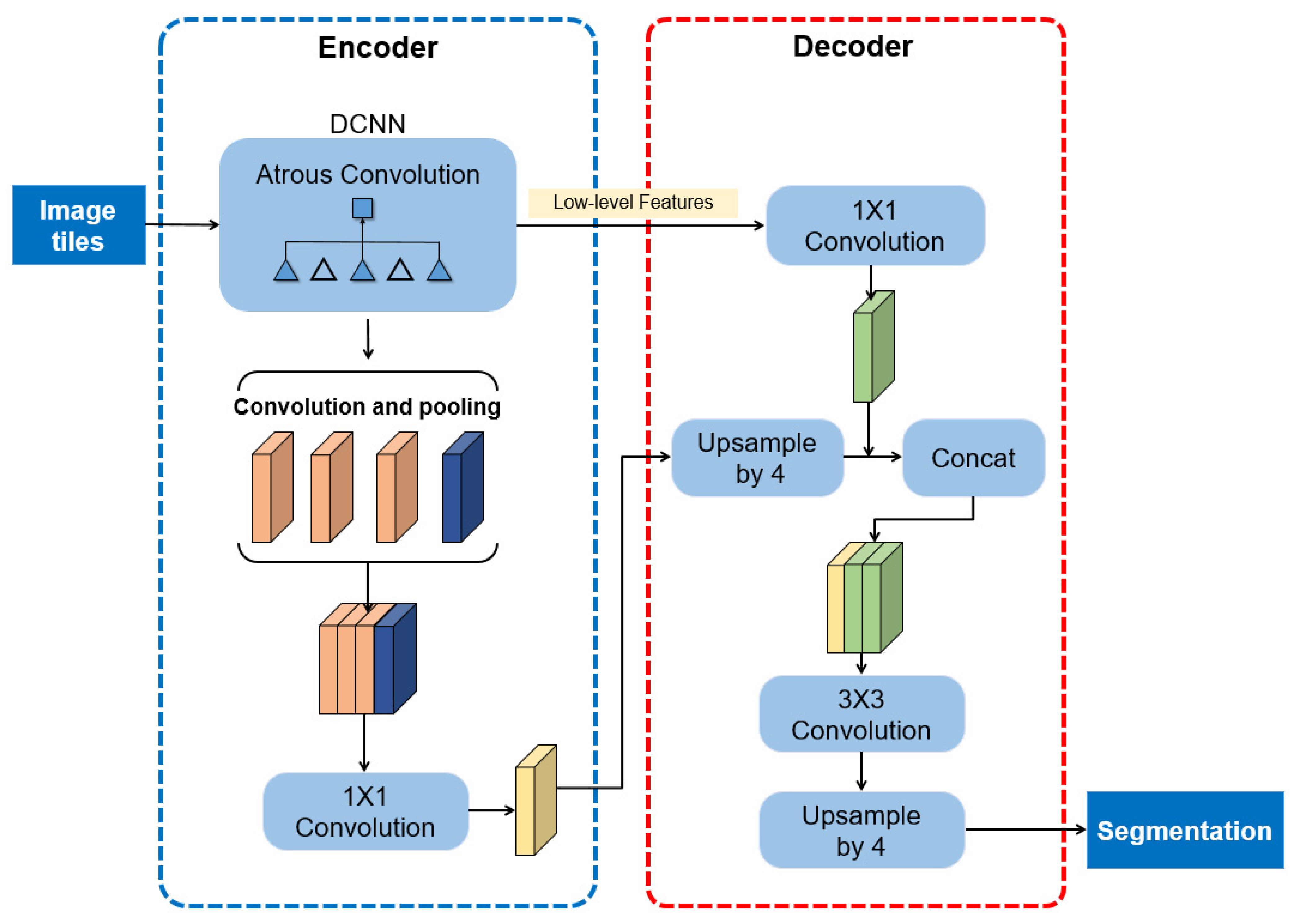
DeepLabV3+ is one of the top-performing networks in semantic segmentation that is an extension of DeeplabV3 by using an encoder and decoder structure to improve the segmentation results [41]. It encodes multi-view information by DeepLabV3 and uses the corresponding low-level features in the decoder (Figure 4). In this study, a lightweight Deep Convolutional Neural Networks (DCNNs), namely MobileNetV2, was used as the backbone of DeepLabV3. Residual blocks are also used in MobileNetV2. In DCNNS, subsampling such as pooling and convolution is used to enlarge the receptive field and reduce the computation. Atrous convolution and ASPP segment the image precisely by extracting multi-scale information at different dilation rates. In DeepLabV3+, atrous convolution is improved as atrous separable convolution, which combines atrous convolution and depthwise separable convolution to significantly speed up the computation. For ASPP, the parallel modules were used to improve the performance. In the decoder, the features are bilinearly upsampled using a factor of four and concatenated with the low-level features derived from DCNNs. Then, several 3 × 3 convolutions are used to refine the features followed by another simple bilinear upsampling using a factor of four.
2.4. Active Learning and Random Selection
By incorporating the CNN model, three active learning strategies were used to iteratively select the informative image tiles, including margin sampling, entropy, and vote entropy. Additionally, random sampling was used as a baseline method for evaluating the performance of active learning strategies that were not dependent on the CNN model. Margin sampling is an uncertainty-based technique that calculates the difference between an image tile’s first and second-largest probability and selects the samples with the smallest difference [42]. Entropy is another method based on the uncertainty that ranks all unlabeled image tiles in descending order by computing Shannon’s entropy and selecting the tiles with high entropy [42]. Vote entropy with Monte-Carlo (MC) Dropout is a query-by-committee strategy that quantifies committee disagreement and favors samples with the highest entropy [42].
where and denote the labels with the first and second-largest probabilities, respectively.
where ranges over all possible labels of .
denotes the number of votes received by a label from a committee member and C denotes the total number of committee members.
2.5. Landscape Metrics
Using the open-source Python landscape characterization library, a series of landscape metrics was computed to better comprehend the landscape characteristics of selected tiles in each iteration [43]. Since the images and labels in this study have a uniform size, (i.e., 512 × 512 pixels), and the class-level landscape metrics measure the spatial pattern of the focal class in a landscape [44], we treated each label as a landscape (Figure 1), considered the building footprint as the focal class in the landscape, and calculated the percentage (PERCENT), number of patches (NP), edge density (ED), and landscape shape index (LSI) for building class. The four landscape metrics present the area, number, edge complexity, and aggregation of buildings in the landscape, which are easily understood and visually identified by data annotators. Then, in each iteration, we determined the average condition of morphological features of the building class by computing these metrics for every selected landscape, (i.e., label) and calculating the average of all values.
Based on the equation and description of landscape metrics proposed by McGarigal et al. (2012) [34,43], we presented the four metrics used in this study as follows:
The class-level PERCENT of building class in a landscape is calculated as follows:
where A is the area of the landscape, is the area of the patch i of building. PERCENT ranges between 0 and 100. PERCENT approaches 0 as building pixels become rare in the landscape and approaches 100 as the entire landscape is covered by building pixels.
The class-level NP of building class in a landscape is computed as follows:
where represents the total number of building patches in the landscape. NP has a greater than 0, and there is no upper limit.
The class-level ED of building class in a landscape is computed as follows:
where A is the area of the landscape, represents the length of the edge between building and non-building. ED is equal to and greater than 0, without limitation. ED is equal to 0 when all pixels are building or non-building class.
The class-level LSI of building class in a landscape is computed as follows:
where A denotes the area of the landscape, represents the total edge between class i and other classes adjacent to the building class. LSI values are greater and equal to 1, without limit. LSI value is equal to 1 when the landscape consists of a signal building patch. LSI value increases without limit when the building patches become more and more disaggregated.
2.6. Selection of Best Model per Iteration
To select the best model per iteration and understand the change in model performance according to the increase in the number of input tiles, we evaluated the model performance per iteration using the mean intersection over union (mIoU) [45]. For each class, the intersection over union (IoU) refers to the ratio of intersection and union of prediction and ground truth. The mIoU is the mean of IoU values of all classes, which was computed as follows:
where k + 1 is the total number of classes. and are the pixels’ number in true pixel class i that are predicted to be in i and j, respectively. is the number of pixels belonging to j that are predicted to be class i.
Based on the confusion matrix between prediction and ground truth, the mIoU could be simplified as follows:
where k + 1 is the total number of classes. TP, FN, and FP represent the true positives, false negatives, and false positives, respectively.
In this study, there are 100 epochs per iteration. We saved one trained model every 20 epochs (Figure 1) and evaluated the model performance by segmenting the image tiles of the validation set using the saved model and computing mIoU between predicted tiles and labels. The maximum of the five mIoU values was used to indicate the model performance in each iteration. The mIoU values vary from 0 and 1, and the greater the mIoU value, the better the model performance.
3. Results
3.1. Comparison of Active Learning Strategies and Baseline Model
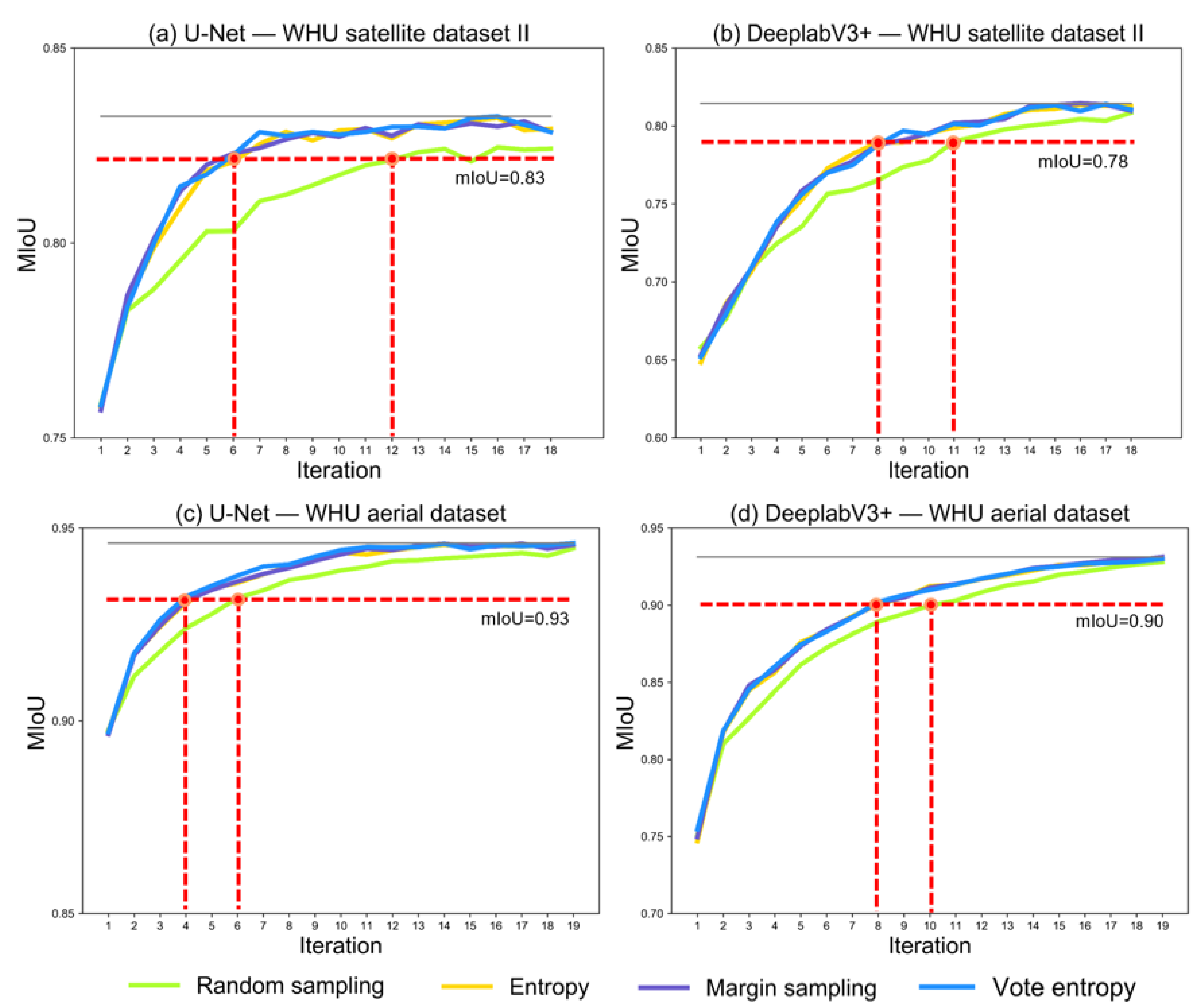
Figure 5 presents the model performance quantified by mIoU in the iterations of the deep active learning loop. The mIoU values based on WHU satellite dataset II are presented in Figure 5a,b, and the mIoU values based on WHU aerial dataset are presented in Figure 5c,d.
The mIoU value in the first iteration of each subgraph represents the performance of the model trained based on the seed set. Based on WHU satellite dataset II (Figure 5a,b), both models performed not badly, with a mIoU of 0.75 for U-Net and 0.65 for DeeplabV3+. Similarly, based on WHU aerial dataset (Figure 5c,d), the mIoU values of the two models are 0.89 and 0.75, respectively. In terms of mIoU values, CNN trained on the seed sets provide a good initial learner for deep active learning in the next iteration.
From the second iteration, the consistent results could be observed for U-Net and DeeplabV3+ based on the two datasets (Figure 5): (1) the mIoU value increases with the increase in the number of labeled tiles selected via active learning and random sampling; (2) before the last iteration, models with the three active learning strategies surpassed those with random sampling; (3) it is impossible to determine which active learning strategy is better for both two models; (4) in the last iteration, all image–label pairs were used, and models with active learning strategies had the equivalent performance with those with random sampling.
Although the U-Net and DeeplabV3+ learned more information while the number of input image–label pairs increased; however, compared to random sampling, the three active learning strategies allow the two CNN models to learn more useful information during the process. Specifically, compared to random sampling, active learning reduced the number of image tiles to be annotated while achieving the same model performance (Figure 5 and Table 3). For example, based on WHU satellite dataset II, U-Net with active learning in the sixth iteration has the equivalent performance, (i.e., mIoU of 0.83) to that in the twelfth iteration (Figure 5a), and 960 tiles do not need to be annotated (Table 3); DeeplabV3+ with active learning in the eighth iteration has the equivalent performance, (i.e., mIoU of 0.80) to that in the eleventh iteration (Figure 5b), and 480 tiles do not need to be annotated (Table 3). Moreover, based on WHU aerial dataset, U-Net with active learning in the fourth iteration has the equivalent performance, (i.e., mIoU of 0.93) to that in the sixth iteration (Figure 5c), and 640 tiles do not need to be annotated (Table 3); DeeplabV3+ with active learning in the eighth iteration has the equivalent performance, (i.e., mIoU of 0.90) to that in the tenth iteration (Figure 5d), and 640 tiles do not need to be annotated (Table 3).
3.2. Landscape Features of Selected Image Tiles Based on U-Net and DeeplabV3+
The CNN models were trained on the seed set in the first iteration, and the selection of image tiles via active learning and random sampling started from the second iteration.
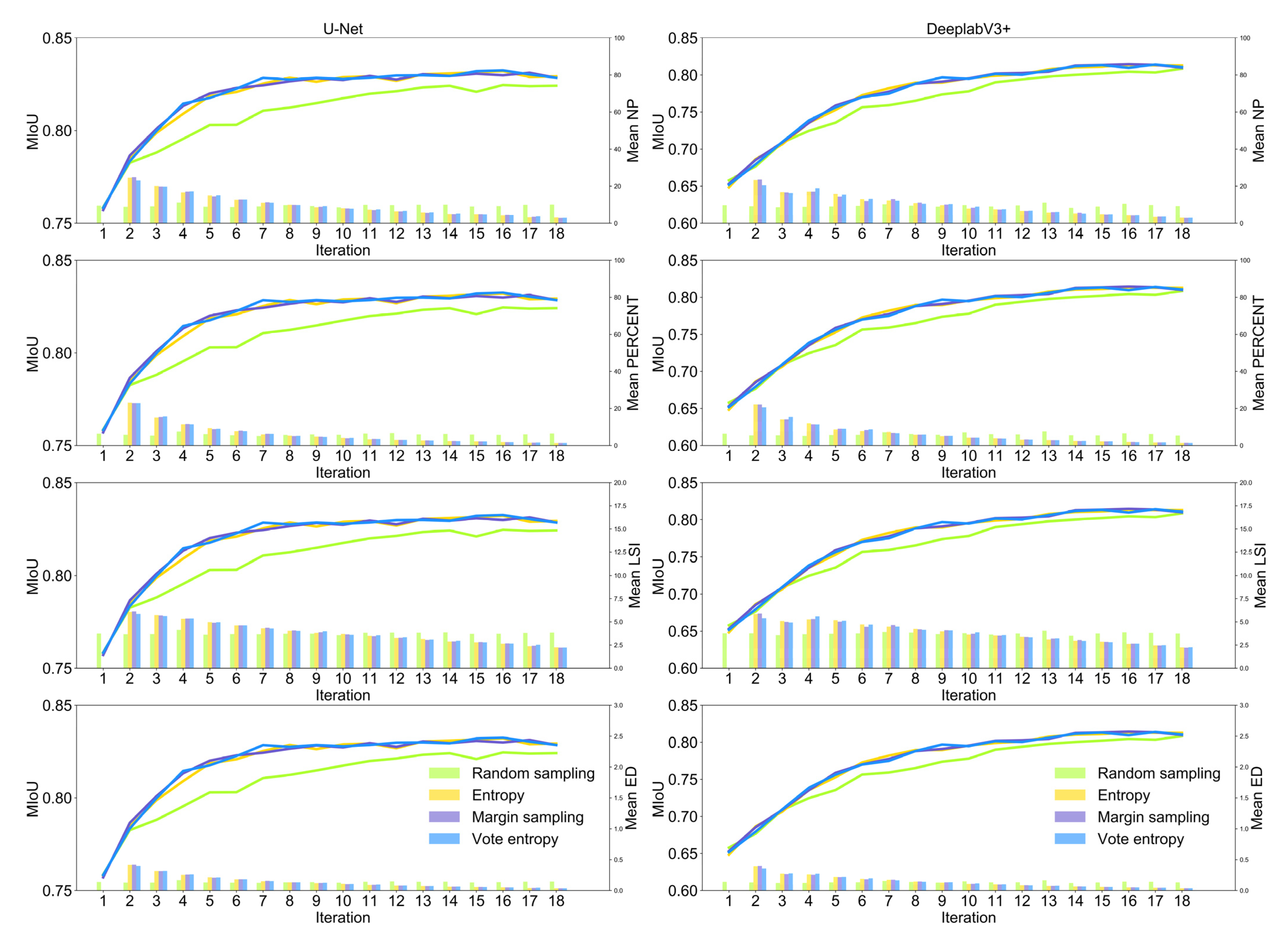
Figure 6 presents the landscape patterns of tiles selected actively and randomly in each iteration from WHU satellite dataset II. For the tiles selected via active learning strategies, mean NP, mean PERCENT, mean LSI, and mean ED have been moving downward with the increasing number of tiles for both U-Net and DeeplabV3+ from the second iteration to the last iteration. However, the values of landscape metrics remained largely stable throughout the sample selection process for random sampling. This reveals that the image tiles with more building patches, larger areas of buildings, longer edges of buildings, and more dispersed building distribution patterns are more effective for both U-Net and DeeplabV3+ in building footprint mapping.
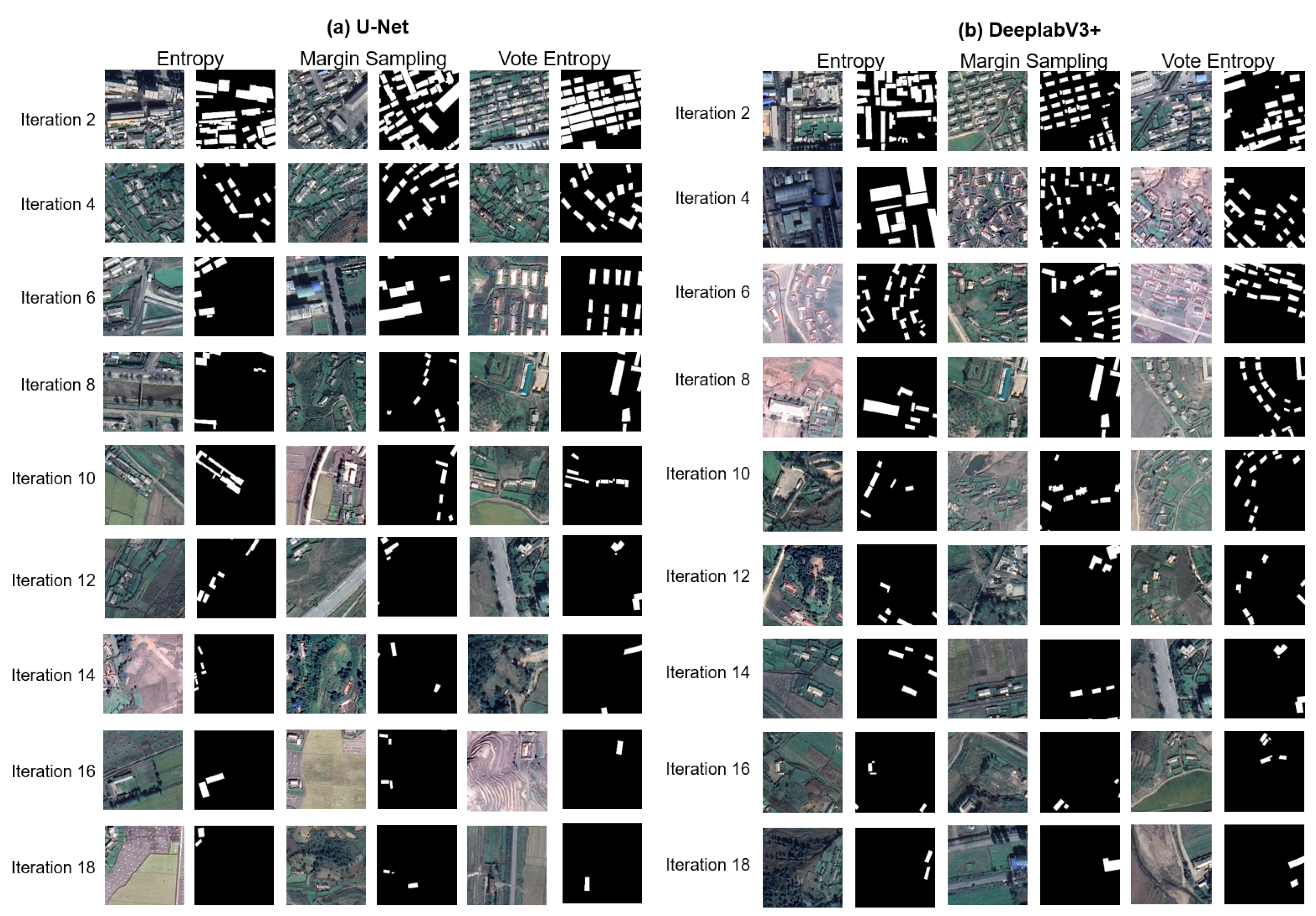
Figure 7 presents typical examples of the selected image–label pairs from WHU satellite dataset II in different iterations, which could provide us with a more figurative picture of the priority in data selection via active learning. The first iteration was to build the initial learner by training models on the seed set. Thus, among the 18 iterations in the experiment based on WHU satellite dataset II, we display the image–label pairs from the second iteration. To present the difference in landscape patterns more clearly, only the examples in even-numbered iterations are presented. Clearly, image tiles with more building patches, larger areas of buildings, longer edges of buildings, and more dispersed building distribution patterns appeared in the first few iterations. As the number of iterations increases, image tiles have fewer building patches.
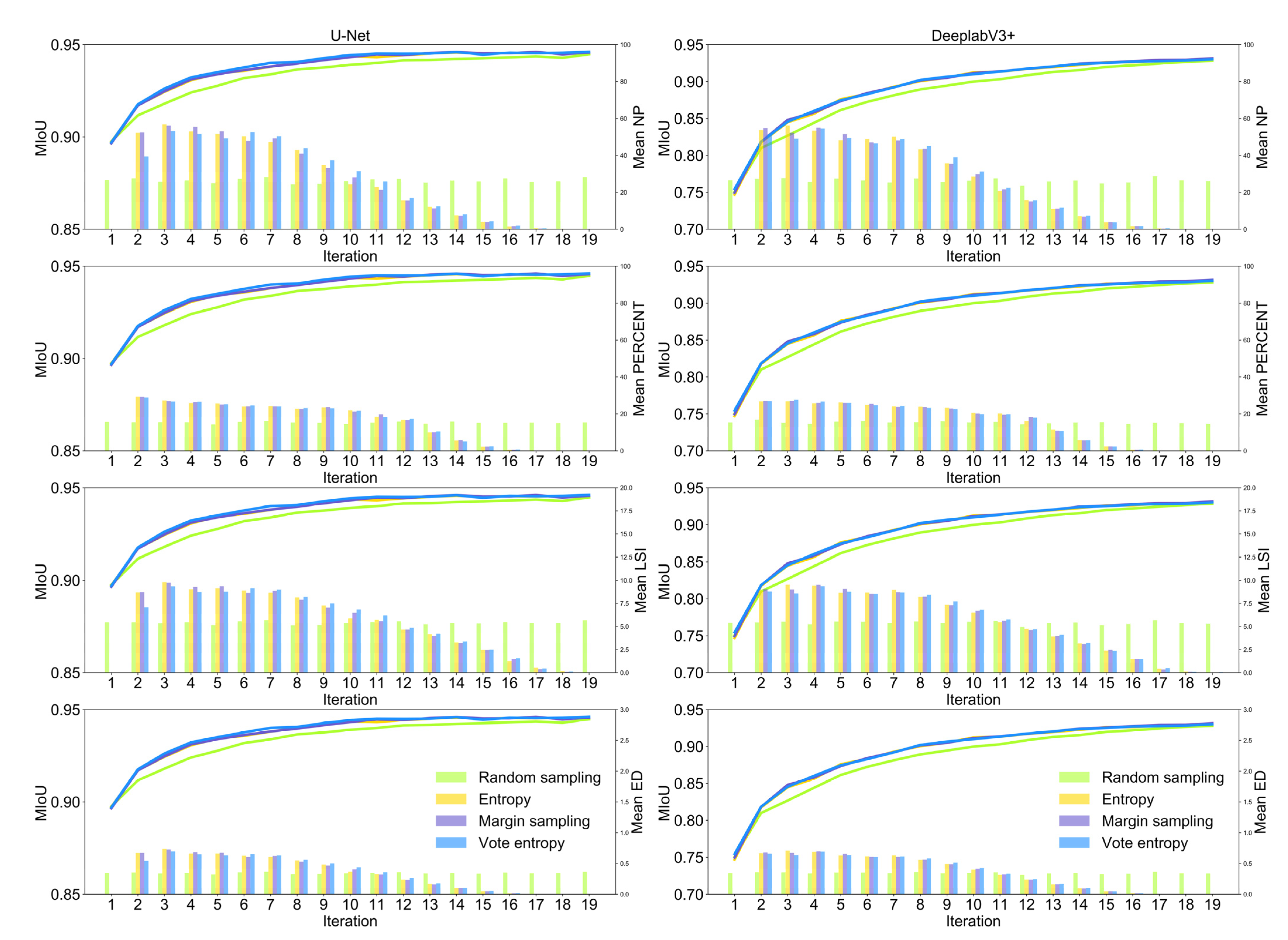
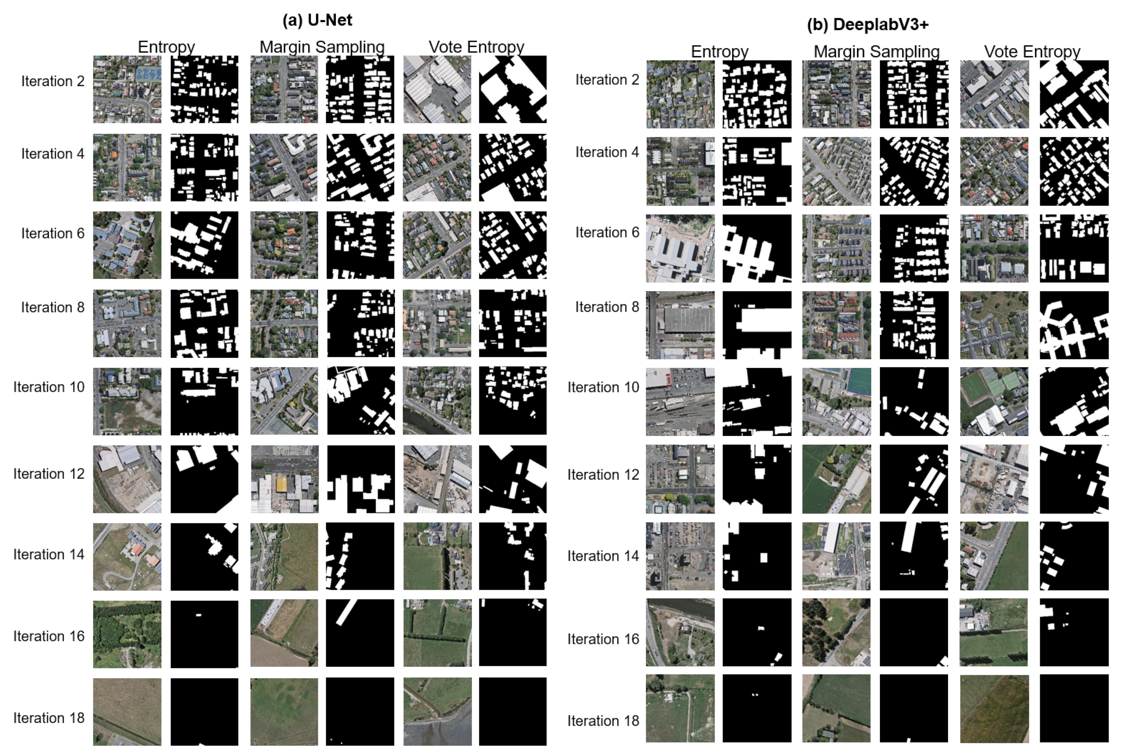
We observed similar results based on the experiment based on WHU aerial dataset. The mean NP, mean PERCENT, mean LSI, and mean ED decreased with the increasing number of tiles for both U-Net and DeeplabV3+ from the second iteration to the last iteration, and the values of landscape metrics computed based on randomly selected image tiles are relatively stable throughout the deep active learning loop (Figure 8). Among the 19 iterations in the experiment based on WHU aerial dataset, we show the actively selected image–label pairs in even-numbered iterations from the second iterations (Figure 9), and similar changes in landscape patterns were observed. It should be noted that WHU aerial dataset includes many image tiles without buildings, which often appeared in the last few iterations, (e.g., 18th and 19th iterations), resulting in the low values of landscape metrics (Figure 8 and Figure 9).
4. Discussion
This study proposed an easily interpretable framework incorporating a deep active learning loop and landscape characterization that could be used for reducing the number of unlabeled images to be annotated and understanding what kind of labeled image tiles are advantageous for CNN-based building footprint mapping in real-world applications. In this study, two SOTA CNN architectures, DeeplabV3+ with MobileNet backbone and U-Net, were used. Each of them was integrated with three active learning strategies to create its own deep active learning process. In terms of landscape characterization, four class-level landscape metrics related to the number, area, edge, and aggregation of building patches were considered; these metrics provide a more graphic interpretation for “informative” image tiles chosen by deep active learning that might benefit the manual data annotation in practice.
Based on the experiments on WHU satellite dataset II and WHU aerial dataset, we found the tiles with greater values in PERCENT, NP, ED, and LSI were selected with preference by both U-Net and DeeplabV3+ (Figure 6 and Figure 8). In other words, when selecting image tiles for data annotation based on visual interpretation, special consideration should be given to image tiles with more buildings, larger areas of buildings, longer edges between buildings and other landscape factors, and more dispersed spatial distribution of buildings (Figure 7 and Figure 9). These tiles might contain more information on the contact between a building and other landscape factors, such as a building and vegetation or a building and a road, enabling the model to learn the various information about buildings and other landscape factors more quickly.
It should be noted that there are many types of landscape metrics, (e.g., area, edge, shape, core area, contrast, and aggregation) and three levels for landscape metric computation, (i.e., patch, class, and landscape levels) [34,46,47]. In our study, we subjectively selected four class-level metrics characterizing the area, number, edge, and aggregation of building patches that are easily interpretable for data labelers. Moreover, several of the metrics are correlated with each other. Dimensionality reduction techniques, such as principal component analysis (PCA), cluster analysis, and the correlation test, should be used to examine the correlation between certain metrics while many metrics are used together [37,48,49].
The two representative benchmark building datasets used in this study could explain to some extent the feasibility of the proposed framework and suggestions for data annotation in CNN-based building footprint mapping. First, WHU satellite dataset II derived from different data sources covers several cities and diverse landscapes in a large geographic region in East Asia, (i.e., 860 km2), which is often used to assess the generalization ability of newly proposed models in practical applications, especially large-scale building footprint mapping [15,50]. WHU aerial dataset cover 450 km2 in Christchurch, the second-largest city in New Zealand [15], consisting of different urban LULC types, (e.g., urban and suburban areas, residential areas, industrial areas, and commercial areas), which is an ideal dataset to assess the robustness of newly proposed models [50]. Second, the two building datasets have the close spatial resolution, (i.e., 0.45 m and 0.3 m), and the same size of tiles, (i.e., 512 × 512 pixels) (Table 1), and the similar data splitting was used for the two experiments, (i.e., 4% of tiles for the seed set, 4% of titles for the selection per iteration from the training set, and 25% of titles for the validation set) (Table 2). These facts allow the results of experiments to be compared and summarized. Thirdly, sufficient image tiles in the training set, (i.e., 2868 tiles for WHU satellite dataset II and 5822 tiles for WHU aerial dataset) ensure many iterations, (i.e., 18 iterations and 19 iterations for the two experiments, respectively), (Table 2). The dynamics in model performance are fully represented in the process of deep active learning, (i.e., the increase in model performance becomes progressively slower during the deep active learning loop) (Figure 5).
However, future building footprint mapping via CNN-based VHR image segmentation should apply the results and interpretation obtained in this study with caution. The modifiable areal unit problem (MAUP), referring to how the pixel size of input data and landscape extent affect the values of landscape metrics, make the interpretation of landscape metrics quite challenging [46,49]. In our study, the results were obtained based on the datasets with close spatial resolutions, (i.e.,0.45 m and 0.30 m) and a fixed landscape extent, (i.e., 512 × 512 pixels). However, in real-world applications, despite the use of VHR satellite images, different spatial resolutions, (e.g., 0.075 m) and different sizes of input image tiles, (e.g., 128 × 128, 256 × 256, 650 × 650, 1204 × 1024) are required to handle buildings of varying scales in different study areas [51], and the obtained suggestions for data annotation might not be suitable. In addition, other open-source benchmark datasets can be used to query or confirm our proposed framework and results, especially the datasets containing different cities in different countries, such as SpaceNet 1 and 2 (Table 1).
While this study demonstrates that active learning can reduce the effort of data annotation in CNN-based building footprint mapping and that class-level landscape metrics assist in understanding the landscape characteristics of the image tiles selected during the deep active learning process, there are still some limitations. To begin with, this study examined three widely used active learning algorithms and discovered that there is no statistically significant difference between them in terms of minimizing data annotation costs and selecting landscape features. Other query tactics, such as diversity-based strategies [42] and hybrid active learning [52], could be incorporated into the proposed framework, potentially providing new insight into the models’ preference for landscape characterization. Second, while the existing procedure can assist us in determining the type of image tiles to label, the iterative framework requires additional time spent reviewing data and training models. In real-world applications, one-shot active learning may be more practical than iterative learning [53]. Thirdly, our results may enhance CNN-based building footprint mapping on VHR datasets with similar building characteristics. Experiments based on other datasets with different building styles, (e.g., residential, educational, industrial, and business), sizes, (e.g., small, medium, and large), and shapes, (e.g., round, rectangle, and irregular) should be performed to explore more general conclusion.
5. Conclusions
This study conducted preliminary tests on deep active learning and landscape characterization to quantify the performance of active learning strategies in reducing the effort of data annotation and to better understand the landscape features prioritized by deep learning models in CNN-based building footprint mapping. The study findings suggest that deep active learning can be integrated into building footprint mapping, with image tiles containing more buildings, larger building areas, and disaggregated buildings being prioritized during the deep active learning process. Our findings suggest that it is possible to reduce the efforts of data annotation in future CNN-based building footprint mapping using a simple manner, the preliminary visual screening of unlabeled image tiles based on our findings. It also inspires us to explore the landscape features preferred by models in other CNN-based thematic mappings, especially the large-scale thematic land use mapping.
Author Contributions
Z.L. led the study, collected the data, implemented data analysis, reviewed the bibliography, and wrote the paper. S.Z. participated in data processing and data analysis. J.D. participated in the study design and revised the manuscript. All authors have read and agreed to the published version of the manuscript.
Funding
This study was supported by the Strategic Priority Research Program (XDA19040301) of the Chinese Academy of Sciences (CAS), the Informatization Plan of Chinese Academy of Sciences (Grant number: CAS-WX2021PY-0109), and the Institute of Geographic Sciences and Natural Resources Research of CAS (Grant number: E0V00110YZ).
Conflicts of Interest
The authors declare no conflict of interest.
References
- Schneider, A.; Friedl, M.A.; Potere, D. A new map of global urban extent from MODIS satellite data. Environ. Res. Lett. 2009, 4, 044003. [Google Scholar] [CrossRef] [Green Version]
- Jochem, W.C.; Leasure, D.R.; Pannell, O.; Chamberlain, H.R.; Jones, P.; Tatem, A.J. Classifying settlement types from multi-scale spatial patterns of building footprints. Environ. Plan. B Urban Anal. City Sci. 2021, 48, 1161–1179. [Google Scholar] [CrossRef]
- Seto, K.C.; Sánchez-Rodríguez, R.; Fragkias, M. The New Geography of Contemporary Urbanization and the Environment. Annu. Rev. Environ. Resour. 2010, 35, 167–194. [Google Scholar] [CrossRef] [Green Version]
- Yuan, X.; Shi, J.; Gu, L. A review of deep learning methods for semantic segmentation of remote sensing imagery. Expert Syst. Appl. 2021, 169, 114417. [Google Scholar] [CrossRef]
- Zhao, F.; Zhang, C. Building Damage Evaluation from Satellite Imagery using Deep Learning. In Proceedings of the 2020 IEEE 21st International Conference on Information Reuse and Integration for Data Science (IRI), Las Vegas, NV, USA, 11–13 August 2020; pp. 82–89. [Google Scholar]
- Pan, Z.; Xu, J.; Guo, Y.; Hu, Y.; Wang, G. Deep Learning Segmentation and Classification for Urban Village Using a Worldview Satellite Image Based on U-Net. Remote Sens. 2020, 12, 1574. [Google Scholar] [CrossRef]
- Wagner, F.H.; Dalagnol, R.; Tarabalka, Y.; Segantine, T.Y.; Thomé, R.; Hirye, M. U-net-id, an instance segmentation model for building extraction from satellite images—Case study in the Joanopolis City, Brazil. Remote Sens. 2020, 12, 1544. [Google Scholar] [CrossRef]
- Rastogi, K.; Bodani, P.; Sharma, S.A. Automatic building footprint extraction from very high-resolution imagery using deep learning techniques. Geocarto Int. 2020, 37, 1501–1513. [Google Scholar] [CrossRef]
- Li, C.; Fu, L.; Zhu, Q.; Zhu, J.; Fang, Z.; Xie, Y.; Guo, Y.; Gong, Y. Attention Enhanced U-Net for Building Extraction from Farmland Based on Google and WorldView-2 Remote Sensing Images. Remote Sens. 2021, 13, 4411. [Google Scholar] [CrossRef]
- Pasquali, G.; Iannelli, G.C.; Dell’Acqua, F. Building footprint extraction from multispectral, spaceborne earth observation datasets using a structurally optimized U-Net convolutional neural network. Remote Sens. 2019, 11, 2803. [Google Scholar] [CrossRef] [Green Version]
- Touzani, S.; Granderson, J. Open Data and Deep Semantic Segmentation for Automated Extraction of Building Footprints. Remote Sens. 2021, 13, 2578. [Google Scholar] [CrossRef]
- Yang, N.; Tang, H. GeoBoost: An Incremental Deep Learning Approach toward Global Mapping of Buildings from VHR Remote Sensing Images. Remote Sens. 2020, 12, 1794. [Google Scholar] [CrossRef]
- Zhou, D.; Wang, G.; He, G.; Yin, R.; Long, T.; Zhang, Z.; Chen, S.; Luo, B. A Large-Scale Mapping Scheme for Urban Building From Gaofen-2 Images Using Deep Learning and Hierarchical Approach. IEEE J. Sel. Top. Appl. Earth Obs. Remote Sens. 2021, 14, 11530–11545. [Google Scholar] [CrossRef]
- Yang, H.L.; Yuan, J.; Lunga, D.; Laverdiere, M.; Rose, A.; Bhaduri, B. Building Extraction at Scale Using Convolutional Neural Network: Mapping of the United States. IEEE J. Sel. Top. Appl. Earth Obs. Remote Sens. 2018, 11, 2600–2614. [Google Scholar] [CrossRef] [Green Version]
- Ji, S.; Wei, S.; Lu, M. Fully Convolutional Networks for Multisource Building Extraction fom an Open Aerial and Satellite Imagery Data Set. IEEE Trans. Geosci. Remote Sens. 2018, 57, 574–586. [Google Scholar] [CrossRef]
- Chen, Q.; Wang, L.; Wu, Y.; Wu, G.; Guo, Z.; Waslander, S.L. TEMPORARY REMOVAL: Aerial imagery for roof segmentation: A large-scale dataset towards automatic mapping of buildings. ISPRS J. Photogramm. Remote Sens. 2019, 147, 42–55. [Google Scholar] [CrossRef] [Green Version]
- Van Etten, A.; Lindenbaum, D.; Bacastow, T.M. Spacenet: A remote sensing dataset and challenge series. arXiv 2018, arXiv:1807.01232. [Google Scholar]
- Mace, E.; Manville, K.; Barbu-McInnis, M.; Laielli, M.; Klaric, M.K.; Dooley, S. Overhead Detection: Beyond 8-bits and RGB. arXiv 2018, arXiv:1808.02443. [Google Scholar]
- Kang, J.; Tariq, S.; Oh, H.; Woo, S.S. A Survey of Deep Learning-Based Object Detection Methods and Datasets for Overhead Imagery. IEEE Access 2022, 10, 20118–20134. [Google Scholar] [CrossRef]
- Li, W.; He, C.; Fang, J.; Zheng, J.; Fu, H.; Yu, L. Semantic Segmentation-Based Building Footprint Extraction Using Very High-Resolution Satellite Images and Multi-Source GIS Data. Remote Sens. 2019, 11, 403. [Google Scholar] [CrossRef] [Green Version]
- Maggiori, E.; Tarabalka, Y.; Charpiat, G.; Alliez, P. Can semantic labeling methods generalize to any city? the inria aerial image labeling benchmark. In Proceedings of the 2017 IEEE International Geoscience and Remote Sensing Symposium (IGARSS), Fort Worth, TX, USA, 23–28 July 2017; pp. 3226–3229. [Google Scholar]
- Mnih, V. Machine Learning for Aerial Image Labeling; University of Toronto: Toronto, ON, Canada, 2013. [Google Scholar]
- Chen, Q.; Zhang, Y.; Li, X.; Tao, P. Extracting Rectified Building Footprints from Traditional Orthophotos: A New Workflow. Sensors 2022, 22, 207. [Google Scholar] [CrossRef]
- Rahman, A.K.M.M.; Zaber, M.; Cheng, Q.; Nayem, A.B.S.; Sarker, A.; Paul, O.; Shibasaki, R. Applying State-of-the-Art Deep-Learning Methods to Classify Urban Cities of the Developing World. Sensors 2021, 21, 7469. [Google Scholar] [CrossRef] [PubMed]
- Gergelova, M.B.; Labant, S.; Kuzevic, S.; Kuzevicova, Z.; Pavolova, H. Identification of Roof Surfaces from LiDAR Cloud Points by GIS Tools: A Case Study of Lučenec, Slovakia. Sustainability 2020, 12, 6847. [Google Scholar] [CrossRef]
- Li, J.; Meng, L.; Yang, B.; Tao, C.; Li, L.; Zhang, W. LabelRS: An Automated Toolbox to Make Deep Learning Samples from Remote Sensing Images. Remote Sens. 2021, 13, 2064. [Google Scholar] [CrossRef]
- Xia, G.-S.; Wang, Z.; Xiong, C.; Zhang, L. Accurate Annotation of Remote Sensing Images via Active Spectral Clustering with Little Expert Knowledge. Remote Sens. 2015, 7, 15014–15045. [Google Scholar] [CrossRef] [Green Version]
- Ren, P.; Xiao, Y.; Chang, X.; Huang, P.-Y.; Li, Z.; Gupta, B.B.; Chen, X.; Wang, X. A survey of deep active learning. ACM Comput. Surv. (CSUR) 2021, 54, 1–40. [Google Scholar] [CrossRef]
- Robinson, C.; Ortiz, A.; Malkin, K.; Elias, B.; Peng, A.; Morris, D.; Dilkina, B.; Jojic, N. Human-machine collaboration for fast land cover mapping. In Proceedings of the AAAI Conference on Artificial Intelligence, New York, NY, USA, 7–12 February 2020; pp. 2509–2517. [Google Scholar]
- Hamrouni, Y.; Paillassa, E.; Chéret, V.; Monteil, C.; Sheeren, D. From local to global: A transfer learning-based approach for mapping poplar plantations at national scale using Sentinel-2. ISPRS J. Photogramm. Remote Sens. 2021, 171, 76–100. [Google Scholar] [CrossRef]
- Bi, H.; Xu, F.; Wei, Z.; Xue, Y.; Xu, Z. An active deep learning approach for minimally supervised PolSAR image classification. IEEE Trans. Geosci. Remote Sens. 2019, 57, 9378–9395. [Google Scholar] [CrossRef]
- Xu, G.; Zhu, X.; Tapper, N. Using convolutional neural networks incorporating hierarchical active learning for target-searching in large-scale remote sensing images. Int. J. Remote Sens. 2020, 41, 4057–4079. [Google Scholar] [CrossRef]
- Yang, L.; Zhang, Y.; Chen, J.; Zhang, S.; Chen, D.Z. Suggestive annotation: A deep active learning framework for biomedical image segmentation. In Proceedings of the International Conference on Medical Image Computing and Computer-Assisted Intervention, Quebec City, QC, Canada, 11–13 September 2017; pp. 399–407. [Google Scholar]
- McGarigal, K.; Cushman, S.A.; Ene, E. FRAGSTATS v4: Spatial Pattern Analysis Program for Categorical and Continuous Maps. Computer Software Program Produced by the Authors at the University of Massachusetts, Amherst. 2012, Volume 15. Available online: http://www.umass.edu/landeco/research/fragstats/fragstats.html (accessed on 1 May 2022).
- Frazier, A.E.; Kedron, P. Landscape metrics: Past progress and future directions. Curr. Landsc. Ecol. Rep. 2017, 2, 63–72. [Google Scholar] [CrossRef] [Green Version]
- Li, Z.; Roux, E.; Dessay, N.; Girod, R.; Stefani, A.; Nacher, M.; Moiret, A.; Seyler, F. Mapping a knowledge-based malaria hazard index related to landscape using remote sensing: Application to the cross-border area between French Guiana and Brazil. Remote Sens. 2016, 8, 319. [Google Scholar] [CrossRef] [Green Version]
- Li, Z.; Feng, Y.; Dessay, N.; Delaitre, E.; Gurgel, H.; Gong, P. Continuous monitoring of the spatio-temporal patterns of surface water in response to land use and land cover types in a Mediterranean lagoon complex. Remote Sens. 2019, 11, 1425. [Google Scholar] [CrossRef] [Green Version]
- Yang, H.; Xu, M.; Chen, Y.; Wu, W.; Dong, W. A Postprocessing Method Based on Regions and Boundaries Using Convolutional Neural Networks and a New Dataset for Building Extraction. Remote Sens. 2022, 14, 647. [Google Scholar] [CrossRef]
- Ronneberger, O.; Fischer, P.; Brox, T. U-net: Convolutional networks for biomedical image segmentation. In Proceedings of the International Conference on Medical Image Computing and Computer-Assisted Intervention, Munich, Germany, 5–9 October 2015; pp. 234–241. [Google Scholar]
- Siddique, N.; Paheding, S.; Elkin, C.P.; Devabhaktuni, V. U-Net and Its Variants for Medical Image Segmentation: A Review of Theory and Applications. IEEE Access 2021, 9, 82031–82057. [Google Scholar] [CrossRef]
- Chen, L.-C.; Zhu, Y.; Papandreou, G.; Schroff, F.; Adam, H. Encoder-decoder with atrous separable convolution for semantic image segmentation. In Proceedings of the European Conference on Computer Vision (ECCV), Munich, Germany, 8–14 September 2018; pp. 801–818. [Google Scholar]
- Settles, B. Active Learning Literature Survey; University of Wisconsin-Madison: Madison, WI, USA, 2009. [Google Scholar]
- Bosch, M. PyLandStats: An open-source Pythonic library to compute landscape metrics. PLoS ONE 2019, 14, e0225734. [Google Scholar] [CrossRef] [PubMed] [Green Version]
- Wang, X.; Blanchet, F.G.; Koper, N. Measuring habitat fragmentation: An evaluation of landscape pattern metrics. Methods Ecol. Evol. 2014, 5, 634–646. [Google Scholar] [CrossRef]
- Long, J.; Shelhamer, E.; Darrell, T. Fully convolutional networks for semantic segmentation. In Proceedings of the IEEE Conference on Computer Vision and Pattern Recognition, Boston, MA, USA, 7–12 June 2015; pp. 3431–3440. [Google Scholar]
- Uuemaa, E.; Antrop, M.; Roosaare, J.; Marja, R.; Mander, Ü. Landscape Metrics and Indices: An Overview of Their Use in Landscape Research. Living Rev. Landsc. Res. 2009, 3, 1–28. [Google Scholar] [CrossRef]
- Plexida, S.G.; Sfougaris, A.I.; Ispikoudis, I.P.; Papanastasis, V.P. Selecting landscape metrics as indicators of spatial heterogeneity—A comparison among Greek landscapes. Int. J. Appl. Earth Obs. Geoinf. 2014, 26, 26–35. [Google Scholar] [CrossRef]
- Cushman, S.A.; McGarigal, K.; Neel, M.C. Parsimony in landscape metrics: Strength, universality, and consistency. Ecol. Indic. 2008, 8, 691–703. [Google Scholar] [CrossRef]
- Openshaw, S. The modifiable areal unit problem. Quant. Geogr. A Br. View 1981, 60–69. Available online: https://cir.nii.ac.jp/crid/1572824498971908736 (accessed on 1 May 2022).
- Chen, F.; Wang, N.; Yu, B.; Wang, L. Res2-Unet, a New Deep Architecture for Building Detection from High Spatial Resolution Images. IEEE J. Sel. Top. Appl. Earth Obs. Remote Sens. 2022, 15, 1494–1501. [Google Scholar] [CrossRef]
- Zhao, K.; Kang, J.; Jung, J.; Sohn, G. Building Extraction from Satellite Images Using Mask R-CNN with Building Boundary Regularization. In Proceedings of the 2018 IEEE/CVF Conference on Computer Vision and Pattern Recognition Workshops (CVPRW), Salt Lake City, UT, USA, 18–22 June 2018; pp. 242–2424. [Google Scholar]
- Wu, X.; Chen, C.; Zhong, M.; Wang, J. HAL: Hybrid active learning for efficient labeling in medical domain. Neurocomputing 2021, 456, 563–572. [Google Scholar] [CrossRef]
- Jin, Q.; Yuan, M.; Qiao, Q.; Song, Z. One-shot active learning for image segmentation via contrastive learning and diversity-based sampling. Knowl. Based Syst. 2022, 241, 108278. [Google Scholar] [CrossRef]
Figure 1.
The framework for suggestive data annotation in CNN-based building footprint mapping. Part (a) represents the process of deep active learning for building footprint mapping. Part (b) represents the steps of interpreting selected image tiles in each iteration by landscape characterization and visual comparison. The dotted arrow denotes the model training in the first iteration based on the seed set. The black arrows denote the steps in the deep active learning process. The blue arrows denote the steps in the interpretation of selected building/non-building landscapes.

Figure 2.
Illustration of image–label pairs in WHU satellite dataset II covering East Asia cities (a) and WHU aerial dataset covering Christchurch, New Zealand (b). For each dataset, the first column presents the RGB image with 512 × 512 pixels, and the second column presents the labels with white building pixels.

Figure 3.
The U-Net architecture used in this study.

Figure 4.
The DeepLabV3+ architecture used in this study.

Figure 5.
Comparison of active learning and random sampling based on WHU satellite dataset II and WHU aerial dataset. (a,b) Represent the results based on WHU satellite dataset II for U-Net and DeeplabV3+, respectively. (c,d) Represent the results based on WHU aerial dataset for U-Net and DeeplabV3+, respectively. The x-axis and y-axis represent the number of iterations and mIoU values in each iteration, respectively. The horizontal red dotted lines indicate one mIoU for comparing the models with active learning and models with random sampling, and the vertical red dotted lines indicate the number of iterations when the model performance is archived.

Figure 6.
Landscape patterns of selected tiles in each iteration via three active learning strategies and random sampling from WHU satellite dataset II. The x-axis indicates the iterations of model training. The left y-axis indicates the value of mIoU in each iteration. The right y-axis indicates the value of the landscape metrics computed based on selected image tiles in each iteration.

Figure 7.
Example of image–label pairs selected by active learning strategies based on U-Net (a), DeeplabV3+ (b), and WHU satellite dataset II.
Figure 7.
Example of image–label pairs selected by active learning strategies based on U-Net (a), DeeplabV3+ (b), and WHU satellite dataset II.

Figure 8.
Landscape patterns of selected tiles in each iteration via three active learning strategies and random sampling from WHU aerial dataset. The x-axis indicates the iterations of model training. The left y-axis indicates the value of mIoU in each iteration. The right y-axis indicates the value of the landscape metrics computed based on selected image tiles in each iteration.

Figure 9.
Example of image–label pairs selected by active learning strategies based on U-Net (a), DeeplabV3+ (b), and WHU aerial dataset.
Figure 9.
Example of image–label pairs selected by active learning strategies based on U-Net (a), DeeplabV3+ (b), and WHU aerial dataset.


Table 1.
Summary of frequently used public datasets in CNN-based building footprint mapping.
| Datasets | Resolution (m) | Number of Image–Label Pairs | Size of Tiles (Pixels) | Geolocation | References |
|---|---|---|---|---|---|
| WHU satellite dataset I | 0.3 to 2.5 | 204 | 512 × 512 | 10 cities worldwide | [15] |
| WHU satellite dataset II | 0.45 | 4038 | 512 × 512 | East Asia cities | [15] |
| WHU aerial dataset | 0.3 | 8189 | 512 × 512 | Christchurch, New Zealand | [15] |
| Aerial imagery for roof segmentation | 0.075 | 1047 | 10,000 × 10,000 | Christchurch, New Zealand | [16] |
| SpaceNet 1 | 0.5 | 9735 | 439 × 407 | Rio de Janeiro, Brazil | [17,18,19] |
| SpaceNet 2 | 0.3 | 10,593 | 650 × 650 | Las Vegas, Paris, Shanghai, Khartoum | [17,19,20] |
| Inria Aerial Image Labeling Dataset | 0.3 | 360 | 5000 × 5000 | 10 cities worldwide | [21] |
| Massachusetts Buildings Dataset | 1 | 151 | 1500 × 1500 | Massachusetts, USA | [22] |
Table 2.
The seed set, training set, and validation set of building datasets used in this study.
| Dataset | Seed Set | Training Set | Validation Set | Tiles Selected per Iteration | Number of Iterations |
|---|---|---|---|---|---|
| WHU satellite dataset II | 160 tiles | 2868 tiles | 1010 tiles | 160 tiles | 18 |
| WHU aerial dataset | 320 tiles | 5822 tiles | 2047 tiles | 320 tiles | 19 |
Table 3.
Examples of the reduced number of image tiles to be annotated.
| Models | WHU Satellite Dataset II | WHU Aerial Dataset | |
|---|---|---|---|
| U-Net | Active learning | 6th iteration (160 tiles × 6) | 4th iteration (320 tiles × 4) |
| Random sampling | 12th iteration (160 tiles × 12) | 6th iteration (320 tiles × 6) | |
| Reduced number of tiles to be annotated | 960 tiles (160 tiles × 6) | 640 tiles (320 tiles × 2) | |
| DeeplabV3+ | Active learning | 8th iteration (160 tiles × 8) | 8th iteration (320 tiles × 8) |
| Random sampling | 11th iteration (160 tiles × 11) | 10th iteration (320 tiles × 10) | |
| Reduced number of tiles to be annotated | 480 tiles (160 tiles × 3) | 640 tiles (320 tiles × 2) | |
Publisher’s Note: MDPI stays neutral with regard to jurisdictional claims in published maps and institutional affiliations. |
© 2022 by the authors. Licensee MDPI, Basel, Switzerland. This article is an open access article distributed under the terms and conditions of the Creative Commons Attribution (CC BY) license (https://creativecommons.org/licenses/by/4.0/).
Share and Cite
MDPI and ACS Style
Li, Z.; Zhang, S.; Dong, J. Suggestive Data Annotation for CNN-Based Building Footprint Mapping Based on Deep Active Learning and Landscape Metrics. Remote Sens. 2022, 14, 3147. https://0-doi-org.brum.beds.ac.uk/10.3390/rs14133147
AMA Style
Li Z, Zhang S, Dong J. Suggestive Data Annotation for CNN-Based Building Footprint Mapping Based on Deep Active Learning and Landscape Metrics. Remote Sensing. 2022; 14(13):3147. https://0-doi-org.brum.beds.ac.uk/10.3390/rs14133147
Chicago/Turabian StyleLi, Zhichao, Shuai Zhang, and Jinwei Dong. 2022. "Suggestive Data Annotation for CNN-Based Building Footprint Mapping Based on Deep Active Learning and Landscape Metrics" Remote Sensing 14, no. 13: 3147. https://0-doi-org.brum.beds.ac.uk/10.3390/rs14133147
Note that from the first issue of 2016, this journal uses article numbers instead of page numbers. See further details here.