Article

Calibration and Validation of CYGNSS Reflectivity through Wetlands’ and Deserts’ Dielectric Permittivity

1
School of Land Surveying, Geodesy and Mapping Engineering, Universidad Politécnica de Madrid, 28031 Madrid, Spain
2
School of Remote Sensing and Geomatics Engineering, Nanjing University of Information Science and Technology, Nanjing 210044, China
3
Shanghai Astronomical Observatory, Chinese Academy of Sciences, Shanghai 200030, China
4
School of Surveying and Land Information Engineering, Henan Polytechnic University, Jiaozuo 454000, China
*
Author to whom correspondence should be addressed.
Remote Sens. 2022, 14(14), 3262; https://0-doi-org.brum.beds.ac.uk/10.3390/rs14143262
Submission received: 8 June 2022 / Revised: 4 July 2022 / Accepted: 5 July 2022 / Published: 6 July 2022
(This article belongs to the Special Issue GNSS-Reflectometry and Remote Sensing of Soil Moisture)

Abstract

:
The reflection of Global Navigation Satellite Systems (GNSS) signals, namely GNSS-Reflectometry (GNSS-R), has recently proven to be able to monitor land surface properties in the microwave spectrum, at a global scale, and with very low revisiting time. Moreover, this new technique has numerous additional advantages, including low cost, low power consumption, lightweight and small payloads, and near real-time massive data availability, as compared to conventional monostatic microwave remote sensing. However, the GNSS-R surface reflectivity values estimated through the bistatic radar equation, and the Fresnel coefficients have shown a lack of coincidence with real surface reflectivity data, mostly due to calibration issues. Previous studies have attempted to avoid this matter with direct regression methods between uncalibrated GNSS-R reflectivity data and external soil moisture content (SMC) products. However, calibration of GNSS-R reflectivity used in traditional inversion models is still a challenge, such as those to estimate SMC, freeze/thaw, or biomass. In this paper, a successful procedure for GNSS-R reflectivity calibration is established using data from the CYGNSS (Cyclone GNSS) constellation. The scale and bias parameters are estimated from the theoretical dielectric properties of water and dry sand, which are well-known and empirically validated values. We employ four calibration areas that provide maximum range limits of reflectivity, such as deserts and wetlands. The CYGNSS scale factor and the bias parameter resulted in a = 3.77 and b = 0.018, respectively. The derived scale and bias parameters are applied to the CYGNSS dataset, and the retrieved SMC values through the Fresnel reflection coefficients are in excellent agreement with the Soil Moisture Active Passive (SMAP) SMC product. Then, the SMAP SMC is used as a reference true value, and provides a standard linear regression with an R-square coefficient of 0.803, a root mean square error (RMSE) of 0.084, and a Pearson’s correlation coefficient of 0.896.

Graphical Abstract

1. Introduction

During the last few decades, a new method based on the reflection of opportunity signals, also known as ‘signals of opportunity’ (SoOp), has emerged as a very attractive technique for remote sensing. The SoOp method employs receivers that take the advantage of receiving existing signals from other systems, and can be exploited for specific Earth observation applications, such as mean surface height, sea surface wind-speed, soil moisture, freeze/thaw, inundation, wetlands, surface roughness, and other characteristics of vegetation and aboveground biomass [1,2]. In particular, the use of Global Navigation Satellite Systems (GNSS) signals is called GNSS Reflectometry (GNSS-R). In GNSS-R, signals from different GNSS constellations can include the constellations of GPS (United States), Galileo (Europe), GLONASS (Russia), and BDS (China). GNSS-R technology is based on measuring the reflected GNSS signals on the Earth’s surface and can be used to monitor land and sea surface geophysical properties [3,4]. Although GNSS-R missions were initially designed to measure geoid altitudes, ocean winds, and tropical cyclones, current studies have proven the ability of GNSS-R to sense land surface physical properties [5,6,7,8,9,10,11,12]. These parameters are usually called essential climate variables (ECVs), and are not only related to surface physics, but also to biosphere and hydrosphere. The first Low Earth Orbit satellite carrying a GNSS-R receiver was the UK Disaster Monitoring Constellation (UK-DMC) mission in 2003 [13]. Then, several other missions followed, including the TechDemoSat-1, the NASA’s Cyclone GNSS (CYGNSS), the Spire GNSS-R satellites, the Chinese Bufeng-1 satellites [14], the upcoming HydroGNSS and GEROS (GNSS REflectometry, Radio Occultation, and Scatterometry) experiments from ESA, the 3CAT-2 satellite of Polytechnic University of Catalonia (UPC) [15], etc.
A GNSS-R system has the same geometrical configuration properties as a bistatic radar [16]. The principle of measurement is based on observing with a GNSS-R receiver the left-hand circularly polarized (LHCP) reflection of a right-hand circularly polarized (RHCP) GNSS signal [17,18]. In this case, a perfectly smooth surface produces a near-specular reflection, while a rough surface spreads the transmitted signal over a larger area, producing a scattered reflection. These features allow us to characterize the physical properties of different land surfaces over time and space [19]. In this scheme, the scattered signal is sampled over the illuminated zone in delay and frequency domains, while creating the so-called delay Doppler map (DDM), which is the basic product containing physical information of a surface [15,18]. An important application of GNSS-R is the measurement of surface reflectivity, which allows for the evaluation of soil dielectric properties and the estimation of soil moisture content (SMC) [16,20,21]. An important property of the returned GNSS signals is the coherency parameter, which has high values for nearly smooth surfaces, and low values for very rough surfaces. This parameter, called bare soil roughness (BSR), has an important implication when estimating the geophysical properties of different land surfaces [17,20]. In addition to BSR, when retrieving SMC from vegetated areas, a parameter related to vegetation attenuates the signal. This parameter is named vegetation optical depth (VOD), and it must be taken into account when estimating accurate SMC estimates [22].
In general, and in particular for SMC retrieval from GNSS-R, the GNSS-R reflectivity need to be calibrated due to uncertainties in the receiver’s and the transmitter’s ranges, and other instrumental issues [17,20,21]. In this sense, the calibration of GNSS-R instruments is very important, while the reflectivity values observed by different systems can be compared for validation purposes, data fusion, etc. A methodology for estimating SMC from CYGNSS data was presented by [20], where the authors employed a multivariable regression based on parameterizing SMC values in terms of GNSS-R reflectivity, VOD, and BSR. A similar approach was used for the University Corporation for Atmospheric Research (UCAR) SMC product [23,24], where CYGNSS SMC was estimated through a linear regression between the uncalibrated CYGNSS reflectivity and the Soil Moisture Active Passive (SMAP) SMC product. Although these authors obtained good correlations due to the tight coupling between SMC and the uncalibrated CYGNSS reflectivity data, direct regression analyses between uncalibrated GNSS-R reflectivity data and ancillary SMC products have no physical significance and cannot be used for instrumental calibration. However, another interesting work was presented by [17], where the authors employed data collected by a GNSS receiver installed on a small aircraft to estimate a bias parameter based on observations of water bodies, and a similar calibration approach was applied in [21] for CYGNSS SMC estimation. Then, the authors of [25] proposed a scale factor calibration for CYGNSS reflectivity data and employed the resulting estimates to retrieve SMC through several calibration steps based on the parameterized water-cloud model of [26]. However, the authors normalized the reflectivity values, estimated the scale factor in decibel units, and no bias parameter was included, while the subsequent need for a second calibration scheme was required to achieve “reasonable” correlations with ancillary SMC products.
Previous works on GNSS-R calibration have presented interesting methodologies and obtained “reasonable” correlations to ancillary humidity measurements, including those from in situ sensors and SMAP SMC products. A benefit of the calibration procedure using reflectivity obtained from water bodies is that the surface roughness component is considered negligible, as well as other attenuation factors on the coherent component of the reflected signal. Here, our starting hypothesis consists of considering different types of land surfaces that exhibit similar diffusion properties, that is, with a specific specular behavior, with known dielectric properties, and avoiding attenuation factors on the coherent component of the signal, such as BSR and VOD. Thus, specific zones should be studied as potential surfaces for GNSS-R calibration and/or for validation purposes.
According to previous works, and taking into account the aforementioned methodologies, our innovative calibration method enhances and combines the previous author’s ideas and employs a theoretical maximum range through calibration areas with extreme reflectivity. Moreover, our new technique improves the current state-of-the-art of GNSS-R calibration with both a scale factor and a bias parameter. In this scheme, on the surface of the Earth, it is possible to identify dry areas that meet certain requirements to provide the lowest possible reflectivity and set a bias parameter centered at ‘zero’. Similarly, it is possible to identify wet areas to provide the highest possible values and set a scale factor. In this scheme, the scale factor would not affect the reflectivity estimates calibrated by the bias parameter, and this itself would adjust the reflectivity ranges to certain theoretical values, such as those from water and dry sand. We assume a linear calibration, and higher degree polynomic functions are dismissed.
These preliminaries can be translated into the following objectives for the signal calibration algorithm:
(a)
To identify areas that exhibit theoretical scattering properties and suitable dielectric conditions so that the reflectivity values are minimally affected by contributions such as BSR and VOD.
(b)
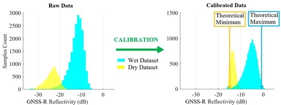
From the zones in the previous objective, verify the potential and capacity of desert areas to obtain a calibration bias parameter using GNSS-R reflectivities.
(c)
Once the bias parameter is estimated, verify the suitability of a scale factor based on wetlands’ reflectivity, according to the method proposed by [25].
(d)
To perform the conversion of calibrated GNSS-R reflectivities into SMC values.
(e)
To validate the SMC values estimated from the calibrated reflectivities.
Areas fulfilling the prerequisites of (a) are described in the next section, in terms of biome classes, BSR, and VOD. To accomplish (b) and (c) objectives, the GNSS-R reflectivity values are obtained from the data acquired by the CYGNSS mission; the CYGNSS data are described in Section 2.3. To satisfy objective (d), we employ the converted Fresnel linear reflectivity coefficients from the calibrated GYGNSS reflectivity estimates to estimate SMC. This is possible for low incidence angles, as was pointed out by [17,27]. The methodology for SMC retrieval, along with our proposed method for CYGNSS reflectivity calibration, are described in Section 3. Then, the theoretical dielectric properties of wetlands and deserts, and the analysis and calibration of CYGNSS reflectivity from the calibration areas are presented in Section 4. Under these conditions, our results will show the potential capacity of the inversion procedure and highlight the conditions for a correct assessment of SMC. To achieve the last objective of this approach, the specific geographical areas are tested using the existing SMAP SMC products. The validation of the CYGNSS SMC estimates with the SMAP SMC products is presented in Section 4.3. The final discussion and conclusions are given in the last sections.

2. Study Areas and Data

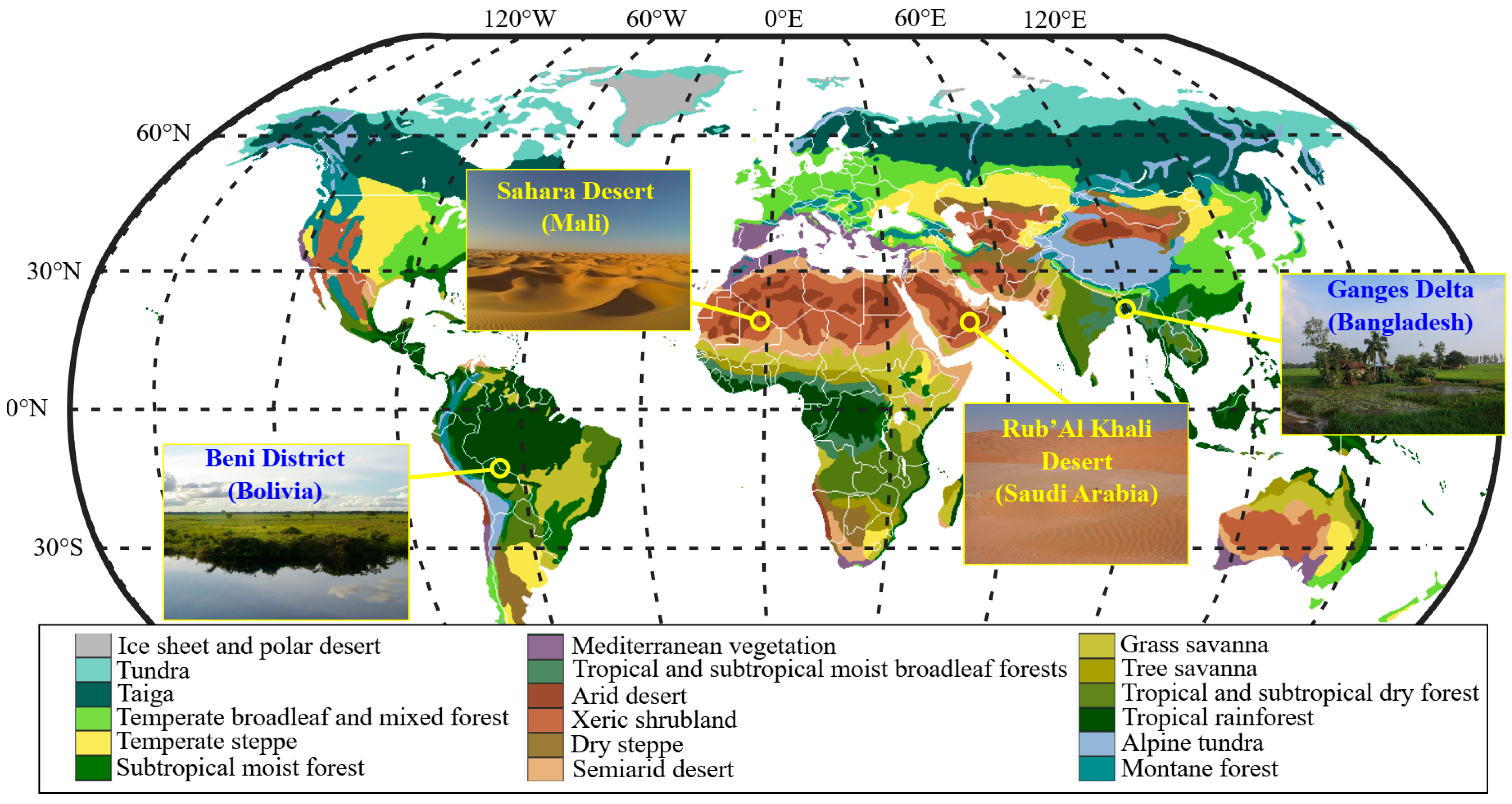
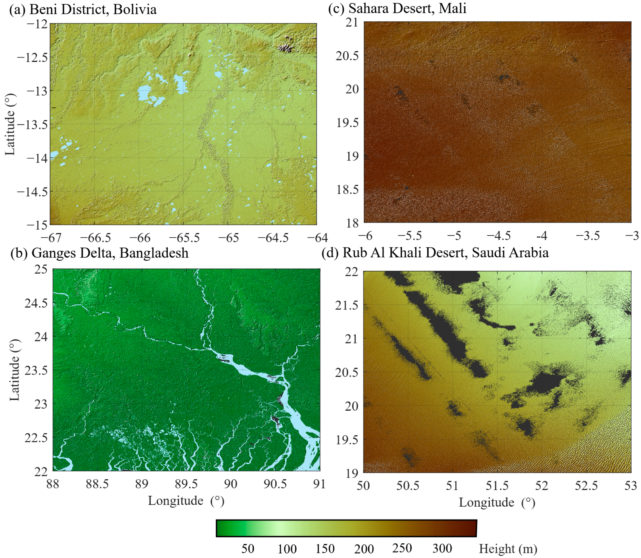
2.1. Calibration Areas

To achieve the objectives proposed in this study, two different areas for wetlands and deserts were selected, for both calibration and validation procedures. This step corresponds to objective (a) described in the Introduction Section. These 4 zones are shown in Figure 1, and the coordinates of the corners are listed in Table 1. Concerning the calibration values based on reflectivity from wetlands, the GNSS-R data comply with certain characteristics as follows. Large wetland areas are selected in order to contain a high number of water bodies so that the probability of identifying a significant number of specular points at water surfaces is very high.
Two zones are located in tropical rainforest biomes, one in Bolivia and the other in Bangladesh. The other two zones are located in desert biomes, one in the Sahara and the other in Saudi Arabia. For this purpose, some conditions are considered as follows. The dry areas are selected falling in the arid category [29]. For these areas to be used for calibration and validation purposes, and to ensure optimal SMC conditions, the months with minimum rainfall are used. According to [30], the average rainfall in the western and eastern areas of the Sahara Desert, along the 20°N parallel, is practically null. Similar areas can also be identified in the Arabic peninsula [31]). These zones are shown in Figure 1. To ensure the quality of the CYGNSS data, we employ specular points with heights below 700 m, as pointed out in the GNSS-R studies of [31,32]. The corresponding land surface heights from NASA’s Shuttle Radar Topography Mission (SRTM) data are shown in Figure 2.

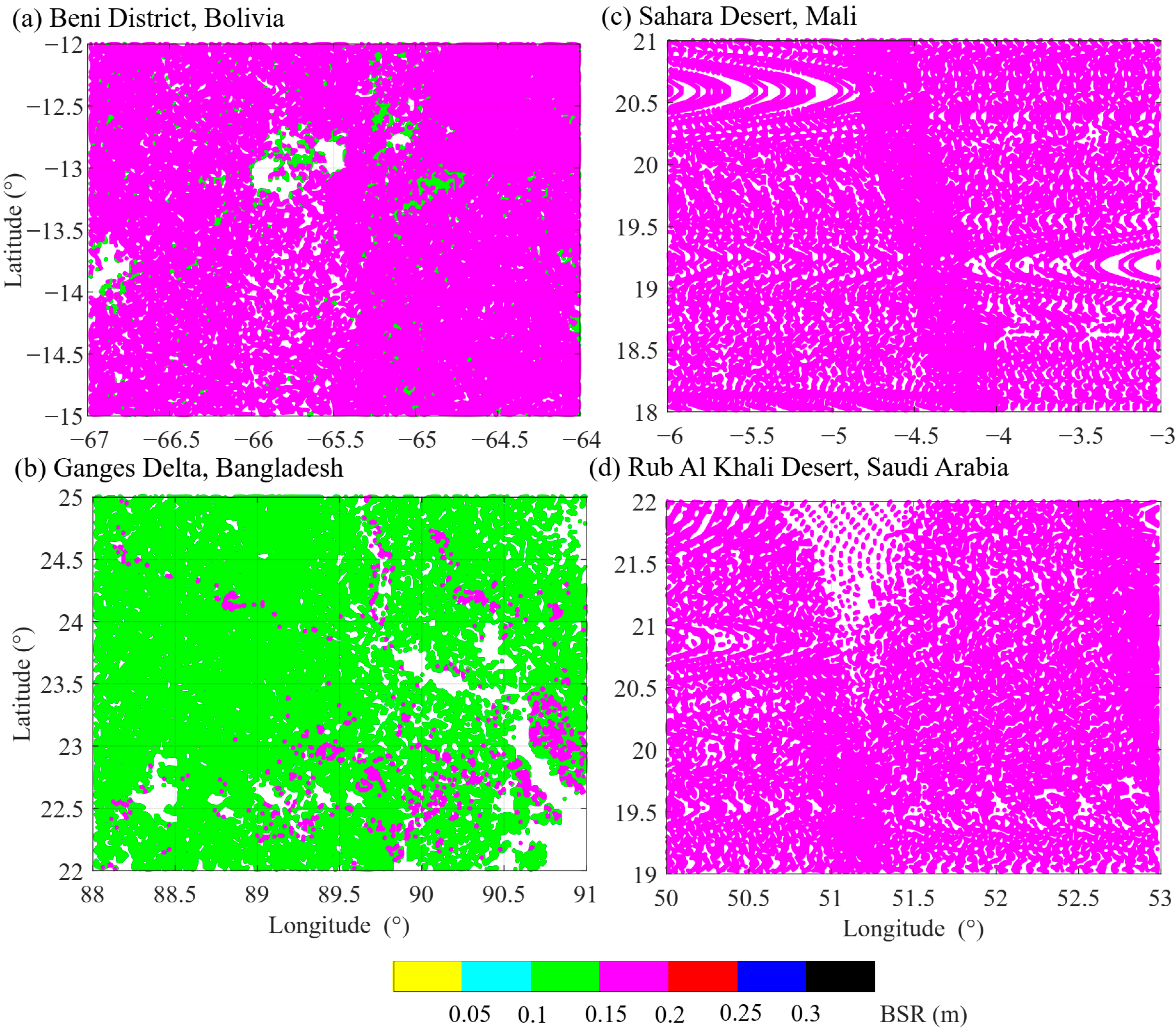
2.2. SMAP BSR, VOD, and SMC Data from the Calibration Areas

Concerning objective (a) described in the Introduction Section, the SMAP/Sentinel-1 L2 Radiometer/Radar at 30-s Scene and 3 km EASE-Grid Soil Moisture (Version 2) product [34] provides BSR and VOD estimates along with other parameters, e.g., SMC for the first 5 cm of surface depth, volumetric water content, etc. In this work, we employ SMAP SMC estimates as reference true values for validating our GNSS-R SMC retrieval technique (see Section 4.3). SMAP products are available at [34]. Figure 3 and Figure 4 show the SMAP BSR and VOD estimates, respectively, for July and August of 2021. For the selection of the calibration zones, we take into account a very low BSR, as suggested by [31]. The SMAP BSR values for the 4 calibration areas are shown in Figure 3, showing values below 0.3 m, and, specifically, the zone of Bangladesh shows values below 0.15 m. The values of VOD from SMAP are shown in Figure 4. As expected, the desert areas have practically null VOD, while the wetlands show a larger range with a variety of values. High VOD values (>0.9) are observed in some areas of Bolivia, specifically at high altitudes, as we can identify in Figure 2. The VOD values are below 0.45 in the center of the figure. Notwithstanding, the possible effects due to VOD attenuation will not influence our calibration procedure, since our method employs the 99% quantile of the data (see next section). On the other hand, the Bangladesh area shows, in general, lower VOD values than that seen in Bolivia, with VOD values below 0.45 in practically all scenes. The low VOD and BSR values for the area of Bangladesh results in an excellent area for calibration purposes.

2.3. CYGNSS Data

The CYGNSS mission of NASA is the most recent Earth-observing GNSS-R constellation; it consists of 8 satellites launched onboard a Pegasus XL Rocket on 15 December 2016 (online measurements are available from March 2017 at [35]). The CYGNSS satellites are located in an equatorial orbit with an inclination of 35° at about 500 km altitude. The initial research objectives of CYGNSS were the observation of tropical cyclones, so the coverage is limited to low and middle latitude ranges (38°S to 38°N). However, the land surface scattered signals have provided an unprecedented opportunity to study BSR and dielectric properties [18,19,23]. The CYGNSS data will be used to cover objective (b) described in the Introduction.
In CYGNSS, the geometry of observation follows a bistatic configuration [36]. Each CYGNSS satellite is equipped with a GNSS up-looking RHCP antenna and two GNSS down-looking LHCP antennas. These antennas are categorized as bistatic radar receivers at the L-band (L1-band frequency at 1.57542 GHz), namely DDM instruments. These instruments are designed to map the scattered signal on the oceans and land surfaces, which are sampled in time and frequency, thus delivering DDMs at the proximity of the specular point. These DDM instruments compute 4 measurements every second, which are compressed and downloaded to the ground processing facilities [19]. There are 3 CYGNSS processing levels freely available to the scientific community, ranging from level 0 to 3, and subsequent sub-levels. In this study, we employ level-1 data, which contains geo-located DDMs calibrated into an ideal (analog) power sensor (PDDM). Additional level-1 parameters are required in this study; these include DDM timestamp, latitude (φSP), longitude (λSP), incidence angle (θSP) of the specular points (SP), antenna transmitter gain (Gr), GPS effective isotropic radiated power (EIRP), and ranges from the receiver (Rr) and transmitter (Rt) antennas. The CYGNSS DDM data specifications and processing schemes are given in [37,38,39]. The transmitter power (Pt) and gain (Gt) of the antenna, as well as the gain of the receiver antenna (Gr) in the direction of the specular point, are available in the L1 CyGNSS product file.
The geometric distribution of the observed specular points follows a quasi-random spatiotemporal distribution, due to the changing geometry of the GNSS and CYGNSS satellites [23]. This distribution is very different from the conventional data delivered by active/passive microwave instruments onboard satellites. Therefore, the challenge includes a very different condition from the first Fresnel ellipses (areas of specular points), because the distances between the transmitter and the receiver differ considerably from one observation to another. In addition, the size of the specular points varies according to other factors, including the incidence angle and the height of the receiver [36,40,41]. The authors in [19] quantified a mapping resolution near 150 m depending on the observation geometry. The authors in [42] assessed the spatial resolution of the coherent Fresnel reflection zone to approximately 0.65 × 0.85 km2, also depending on the above factors. The CYGNSS data used in this study range from July to August of 2021, and we apply the following filter criterion, e.g., [31], for quality purposes:
(1)
CYGNSS reflectivity values range between −35 dB and −5 dB;
(2)
Incidence angles range between 0° and 25°;
(3)
DDM signal-to-noise ratio (SNR) is greater than 3 dB;
(4)
Gr (receiver antenna gain towards the specular point) is greater than 5 dB;
(5)
Land surface heights are lower than 700 m.
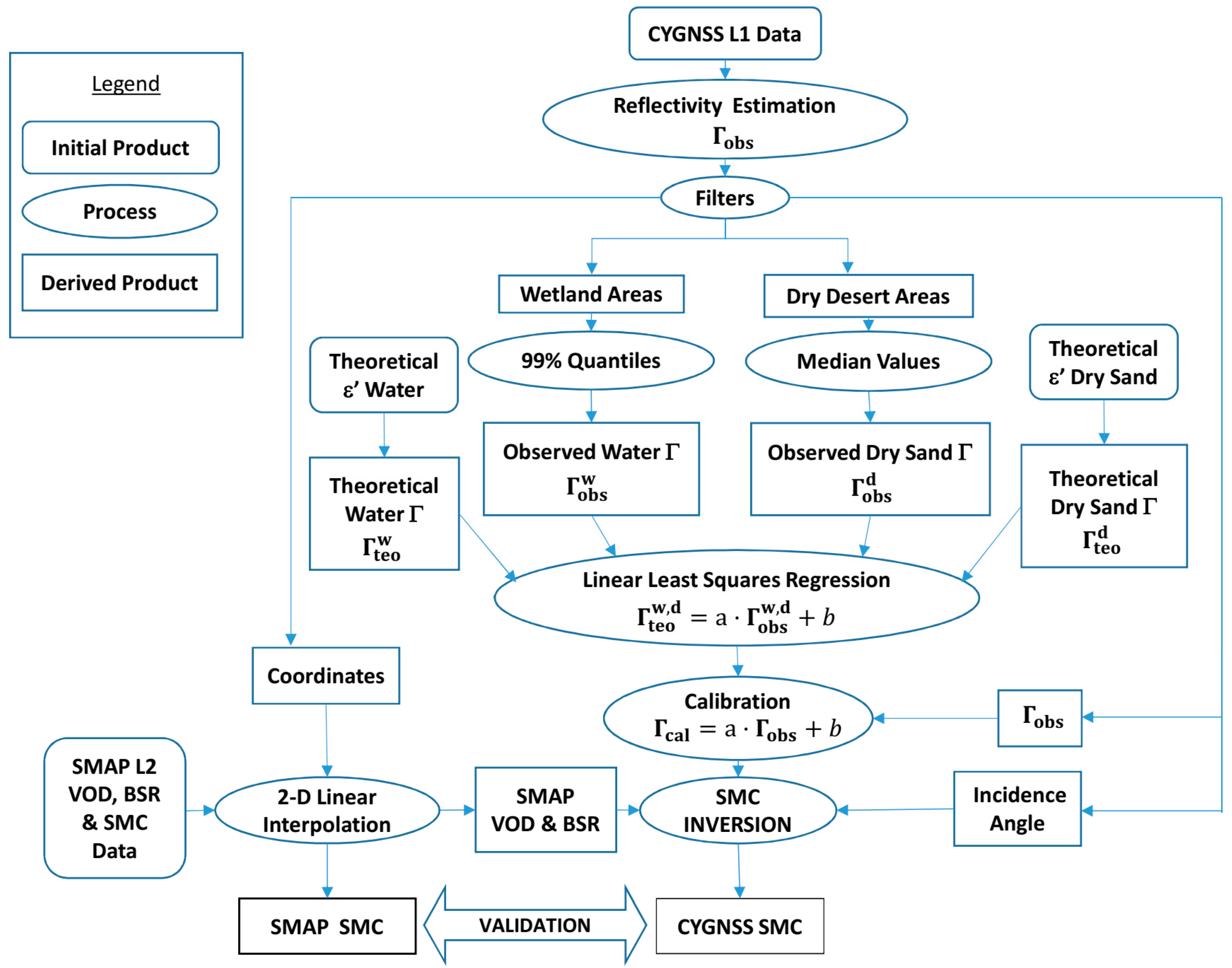
3. Methodology

After covering the first objective, (a), described in the previous section, the following methodology proposed is divided into two parts. First, the reflectivities of water and deserts are calculated for the specular points obtained by the eight CYGNSS satellites. The data are filtered for the calibration areas indicated in Figure 1 and Table 1. Then, in the second part, the derived CYGNSS reflectivity values are contrasted with theoretical water and dry sand reflectivity values. This step corresponds to objectives (b) and (c) described in the Introduction.
To compute CYGNSS reflectivity values, we only consider the strongest scattering power provided by natural land surfaces, which is received from the coherent part of the reflected signal [19,43]. In this sense, land surface reflectivity can be sensed from GNSS-R data through the bistatic radar equation for the coherent component of LHCP GNSS bistatic microwave signals [17,36,44,45,46], which takes the following expression [20] when dealing with GNSS-R data:
Γ lr ( θ ) = ( 4 π ) 2 ( P DDM N ) ( R t + R r ) 2 λ 2 G t G r P t
In this equation, PDDM is the DDM peak value from the analog scattered power. The subscript lr stands for a scattering mechanism when the incident RHCP signal is scattered by the surface and inverts the polarization to LHCP at the receiver position. Γlr is the surface reflectivity from which the SMC might be estimated, after correction of the noise floor component (N) in the DDM [31,46]. Rt and Rr are the transmitter and receiver range to the specular point, respectively. Gt ·Pt is the transmitter equivalent to isotopically radiated power (EIRP). Gr is the receiver antenna gain in the direction of the specular point. λ is the wavelength of the system, and θ refers to the incidence angle of the signal. Note that θ is constrained for angles range between 0°and 25° as indicated in the previous section.
For each specular point, the values for the variables (PDDM, Pt, Rt, Rr, Gt, and Gr) involved on the right side of Equation (1) are available at the CyGNSS L1 product, and they are crucial for calculating the CyGNSS measured reflectivity Γlr. Moreover, as the scattered analog power (PDDM) is affected by a system noise N, it must be corrected by this effect, as mentioned before. The parameter N is estimated from a subset of the DDM where no signal, above the horseshoe shape of the DDM [20], is present. The above equation is the final expression for a CYGNSS specular point reflectivity or measured reflectivity Γlr.
Furthermore, Γlr needs to be calibrated from instrumental bias and corrected for surface roughness and vegetation effects, as explained as follows. For any surface in general, but in particular for land surfaces, the inherent BSR and VOD affect the observed reflectivity [21], and are defined as follows:
BSR ( k , σ , θ ) = e ( 2 k σ cos θ ) 2 VOD ( τ , θ ) = e 2 τ / ( cos θ ) 2 }
where τ stands for the VOD and k = 2π/λ. Here, λ is the wavelength of the GNSS system, and σ is the standard deviation of the surface roughness. These variables are found in [34]. Then, the implementation of the BSR and VOD effects in Equation (1) is as follows [17,21,22,27,34,36]:
| R lr ( θ ) | 2 = Γ lr ( θ ) BSR ( k , σ , θ ) VOD ( τ , θ )
In this equation, Rlr is the Fresnel reflection coefficient identified as the surface reflectivity without BSR and VOD effects. The subscripts lr and rl stand for circular cross-polarized reflections. Rlr is required for extracting the soil moisture parameter, which is obtained through inversion of Equation (3). For this study, as we employ smooth surfaces, the BSR component can be avoided. Moreover, for some wide desert areas, vegetation attenuation effects can also be omitted.
Then, since the reflectivity for theoretical water and dry sand dielectric constants values can be determined using the Fresnel reflection coefficients (Rvv and Rhh), we can relate them to the Rlr and Rlr reflectivity circular polarization modes as follows [17,27,36,40]:
R rl = R lr = 1 2 ( R vv R hh )
where the subscripts vv and hh stand for vertical and horizontal polarization, respectively. Note that the variables in Equation (4) are function of θ. The dielectric constant of the land surface (εr), and incidence angle of the signal (θ) are the variables defining the Fresnel reflection coefficients. Expressions for these coefficients are found in many works (e.g., [21,47]), and references therein). An important point in this context is the use of low incidence angles θ ≤ 25°, where the difference between the reflections’ coefficients for vertical and horizontal polarization can be considered negligible [17,40]. Therefore, under these circumstances, the Fresnel equations can be solved either for one of these two coefficients. Thus, by expressing Equation (3) in terms of Equation (4), the reflectivity of a land surface sensed by GNSS-R can be calibrated using empirically estimated dielectric constants.
The second part of this methodology involves the calibration of the observed CYGNSS reflectivity values (Γobs) obtained with Equation (3). This step corresponds to objectives (b) and (c) described in the introduction. For this purpose, we employ the following parameterization to obtain calibrated reflectivity values (Γcal):
Γ cal = a Γ obs + b
where the bias parameter b is estimated from the minimum reflectivity values, specifically those obtained from deserts, which theoretical reflectivity is approximately 0.06 (−12 dB). The scale factor a is estimated from the maximum reflectivity values, specifically those obtained from water bodies in the wetlands, whose theoretical reflectivity is approximately 0.348 (−1.96 dB). These theoretical values are deduced in Section 4.1. For a correct determination of these parameters, we first perform a statistical analysis of the retrieved surface reflectivity without calibration, considering the possibility of excluding outliers, if present, and other possible dependences accounting for the different GNSS Pseudorandom Noise (PRN) IDs and the different CYGNSS satellites. In the next step, we estimate the median and the 99% quantile of the observed reflectivity data for deserts and wetlands, respectively, and estimate the calibration parameters using Equation (5) in the linear least square fit. In this way, the bias parameter b is constrained by the deserts’ reflectivity, and the scale factor a is constrained by the wetlands’ reflectivity. Subsequently, accounting for 99% of the data, the minimum and maximum values of the calibrated reflectivity will correspond to the theoretical reflectivity of the dry sand and the water bodies, respectively. Finally, we apply the calibration parameters to the reflectivity values following Equation (5) and estimate CYGNSS SMC with the ancillary BSR and VOD data from SMAP following the SMC inversion method of [21]. This step corresponds to objective (d) described in the Introduction Section. Then, for objective (e) described in the Introduction Section, the validation of the new CYGNSS SMC estimates can be achieved by comparison to the SMAP SMC estimates.
In brief, the methodology for the calibration of GNSS-R reflectivity is summarized in Figure 5. Starting with the available L1 data from CyGNSS, the observed reflectivity (Γobs) for both wet and dry datasets is estimated with Equation (3). Then, the “Filters” are those described in Section 2, including the limits of the study areas, altitude of the specular points, incidence angles, etc. This filtering provides the observed reflectivity for wetlands and deserts, their incidence angles, and the coordinates of each specular point. Then, the observed reflectivity data of wetlands and deserts are used to obtain the calibration parameters as detailed above, using the 99% quantile and mean, respectively, in the least square regression. These parameters are used to calibrate the observed reflectivity data from any location on Earth. The resulting reflectivity values are used to estimate SMC with ancillary data of VOD and BSR. Finally, the validation is performed with external data sources, for example, SMAP SMC. Note the ancillary data points and the CyGNSS specular point are not coincident, and therefore a 2D linear interpolation is required.

4. Results and Discussion

4.1. Theoretical Water/Dry Soil Dielectric Properties

The interactions of electromagnetic fields with materials are described through the fundamental electrical property, namely the relative permittivity of material (ε). This value is a complex quantity with real and imaginary components given by the following equation:
ε = ε j ε
where ε′ and ε″ are the real component of ε, also called the dielectric constant, and the imaginary component, referred to as the dielectric loss factor, respectively. The real part of the permittivity represents the ability of the materials to store electric energy. Microwave remote sensing is mainly focused on this component, as it allows us to derive an estimate of the water content in materials such as soil or vegetation. In the case of water, it allows for characterizing the chemical composition and thermodynamic properties. Dielectric properties of water and soils are generally well known [48,49,50,51]. For these both types of materials, several authors have addressed relevant physical characteristics revealing different behaviors to various physical parameters, such as temperature and frequency, as well as to other constituent contents, like salinity and sediments (e.g., [52,53,54]).
For water bodies, the driving variables are temperature and frequency [55,56,57]. The effects of these two variables on the dielectric constant are shown graphically in Figure 6a; these values are derived from the model [56]. In this study, the measurements are acquired at a fixed frequency (1.57542 GHz). The water temperature is assumed to be 20 °C. Other effects including temperature variability and roughness must be revised in future studies. For soils, several authors have thoroughly addressed the different behaviors of the dielectric constant to various physical parameters (e.g., [48,51,58,59,60,61]). While soils are largely affected by textural and moisture conditions, in the 1–1.6 GHz range, the dielectric properties of dry soils remain unchanged [62]. Moreover, in the absence of liquid water, the microwave dielectric constant of soils lacks significant dependencies on either temperature or frequency. The dielectric properties of dry soils are only dependent on the soil bulk density. In general, due to the soil bulk density, the real part of the dielectric constant for dry sandy soils might vary between 2.0 and 4.0. The authors of [49] empirically related the real component of soil permittivity to bulk density by the following expression:
ε soil = ( 1 + 0.44 ρ b ) 2
where ρb is the bulk density of the soil. Figure 6b shows the effects of bulk density on the dielectric constant of three soils with different water content (SMC units are cm3/cm3). Usually, the bulk density of the soil varies between 1.1 and 1.9 g/cm3 [63]. In this work, we referred to the online tool soil bulk density from the Global Gridded Surfaces of Selected Soil Characteristics [64] database. The soil bulk density for the deserts is identified as 1.6 g/cm3. The corresponding dielectric constant value is 2.904; this value is computed using Equation (7). The other values for constants under SMC of 0.1 and 0.2 in Figure 6b are computed using the model of [45]. Note that the dielectric constant considerably increases with SMC, as compared to increases due to bulk density variability. Another factor influencing the dielectric behavior of these materials is the effect of the observation angles. Figure 7 shows the reflectivity for different incidence angles and different dielectric constant values, where the reflectivity values start being affected for incidence angles above 45° [65,66]. Under these cases, following Figure 7, wet soils provide theoretical reflectivity values ( Γ teo w ) above −4 dB, and dry sandy soils ( Γ teo d ) are approximately between −15 dB and −8 dB. On the one hand, we use a theoretical dry sand reflectivity value of −12 dB. This value is in accordance with the permittivity value of 2.904 within the 0° to 25° incidence angle range. On the other hand, we employ −1.96 dB for the theoretical reflectivity of water, which is in accordance with theoretical reflectivity value of pure water at 20 °C. Note these values are for the GNSS frequency of CyGNSS (L1-band frequency at 1.57542 GHz).

4.2. Analysis and Calibration of CYGNSS Reflectivity

The statistical analysis of the retrieved surface reflectivity without calibration for the different GNSS PRN IDs and the different CYGNSS satellites is shown in Figure 8. The central marks indicate the median values, and the bottom and top edges of the boxes indicate the 25th and 75th percentiles, respectively. The whiskers extend to the most extreme data points that are not considered outliers, and the outliers are plotted individually using the ‘+’ symbol. In this figure, we can observe that the different satellites provide similar reflectivity responses for each of the calibration areas. As expected, the deserts provide lower values than the wetlands. In each case, we can observe no very consistent biases for the different GNSS PRN IDs (e.g., PRN 15 shows different biases between Bolivia and Bangladesh), while the different CYGNSS satellites provide lower variability. Notwithstanding, few outliers are observed, and the calibration of these biases will be addressed in future research with a large amount of data.
The statistics of quantile 99% for the wetlands and median average for the deserts are shown in Table 2, and the results of the least square estimation provided a bias parameter of b = 0.018, and a scale factor of a = 3.77. Similar to Figure 8, Figure 9 provides the reflectivity values after applying these calibration parameters with Equation (5). In this figure, we can observe all the reflectivity values were rearranged according to wet and dry constraints specified in Section 3. The quantile 99% of the wetlands data reaches −1 dB, and the deserts are between −15 dB and −8 dB, as implemented by the constraints. Although Figure 8, Figure 9 and Figure 10 show reflectivity values expressed in decibels (dB), the calibration adjustment procedure must be performed using decimal reflectivity values, as detailed in the previous section. In Figure 10, the histograms of the reflectivity estimates before and after calibration are presented for each calibration area. In this figure, we can better observe that the reflectivity values have shifted to higher ranges. For instance, in the case of desert areas, we can observe nearly coincident mean values for the calibrated data.

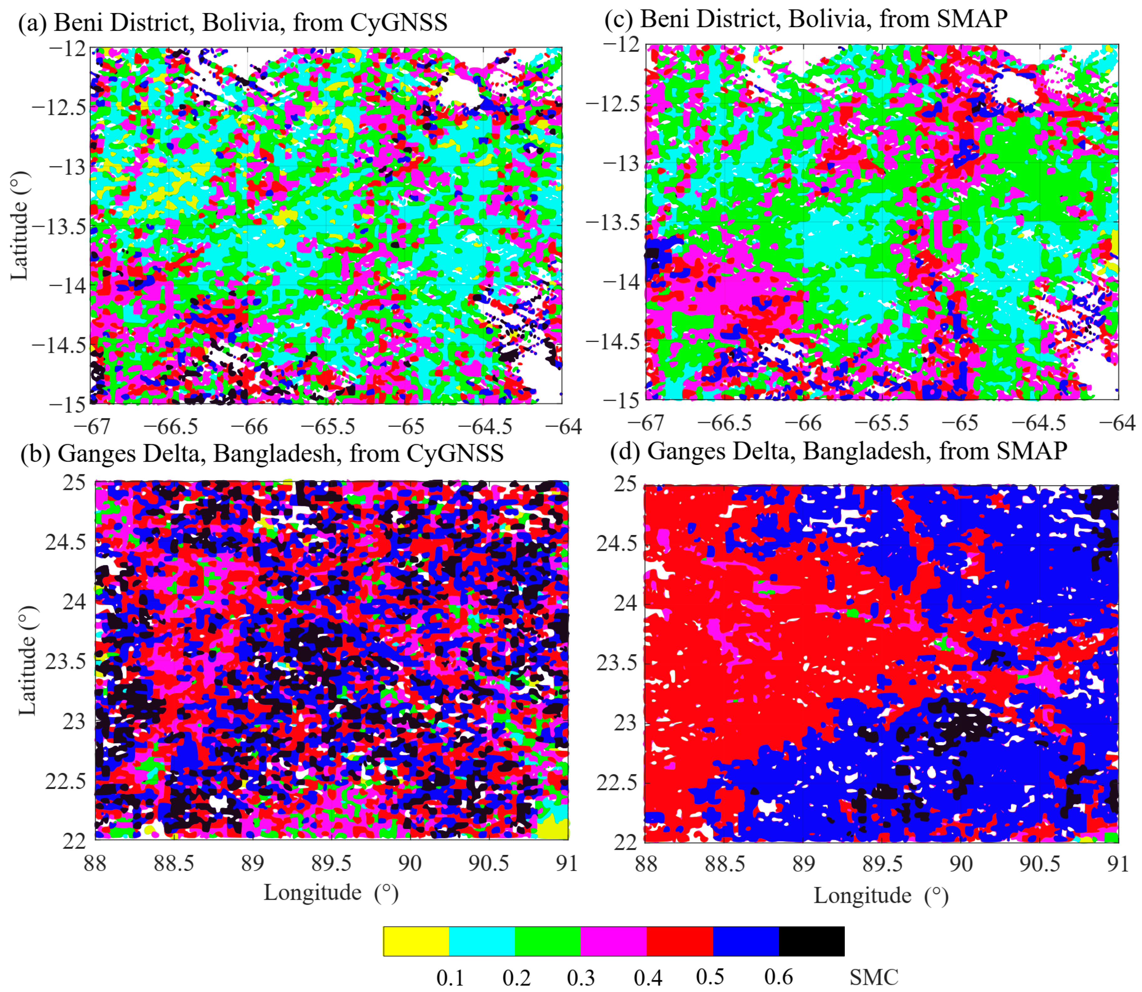
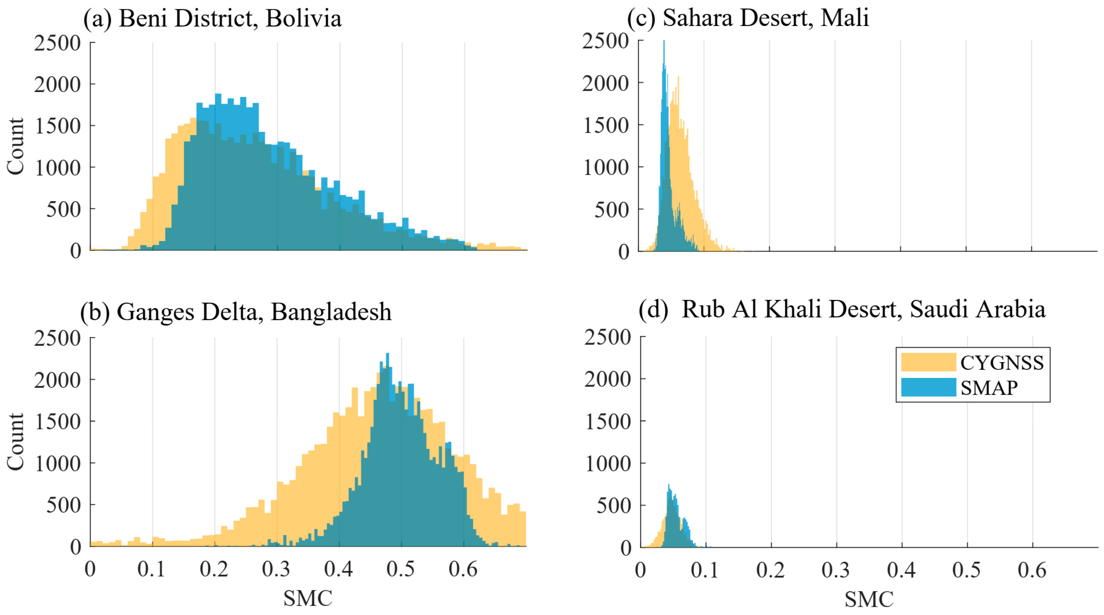
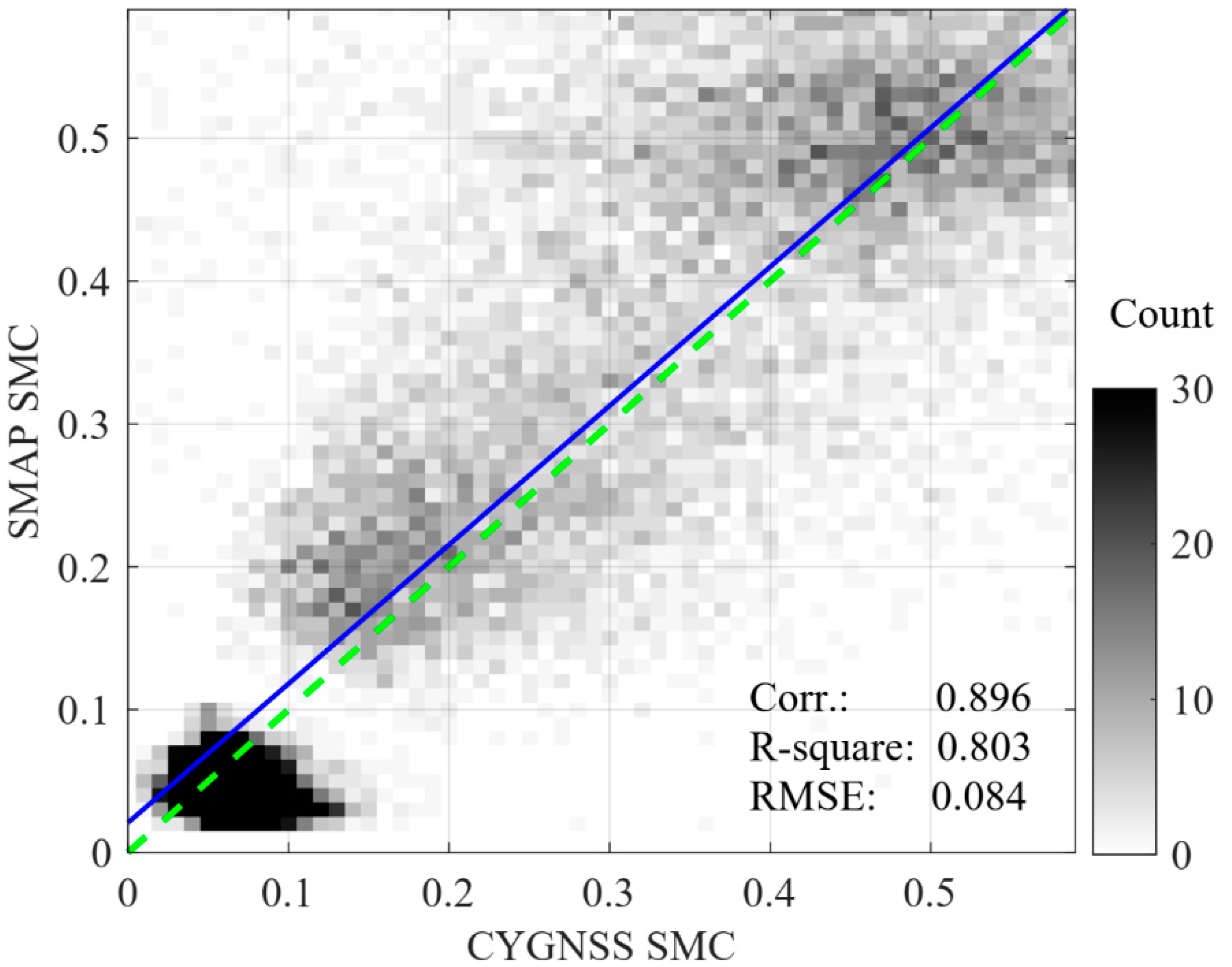
4.3. Validation of CYGNSS SMC with SMAP SMC

Our validation process is carried out by comparing the SMC retrieved from CYGNSS calibrated reflectivities with the SMAP SMC products. We directly employ the SMC inversion models as indicated in the literature [17,21,27,36,40,68,69], and with no additional adjustments. Although corrections due to VOD attenuation were only necessary for wetlands, we corrected BSR and VOD for all four calibration areas. In the desert areas, the VOD correction was minimum due to the lack of vegetation. Regarding the BSR contribution, the low values shown in Figure 3 generate negligible attenuations because of the system frequency used in GNSS, as suggested in [21]. However, the significance of VOD values is rather diverse for wetlands (Figure 4).
The calibrated CYGNSS reflectivity values for the four test areas are converted to SMC according to the indications in the previous section. Figure 11 and Figure 12 show the SMC estimates for desert and wet areas, respectively. In general, the SMC estimates from calibrated GyGNSS reflectivity values are in very good accordance with SMAP SMC.
For instance, at first, note the great differences between the SMC ranges when comparing desert and wetlands, i.e., Figure 11 and Figure 12, respectively. The GyGNSS and SMAP SMC ranges are in very good accordance. Concerning the dry areas, in the Arabian Desert (Figure 11b,d), most of the estimates are below 0.1 SMC, and a small number of samples between 0.1 and 0.2 in SMC can be observed in both GyGNSS and SMAP products near 20.5°N 51°E. For the Sahara Desert (Figure 11a,c), most of the estimates are below 0.1 SMC, while some small deviations to SMAP are observed in the northern areas. Concerning the wet areas, in Bangladesh (Figure 12b,d), most of the estimates are above 0.4 SMC, and a small number of samples between 0.3 and 0.3 in SMC can be observed in both GyGNSS and SMAP products near 245°N 88.5°E. For Bolivia, very clear and well-defined structures of enhanced SMC are observed in both SMAP and CYGNSS products, mostly along the river at the meridian 65°W, as well as in other minor elongated structures, e.g., in the northwest and southwest regions, etc. Our CYGNSS SMC provides excellent results in Bolivia.
The histograms of SMC from both SMAP and CYGNSS products are shown in Figure 13. This figure shows the statistical comparison of the extracted SMC from the CYGNSS calibrated reflectivity values and the SMAP SMC product. We can appreciate the ranges for CYGNSS are in very good accordance for all four calibration areas. In this figure, a slightly broader range is seen from CYGNSS. This may be the influence of the PNR dispersion due to signals from different GNSS satellites (Figure 8 and Figure 9). Figure 14 shows the linear fit between the retrieved CYGNSS and the SMAP SMC for all the data used in this study (four test areas from July to August 2021). In this figure, three clusters are distinguished, corresponding to the desert areas, and the two wetlands; the right uppermost cluster corresponds to the Bangladesh area. Pearson’s correlation coefficient reaches 0.89, and the standard linear regression statistics are R-square of 0.803 and root mean square (RMSE) of 0.084. The relevance of these results shows the good agreement between the retrieved values of SMAP and CYGNSS SMC, which emphasizes the good performance of the applied calibration method, as well as the correct conversion of calibrated CYGNSS reflectivity into SMC through the Fresnel coefficients method, as pointed out in [21].

4.4. Discussion

Calibration of GNSS-R reflectivity is an important step that must be accomplished to provide correct values that can be converted into accurate estimates of physical or biophysical variables. Different studies have addressed the issue of calibrating GNSS-R reflectivity estimates. However, these studies were incomplete or not well-raised (e.g., [17,21,25]), or were based on regression approaches with no physical inversion models [20,23,24]). Among these studies, based on the results of several experiments and testing different areas in eastern China, Clarizia et al. [21] used a bias value of 0.15 to obtain “reasonable” correlations in SMC retrieval using GYGNSS reflectivity. However, for low reflectivity values such as deserts, a 0.15 increase in the reflectivity of these areas would produce unacceptable SMC values that were not detected in their study. Wan et al. [25] proposed an interesting calibration approach with water reflectivity observations, but the authors had to normalize their reflectivity data to estimate the scale factor parameters, which were fitted using decibel units. However, by estimating the scale factor in decibel units, an exponential fit to the reflectivity range is produced, and no bias parameter can be included, while the subsequent need for a second calibration scheme was required to achieve ‘reasonable’ correlations with ancillary SMC estimates. Other authors opted to employ regression approaches to ancillary SMC data, but the actual reflectivity values sensed by GNSS-R still remains unknown.
In this work, we developed a calibration method that employs water bodies’ and dry sand’s reflectivity values. The initial idea was to identify some areas on the Earth’s surface that contain extreme dielectric theoretical conditions. In addition to well-known factors, such as surface roughness or SMC for soil surfaces, the reflectivities of water and dry sand are also affected by many other factors that must be considered. When used for calibration purposes, the water temperature must be taken into account, as it is a driving factor that modifies seriously theoretical values of this variable. In this sense, a proper set of calibration references must be taken, such as water bodies, since these can exhibit a thermal homogeneous behavior. It was verified that the water dielectric properties differ substantially with temperature. Another inconvenience was the collection of statistically sufficient specular points in water bodies. This was a difficult task, due to difficulties in identifying suitable water bodies that comply with CYGNSS specular point requirements. Furthermore, saline waters are not appropriate for this purpose. In this work, we opt for a strategy that allows for extracting a higher number of specular points, which is based on the 99% quantile of the histogram of a wetland area. The resulting samples correspond to the values of maxima reflectivity and are supposed to agree with the specular points on water bodies and highly wet soils. Therefore, to ensure a representative number of specular points in water, two reference areas with similar temperatures were selected, a wetland area in the Bolivian Amazon, and a flooded area in Bangladesh. This methodology differs from other studies in which the water reflectivity values used for calibration were collected from rivers and other water bodies that could exhibit distinct temperature conditions leading to different water permittivity values, see, e.g., [25]. To this extent, a large sample of observed water reflectivity values could be extracted from the two designated wetlands.
The possibility of using dry sand’s reflectivities for calibration has not yet been fully explored. It is demonstrated that, in addition to SMC, bulk density is an important variable that affects its dielectric properties. In turn, the temperature is not a driving factor altering these properties. In this scheme, our starting hypothesis for considering this abiotic variable for calibration purposes was that under drought conditions, some large deserts are constituted by dry sand at 0% SMC. Under these circumstances, the main variable that governs the dielectric properties of dry sand is the bulk density. This variable can be accessed through different databases such as the Global Gridded Surfaces of Selected Soil Characteristics database (2005). The advantage of using desert areas is the minimum influence of SMC, VOD, and BSR that may attenuate the reflectivity sensed by GNSS-R. These test areas can be treated as quasi-specular surfaces. For both the Mali and Arabian deserts used in this study, the observed reflectivity values were very homogeneous. After calibration, the derived CYGNSS SMC estimates in the four test areas were compared to SMAP products (Figure 13a–d), and the results are excellent.
Our suggested calibration model is based on a linear least-squares adjustment using observed and theoretical reflectivity values, which differs substantially from previous calibration procedures [17,20,25,32]. Validating with SMAP the SMC values from the corresponding calibrated CYGNSS reflectivities of the four test areas (Figure 13), the results show excellent agreement between both datasets in all test areas. This extent is also verified by the regression analysis depicted in Figure 14, where a very good fit is observed between SMAP and CYGNSS SMC; Pearson’s correlation coefficient is 0.89. This method completely differs from the UCAR procedure to retrieve SMC in the “The CYGNSS/DDMI Level 3 soil moisture” [23,24], where a direct regression to match SMAP SMC was performed from the uncalibrated CYGNSS reflectivity. Although the authors obtained good correlations because of the tight coupling between SMAP SMC, the resulting product was not recovered from a physical inversion model. Here, in this work, the CYGNSS reflectivities are calibrated with test areas that provide estimated calibrated reflectivities. The conversion to SMC is carried out independently from the SMAP SMC product after a physical transformation of the calibrated CYGNSS reflectivities using the Fresnel coefficients, as described in [21].
Based on the presented results, this methodology has some shortcomings that must be reviewed and addressed in future work. First, improvements must be made in the selection of test areas. A better identification of wetlands exhibiting similar properties regarding water temperature must be ensured. For desert areas, a better examination of the areas must be achieved to ensure the complete absence of VOD and BSR. It would be worth having better datasets for bulk density in desert areas. However, for these zones, this may not be feasible in the near future. On the other hand, better knowledge of this variable would improve the characterization of dry sand in these environments. Regarding the SMC validation approaches, additional reliable reference datasets are necessary, such as the ‘International Soil Moisture Network’ [70]).
This work is based on the coherent component of the signal without considering the incoherent effects of BSR and VOD. This implies that this contribution should also be reviewed in future work. As a concluding remark, this work demonstrates the capacity and suitability of dielectric properties from deserts and wetlands for calibrating GNSS-R reflectivity data.

5. Conclusions

Calibrating GNSS-R land surface reflectivity data is necessary to accurately estimate geophysical variables, such as SMC, biomass, or freeze/thaw, which are essential for monitoring Earth’s climate and hydrological cycle. In this work, we calibrated the GYGNSS reflectivity data by applying both a bias and a scale parameter estimated from the theoretical reflectivity values of different calibration areas that provide maximum range limits of reflectivity, such as deserts and wetlands. We used the wetlands of Bolivia and Bangladesh, and the deserts of Sahara and Saudi Arabia, under convenient altitude, BSR, and VOD conditions. Our innovative calibration scheme set the bias parameter with the lowest possible reflectivity of deserts, and the scale factor was estimated by the 99% quantile of the wetlands data to match the highest possible reflectivity response, such as that of water bodies. The CYGNSS scale factor and the bias parameter resulted in a = 3.77 and b = 0.018, respectively. Finally, the calibrated CYGNSS reflectivity values were used to directly obtain SMC estimates through the inversion of the Fresnel coefficients, including the attenuation corrections due to BSR and VOD influences. Our CYGNSS SMC results provide an excellent correspondence with the SMAP SMC products (standard linear regression: R-square = 0.77, RMSE = 0.095; Pearson’s Correlation = 0.88). We may have scientifically established the ultimate calibration method of GNSS-R reflectivity data to be used for accurate SMC estimation.

Author Contributions

I.M. and A.C. materialized the initial concept though investigation of previous research, formulation of new theory and methodology, draft preparation, supervision of achieved results, and provided international academic exchange; X.W. and K.E. provided collaboration, revision tasks, and draft preparation; S.J. provided supervision, mentorship, funding support, and undertook revision tasks. All authors have read and agreed to the published version of the manuscript.

Funding

This research was funded by the R&D+I Program of the Universidad Politécnica de Madrid (Programa Propio UPM 2019), the Talent Start-Up Funding project of NUIST (A.C., Grant No. 1411041901010), the Jiangsu Natural Resources Development Special Project (Grant No. JSZRHYKJ202002), and the Strategic Priority Research Program Project of the Chinese Academy of Sciences (Grant No. XDA23040100).

Acknowledgments

Great appreciation is extended to ESA and NASA for providing the data access. Special thanks are given to the three reviewers for their constructive comments and helpful suggestions. Special thanks are provided to the team of Remote Sensing Journal for their excellent work and support to publish this manuscript.

Conflicts of Interest

The authors declare no conflict of interest.

References

  1. Kim, H.; Lakshmi, V. Use of Cyclone Global Navigation Satellite System (CyGNSS) Observations for Estimation of Soil Moisture. Geophys. Res. Lett. 2018, 45, 8272–8282. [Google Scholar] [CrossRef] [Green Version]
  2. Santi, E.; Paloscia, S.; Pettinato, S.; Fontanelli, G.; Clarizia, M.P.; Comite, D.; Dente, L.; Guerriero, L.; Pierdicca, N.; Floury, N. Remote Sensing of Forest Biomass Using GNSS Reflectometry. IEEE J. Sel. Top. Appl. Earth Obs. Remote Sens. 2020, 13, 2351–2368. [Google Scholar] [CrossRef]
  3. Jin, S.; Komjathy, A. GNSS reflectometry and remote sensing: New objectives and results. Adv. Space Res. 2010, 46, 111–117. [Google Scholar] [CrossRef] [Green Version]
  4. Wu, X.; Jin, S. GNSS-Reflectometry: Forest canopies polarization scattering properties and modeling. Adv. Space Res. 2014, 54, 863–870. [Google Scholar] [CrossRef]
  5. Masters, D.; Zavorotny, V.; Katzberg, S.; Emery, W. GPS signal scattering from land for moisture content determination. In Proceedings of the IEEE International Geoscience and Remote Sensing Symposium, Honolulu, HI, USA, 24–28 July 2000; pp. 3090–3092. [Google Scholar]
  6. Masters, D.; Axelrad, P.; Katzberg, S. Initial results of land-reflected GPS bistatic radar measurements in SMEX02. Remote Sens. Environ. 2004, 92, 507–520. [Google Scholar] [CrossRef]
  7. Chew, C.C.; Colliander, A.; Shah, R.; Zuffada, C.; Burgin, M. The sensitivity of ground-reflected GNSS signals to near-surface soil moisture, as recorded by spaceborne receivers. In Proceedings of the International Geoscience and Remote Sensing Symposium (IGARSS), Fort Worth, TX, USA, 23–28 July 2017; pp. 2661–2663. [Google Scholar]
  8. Ruf, C.S.; Chew, C.; Lang, T.; Morris, M.G.; Nave, K.; Ridley, A.; Balasubramaniam, R. A New Paradigm in Earth Environmental Monitoring with the CYGNSS Small Satellite Constellation. Sci. Rep. 2018, 8, 8782. [Google Scholar] [CrossRef] [PubMed] [Green Version]
  9. Egido, A.; Caparrini, M.; Ruffini, G.; Paloscia, S.; Santi, E.; Guerriero, L.; Pierdicca, N.; Floury, N. Global navigation satellite systems reflectometry as a remote sensing tool for agriculture. Remote Sens. 2012, 4, 2356–2372. [Google Scholar] [CrossRef] [Green Version]
  10. Egido, A.; Paloscia, S.; Motte, E.; Guerriero, L.; Pierdicca, N.; Caparrini, M.; Santi, E.; Fontanelli, G.; Floury, N. Airborne GNSS-R polarimetric measurements for soil moisture and above-ground biomass estimation. IEEE J. Sel. Top. Appl. Earth Obs. Remote Sens. 2014, 7, 1522–1532. [Google Scholar] [CrossRef]
  11. Camps, A.; Park, H.; Pablos, M.; Foti, G.; Gommenginger, C.P.; Liu, P.W.; Judge, J. Sensitivity of GNSS-R Spaceborne Observations to Soil Moisture and Vegetation. IEEE J. Sel. Top. Appl. Earth Obs. Remote Sens. 2016, 9, 4730–4742. [Google Scholar] [CrossRef] [Green Version]
  12. Jia, Y.; Savi, P. Sensing soil moisture and vegetation using GNSS-R polarimetric measurement. Adv. Space Res. 2017, 59, 858–869. [Google Scholar] [CrossRef]
  13. Gleason, S.; Hodgart, S.; Sun, Y.; Gommenginger, C.; Mackin, S.; Adjrad, M.; Unwin, M. Detection and processing of bistatically reflected GPS signals from low earth orbit for the purpose of ocean remote sensing. IEEE Trans. Geosci. Remote Sens. 2005, 43, 1229–1241. [Google Scholar] [CrossRef] [Green Version]
  14. Wu, X.; Song, Y.; Xu, J.; Duan, Z.; Jin, S.G. Bistatic scattering simulations of circular and linear polarizations over land surface for signals of opportunity reflectometry. Geosci. Lett. 2021, 8, 11. [Google Scholar] [CrossRef]
  15. Zavorotny, V.U.; Gleason, S.; Cardellach, E.; Camps, A. Tutorial on Remote Sensing Using GNSS Bistatic Radar of Opportunity. IEEE Trans. Geosci. Remote Sens. 2014, 2, 8–45. [Google Scholar] [CrossRef] [Green Version]
  16. Privette, C.V.; Khalilian, A.; Torres, O.; Katzberg, S. Utilizing space-based GPS technology to determine hydrological properties of soils. Remote Sens. Environ. 2011, 115, 3582–3586. [Google Scholar] [CrossRef]
  17. Jia, Y.; Savi, P.; Canone, D.; Notarpietro, R. Estimation of Surface Characteristics Using GNSS LH-Reflected Signals: Land Versus Water. IEEE J. Sel. Top. Appl. Earth Obs. Remote Sens. 2016, 9, 4752–4758. [Google Scholar] [CrossRef]
  18. Rose, R.; Gleason, S.; Ruf, C. The NASA CYGNSS mission: A pathfinder for GNSS scatterometry remote sensing applications. In Remote Sensing of the Ocean, Sea Ice, Coastal Waters, and Large Water Regions; International Society for Optics and Photonics: Amsterdam, The Netherlands, 2014; Volume 9240, p. 924005. [Google Scholar]
  19. Carreño-luengo, H.; Luzi, G.; Crosetto, M. Sensitivity of CyGNSS Bistatic Reflectivity and SMAP Microwave Radiometry Brightness Temperature to Geophysical Parameters Over Land Surfaces. IEEE J. Sel. Top. Appl. Earth Obs. Remote Sens. 2018, 12, 107–122. [Google Scholar] [CrossRef]
  20. Clarizia, M.P.; Pierdicca, N.; Costantini, F.; Floury, N. Analysis of CyGNSS Data for Soil Moisture Retrieval. IEEE J. Sel. Top. Appl. Earth Obs. Remote Sens. 2019, 12, 2227–2235. [Google Scholar] [CrossRef]
  21. Calabia, A.; Molina, I.; Jin, S.G. Soil Moisture Content from GNSS Reflectometry using Dielectric Permittivity from Fresnel Reflection Coefficients. Remote Sens. 2022, 12, 122. [Google Scholar] [CrossRef] [Green Version]
  22. Camps, A.; Vall·llossera, M.; Park, H.; Portal, G.; Rossato, L. Sensitivity of TDS-1 GNSS-R Reflectivity to Soil Moisture: Global and Regional Differences and Impact of Different Spatial Scales. Remote Sens. 2018, 10, 1856. [Google Scholar] [CrossRef] [Green Version]
  23. Chew, C.; Small, E. Soil Moisture Sensing Using Spaceborne GNSS Reflections: Comparison of CYGNSS Reflectivity to SMAP Soil Moisture. Geophys. Res. Lett. 2018, 45, 4049–4057. [Google Scholar] [CrossRef] [Green Version]
  24. Chew, C.; Small, E. Description of the UCAR/CU Soil Moisture Product. Remote Sens. 2020, 12, 1558. [Google Scholar] [CrossRef]
  25. Wan, W.; Ji, R.; Liu, B.; Li, H.; Zhu, S. A Two-Step Method to Calibrate CYGNSS-Derived Land Surface Reflectivity for Accurate Soil Moisture Estimations. IEEE Geosci. Remote Sens. Lett. 2022, 19, 2500405. [Google Scholar] [CrossRef]
  26. Bindlish, R.; Barros, A.P. Parameterization of vegetation backscatter in radar-based, soil moisture estimation. Remote Sens. Environ. 2001, 76, 130–137. [Google Scholar] [CrossRef]
  27. Egido, A.; Ruffini, G.; Caparrini, M.; Martín, C.; Farrés, E.; Banqué, X. Soil moisture monitorization using GNSS reflected signals. In Proceedings of the 1st Colloquium Scientific and Fundamental Aspects of the Galileo Programme, Toulouse, France, 25–27 October 2007. [Google Scholar]
  28. Biome. Available online: https://en.wikipedia.org/wiki/Biome (accessed on 1 January 2022).
  29. Lim; Hwang; Kuang. The Sahara Desert Northern Africa. Available online: https://biomania-saharadesert.weebly.com/climatelocation.html (accessed on 15 January 2022).
  30. Henchiri, M.; Igbawua, T.; Javed, T.; Bai, Y.; Zhang, S.; Essifi, B.; Ujoh, F.; Zhang, J. Meteorological Drought Analysis and Return Periods over North and West Africa and Linkage with El Niño–Southern Oscillation (ENSO). Remote Sens. 2021, 13, 4730. [Google Scholar] [CrossRef]
  31. Stilla, D.; Zribi, M.; Pierdicca, N.; Baghdadi, N.; Huc, M. Desert Roughness Retrieval Using CYGNSS GNSS-R Data. Remote Sens. 2020, 12, 743. [Google Scholar] [CrossRef] [Green Version]
  32. Gleason, S.; O’Brien, A.; Russel, A.; Al-Khaldi, M.M.; Johnson, J.T. Geolocation, Calibration and Surface Resolution of CYGNSS GNSS-R Land Observations. Remote Sens. 2020, 12, 1317. [Google Scholar] [CrossRef] [Green Version]
  33. Beauducel, F. READHGT: Import/Download NASA SRTM Data Files (.HGT). MATLAB Central File Exchange. 2022. Available online: https://www.mathworks.com/matlabcentral/fileexchange/36379-readhgt-import-download-nasa-srtm-data-files-hgt (accessed on 1 February 2022).
  34. Das, N.; Entekhabi, D.; Dunbar, R.S.; Kim, S.; Yueh, S.; Colliander, A.; O’Neill, P.E.; Jackson, T. SMAP/Sentinel-1 L2 Radiometer/Radar 30-Second Scene 3 km EASE-Grid Soil Moisture, Version 2; 1 to 30 April 2019; NASA National Snow and Ice Data Center Distributed Active Archive Center: Boulder, CO, USA, 2018; Available online: https://nsidc.org/data/SPL2SMAP_S/versions/2 (accessed on 1 February 2022).
  35. OPeNDAP-PODAAC FTP Layout. Available online: https://podaac-opendap.jpl.nasa.gov (accessed on 1 September 2019).
  36. Jia, Y.; Pei, Y. Remote Sensing in Land Applications by Using GNSS-Reflectometry. In Recent Advances and Applications in Remote Sensing; Hung, M.-C., Wu, Y.-H., Eds.; IntechOpen: London, UK, 2018. [Google Scholar] [CrossRef] [Green Version]
  37. Gleason, S. Algorithm Theoretical Basis Document Level 1A DDM Calibration. In CYGNSS Level 1 Science Data Record Version 2.1; PO.DAAC: Ann Arbor, MI, USA; Cyclone Global Navigation Satellite System (CYGNSS): Pasadena, CA, USA, 2018. [Google Scholar]
  38. Gleason, S. Algorithm Theoretical Basis Document Level 1B DDM Calibration. In CYGNSS Level 1 Science Data Record Version 2.1; PO.DAAC: Ann Arbor, MI, USA; Cyclone Global Navigation Satellite System (CYGNSS): Pasadena, CA, USA, 2018. [Google Scholar]
  39. Ruf, C.; Chang, P.; Clarizia, M.P.; Gleason, S.; Jelenak, Z.; Murray, J.; Morris, M.; Musko, S.; Posselt, D.; Provost, D.; et al. CYGNSS Handbook Cyclone Global Navigation Satellite System: Deriving Surface Wind Speeds in Tropical Cyclones; National Aeronautics and Space Administration: Ann Arbor, MI, USA, 2016; p. 154. ISBN 978-1-60785-380-0. [Google Scholar]
  40. Katzberg, S.J.; Torres, O.; Grant, M.S.; Masters, D. Utilizing calibrated GPS reflected signals to estimate soil reflectivity and dielectric constant: Results from SMEX02. Remote Sens. Environ. 2005, 100, 17–28. [Google Scholar] [CrossRef] [Green Version]
  41. Qiao, X.; Khalilian, A.; Payero, J.O.; Maja, J.M.; Privette, C.V.; Han, Y.J. Evaluating Reflected GPS Signal as a Potential Tool for Cotton Irrigation Scheduling. Adv. Remote Sens. 2016, 5, 157–167. [Google Scholar] [CrossRef] [Green Version]
  42. Chew, C.; Lowe, S.; Parazoo, N.; Esterhuizen, S.; Oveisgharan, S.; Podest, E.; Zuffada, C.; Freedman, A. SMAP radar receiver measures land surface freeze/thaw state through capture of forward-scattered L-band signals. Remote Sens. Environ. 2017, 198, 333–344. [Google Scholar] [CrossRef]
  43. Ferrazzoli, P.; Guerriero, L.; Pierdicca, N.; Rahmoune, R. Forest biomass monitoring with GNSS-R: Theoretical simulations. Adv. Space Res. 2011, 47, 1823–1832. [Google Scholar] [CrossRef]
  44. Chew, C.; Reager, J.T.; Small, E. CYGNSS data map flood inundation during the 2017 Atlantic hurricane season. Sci. Rep. 2018, 8, 9336. [Google Scholar] [CrossRef] [PubMed]
  45. Wan, W.; Liu, B.; Zeng, Z.; Chen, X.; Wu, G.; Xu, L.; Chen, X.; Hong, Y. Using CYGNSS Data to Monitor China’s Flood Inundation during Typhoon and Extreme Precipitation Events in 2017. Remote Sens. 2019, 11, 854. [Google Scholar] [CrossRef] [Green Version]
  46. Rajabi, M.; Nahavandchi, H.; Hoseini, M. Evaluation of CYGNSS Observations for Flood Detection and Mapping during Sistan and Baluchestan Torrential Rain in 2020. Water 2020, 12, 2047. [Google Scholar] [CrossRef]
  47. Edokossi, K.; Calabia, A.; Jin, S.G.; Molina, I. GNSS-Reflectometry and Remote Sensing of Soil Moisture: A Review of Measurement Techniques, Methods, and Applications. Remote Sens. 2020, 12, 614. [Google Scholar] [CrossRef] [Green Version]
  48. Shahidi, M.; Hasted, J.; Jonscher, A. Electrical properties of dry and humid sand. Nature 1975, 258, 595–597. [Google Scholar] [CrossRef]
  49. Dobson, M.C.; Ulaby, F.T.; Hallikainen, M.T.; El-Rayes, M.A. Microwave Dielectric Behavior of Wet Soil-Part II: Dielectric Mixing Models. IEEE Trans. Geosci. Remote Sens. 1985, 23, 35–46. [Google Scholar] [CrossRef]
  50. Artemov, V.G.; Volkov, A.A. Water and Ice Dielectric Spectra Scaling at 0 °C. Ferroelectrics 2014, 466, 158–165. [Google Scholar] [CrossRef]
  51. Mätzler, C. Microwave permittivity of dry sand. IEEE Trans. Geosci. Remote Sens. 1998, 36, 317–319. [Google Scholar] [CrossRef]
  52. Cassidy, N.J. Chapter 2-Electrical and Magnetic Properties of Rocks, Soils and Fluids; Harry, M.J., Ed.; Ground Penetrating Radar Theory and Applications; Elsevier: Amsterdam, The Netherlands, 2009; pp. 41–72. ISBN 9780444533487. [Google Scholar] [CrossRef]
  53. Fitterman, D.V. 11.10-Tools and Techniques: Active-Source Electromagnetic Methods. In Treatise on Geophysics, 2nd ed.; Schubert, G., Ed.; Elsevier: Amsterdam, The Netherlands, 2015; pp. 295–333. ISBN 9780444538031. [Google Scholar] [CrossRef]
  54. Hallikainen, M. Microwave Dielectric Properties of Materials. In Encyclopedia of Remote Sensing; Encyclopedia of Earth Sciences Series; Njoku, E.G., Ed.; Springer: New York, NY, USA, 2014. [Google Scholar] [CrossRef]
  55. Speight, J.G. 2-The properties of water. In Speight, Natural Water Remediation, Butterworth-Heinemann, James, G., Ed.; Elsevier: Amsterdam, The Netherlands, 2020; pp. 53–89. ISBN 9780128038109. [Google Scholar] [CrossRef]
  56. Meissner, T.; Wentz, F.J. The complex dielectric constant of pure and sea water from microwave satellite observations. IEEE Trans. Geosci. Remote Sens. 2004, 42–49, 1836–1849. [Google Scholar] [CrossRef] [Green Version]
  57. Vijay, R.; Jain, R.; Sharma, K.S. Dielectric Spectroscopy of Grape Juice at Microwave Frequencies. Int. Agrophysics 2015, 29, 239–246. [Google Scholar] [CrossRef] [Green Version]
  58. Fano, W.G.; Trainotti, V. Dielectric properties of soils. In Proceedings of the 2001 Annual Report Conference on Electrical Insulation and Dielectric Phenomena (Cat. No. 01CH37225), Kitchener, ON, Canada, 14–17 October 2001; pp. 75–78. [Google Scholar] [CrossRef]
  59. Mätzler, C.; Murk, A. Complex Dielectric Constant of Dry Sand in the 0.1 to 2 GHz Range; Research Report No. 2010-06-MW.; Institute of Applied Physics, University of Bern: Bern, Switzerland, 2010. [Google Scholar] [CrossRef]
  60. Calla, O.P.N. Study of the properties of dry and wet loamy sand soils at microwave frequencies. Indian. J. Radio Space Phys. 1999, 28, 109–112. [Google Scholar]
  61. Ulaby, F.T.; Moore, R.K.; Fung, A.K. Microwave Remote Sensing. In From Theory to Applications; Artech House: New York, NY, USA, 1986; Volume 3. [Google Scholar]
  62. Ulaby, F.; Long, D.G. Microwave Radar and Radiometric Remote Sensing; The University of Michigan Press: Ann Arbor, MI, USA, 2014; 984p, ISBN 978-0-472-11935-6. [Google Scholar]
  63. USDA Natural Resources Conservation Service. Soil Quality Indicators. Available online: https://www.nrcs.usda.gov/wps/portal/nrcs/detail/soils/health/assessment/?cid=stelprdb1237387 (accessed on 15 February 2020).
  64. Global Gridded Surfaces of Selected Soil Characteristics. 2005. International Geosphere Biosphere Programme. Initiative I. Volumes 1–5. Global Data Sets for Land-Atmosphere Models. The International Satellite Land Surface Climatology Project. 1996. Available online: https://databasin.org/datasets/6fa1816931124221b1d55e0dd4a0e7c3/ (accessed on 15 February 2020).
  65. Ahmad, H.A.; Tarek, M.S. Measured Dielectric Permittivity of Contaminated Sandy Soil at Microwave Frequency. J. Microw. Optoelectron. Electromagn. Appl. 2016, 15, 115–122. [Google Scholar] [CrossRef] [Green Version]
  66. Meyer, K.; Erdogmus, E.; Morcous, G.; Naughtin, M. Use of Ground Penetrating Radar for Accurate Concrete Thickness Measurements. In Proceedings of the Architectural Engineering Conference (AEI) 2008, Denver, CO, USA, 24–27 September 2008. [Google Scholar]
  67. Complex Dielectric Constant of Water. Available online: https://www.random-science-tools.com/electronics/water_dielectric.htm (accessed on 15 February 2022).
  68. Topp, G.C.; Davis, J.L.; Annan, A.P. Electromagnetic determination of soil water content: Measurements in coaxial transmission lines. Water Resour. Res. 1980, 16, 574–582. [Google Scholar] [CrossRef] [Green Version]
  69. Das, K.; Kumar Paul, P. Present status of soil moisture estimation by microwave remote sensing. Cogent Geosci. 2015, 1, 1084669. [Google Scholar] [CrossRef]
  70. International Soil Moisture Network. Available online: https://ismn.geo.tuwien.ac.at/en/ (accessed on 1 February 2022).
Figure 1. Calibration areas used in this study with very different dielectric properties. On the one hand, the tropical rain forest at the Savanna of Beni District (Bolivia) and at the Ganges Delta (Bangladesh). On the other hand, the dry deserts of Sahara (Mali) and Rub’Al Khali (Saudi Arabia). The corresponding images and the biome classes are adapted from [28].
Remotesensing 14 03262 g001
Figure 2. Land surface heights from NASA SRTM [33].
Remotesensing 14 03262 g002
Figure 3. The SMAP BSR data for July and August of 2021.
Remotesensing 14 03262 g003
Figure 4. The SMAP VOD data for July and August of 2021. Units are dimensionless.
Remotesensing 14 03262 g004
Figure 5. Flowchart methodology for calibration of GNSS-R reflectivity. The validation is performed after direct SMC inversion with SMAP estimates. The method to obtain the theoretical reflectivity (Γteo) from the dielectric constant (ε) is provided in Section 4.1.
Remotesensing 14 03262 g005
Figure 6. Dielectric properties for water and soils. In (a), water dielectric constant in terms of frequency and temperature [67]. In (b), the effects of soil bulk density on soil dielectric constant.
Remotesensing 14 03262 g006
Figure 7. Reflectivity for different dielectric constant values, in terms of incidence angle. Simulation performed using Equation (4). Rhh and Rvv are calculated as specified in [17,27,36]. Usual values for dry and wet soils are shown in blue and yellow arrows, respectively. SMC units are cm3/cm3.
Remotesensing 14 03262 g007
Figure 8. Non-calibrated reflectivity estimates in terms of (ad) GPS PRN and (eh) CYGNSS satellite IDs for the (a,b,e,f) wetlands and (c,d,g,h) deserts. Data are for July and August of 2021. The central mark in each box indicates the median value, and the bottom and top edges of the boxes indicate the 25th and 75th percentiles, respectively. The whiskers extend to the most extreme data points that are not considered outliers, and the outliers are plotted individually using the ‘+’ symbol.
Remotesensing 14 03262 g008
Figure 9. Calibrated reflectivity estimates in terms of (ad) GPS PRN and (eh) CYGNSS satellite IDs for the (a,b,e,f) wetlands and (c,d,g,h) deserts. Data are for July and August of 2021. The central mark in each box indicates the median value, and the bottom and top edges of the boxes indicate the 25th and 75th percentiles, respectively. The whiskers extend to the most extreme data points that are not considered outliers, and the outliers are plotted individually using the ‘+’ symbol.
Remotesensing 14 03262 g009
Figure 10. Histogram of CYGNSS reflectivity estimates before and after calibration for the (a,b) wetlands and the (c,d) deserts. Data are for July and August of 2021.
Remotesensing 14 03262 g010
Figure 11. SMC estimates for the deserts from CYGNSS (a,b) and from SMAP (c,d). Data are for July and August of 2021. SMC units are cm3/cm3.
Remotesensing 14 03262 g011
Figure 12. SMC estimates for the wetlands from (a,b) CYGNSS and from (c,d) SMAP for the calibration areas. Data are for July and August of 2021. SMC units are cm3/cm3.
Remotesensing 14 03262 g012
Figure 13. Histogram of SMC from (a,b) CYGNSS and from (c,d) SMAP for the calibration areas. Data are for July and August of 2021. SMC units are cm3/cm3.
Remotesensing 14 03262 g013
Figure 14. Correlations and linear fit (in blue) between SMC from CYGNSS and from SMAP from all the calibration areas. Data are for July and August of 2021. Standard linear regression: R-square = 0.803, RMSE = 0.084, Pearson’s Correlation = 0.896. SMC units are cm3/cm3.
Remotesensing 14 03262 g014
Table 1. Location of test areas used in this study.
Location, CountryFrom CoordinatesTo Coordinates
Sahara Desert, Mali(18°N, 6°W)(21°N, 3°W)
Rub’Al Khali Desert, Saudi Arabia(19°N, 50°E)(22°N, 53°E)
Savanna of Beni District, Bolivia(15°S, 67°W)(12°S, 64°W)
Ganges Delta, Bangladesh(22°N, 88°E)(25°N, 91°E)
Table 2. CYGNSS reflectivity statistics from the calibration areas.
Location, CountryMedianQuantile at 99%
Sahara Desert, Mali0.0047-
Rub’Al Khali Desert, Saudi Arabia0.0015-
Savanna of Beni District, Bolivia-0.2047
Ganges Delta, Bangladesh-0.2095
Publisher’s Note: MDPI stays neutral with regard to jurisdictional claims in published maps and institutional affiliations.

