
Soil Moisture Estimation Based on Polarimetric Decomposition and Quantile Regression Forests


1
Key Laboratory of Technology in Geo-Spatial Information Processing and Application System, Aerospace Information Research Institute, Chinese Academy of Sciences, Beijing 100190, China
2
Aerospace Information Research Institute, Chinese Academy of Sciences, Beijing 100094, China
3
School of Electronic, Electrical and Communication Engineering, University of Chinese Academy of Sciences, Beijing 100049, China
*
Author to whom correspondence should be addressed.
Remote Sens. 2022, 14(17), 4183; https://0-doi-org.brum.beds.ac.uk/10.3390/rs14174183
Submission received: 25 July 2022
/
Revised: 20 August 2022
/
Accepted: 22 August 2022
/
Published: 25 August 2022
(This article belongs to the Special Issue GNSS-Reflectometry and Remote Sensing of Soil Moisture)
Abstract
:The measurement of surface soil moisture (SSM) assists in making agricultural decisions, such as precision irrigation and flooding or drought predictions. The critical challenge for SSM estimation in vegetation-covered areas is the coupling between vegetation and surface scattering. This study proposed an SSM estimation method based on polarimetric decomposition and quantile regression forests (QRF) to overcome this problem. Model-based polarimetric decomposition separates volume scattering, double-bounce scattering, and surface scattering, while eigenvalue-based polarimetric decomposition provides additional parameters to describe the scattering mechanism. The combined use of these parameters explains the polarimetric SAR scattering information from multiple perspectives, such as vegetation, surface roughness, and SSM. As different crops differ in morphology and structure, it is essential to investigate the potential of varying polarimetric parameters to estimate SSM in areas covered by different crops. QRF, a regression method applicable to high-dimensional predictor variables, is used to estimate SSM from these parameters. In addition to the SSM estimates, QRF can also provide the predicted uncertainty intervals and quantify the importance of the different parameters in the SSM estimates. The performance of QRF in SSM estimation was tested using data from the soil moisture active passive validation experiment 2012 (SMAPVEX12) and compared with copula quantile regression (CQR). The SSM estimated by the proposed method was consistent with the in situ SSM, with the root-mean-square-error ranging from 0.037 cm/cm to 0.079 cm/cm and correlation coefficients ranging from 0.745 to 0.905. Meanwhile, the method proposed in this study can provide both the uncertainty of SSM estimation and the importance of different polarimetric parameters.
1. Introduction
Surface soil moisture (SSM) occupies a critical position in agricultural production, which can be used to guide irrigation and predict droughts and floods [1,2]. If SSM is low during critical periods of vegetation growth, crops will wilt, and prolonged water shortages can cause this wilting to be irreversible [3]. In flood prediction, SSM is a crucial step in predicting flood sensitivity as an initial condition that indicates the location of river systems that may be affected by flooding [4]. Conventional in situ measurement methods provide SSM at discrete points; however, they cannot acquire SSM with an extensive spatial range and when it is continuous in space [5,6]. As opposed to in situ measurements, remote sensing provides a long-term, large-scale SSM monitoring method [6]. Remote sensing instruments such as optical, infrared, and microwave have all been used to estimate SSM [7,8,9]. Due to differences in penetration, optical and infrared are strongly influenced by weather and vegetation [10].
In comparison, microwave remote sensing with penetration has apparent advantages in estimating SSM [5,11]. Both passive and active microwave remote sensings are available for SSM estimation. Passive microwave remote sensing has been widely applied to the estimation of SSM on large scales, with the crucial targets being Soil Moisture and Ocean Salinity (SMOS) [12], and Soil Moisture Active Passive (SMAP) [13]. For agriculture-related applications, the resolution of passive microwave remote sensing SSM products is too coarse to meet field-scale needs [5]. Active microwave remote sensing can provide high resolution. Still, SSM estimations face significant challenges due to the influence of backscattering coefficients by vegetation, surface roughness, soil texture, and other factors [6].
In recent decades, numerous scholars explored estimating SSM using synthetic aperture radar (SAR). The SAR backscattering coefficient is mainly affected by SSM and surface roughness for bare ground. Based on this, scholars proposed theoretical, empirical and semi-empirical models to forward the SAR backscattering coefficients [13,14,15,16,17,18,19,20]. Since vegetation height, moisture content, morphology, and planting method all contribute to the SAR backscattering coefficients, the estimation of SSM in the vegetation-covered area is much more complicated than that of the bare surface [6,21]. With reasonable simplification and modeling of vegetation, scholars have developed empirical and theoretical models of vegetation scattering [22,23]. Traditional vegetation scattering models usually require vegetation parameters, which are usually obtained from field measurements or optical remote sensing [24,25]. Field measurements are often difficult to perform in practice, and optical data are strongly influenced by weather and cloud cover.
Beyond model-based estimation, several new methods have great potential for estimating SSM. These new methods can be roughly divided into four categories. The first category is change-detection-based SSM estimation, which primarily assumes that soil surface roughness and vegetation remain constant between two adjacent measurements [21,26,27]. The second category is based on statistics, mainly including Bayesian posterior estimation, copula probability map, and so on [28,29,30]. These methods can give an uncertainty range for SSM estimation. The third category is mainly SSM estimation based on polarimetric SAR data, which can estimate SSM without vegetation parameters from field measurements or optical [31,32,33,34]. The fourth category is the method based on machine learning and artificial neural network. It can effectively construct the nonlinear relationship between multiple parameters without considering the physical relationship between them [35,36,37,38]. In practice, vegetation changes in spring and autumn cannot be ignored, and there is a time difference between optical remote sensing and SAR remote sensing. Therefore, the change detection methods and vegetation model have difficulties estimating SSM. Polarimetric SAR data can separate surface and volume scattering, which has excellent potential for SSM retrieval in vegetated areas. Machine learning methods and statistical methods are weakly dependent on physical principles. They can flexibly capture the relationship between SSM and different SAR parameters, making it possible to use multiple polarimetric parameters to estimate SSM.
Polarimetric SAR can obtain various physical properties of surface scattering. In 2003, Hajnsek et al. [39] used three decomposition parameters based on eigenvalue decomposition, namely scattering entropy (H), scattering anisotropy (A), and alpha angle (), to estimate SSM at the bare surface. This method estimates the SSM and roughness of bare surfaces from a principled level, making it possible to separate the contributions of surface roughness and SSM to backscattering. In 2016, Lian He et al. used a combination of adaptive non-negative eigenvalue decomposition and Oh model to estimate SSM in farmland, with root-mean-square-errors (RMSE) between 0.10 cm/cm and 0.14 cm/cm [40]. In 2017, Wang H. et al. compared three model-based polarimetric decompositions to estimate SSM on the surface covered by different crops, with estimated RMSE between 0.06 cm/cm and 0.11 cm/cm [33]. In addition, many scholars have used model-based polarimetric decomposition to decompose the correlation matrix or covariance matrix of polarimetric SAR data into surface scattering, volume scattering, and double-bounce scattering, and use surface scattering or double-bounce scattering to estimate SSM [11,41,42,43,44]. These methods for estimating SSM using polarimetric data show great potential on vegetated surfaces without relying on field measurements of vegetation data and optical data. However, the estimation of SSM from polarimetric data is usually related to theoretical models such as X-Bragg, integral equation model (IEM), and Fresnel models. These models usually have complex expressions, can only be used in a limited range of roughness, and are sensitive to incident angles [33,39]. In addition, a few scholars have also studied the potential of different polarimetric decomposition parameters to estimate SSM [45,46]. They found that using various polarimetric decomposition parameters may help improve the accuracy of SSM estimation. Some scholars have also used multiple linear regression and support vector regression methods to estimate SSM from polarimetric decomposition parameters and obtained a satisfactory estimation effect [47,48,49]. However, all these studies considered only one vegetation cover and could not account for the differences in the importance of different polarimetric parameters in SSM estimation.
This experiment has three objectives: estimating SSM in different crops-covered areas using only polarimetric SAR data, giving the uncertainty range of SSM estimation, and quantifying the importance of each polarimetric parameter. For this reason, an SSM estimation method combining polarimetric decomposition and quantile regression forests (QRF) is proposed in this experiment. Random forests have been used to classify crops [50], estimate wheat parameters [51] and invert vegetation phenology [52], etc. Vijay Pratap Yadav et al. [53] have successfully estimated SSM in sparsely vegetated areas using random forest regression combined with a water cloud model from Sentinel-1 data. However, this estimation method requires additional optical data. To our knowledge, QRF is rarely combined with polarimetric decomposition to estimate SSM. In the current experiment, a new SSM estimation method is developed using the data from the soil moisture active passive validation experiment 2012 (SMAPVEX12). The experiments first extract various polarimetric parameters from airborne polarimetric SAR data using model-based and eigenvalue-based decomposition. Subsequently, SSM is estimated from polarimetric parameters and backscattering coefficients using QRF; finally, the estimated uncertainty range is given. The importance of different polarimetric parameters in estimating SSM under different vegetation coverage is analyzed. In addition, the experiment also compared QRF and copula quantile regression (CQR) to illustrate the advantages of QRF in SSM estimation.
The remainder of this paper is organized as follows. Section 2 describes the details of the study area, the uninhabited aerial vehicle synthetic aperture radar (UAVSAR) data, and field measurements. Section 3 mainly introduces the principles of two polarimetric decompositions, QRF and CQR. The estimation results are presented in Section 4, and the results are discussed in Section 5. Finally, the entire article is summarized in Section 6 and predicts subsequent learning.
2. Materials
2.1. Study Area
The data of this experiment are acquired from SMAPVEX12, which is located in the town of Elm Creek (98023″W, 494048″N) in the southern center of Manitoba, Canada, belonging to the Hong River Basin. Throughout the experimental area, the soil texture is diverse, and the terrain is flat or slightly undulating with slopes from 0% to 2% [54]. The region is dominated by mixed grassland agriculture, with wetlands and forest cover in the northwest. The current study only considers agricultural areas mainly covered by annual or perennial crops. These crops have a short growing season, typically seeding in April/May and harvesting in July/August. The data acquisition time used in this experiment was from June 17 to July 17, during which time all land was covered with crops. The geographical location of the experimental area and the vegetation classification map are given in Figure 1. The vegetation classification map was produced from a supervised classification of imagery acquired by SPOT-4, DMCii, and RADARSAT-2 [55], which can be downloaded at Earthdata. More information on experimental areas can be found in the literature of McNairn, H. et al. [54], SMAPVEX12 experimental plan [56], and SMAPVEX12 database report [57].
2.2. UAVSAR Data
The UAVSAR is an airborne L-band radar system operating at 1.26GHz, equipped on the NASA Gulfstream-III aircraft. From 17 June 2012, to 17 July 2012, SMAPVEX12 collected 13 days of UAVSAR quad-polarimetric data on the same day as the agricultural SSM probe measurements. For each acquisition date, there are four flights, named 31603, 31604, 31605, and 31606. The UVASAR data collected SMAPVEX12 looked to the left of the direction of flight, with an incidence angle range from 26 to 65. The coverage of the four flights is given in Figure 1, from which it can be seen that only 31606 covered all the SSM measurement points (black points in Figure 1). Therefore, 31606 5 × 5 resampled ground projected complex data are selected for this experiment. All UAVSAR data can be found on the Alaska Satellite Facility Data Search [58].
The pre-processing of UAVSAR images is accomplished by the polarimetric SAR data processing and education toolbox (PolSARpro) provided by the European Space Agency (ESA). The pre-processing steps include extracting the coherence matrix T and covariance matrix C of the polarimetric data and reducing speckle noise using a 7 × 7 refined Lee filter [11].
Furthermore, the UAVSAR backscattering coefficients with incident angles normalized to 40 are collected in this study. The study areas are covered with different crops, so it is necessary to analyze the sensitivity between the backscattering coefficients and in situ SSM. Figure 2 shows the sensitivity analysis between SAR backscattering coefficient and in situ SSM under different crops. The slope and correlation coefficient of the sensitivity analysis corresponding to Figure 2 are shown in Table 1.
2.3. Ground Measurements
Given that this experiment focuses on SSM estimation in agricultural crop-covered areas, in situ SSM data of farm areas of SMAPVEX12 are used as the field measurement data. The in situ SSM collected by SMAPVEX12 originated from 55 agricultural fields, including 19 soybeans, 16 cereal fields (13 spring wheat, one oat, two winter wheat), eight corn, seven canola, and five grassland fields. All fields are at least 800 m × 800 m in size, each field is measured at 16 points, and each point is measured three times in different directions. The SSM 0–6 cm below the surface is measured at all measurement points through a Water Hydra Probe or Delta-T Theta Probe. The Water Hydra Probe is a frequency domain reflectometer sensor that measures the reflected voltage and converts this received signal to the actual dielectric constant and volumetric water content of the soil. The Delta-T sensor is an impedance probe directly converts the received voltage into soil volumetric water content. Those sensors were calibrated independently in each farm field, with a RMSE after calibration lower than 0.037 cm/cm. All in situ SSM measurement times are consistent with UVASAR acquisition times, starting at 7:30 AM and ending around noon [57,59]. More details related to field measurements of SSM can be found in Literature [54,56,57]. The locations of all farmlands are drawn in Figure 1. The experiment averaged three measurements of each point and averaged 16 points of each farmland as the SSM of each field. For farmland covered by different vegetation, the statistical information such as the mean and variance of SSM are given in Table 2. In addition, SMAPVEX12 measured the height of the crops in the study sample fields for 11 days between 16 June and 18 July 2012. Table 3 gives the minimum, maximum, mean, and standard deviation of in situ measured heights for different crops.
3. Methods
The main objective of this study is to estimate SSM in areas covered by various vegetation crops by combining the polarimetric decomposition parameters and the backscattering coefficients of different polarizations. The polarimetric decomposition methods used are Freeman-Durden decomposition and eigenvalue-based decomposition. The two decomposition methods extract various polarimetric parameters with different meanings from the physical and mathematical levels, which can explain polarimetric scattering from different perspectives. Subsequently, SSM is estimated from the decomposed parameters and backscattering coefficients by QRF. QRF is a regression approach suitable for high-dimensional predictor variables, which can estimate the value at any quantile of the dependent variable. Compared to other regression methods that can only calculate the conditional mean, QRF can give the prediction interval and thus determine the confidence of the prediction. In addition, the application of QRF quantifies the importance of different polarimetric parameters and backscattering coefficients for SSM estimation. To illustrate the effectiveness of QRF in SSM estimation, we have compared QRF and CQR concerning their ability to estimate SSM from polarimetric SAR data. The flow chart of the study is shown in Figure 3.
3.1. Polarimetric Decompositions
3.1.1. Freeman-Durden Decomposition
The Freeman-Durden decomposition [60] is the most typical model-based polarimetric decomposition, which decomposes the polarimetric covariance matrix C into three different scattering mechanisms: surface scattering , double-bounce scattering , and volume scattering . The Freeman-Durden decomposition assumes that surface scattering is a first-order Bragg surface scatter, double-bounce scattering is a dihedral corner reflector, and volume scattering is a set of randomly oriented dipoles. There are five parameters to be determined for this decomposition process: volume scattering magnitude , double-bounce scattering magnitude , surface scattering magnitudes , and . The Freeman-Durden decomposition suggests that the HV scattering associated with depolarization originates mainly from vegetation, so can be determined from cross-polarization. The values of and depend on whether the dominant scattering is surface or double-bounce scattering. The definite equation between the total scattering matrix and the partial scattering matrix can calculate all other parameters.
Freeman-Durden decomposition is widely used in SSM estimation due to its clear principle and simple calculation. However, the disadvantage of the Freeman-Durden decomposition is that it tends to overestimate the volume scattering, resulting in a negative power of the decomposed surface scattering or double-bounce scattering. After decomposition of the UAVSAR images of the experimental area, it shows no negative power in the data used in this experiment. From the study of Wang H. et al. [33] in 2017, it has been found that Freeman-Durden decomposition resulted in optimal estimation results in corn and wheat and arrived at reasonable results in soybean and canola. The dataset used in this study is the same as that of Wang et al., so the Freeman-Durden decomposition is selected as the model-based decomposition. The powers of three scattering mechanisms of surface, double-bounce, and volume are used to estimate SSM, denoted as Odd, Dbl, and Vol, respectively.
3.1.2. Eigenvalue-Based Decomposition
In contrast to model-based decomposition, eigenvalue-based decomposition [61] is based on mathematical theory, which does not depend on specific statistical distribution assumptions and is not constrained by physical models. Eigenvalue decomposition divides the 3 × 3 coherence matrix (T) into different types of scattering processes and corresponding relative magnitudes. Based on the eigenvalues of the coherence matrix T, eigenvalue-based decomposition constructs a variety of polarimetric parameters reflecting different scattering mechanisms. Cloude and Pottier [62] proposed three parameters to describe the fully polarimetric scattering. These parameters include: (1) polarimetric entropy (H) represents the randomness of the medium; (2) anisotropy (A) is an additional parameter to H that represents the relative importance of the two smaller eigenvalues; (3) angle indicates the physical mechanism of scattering. Hajnsek et al. have previously found that the H and parameters are mainly related to SSM, and the A parameter can be used to estimate surface roughness [39]. In addition, the eigenvalue-based decomposition also derives some other new parameters. The radar vegetation index () is a parameter that can express vegetation growth dynamics, as shown in Equation (1). Target randomness () represents the randomness of the scattering process, as shown in Equation (2).
where are the eigenvalues of T.
Furthermore, single eigenvalue relative difference () and double eigenvalue relative difference () can also be used to describe the characteristics of natural media [61]. The parameter is valid for regions with high H, where it can determine the characteristics and magnitude of the different scattering mechanisms. The parameter is sensitive to surface roughness and relatively less sensitive to SSM. These two parameters can be calculated from the eigenvalues of T satisfying the reflection symmetry assumption. The eigenvalue corresponding to is defined as , the eigenvalue corresponding to is , and the remaining eigenvalue is . Where is the magnitude of the first component of the ith eigenvector of T. The expressions for and are shown in Equations (3) and (4).
3.2. Normalization of Polarimetric Parameters
In this study, the incidence angle of UAVSAR varies widely. The polarimetric decomposition parameters vary with the incidence angle, so the incidence angle needs to be unified to a single value. This study uses a histogram-based incidence angle normalization method proposed by Mladenova et al. [63]. The histogram method uses the mean () and variance () to normalize the backscattering coefficients for an incident angle of 40, as shown in Equation (5).
where , and represent the normalized, reference and actual backscattering coefficients, respectively. In the subscript letters, p represents the polarimetric mode, and represents the vegetation type. The backscattering coefficients are normalized in steps of 1 of incidence angle with the assistance of the vegetation classification map. In 2017, Wang H et al. [33] applied this approach to normalizing polarimetric decomposition parameters and successfully estimated SSM. Therefore this study used this method.
3.3. SSM Estimation
Although there is a physical relationship between SSM and surface scattering or double-bounce scattering, these physical models do not precisely coincide with the actual scattering. The model-based polarimetric decomposition decomposes scattering into several fixed scattering mechanisms without considering whether these scattering mechanisms are present in the actual situation. Meanwhile, it is almost impossible to estimate SSM in vegetated areas using only a polarimetric parameter or backscattering coefficient. Therefore, multiple polarimetric decomposition parameters are used to estimate SSM to consider the effects of various factors such as vegetation and surface roughness. QRF is used in this experiment, which is suitable for regression problems with high-dimensional predictor variables. Subsequently, a comparative experiment using CQR is performed to elucidate the validity of QRF.
3.3.1. Quantile Regression Forests (QRF)
Random forest regression (RFR) is an ensemble model that averages the outputs of multiple regression trees to approximate the conditional mean of a response variable. It has shown high potential for both vegetation phenology inversion [52] and SSM estimation [53]. Suppose there is a data set with training sample , where the predictor variable X is p-dimensional, denoted as . For a decision tree with parameter and L leaf nodes, the prediction of the for a new data point is determined by averaging the observations of the leaf nodes . For the training sample , the weight vector is shown in Equation (6).
where is the characteristic function, at this point, the prediction for a single tree is given by Equation (7).
For a random forest with k trees, the conditional mean is the average of the predictions of the k trees, and its weight can be expressed as Equation (8).
The predicted value of the random forest can then be calculated, as in Equation (9).
In 2006, Meinshausen, N and Ridgeway, G [64] proposed QRF, which can reflect information about the complete conditional distribution of predictors, not just about the conditional mean. When predictor variable is given, the conditional distribution of the dependent variable Y is given by Equation (10).
Following the description of RFR, the estimate of the conditional distribution can be written in the form of Equation (11).
Further, the conditional quantile of Y can be estimated using sample data, as shown in Equation (12).
QRF is selected to present the uncertainty range of SSM estimation. Although the polarimetric decomposition parameters and the backscattering coefficients mentioned in Section 3.1 are used as input variables for the QRF, for each decision tree, different variables are randomly selected to train the model, which results in a low correlation between the decision trees. These properties also reduce the possibility of over-fitting in the QRF. In each category of crops, the SSM and SAR parameters measured in all agricultural fields are first randomly divided into two parts, 80% as the training dataset and 20% as the validation dataset. Subsequently, the training dataset is used to train the QRF model. Finally, the trained model is used to predict the SSM of the validation dataset, with the 0.5 quantiles as the predicted value and the 0.25 quantile and 0.75 quantiles as the upper and lower bounds of the prediction uncertainty interval. Simultaneously, CQR is used as a comparative experiment to demonstrate the effectiveness of QRF.
3.3.2. Copula Quantile Regression (CQR)
The Copulas function can model the marginal distribution of any two or more variables with a small number of parameters to establish a joint probability distribution between random variables [65]. Some scholars have demonstrated that the Archimedean copula function has the potential to estimate SSM [28,30]. This study compared QRF with Archimedean CQR to illustrate the effectiveness of QRF. The commonly used Archimedes copula functions are binary, so reducing the dimensionality of the prediction parameters composed of the polarimetric decomposition parameters and the backscattering coefficients is necessary. To maintain the correlation of SSM with the parameters after dimensionality reduction, supervised principal component analysis (SPCA) is used in this study. SPCA is a modified principal component analysis for regression analysis with many predictor variables, and the specific algorithm can be found in the literature of Bair, E et al. [66].
The copula function establishes the dependence between variables in two steps: estimating the marginal distribution of the variables and selecting the copula function. There are two commonly used methods for estimating sample distribution, parametric and nonparametric. Kernel density estimation (KDE) is a very effective nonparametric probability distribution method. This experiment uses the kernel density estimation method with the Gaussian kernel as the kernel function. Specific principles and methods can be found in references [28,30]. The commonly used Archimedean copula functions are Gumbel, Clayton, and Frank. The experiment selects the optimal copula function by comparing the theoretical and empirical copula distance. The Gumbel copula function is selected as the best fit for the data used in this study.
The copula function establishes the joint distribution between the SSM and the first principal component of the predictors reduced by SPCA. After the joint distribution is established, the conditional distribution of SSM under the condition of dimensionality-reduced predictors can be calculated by taking the partial derivative. The qth quantile of the SSM can be solved by the inverse function of the conditional distribution of the SSM and the inverse function of the probability distribution function of the SSM.
3.4. Evaluation Method
The estimation results are evaluated by considering four aspects, namely: estimation error, correlation, uncertainty range, and Goodness-of-fit. The estimation error of the proposed estimation method is evaluated by the mean relative error (MRE) and root-mean-square-error (RMSE). The Pearson’s correlation coefficient R is used to evaluate the correlation between the estimated SSM and the in situ SSM. The estimated uncertainty range is evaluated using the Relative Average Deviation (RDA). RDA mainly compares the difference between the mean of the boundary values of the prediction interval and the actual observed value to assess the uncertainty of the estimate [30]. In addition, the Kling-Gupta efficiency (KGE) is used to evaluate the Goodness-of-fit of the proposed SSM estimation method.
4. Results
4.1. Correlation Analysis
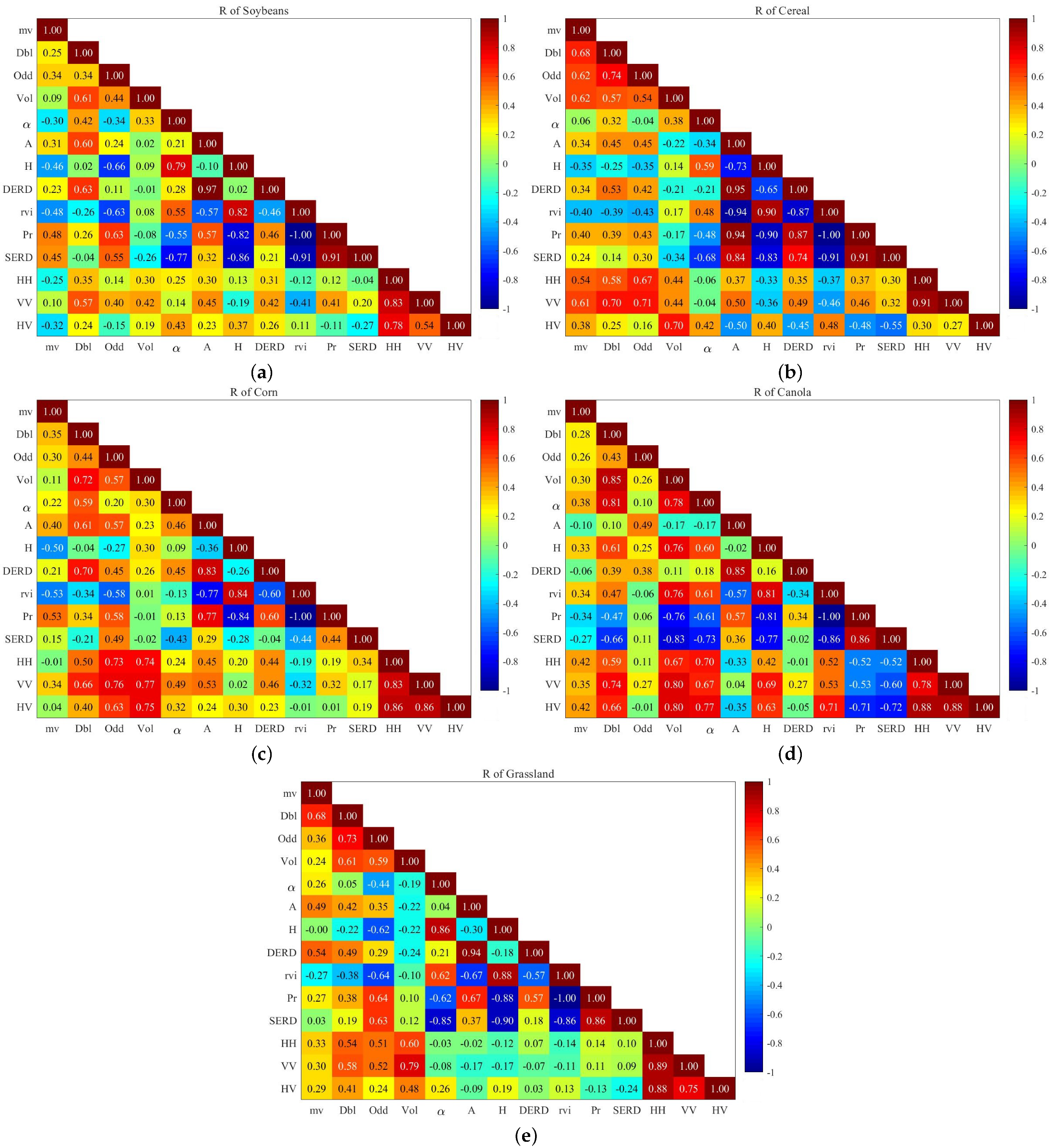
In vegetation-covered regions, soil surface scattering is often coupled with vegetation scattering, complicating the relationship between SSM and SAR backscattering coefficients. Figure 2 shows that the backscattering coefficients of most crops are very similar. In addition, the backscattering coefficient is insensitive to the variation of in situ SSM. This is because parameters such as the moisture content and height of the crops differ at different data acquisition times. The contribution of these crop parameters and SSM to the backscattering coefficients is coupled, so it is difficult to estimate the SSM based on the backscattering coefficients alone. Polarimetric decomposition can explain the scattering mechanism and separate the scattering of vegetation from the surface, which has excellent potential for SSM estimation of polarimetric data. The correlation coefficient matrices of in situ SSM and some commonly used polarimetric decomposition parameters under different crops are given in Figure 4. As shown in Figure 4, the correlation between the surface scattering component and in situ SSM is not the highest under all crops, so estimating the SSM in the experimental area with the first-order Bragg surface scatter results in more significant errors. The correlation between double-bounce scattering and in situ SSM is higher in corn, grassland, and cereal-covered areas, suggesting that dihedral angle scattering exists in these vegetation-covered areas. Typically, volume scattering is ignored in the estimation of SSM, but Figure 4 suggests a significant correlation between volume scattering and in situ SSM in areas covered by canola and cereal. In addition, , A, H, , , , and all showed a relatively high correlation between in situ SSM under different crop covers.
Therefore, estimating SSM using only one or a few polarimetric decomposition parameters may result in significant uncertainties. A scheme that can take into account various polarimetric parameters is essential to estimate SSM accurately. QRF is a method that considers all polarimetric parameters and quantifies the importance of polarimetric parameters in SSM estimation.
4.2. SSM Estimation of Different Crop Coverage Areas
After analyzing the correlation between polarimetric parameters and SSM under different crops, QRF is used to estimate SSM, which is then compared with the performance of CQR. For each crop, four-fifths of the data are randomly selected to train the model and the remaining one-fifth to validate the model. The training and validation datasets of CQR are consistent with the QRF. The number of leaf nodes and decision trees of the random forest is determined by the mean square error between the in situ and the estimated SSM values of the training data. Figure 5 compares the in situ SSM and the SSM estimated by the two methods in the validation dataset. In the figure, the expression of the error is: , where represents the estimated SSM and represents the in situ SSM. As seen in the figures, all scatter points are distributed on both sides of the 1:1 straight line, indicating that both methods can potentially estimate SSM in these crops-covered areas. The histograms show that most of the estimated errors of SSM are between −0.1 cm/cm and 0.1 cm/cm, which shows that both estimation methods are robust. From Figure 5a,b, it can be concluded that the SSM values estimated by QRF in the area covered by soybean and cereal are significantly closer to the measured values than those estimated by CQR. Meanwhile, Figure 5b,d also illustrate that the error range of QRF estimation is smaller than that of CQR. These indicate that QRF is more advantageous than CQR for SSM estimation of soybean and cereal in the dataset used in this study. It is difficult to distinguish which method is more beneficial in the figures from the other three crops.
The evaluation parameters of the two methods for estimating SSM in areas covered by different crops are given in Table 4 to compare the two methods quantitatively. Table 4 suggests that the MRE estimated by the two methods is approximate in the area covered by five crops, which indicates that the estimated deviations of the two methods are similar. The use of QRF reduced the SSM estimated RMSE in the areas covered by crops soybean, cereal, and corn with 0.021 cm/cm, 0.033 cm/cm, and 0.006 cm/cm, respectively. RMSEs estimated by the two methods in canola and grassland-covered areas are not significantly different. Consistent with RMSE, the R and KEG parameters of QRF are considerably better than those of CQR in soybean, cereal, and corn-covered areas. In the canola-covered area, the R of QRF is higher than CQR by 0.025, but the KEG is 0.085 lower than CQR. Both R and KEG of CQR are better than those of QRF in the grassland areas. Combining Table 2 and Table 4, we have found that with the increase in the number of field measurements, the SSM estimated by QRF gradually changes from slightly worse than CQR to significantly better than CQR. This phenomenon may be because the random forest has little data to train each decision tree when the measurement data is small. The estimated value of SSM is not as accurate as that of the traditional copula method. Compared with the RMSE and R evaluated by Wang, H. et al. [33] with the same dataset in 2017 and 2019, the two methods of estimating SSM in this study have obtained more accurate results.
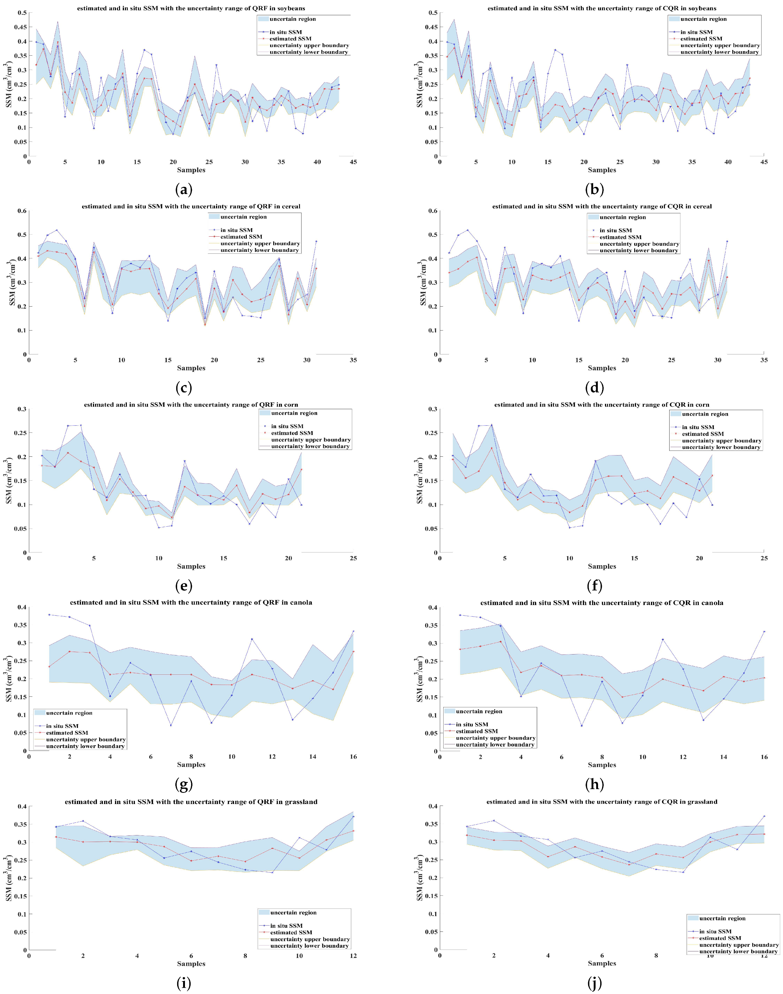
The SSM values for each in situ measurement and estimate accompanying the uncertainty range in the validation data set are given in Figure 6. The figures display that the dynamic range of the in situ SSM is more extensive than that of the estimated SSM for all the crop-covered areas. Most of the in situ SSM falls within the estimated uncertainty interval, and in situ SSM outside the uncertainty interval are usually peaks and valleys. These analyses illustrate the difficulty of both methods in predicting SSM for peaks and valleys, which is consistent with the conclusion of Nguyen, H.H. et al. in 2021 [30]. The evaluation parameters for the estimated uncertainty intervals are the RDA in Table 4, from which it is evident that moderate to good results are obtained for both methods in all crop-covered areas. Figure 6a–f suggest that QRF is more potential than CQR in capturing the peaks and valleys of in situ SSM in areas covered by three crops: soybean, cereal, and corn. While in the areas covered by the other two crops, no significant difference is found between the two methods.
4.3. Parameter Importance Assessment
In addition to the uncertainty interval of the estimate, the QRF can also evaluate the importance of the input parameters to the estimated result, making it possible to understand the contribution of different polarimetric decomposition parameters and backscattering coefficients to the SSM estimate. Figure 7 shows the ordered importance of polarimetric parameters and backscattering coefficients in soybean, cereal, canola, and grassland areas. These phenomena indicate that even for L-band SAR data, the scattering is strongly influenced by the vegetation structure, which is consistent with the conclusions of the correlation analysis in Figure 4. Wang H. et al. [52] found that the importance of different polarimetric parameters for estimating the phenology of varying vegetation varies greatly, which also confirms the influence of vegetation structure on polarimetric parameters.
For soybean, the backscattering coefficient of HH polarization is most important for SSM estimation. Volume scattering is most important in SSM estimates for cereal-covered areas and cannot be ignored in grassland and soybean-covered areas. The H parameter is the most important in SSM estimates for corn-covered areas, only to HH backscattering coefficient and Pr in soybean-covered areas. Surface scattering, often used to estimate SSM, occupies the second most important position in corn and canola-covered regions. The most advantageous parameter for SSM estimation in areas covered by grassland is the double-bounce scattering component, which has the potential to estimate SSM in all crop-covered areas except canola. In addition, in canola and grassland, the importance of some parameters became negative, which indicated that the participation of these parameters in SSM estimation would reduce the estimation accuracy. The main reason for the negative importance is that the out-of-bag importance evaluation method used by random forest is biased [67,68]. When predictors are correlated, randomly shuffled variables are replaced by correlated variables. The analysis of the importance of different parameters helps to select more relevant prediction parameters, simplifying the model in the subsequent development of the SSM estimation model. In summary, these parameters, which are essential in different crops, may have more significant advantages in subsequent SSM estimation studies.
5. Discussion
The backscattering process in vegetation-covered areas is complex, so single-polarized SAR requires optical remote sensing or measured vegetation information to model vegetation scattering. Polarimetric SAR data can separate the contributions of vegetation scattering and surface scattering with the help of polarimetric decomposition, which makes it possible to estimate the SSM of vegetation-covered areas with SAR data alone. From the correlation coefficients in Figure 4 and the importance assessment in Figure 7, it can be found that volume scattering is not negligible in all crops, which also appeared in the study by Bai X. et al. [48]. This phenomenon may be because vegetation water content and growth status are related to SSM, which is the theoretical basis of some optical remote sensing estimation methods for SSM [7]. Meanwhile, the most significant disadvantage of model-based polarimetric decomposition is that the coherence matrix or covariance matrix is decomposed into definite scattering components, regardless of whether these components exist in the actual scattering. This disadvantage results in a weaker correlation between surface scattering and in situ SSM than volume or double-bounce scattering.
The parameters of the eigenvalue-based polarimetric decomposition can explain the scattering mechanism, which is used as auxiliary data in the SSM estimation. As in the study by Hajnsek, I. et al. [39], the H parameter and parameter are highly correlated with the SSM of the bare surface, and the A parameter is highly correlated with the surface roughness. The study by Baghdadi, N. et al. [45] also showed that the parameter has higher sensitivity in areas with high SSM, which can be used to correct the problem of SSM underestimation. Bai X. et al. [48] also found that the best results can be obtained when all the selected decomposition parameters are used for SSM estimation. From the error histogram in Figure 5, the error of the QRF estimate is about the same on both sides of 0, except for the cereal-covered areas. There is an underestimation of SSM in the cereal-covered areas, which may be caused by the inability of the model to capture the high SSM accurately. In other vegetation cover areas, there is no apparent overestimation or underestimation.
Comparing the evaluation parameters in Table 4 shows that the highest R and KEG are obtained for the QRF estimates in the areas covered by cereal. This result may be due to the small spacing between grains, which can be approximated as uniform coverage on the surface, so the correlation between backscattering and SSM is less affected by vegetation, as illustrated by the correlation coefficients in Figure 4. Grasslands, which have the same small plant spacing as cereals, are estimated with low bias by both methods. The possible reasons for the small R of the grassland are that the amount of data is too small to train an optimal model, or the variation range of in situ SSM in the validation dataset is too small. Despite the large spacing between corn plants, the density of corn is essentially the same in different fields in the experimental area, so a high R is also obtained. Unlike cereal, grassland and corn, there are differences in planting density in the areas covered by soybeans, with some producers using double seeding rows [54]. Figure 5a,b illustrate that the estimated SSM for the area covered by soybean has more points with more significant errors. This suggests that differences in planting methods and vegetation biomass impact SSM estimate significantly. Canola is also grown differently; the biomass varies more among fields than soybeans.
In addition to vegetation species and biomass, surface roughness is an important factor affecting SSM estimation. SMAPVEX12 measured the surface roughness of each field. Table 5 presents the statistical information of the surface roughness measured by SMAPVEX12 in areas covered by different vegetation to analyze the relationship between SSM estimation and surface roughness. Two parameters mainly measure surface roughness: the surface root mean square height (s) and the correlation length (l). Table 5 illustrates that the surface roughness varies considerably in different fields. Typically, for wavelength , the roughness is scaled to and , where . Table 5 shows that the range of and are 0.09 0.60 and 0.66 6.73, which indicates that some fields do not satisfy the surface scattering model of Freeman-Durden decomposition [39]. This analysis of Table 5 explains the low importance of surface scattering in SSM estimation from a roughness perspective. A comparison of the average roughness and the accuracy of SSM estimation for different crops suggests no significant relationship between them. This phenomenon indicates that the effect of vegetation on SSM estimation is more significant than the effect of roughness.
Figure 6 suggests that the method proposed in this study has a significant error in the capture of peaks and valleys, which has also appeared in the study of Nguyen, H.H. et al. [30]. Especially in the canola-covered areas, (g) and (h) of Figure 6 show that both methods are ineffective in capturing peaks and valleys, which may also be related to the differences in biomass and the structure. However, these peaks and valleys have important implications for predicting drought and flood. Typically, the peak in the time series occurs after rain or irrigation, and the valley appears long after rainfall. Therefore, heavy precipitation may have a greater impact on the accuracy of the method proposed in this experiment. Many scholars have explored the correlation between SSM and precipitation, and these studies show that SSM is an essential parameter for precipitation prediction, while precipitation affects SSM [69,70,71]. The effect of precipitation in SSM estimation is not considered because precipitation amount and time are not recorded in the data of this experiment. In the follow-up research, factors such as precipitation and the time difference between measurement and precipitation will be considered to improve the estimation accuracy of peak and valley values.
6. Conclusions
This study investigates SSM estimation methods for areas covered by different crops using L-band polarimetric parameters. QRF and CQR are used to estimate SSM from polarimetric parameters. The polarimetric parameters used in the study include the backscattering coefficients of the three polarizations and the parameters obtained from the model-based decomposition and the eigenvalue decomposition. The estimation results show that the QRF algorithm obtains a more accurate estimate with a minimum R of 0.665 and a maximum RMSE of 0.079 cm/cm. The reasonable and satisfactory results of this experiment indicate the potential of spaceborne polarimetric L-band SAR for SSM estimation in vegetation-covered areas, which means that SSM can be monitored periodically. However, there are still some problems. The algorithm proposed in this paper has unavoidable inaccuracy in capturing the peaks and valleys of SSM. In the subsequent study, the influence of precipitation and precipitation time will be considered in the algorithm of SSM estimation further to improve the capture ability of peak and valley values.
Author Contributions
Conceptualization, L.Z. and R.W.; Data curation, L.Z.; Formal analysis, R.W.; Methodology, L.Z.; Project administration, X.L.; Software, L.Z.; Supervision, X.L.; Visualization, L.Z.; Writing—original draft, L.Z.; Writing—review & editing, X.L. and R.W. All authors have read and agreed to the published version of the manuscript.
Funding
This research was funded by the LuTan-1 L-Band Spaceborne Bistatic SAR Data Processing Program, grant number E0H2080702.
Data Availability Statement
The data that support the findings of this study are available from the corresponding author upon reasonable request.
Acknowledgments
The authors would like to thank the entire team at SMAPVEX12 for the experimental success and generous public datasets. We also thank the anonymous reviewers for helping us revise and improve our manuscript.
Conflicts of Interest
The authors declare no conflict of interest.
References
- Moran, M.S.; Inoue, Y.; Barnes, E.M. Opportunities and limitations for image-based remote sensing in precision crop management. Remote Sens. Environ. 1997, 61, 319–346. [Google Scholar] [CrossRef]
- El Hajj, M.; Baghdadi, N.; Zribi, M.; Belaud, G.; Cheviron, B.; Courault, D.; Charron, F. Soil moisture retrieval over irrigated grassland using X-band SAR data. Remote Sens. Environ. 2016, 176, 202–218. [Google Scholar] [CrossRef]
- Zhao, H.; Di, L.; Sun, Z.; Hao, P.; Yu, E.; Zhang, C.; Lin, L. Impacts of Soil Moisture on Crop Health: A Remote Sensing Perspective. In Proceedings of the 2021 9th International Conference on Agro-Geoinformatics (Agro-Geoinformatics), Shenzhen, China, 26–29 July 2021; pp. 1–4. [Google Scholar]
- Norbiato, D.; Borga, M.; Degli Esposti, S.; Gaume, E.; Anquetin, S. Flash flood warning based on rainfall thresholds and soil moisture conditions: An assessment for gauged and ungauged basins. J. Hydrol. 2008, 362, 274–290. [Google Scholar] [CrossRef]
- Abowarda, A.S.; Bai, L.; Zhang, C.; Long, D.; Li, X.; Huang, Q.; Sun, Z. Generating surface soil moisture at 30 m spatial resolution using both data fusion and machine learning toward better water resources management at the field scale. Remote Sens. Environ. 2021, 255, 112301. [Google Scholar] [CrossRef]
- Peng, J.; Albergel, C.; Balenzano, A.; Brocca, L.; Cartus, O.; Cosh, M.H.; Crow, W.T.; Dabrowska-Zielinska, K.; Dadson, S.; Davidson, M.W.; et al. A roadmap for high-resolution satellite soil moisture applications–confronting product characteristics with user requirements. Remote Sens. Environ. 2021, 252, 112162. [Google Scholar] [CrossRef]
- Babaeian, E.; Sadeghi, M.; Franz, T.E.; Jones, S.; Tuller, M. Mapping soil moisture with the OPtical TRApezoid Model (OPTRAM) based on long-term MODIS observations. Remote Sens. Environ. 2018, 211, 425–440. [Google Scholar] [CrossRef]
- Peters, J.; De Baets, B.; De Clercq, E.M.; Ducheyne, E.; Verhoest, N.E. The potential of multitemporal Aqua and Terra MODIS apparent thermal inertia as a soil moisture indicator. Int. J. Appl. Earth Obs. Geoinf. 2011, 13, 934–941. [Google Scholar]
- Wang, H.; Magagi, R.; Goita, K.; Wang, K. Soil moisture retrievals using ALOS2-ScanSAR and MODIS synergy over Tibetan Plateau. Remote Sens. Environ. 2020, 251, 112100. [Google Scholar] [CrossRef]
- Dorigo, W.; Wagner, W.; Albergel, C.; Albrecht, F.; Balsamo, G.; Brocca, L.; Chung, D.; Ertl, M.; Forkel, M.; Gruber, A.; et al. ESA CCI Soil Moisture for improved Earth system understanding: State-of-the art and future directions. Remote Sens. Environ. 2017, 203, 185–215. [Google Scholar] [CrossRef]
- Shi, H.; Zhao, L.; Yang, J.; Lopez-Sanchez, J.M.; Zhao, J.; Sun, W.; Shi, L.; Li, P. Soil moisture retrieval over agricultural fields from L-band multi-incidence and multitemporal PolSAR observations using polarimetric decomposition techniques. Remote Sens. Environ. 2021, 261, 112485. [Google Scholar] [CrossRef]
- Kerr, Y.H.; Waldteufel, P.; Wigneron, J.P.; Martinuzzi, J.M.; Font, J.; Berger, M. Soil Moisture Retrieval from Space: The Soil Moisture and Ocean Salinity (SMOS) Mission. IEEE Trans. Geosci. Remote Sens. 2001, 39, 1729–1735. [Google Scholar] [CrossRef]
- Entekhabi, D.; Njoku, E.G.; O’Neill, P.E.; Kellogg, K.H.; Crow, W.T.; Edelstein, W.N.; Entin, J.K.; Goodman, S.D.; Jackson, T.J.; Johnson, J.; et al. The soil moisture active passive (SMAP) mission. Proc. IEEE 2010, 98, 704–716. [Google Scholar] [CrossRef]
- Chen, K.S.; Wu, T.D.; Tsay, M.K.; Fung, A.K. Note on the multiple scattering in an IEM model. IEEE Trans. Geosci. Remote Sens. 2000, 38, 249–256. [Google Scholar] [CrossRef]
- Chen, K.S.; Wu, T.D.; Tsang, L.; Qin, L.; Fung, A.K. Emission of rough surfaces calculated by the integral equation method with comparison to three-dimensional moment method simulations. IEEE Trans. Geosci. Remote Sens. 2003, 41, 90–101. [Google Scholar] [CrossRef]
- Fung, A.K.; Chen, K.S. An Update on the IEM Surface Backscattering Model. IEEE Geosci. Remote Sens. Lett. 2004, 1, 75–77. [Google Scholar] [CrossRef]
- Dubois, P.C.; Van Zyl, J.; Engman, T. Measuring soil moisture with imaging radars. IEEE Trans. Geosci. Remote Sens. 2002, 33, 915–926. [Google Scholar] [CrossRef]
- Nicolas, B.; Mohammad, C.; Mehrez, Z.; Mohammad, H.; Simonetta, P.; Niko, V.; Hans, L.; Frederic, B.; Francesco, M. A new empirical model for radar scattering from bare soil surfaces. Remote Sens. 2016, 8, 920. [Google Scholar] [CrossRef]
- Shi, J.; Wang, J.; Hsu, A.Y.; O’Neill, P.E.; Engman, E.T. Estimation of bare soil moisture and surface roughness parameters using L-band SAR image data. IEEE Trans. Geosci. Remote Sens. 1997, 35, 1254–1266. [Google Scholar]
- Oh, Y.; Sarabandi, K.; Ulaby, F.T. Semi-empirical model of the ensemble-averaged differential Mueller matrix for microwave backscattering from bare soil surfaces. IEEE Trans. Geosci. Remote Sens. 2002, 40, 1348–1355. [Google Scholar] [CrossRef]
- Zhu, L.; Walker, J.P.; Ye, N.; Rüdiger, C. Roughness and vegetation change detection: A pre-processing for soil moisture retrieval from multi-temporal SAR imagery. Remote Sens. Environ. 2019, 225, 93–106. [Google Scholar] [CrossRef]
- Attema, E.P.W.; Ulaby, F.T. Vegetation modeled as a water cloud. Radio Sci. 1978, 13, 357–364. [Google Scholar] [CrossRef]
- Ulaby, F.T.; Sarabandi, K.; Mcdonald, K.; Whitt, M.; Dobson, M.C. Michigan microwave canopy scattering model. Int. J. Remote Sens. 1990, 11, 1223–1253. [Google Scholar] [CrossRef]
- Baghdadi, N.N.; El Hajj, M.; Zribi, M.; Fayad, I. Coupling SAR C-band and optical data for soil moisture and leaf area index retrieval over irrigated grasslands. IEEE J. Sel. Top. Appl. Earth Obs. Remote Sens. 2015, 9, 1229–1243. [Google Scholar] [CrossRef]
- Bai, X.; He, B.; Li, X.; Zeng, J.; Wang, X.; Wang, Z.; Zeng, Y.; Su, Z. First assessment of Sentinel-1A data for surface soil moisture estimations using a coupled water cloud model and advanced integral equation model over the Tibetan Plateau. Remote Sens. 2017, 9, 714. [Google Scholar] [CrossRef]
- Pathe, C.; Wagner, W.; Sabel, D.; Doubkova, M.; Basara, J.B. Using ENVISAT ASAR global mode data for surface soil moisture retrieval over Oklahoma, USA. IEEE Trans. Geosci. Remote Sens. 2009, 47, 468–480. [Google Scholar] [CrossRef]
- Kim, Y.; van Zyl, J.J. A time-series approach to estimate soil moisture using polarimetric radar data. IEEE Trans. Geosci. Remote Sens. 2009, 47, 2519–2527. [Google Scholar]
- Pal, M.; Maity, R.; Suman, M.; Das, S.K.; Patel, P.; Srivastava, H.S. Satellite-based probabilistic assessment of soil moisture using C-band quad-polarized RISAT1 data. IEEE Trans. Geosci. Remote Sens. 2016, 55, 1351–1362. [Google Scholar] [CrossRef]
- Ma, C.; Li, X.; Notarnicola, C.; Wang, S.; Wang, W. Uncertainty quantification of soil moisture estimations based on a Bayesian probabilistic inversion. IEEE Trans. Geosci. Remote Sens. 2017, 55, 3194–3207. [Google Scholar] [CrossRef]
- Nguyen, H.H.; Cho, S.; Jeong, J.; Choi, M. A D-vine copula quantile regression approach for soil moisture retrieval from dual polarimetric SAR Sentinel-1 over vegetated terrains. Remote Sens. Environ. 2021, 255, 112283. [Google Scholar] [CrossRef]
- Hajnsek, I.; Jagdhuber, T.; Schon, H.; Papathanassiou, K.P. Potential of estimating soil moisture under vegetation cover by means of PolSAR. IEEE Trans. Geosci. Remote Sens. 2009, 47, 442–454. [Google Scholar] [CrossRef]
- Huang, X.; Wang, J.; Shang, J. An adaptive two-component model-based decomposition on soil moisture estimation for C-band RADARSAT-2 imagery over wheat fields at early growing stages. IEEE Geosci. Remote Sens. Lett. 2016, 13, 414–418. [Google Scholar] [CrossRef]
- Wang, H.; Magagi, R.; Goita, K. Comparison of different polarimetric decompositions for soil moisture retrieval over vegetation covered agricultural area. Remote Sens. Environ. 2017, 199, 120–136. [Google Scholar] [CrossRef]
- Wang, H.; Magagi, R.; Goïta, K. Potential of a two-component polarimetric decomposition at C-band for soil moisture retrieval over agricultural fields. Remote Sens. Environ. 2018, 217, 38–51. [Google Scholar] [CrossRef]
- Notarnicola, C.; Angiulli, M.; Posa, F. Soil moisture retrieval from remotely sensed data: Neural network approach versus Bayesian method. IEEE Trans. Geosci. Remote Sens. 2008, 46, 547–557. [Google Scholar] [CrossRef]
- Paloscia, S.; Pettinato, S.; Santi, E.; Notarnicola, C.; Pasolli, L.; Reppucci, A. Soil moisture mapping using Sentinel-1 images: Algorithm and preliminary validation. Remote Sens. Environ. 2013, 134, 234–248. [Google Scholar] [CrossRef]
- Santi, E.; Paloscia, S.; Pettinato, S.; Fontanelli, G. Application of artificial neural networks for the soil moisture retrieval from active and passive microwave spaceborne sensors. Int. J. Appl. Earth Obs. Geoinf. 2016, 48, 61–73. [Google Scholar] [CrossRef]
- Kumar, P.; Prasad, R.; Choudhary, A.; Gupta, D.; Mishra, V.; Vishwakarma, A.; Singh, A.; Srivastava, P. Comprehensive evaluation of soil moisture retrieval models under different crop cover types using C-band synthetic aperture radar data. Geocarto Int. 2019, 34, 1022–1041. [Google Scholar] [CrossRef]
- Hajnsek, I.; Pottier, E.; Cloude, S.R. Inversion of surface parameters from polarimetric SAR. IEEE Trans. Geosci. Remote Sens. 2003, 41, 727–744. [Google Scholar] [CrossRef]
- He, L.; Panciera, R.; Tanase, M.A.; Walker, J.P.; Qin, Q. Soil moisture retrieval in agricultural fields using adaptive model-based polarimetric decomposition of SAR data. IEEE Trans. Geosci. Remote Sens. 2016, 54, 4445–4460. [Google Scholar] [CrossRef]
- Jagdhuber, T.; Hajnsek, I.; Papathanassiou, K.P. An iterative generalized hybrid decomposition for soil moisture retrieval under vegetation cover using fully polarimetric SAR. IEEE J. Sel. Top. Appl. Earth Obs. Remote Sens. 2014, 8, 3911–3922. [Google Scholar] [CrossRef]
- Ponnurangam, G.G.; Jagdhuber, T.; Hajnsek, I.; Rao, Y. Soil moisture estimation using hybrid polarimetric SAR data of RISAT-1. IEEE Trans. Geosci. Remote Sens. 2015, 54, 2033–2049. [Google Scholar] [CrossRef]
- Wang, H.; Magagi, R.; Goita, K.; Jagdhuber, T. Refining a polarimetric decomposition of multi-angular UAVSAR time series for soil moisture retrieval over low and high vegetated agricultural fields. IEEE J. Sel. Top. Appl. Earth Obs. Remote Sens. 2019, 12, 1431–1450. [Google Scholar] [CrossRef]
- Gururaj, P.; Umesh, P.; Shetty, A. Assessment of surface soil moisture from ALOS PALSAR-2 in small-scale maize fields using polarimetric decomposition technique. Acta Geophys. 2021, 69, 579–588. [Google Scholar] [CrossRef]
- Baghdadi, N.; Cresson, R.; Pottier, E.; Aubert, M.; Mehrez, M.; Jacome, A.; Benabdallah, S. A potential use for the C-band polarimetric SAR parameters to characterize the soil surface over bare agriculture fields. IEEE Trans. Geosci. Remote Sens. 2012, 50, 3844–3858. [Google Scholar] [CrossRef]
- Bourgeau-Chavez, L.L.; Leblon, B.; Charbonneau, F.; Buckley, J.R. Evaluation of polarimetric Radarsat-2 SAR data for development of soil moisture retrieval algorithms over a chronosequence of black spruce boreal forests. Remote Sens. Environ. 2013, 132, 71–85. [Google Scholar] [CrossRef]
- Pasolli, L.; Notarnicola, C.; Bruzzone, L.; Bertoldi, G.; Chiesa, S.D.; Niedrist, G.; Tappeiner, U.; Zebisch, M. Polarimetric RADARSAT-2 imagery for soil moisture retrieval in alpine areas. Can. J. Remote Sens. 2011, 37, 535–547. [Google Scholar] [CrossRef]
- Bai, X.; He, B.; Xu, D. Potential use of radarsat-2 polarimetric parameters for estimating soil moisture in prairie areas. In Proceedings of the 2016 IEEE International Geoscience and Remote Sensing Symposium (IGARSS), Beijing, China, 10–15 July 2016; pp. 3043–3046. [Google Scholar]
- Zhang, X.; Chen, B.; Zhao, H.; Fan, H.; Zhu, D. Soil moisture retrieval over a semiarid area by means of PCA dimensionality reduction. Can. J. Remote Sens. 2016, 42, 136–144. [Google Scholar] [CrossRef]
- Hariharan, S.; Mandal, D.; Tirodkar, S.; Kumar, V.; Bhattacharya, A.; Lopez-Sanchez, J.M. A novel phenology based feature subset selection technique using random forest for multitemporal PolSAR crop classification. IEEE J. Sel. Top. Appl. Earth Obs. Remote Sens. 2018, 11, 4244–4258. [Google Scholar] [CrossRef]
- Kumar, P.; Prasad, R.; Gupta, D.; Mishra, V.; Vishwakarma, A.; Yadav, V.; Bala, R.; Choudhary, A.; Avtar, R. Estimation of winter wheat crop growth parameters using time series Sentinel-1A SAR data. Geocarto Int. 2018, 33, 942–956. [Google Scholar] [CrossRef]
- Wang, H.; Magagi, R.; Goïta, K.; Trudel, M.; McNairn, H.; Powers, J. Crop phenology retrieval via polarimetric SAR decomposition and Random Forest algorithm. Remote Sens. Environ. 2019, 231, 111234. [Google Scholar] [CrossRef]
- Yadav, V.P.; Prasad, R.; Bala, R.; Vishwakarma, A.K. An improved inversion algorithm for spatio-temporal retrieval of soil moisture through modified water cloud model using C-band Sentinel-1A SAR data. Comput. Electron. Agric. 2020, 173, 105447. [Google Scholar] [CrossRef]
- McNairn, H.; Jackson, T.J.; Wiseman, G.; Belair, S.; Berg, A.; Bullock, P.; Colliander, A.; Cosh, M.H.; Kim, S.B.; Magagi, R.; et al. The soil moisture active passive validation experiment 2012 (SMAPVEX12): Prelaunch calibration and validation of the SMAP soil moisture algorithms. IEEE Trans. Geosci. Remote Sens. 2014, 53, 2784–2801. [Google Scholar] [CrossRef]
- McNairn, H.; Powers, J.; Wiseman, G. SMAPVEX12 Land Cover Classification Map; NASA DAAC at the National Snow and Ice Data Center: Boulder, CO, USA, 2014.
- SMAP Validation Experiment 2012. Experimental Plan. Available online: https://nsidc.org/sites/nsidc.org/files/technical-references/SMAPVEX12_Experiment_Plan.pdf (accessed on 5 May 2022).
- SMAP Validation Experiment 2012. SMAPVEX12 Database Report. Available online: https://nsidc.org/sites/nsidc.org/files/technical-references/SMAPVEX12-database-report-final.pdf (accessed on 5 May 2022).
- Dataset: UAVSAR, NASA. 2012. Retrieved from ASF DAAC 12 December 2021. Available online: https://search.asf.alaska.edu/ (accessed on 21 August 2022).
- Wiseman, G.; Bullock, P.; Berg, A. SMAPVEX12 Probe-Based In Situ Soil Moisture Data for Agricultural Area; NASA National Snow and Ice Data Center Distributed Active Archive Center: Boulder, CO, USA, 2014.
- Freeman, A.; Durden, S.L. A three-component scattering model for polarimetric SAR data. IEEE Trans. Geosci. Remote Sens. 1998, 36, 963–973. [Google Scholar] [CrossRef] [Green Version]
- Lee, J.S.; Pottier, E. Polarimetric Radar Imaging: From Basics to Applications; CRC Press: Boca Raton, FL, USA, 2017. [Google Scholar]
- Cloude, S.R.; Pottier, E. An entropy based classification scheme for land applications of polarimetric SAR. IEEE Trans. Geosci. Remote Sens. 1997, 35, 68–78. [Google Scholar] [CrossRef]
- Mladenova, I.E.; Jackson, T.J.; Bindlish, R.; Hensley, S. Incidence angle normalization of radar backscatter data. IEEE Trans. Geosci. Remote Sens. 2012, 51, 1791–1804. [Google Scholar] [CrossRef]
- Meinshausen, N.; Ridgeway, G. Quantile regression forests. J. Mach. Learn. Res. 2006, 7, 983–999. [Google Scholar]
- Nelsen, R.B. An Introduction to Copulas; Springer Science & Business Media: Berlin/Heidelberg, Germany, 2007. [Google Scholar]
- Bair, E.; Hastie, T.; Paul, D.; Tibshirani, R. Prediction by supervised principal components. J. Am. Stat. Assoc. 2006, 101, 119–137. [Google Scholar] [CrossRef]
- Janitza, S.; Strobl, C.; Boulesteix, A.L. An AUC-based permutation variable importance measure for random forests. BMC Bioinform. 2013, 14, 1–11. [Google Scholar] [CrossRef]
- Strobl, C.; Boulesteix, A.L.; Zeileis, A.; Hothorn, T. Bias in random forest variable importance measures: Illustrations, sources and a solution. BMC Bioinform. 2007, 8, 1–21. [Google Scholar] [CrossRef]
- Koster, R.D.; Dirmeyer, P.A.; Guo, Z.; Bonan, G.; Chan, E.; Cox, P.; Gordon, C.; Kanae, S.; Kowalczyk, E.; Lawrence, D.; et al. Regions of strong coupling between soil moisture and precipitation. Science 2004, 305, 1138–1140. [Google Scholar] [CrossRef]
- Wu, W.; Geller, M.A.; Dickinson, R.E. The response of soil moisture to long-term variability of precipitation. J. Hydrometeorol. 2002, 3, 604–613. [Google Scholar] [CrossRef]
- Wagner, W.; Scipal, K.; Pathe, C.; Gerten, D.; Lucht, W.; Rudolf, B. Evaluation of the agreement between the first global remotely sensed soil moisture data with model and precipitation data. J. Geophys. Res. Atmos. 2003, 108. [Google Scholar] [CrossRef]
Figure 1.
The map of the geographical location of the experimental area, vegetation classification map, coverage of the four flights, and in situ SSM measurement points.
Figure 1.
The map of the geographical location of the experimental area, vegetation classification map, coverage of the four flights, and in situ SSM measurement points.

Figure 2.
Sensitivity analysis between SAR backscattering coefficients and in situ SSM under different crops. (a) HH polarization and in situ SSM; (b) VV polarization and in situ SSM; (c) HV polarization and in situ SSM.
Figure 2.
Sensitivity analysis between SAR backscattering coefficients and in situ SSM under different crops. (a) HH polarization and in situ SSM; (b) VV polarization and in situ SSM; (c) HV polarization and in situ SSM.

Figure 3.
Flowchart of the algorithm for estimating soil moisture (SSM) from L-band UAVSAR data combining polarimetric decomposition and quantile regression forests (QRF).
Figure 3.
Flowchart of the algorithm for estimating soil moisture (SSM) from L-band UAVSAR data combining polarimetric decomposition and quantile regression forests (QRF).

Figure 4.
Correlation coefficient matrices of in situ SSM and some commonly used polarimetric decomposition parameters under different crop coverage. (a) correlation coefficient matrix of soybeans; (b) correlation coefficient matrix of cereal; (c) correlation coefficient matrix of corn; (d) correlation coefficient matrix of canola; (e) correlation coefficient matrix of grassland.

Figure 5.
Scatter plot and error histogram of the estimated and in situ SSM. (a) Scatter plot of soybeans; (b) Error histogram of soybeans; (c) Scatter plot of cereal; (d) Error histogram of cereal; (e) Scatter plot of corn; (f) Error histogram of corn; (g) Scatter plot of canola; (h) Error histogram of canola; (i) Scatter plot of grassland; (j) Error histogram of grassland.

Figure 6.
Estimated and in situ SSM with the uncertainty intervals. (a) uncertainty intervals of QRF in soybeans; (b) uncertainty intervals of CQR in soybeans; (c) uncertainty intervals of QRF in cereal; (d) uncertainty intervals of CQR in cereal; (e) uncertainty intervals of QRF in corn; (f) uncertainty intervals of CQR in corn; (g) uncertainty intervals of QRF in canola; (h) uncertainty intervals of CQR in canola; (i) uncertainty intervals of QRF in grassland; (j) uncertainty intervals of CQR in grassland.

Figure 7.
Importance of the polarimetric parameters and backscattering coefficients for estimated SSM. (a) Importance of the parameters for estimated SSM in soybeans; (b) Importance of the parameters for estimated SSM in cereal; (c) Importance of the parameters for estimated SSM in corn; (d) Importance of the parameters for estimated SSM in canola; (e) Importance of the parameters for estimated SSM in grassland.


Table 1.
Slope and correlation coefficients (R) between in situ SSM and backscattering coefficients for different crop coverage areas.
Table 1.
Slope and correlation coefficients (R) between in situ SSM and backscattering coefficients for different crop coverage areas.
| Sensitivity | Polarization | Canola | Corn | Grassland | Soybeans | Cereal |
|---|---|---|---|---|---|---|
| slope | HH | 10.27 | −0.59 | 12.17 | −6.32 | 9.90 |
| VV | 9.18 | 18.61 | 8.50 | 1.90 | 11.94 | |
| HV | 17.78 | 3.22 | 14.82 | −9.85 | 8.83 | |
| R | HH | 0.42 | -0.01 | 0.33 | −0.27 | 0.55 |
| VV | 0.35 | 0.34 | 0.30 | 0.09 | 0.59 | |
| HV | 0.42 | 0.04 | 0.29 | −0.32 | 0.38 |
Table 2.
Statistical parameters for the minimum (MIN), mean (MEAN), maximum (MAX), standard deviation (STD), and the number of measurements (N) of the in situ SSM.
Table 2.
Statistical parameters for the minimum (MIN), mean (MEAN), maximum (MAX), standard deviation (STD), and the number of measurements (N) of the in situ SSM.
| Crop | MIN cm/cm | MEAN cm/cm | MAX cm/cm | STD cm/cm | N |
|---|---|---|---|---|---|
| soybeans | 0.052 | 0.220 | 0.588 | 0.105 | 201 |
| cereal | 0.087 | 0.294 | 0.525 | 0.110 | 150 |
| corn | 0.052 | 0.137 | 0.313 | 0.057 | 102 |
| canola | 0.059 | 0.207 | 0.378 | 0.087 | 76 |
| grassland | 0.159 | 0.296 | 0.538 | 0.071 | 58 |
Table 3.
Statistical parameters for the minimum (MIN), mean (MEAN), maximum (MAX) and standard deviation (STD) of the height of crops.
Table 3.
Statistical parameters for the minimum (MIN), mean (MEAN), maximum (MAX) and standard deviation (STD) of the height of crops.
| Crop | MIN cm | MEAN cm | MAX cm | STD cm |
|---|---|---|---|---|
| soybeans | 7.0 | 26.6 | 75.9 | 17.5 |
| cereal | 33.7 | 74.2 | 113.6 | 17.6 |
| corn | 13.2 | 102.9 | 269.6 | 73.2 |
| canola | 6.5 | 88.2 | 148.2 | 37.4 |
| grassland | 5.9 | 30.5 | 66.1 | 15.9 |
Table 4.
Evaluation parameters of the error between estimated SSM and in situ SSM.
| Crop | Method | MRE | RMSE | R | KGE | RDA |
|---|---|---|---|---|---|---|
| soybeans | QRF | 0.101 | 0.059 | 0.745 | 0.612 | 0.107 |
| CQR | 0.109 | 0.080 | 0.481 | 0.384 | 0.121 | |
| cereal | QRF | 0.002 | 0.053 | 0.905 | 0.732 | 0.012 |
| CQR | −0.003 | 0.086 | 0.710 | 0.491 | 0.004 | |
| corn | QRF | 0.120 | 0.037 | 0.802 | 0.577 | 0.140 |
| CQR | 0.197 | 0.043 | 0.715 | 0.458 | 0.222 | |
| canola | QRF | 0.227 | 0.079 | 0.763 | 0.288 | 0.155 |
| CQR | 0.202 | 0.075 | 0.738 | 0.373 | 0.190 | |
| grassland | QRF | 0.001 | 0.037 | 0.665 | 0.431 | −0.009 |
| CQR | −0.003 | 0.036 | 0.718 | 0.488 | −0.008 |
Table 5.
Statistical parameters for the minimum (MIN), mean (MEAN), maximum (MAX) and standard deviation (STD) of the surface roughness parameters (SRP): surface root mean square height (s) and correlation length (l) (unit: cm).
Table 5.
Statistical parameters for the minimum (MIN), mean (MEAN), maximum (MAX) and standard deviation (STD) of the surface roughness parameters (SRP): surface root mean square height (s) and correlation length (l) (unit: cm).
| Crop | SRP | MIN | MEAN | MAX | STD |
|---|---|---|---|---|---|
| soybeans | s | 0.34 | 0.88 | 1.89 | 0.32 |
| l | 5.50 | 11.88 | 18.5 | 3.58 | |
| cereal | s | 0.44 | 1.14 | 2.26 | 0.40 |
| l | 2.50 | 11.03 | 25.50 | 5.02 | |
| corn | s | 0.60 | 1.27 | 1.89 | 0.44 |
| l | 6.50 | 12.11 | 22.50 | 4.60 | |
| canola | s | 0.69 | 1.22 | 1.71 | 0.34 |
| l | 6.00 | 9.96 | 15.50 | 3.07 | |
| grassland | s | 0.35 | 1.07 | 1.76 | 0.42 |
| l | 6.00 | 14.00 | 22.50 | 6.21 |
Publisher’s Note: MDPI stays neutral with regard to jurisdictional claims in published maps and institutional affiliations. |
© 2022 by the authors. Licensee MDPI, Basel, Switzerland. This article is an open access article distributed under the terms and conditions of the Creative Commons Attribution (CC BY) license (https://creativecommons.org/licenses/by/4.0/).
Share and Cite
MDPI and ACS Style
Zhang, L.; Lv, X.; Wang, R. Soil Moisture Estimation Based on Polarimetric Decomposition and Quantile Regression Forests. Remote Sens. 2022, 14, 4183. https://0-doi-org.brum.beds.ac.uk/10.3390/rs14174183
AMA Style
Zhang L, Lv X, Wang R. Soil Moisture Estimation Based on Polarimetric Decomposition and Quantile Regression Forests. Remote Sensing. 2022; 14(17):4183. https://0-doi-org.brum.beds.ac.uk/10.3390/rs14174183
Chicago/Turabian StyleZhang, Li, Xiaolei Lv, and Rui Wang. 2022. "Soil Moisture Estimation Based on Polarimetric Decomposition and Quantile Regression Forests" Remote Sensing 14, no. 17: 4183. https://0-doi-org.brum.beds.ac.uk/10.3390/rs14174183
Note that from the first issue of 2016, this journal uses article numbers instead of page numbers. See further details here.