
Built-Up Area Extraction from GF-3 SAR Data Based on a Dual-Attention Transformer Model
by
 , , , ,
Tianyang Li
1,2,3 ,
,
Chao Wang
1,2,3,*,
Fan Wu
1,2,3,
Hong Zhang
1,2,3,
Sirui Tian
4,
Qiaoyan Fu
5 and
Lu Xu
1,2,3 1
Key Laboratory of Digital Earth Science, Aerospace Information Research Institute, Chinese Academy of Sciences, Beijing 100094, China
2
International Research Center of Big Data for Sustainable Development Goals, Beijing 100094, China
3
College of Resources and Environment, University of Chinese Academy of Sciences, Beijing 100049, China
4
Department of Electronic Engineering, School of Electronic and Optical Engineering, Nanjing University of Science and Technology, Nanjing 210094, China
5
China Centre for Resource Satellite Data and Application, Beijing 100094, China
*
Author to whom correspondence should be addressed.
Remote Sens. 2022, 14(17), 4182; https://0-doi-org.brum.beds.ac.uk/10.3390/rs14174182
Submission received: 21 May 2022
/
Revised: 20 July 2022
/
Accepted: 18 August 2022
/
Published: 25 August 2022
(This article belongs to the Special Issue SAR in Big Data Era II)
Abstract
:Built-up area (BA) extraction using synthetic aperture radar (SAR) data has emerged as a potential method in urban research. Currently, typical deep-learning-based BA extractors show high false-alarm rates in the layover areas and subsurface bedrock, which ignore the surrounding information and cannot be directly applied to large-scale BA mapping. To solve the above problems, a novel transformer-based BA extraction framework for SAR images is proposed. Inspired by SegFormer, we designed a BA extractor with multi-level dual-attention transformer encoders. First, the hybrid dilated convolution (HDC) patch-embedding module keeps the surrounding information of the input patches. Second, the channel self-attention module is designed for dual-attention transformer encoders and global modeling. The multi-level structure is employed to produce the coarse-to-fine semantic feature map of BAs. About 1100 scenes of Gaofen-3 (GF-3) data and 200 scenes of Sentinel-1 data were used in the experiment. Compared to UNet, PSPNet, and SegFormer, our model achieved an 85.35% mean intersection over union (mIoU) and 94.75% mean average precision (mAP) on the test set. The proposed framework achieved the best results in both mountainous and plain terrains. The experiments using Sentinel-1 shows that the proposed method has a good generalization ability with different SAR data sources. Finally, the BA map of China for 2020 was obtained with an overall accuracy of about 86%, which shows high consistency with the global urban footprint. The above experiments proved the effectiveness and robustness of the proposed framework in large-scale BA mapping.
1. Introduction
Urbanization is a significant trend in global economic and social development. According to United Nations statistics [1,2,3], by 2050, the urban population will increase from 55% to 68%, and more than half of the population will live in cities. The environmental, economic, political, social, and cultural impacts of urbanization are profound [4,5]. Built-up area (BA) is an essential type of land cover for the urbanization indicator. The extraction of BA is beneficial to guide and evaluate the urbanization process. BA is defined as the land surface covered by building structures that are used for the shelter of humans or economic activities. Remote sensing has gradually become an important tool for obtaining information on the extent and change of urban land due to its ability to regularly observe the surface [6,7,8,9,10,11,12,13,14,15,16,17,18,19,20,21,22,23,24,25,26,27,28,29,30,31,32,33,34,35,36,37,38,39,40,41,42,43,44,45,46].
In recent years, many related studies have reported global-scale products in urban areas [6,7,8,9,10] based on remote sensing technology. The European Commission, Joint Research Centre (JRC), and German Aerospace Center (DLR) have made outstanding contributions in the field of global-scale products in urban areas [11,12,13,14,15]. According to relevant literature, due to the rich reflection features of multispectral data [16], most data sources for global urban area mapping are optical remote-sensing image data (such as Landsat, SPOT, and Sentinel-2). For example, the global human settlement layer (GHSL) [17] utilized massive optical data to generate multi-layered global products, including BA grid and settlement model layers [18].
Synthetic aperture radar (SAR) has become one of the critical tools of earth observation for its all-day and all-weather abilities [19,20]. The characteristics of secondary scattering, roof specular reflection, and shadow of buildings show unique light and dark scattering characteristics in SAR images [21,22,23], which provide the basis for extracting. In addition, the polarization information of SAR images is also beneficial for feature extraction [24,25,26,27,28].
There have been many achievements in BA extraction using SAR images based on methods of image processing. In 2010, T. Esch et al. of DLR conducted related research on TerraSAR-X data [29]. The region-growing algorithm based on local speckle dispersion achieved an average classification accuracy of 90.6%. Two years later, the fully automated processing system urban footprint processor (UFP) was proposed for extracting BAs based on an unsupervised classification scheme [30,31]. The UFP system was optimized to eliminate false alarms by adding an automated post-editing module [32,33,34]. Y. Ban [35] et al. improved the result of urban and rural areas based on the spatial index and gray level co-occurrence matrix texture using ENVISAT ASAR data. M. Chini et al. [36] realized the adaptive search for BA threshold using multi-temporal filtering and coherence coefficient of Sentinel-1 SAR data. H. Cao et al. [37] improved the performance of the region-growing algorithm for BA mapping using spatial indicators and texture features.
Recently, many studies have extracted BAs using deep-learning methods [38,39,40,41,42,43,44,45]. Multiscale convolutional neural networks (CNNs) and textual content in fully convolutional network improved the feature-extraction ability [40,41]. Neighboring pixel information was employed in CNN for higher accuracy prediction [42]. Based on the residual convolutional block (ResNet50), J. Li et al. [43] added the normalized difference vegetation index (NDVI) and the modified normalized difference water index (MNDWI) to solve the high rate of false alarms and omission errors. F. Wu et al. [44] established a deep-learning framework for BA extraction based on improved U-Net and Gaofen-3 data to map urban-area products of China, with an overall accuracy of up to 93.45%. Z. Huang et al. [45] proposed a framework that learns both spatial texture information and backscattering patterns of the complex-valued data. With the popularity of transformers, their performance exceeds CNNs in computer vision. The deep-learning methods show great potential in the field of BA extraction.
Although the above literature has obtained outstanding results, the layover areas and subsurface bedrock show similar representations to BAs. There would be a high number of false alarms in such areas using CNNs. The surrounding information of the patches is lost using the transformer. Most existing self-attention modules are designed for capturing the spatial dependency. They are still insufficient in semantic understanding.
To solve the previously mentioned problems of large-scale mapping, this paper proposes a BA extraction framework based on the dual-attention transformer model and Gaofen-3 (GF-3) data [46]. Inspired by Vision Transformer (ViT) [47] and SegFormer [48], the improved hybrid dilated convolution (HDC) patch-embedding module adds spatial information from around the image patches. It provides a larger receptive field and decreases the information-loss using pixels on target surroundings. The two-dimensional multi-head self-attention mechanism and the pyramid structure are used to guarantee the segmentation accuracy of BA. This structure learns the relationship between features globally. In addition, the combined loss function is used to optimize the mIoU. The proposed method lays the foundation for mapping the BAs using Gaofen-3 data. To prove the validity of the model, data with different terrains and sources was used. Finally, with the support of massive SAR data, we mapped built-up areas of China for 2020. Our product was also compared with the global urban footprint (GUF).
2. Methodology
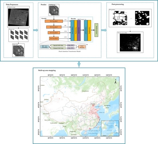
Figure 1 shows the framework for large-scale BA extraction. GF-3 and Sentinel-1 data were acquired for BA mapping. The public data SARBuD [44] and manual annotations were used for the BA dataset. The overall workflow is as follows: (1) image preprocessing: the L1 SAR data is converted to L2 product and cropped into blocks by sliding windows. (2) BA extraction: the dual-attention transformer model is used to predict potential BA areas. (3) Image post-processing: potential BA areas are stitched and mosaicked for the whole map. (4) Accuracy assessment: expert knowledge and Google Earth are used for accuracy assessment.
2.1. Image Preprocessing
Figure 2 shows the process of image preprocessing. The data source used in this paper is the GF-3 L1A product. The steps are mainly geocoding and radiometric correction. The Equations (1) and (2) calculate the backscatter coefficient using the single-look complex (SLC) data [49].
where I and Q are the real and imaginary parts of the image data, respectively, and M is the maximum value before image quantization, located in the QualifyValue field of the metadata product XML file. Likewise, the calibration constant can be found through the CalibrationConst field.
The modified cosine model in Equation (3) [50] is applied for backscattering normalization. Parameter n is the normalization factor, ranging from 2 to 7. is the incidence angle in the scene center. is the local incidence angle referred to the ellipsoid.
The geocoding employs a correction model based on the rational polynomial coefficient (RPC), which can be obtained from the RPC file. The L2 SAR product can be obtained after geocoding and geometric correction using the RPC correction batch program. The image is then stretched between 0 and 255 by many methods, such as a 2% linear stretch. The contrast enhancement is achieved by linear stretching [35,37], which can improve the intensity of building areas with weak dihedral angle scattering [51]. In this way, it can improve the accuracy of BA extraction to a certain extent. On the basis of the L2 SAR product, the image is cropped into sub-image sets for smaller size. A 50% overlap rate was used to obtain these patches. Likewise, after the steps shown in Figure 2, the Sentinel-1 data are processed into the format required by the model.
2.2. Built-Up Areas Extraction Model
The structure of the proposed model, shown in Figure 3, is as follows: (1) In the HDC path-embedding module, dilated convolutions [52] are applied to preserve more spatial information when the image patch was mapped to a linear embedding sequence. (2) Four dual-attention transformer encoders are applied to generate different levels of feature maps from spatial and channel dimensions. (3) The decoder applies two layers of multilayer perceptron (MLP) for fusing high-resolution coarse-grained features and low-resolution fine-grained features. (4) Data augmentation and the combined loss function are employed to improve the generalization ability of the model.
2.2.1. Data Augmentation
Appropriate data augmentation is conducive to improving the performance of the model [53]. In this experiment, a variety of data augmentations, including random cropping, mirror flipping, vertical flipping, and random distortion, were selected to improve the generalization ability and robustness of the model. The specific parameter settings are shown in Table 1.
2.2.2. Multi-Level Dual-Attention Encoder
Hybrid dilated convolution (HDC) patch embeddings: The improved patch embedding is employed to generate patches. Spatial information is lost when the image is linearly mapped to an embedding vector without overlapping. Inspired by overlapping patch embedding [48], this paper proposes the HDC patch embedding module to avoid the loss of information around the target. The single grayscale information of SAR images can easily lead to misjudgment, especially for ground surfaces with similar characteristics to BA. Information around the region of interest is critical for SAR image interpretation. The dilation rate is designed to be stepped, which can better meet the segmentation requirements of small objects and large objects at the same time (a low dilation rate is concerned with short-range information, and a high dilation rate is concerned with long-distance information). The output is then added to the result from normal patch embeddings and fed to the encoder.
Dual-attention transformer encoder: Unlike models such as ViT, feature maps from different perspectives are learned in the dual-attention transformer encoder as shown in Figure 4. Together with the spatial-scale features, channel-scale features are added to the global information modeling. The local features in the patch can be obtained by spatial attention, and the global features can be learned by channel attention. Therefore, these two features complement each other. Four dual-attention transformer encoders are used to obtain CNN-like multi-level features. In contrast to single-resolution feature maps, the multi-level encoder structure provides high-resolution coarse features and low-resolution fine features. Generally speaking, multi-level features can improve the performance of semantic segmentation models. Assuming that the size of the input image is (H, W, 3), the module will output a feature map of the size of the original image (1/4, 1/8, 1/16, 1/32). The equation is as follows:
Spatial self-attention: In the multi-head self-attention process [47], the Q, K, and V of each head have the same dimension N × C, where N = H × W is the length of the sequence, and the self-attention is calculated as:
The computational complexity of this process is O(N2), which is fatal for image processing. Efficient self-attention uses a sequence-reduction process. This procedure uses a reduction ratio R to shorten the sequence length as follows:
where K is the sequence to be reduced, and Equation (5) expresses that K is reshaped to one with the shape of N/R × (C∙R), and indicates that the input channel is a linear layer with and the output channel is . Since the dimension of the new K is reduced to N/R × C, the complexity of self-attention is reduced from O(N2) to O(N2/R).
Channel self-attention: Focusing on specific features in the channel dimension, Figure 4c shows the transposed embeddings. Instead of performing attention on a pixel level or patch level, a channel self-attention module is applied on the transpose of patch-level embeddings. To reduce the computational complexity, channels are divided into multiple groups and self-attention is perform within each group. The equations are as follows:
where denotes the number of groups and denotes the number of channels in each group and , , and are grouped channel-wise image-level queries, keys, and values.
Mix-FFN: 3 × 3 convolutions are directly used in the feedforward network (FFN) for positional encoding.
where comes from the self-attention module, Mix-FFN mixes a 3 × 3 depth-wise convolution and MLP into each FFN, and the 3 × 3 convolution is enough to provide positional information for transformers. Depth-wise convolution is used to reduce the number of parameters and improve the computational efficiency.
2.2.3. Lightweight Decoder
Since the encoder has a larger effective receptive field than the traditional CNN decoder, the decoder structure can be designed as a lightweight structure with several multi-layer perceptron layers [48]. The linear layer ensures that the feature map channels of different layers are dimensionally consistent, and then the feature maps are up-sampled and concatenated. The decoder has four main steps: First, the multi-level features from the encoder unify the channel dimension through the MLP layer. Second, the feature maps are up-sampled to 1/4 and concatenated together. Third, the MLP layer is employed to fuse the concatenated feature. Fourth, another MLP layer predicts the segmentation mask according to the fused features.
2.2.4. Combined Loss Function
BA extraction is essentially a pixel-level classification process. In this process, the imbalance of positive and negative samples will lead to poor training results. Therefore, dice loss [54] is used to mine foreground regions and solve the problem of severe imbalance in the number of foreground and background data pixels. It is a metric function used to evaluate the similarity of two samples. The value ranges from 0 to 1, and the larger the value, the more similar it is. However, when the positive sample is a small target, dice loss will produce serious oscillations, resulting in sharp gradient changes. Therefore, the combination of dice loss and cross-entropy loss is employed to avoid drastic changes in gradient. Different weights are assigned to these two losses.
In a binary case, the cross-entropy loss and the dice loss equations are as follows:
where y refers to the label of the sample (1 for a positive class and 0 for a negative class); parameter p represents the probability that the sample is predicted to be a positive class; X and Y refer to the ground truth and predict mask, respectively; |X ⋂ Y| refers to the intersection between X and Y; and |X| and |Y| refer to the number of elements, respectively.
2.3. Image Post-Processing
Figure 5 shows the flow chart of the post-processing. The mosaic module was designed for stitching the result patches and restoring the original geographic range. For the size problem of SAR images, the sliding window method was adopted for block prediction. In the process of image cropping, a certain continuous ground surface might be cropped into different patches. Objects located at the edge are easily misclassified in this condition. To avoid the influence of the edge errors, the result at the center of the sliding window is preserved. Assuming that the size of the sliding window is (W, H), set the sliding window step size to (k × W, k × H), and pad the image with 0 values accordingly. Parameter k is a scaling factor that varies from 0 to 1. For result labels, the results are kept in the range ((1 − k) W/2:(1 + k) W/2, (1 − k) H/2:(1 + k) H/2). According to the corresponding coordinates of the slice, the predicted result of the whole scene image is obtained by restoring the position. To remove the noise and smooth the boundary, some morphological methods are applied to deal with the whole-scene BAs, including the opening operation and closing operation. In terms of large-area mapping, the relevant functions of the ArcPy (a library that adds additional functions to Python) module are used in our program. BA results are collected and spliced by geographic extent. The shapefiles of the provinces are used to clip the above results to obtain more accurate products. During this process, the overlap area setting is maximized to retain more information.
3. Dataset and Study Area
3.1. Dataset
The public dataset SAR BUilding Dataset (SARBuD) for BA applications in deep learning (https://github.com/CAESAR-Radi/SARBuD, accessed on 20 May 2022) was used as the basic dataset. SARBuD covers every province in China using 10 m GF-3 SAR images. In addition, five scenes of GF-3 images were used to supplement the dataset, details are shown in Table 2.
Considering various backscatter characteristics of buildings in different regions, the dataset was extended. The newly added samples, as shown in Figure 6, have supplemented more building types, such as dense towns, rural villages, and houses built in verification ditches. Many negative samples of ground features with similar characteristics to buildings were also added, such as exposed rocks, and ridge overlaps.
3.2. Data and Study Area
To map built-up areas of China for 2020, nearly 1100 scenes of GF-3 SAR images and 200 scenes of Sentinel-1 SAR images were acquired. Sentinel-1 data were used as a supplement due to the incomplete coverage of GF-3 data in 2020.
For accuracy assessment in mountainous and plain areas, two SAR images were chosen in the experiment, as shown in Figure 7. Sentinel-1 data in Jiangsu province were selected for the generalization ability test. A total of 90 GF-3 data in Gansu and 8 Sentinel-1 data were used for large-scale mapping as shown in Table 3.
4. Experimental Results and Analysis
The experiment and analysis consisted of three parts. First, in the study area in Section 3, the proposed method was compared with three other models. Second, BAs of Gansu and Jiangsu provinces were mapped for the analysis of the distribution in mountainous and plain areas. The generalization ability was tested using Sentinel-1 data. Finally, the BA map of China for 2020 was obtained compared with the global urban footprint.
The training environment of the model was Windows 10 with 64 GB RAM and an NVIDIA GeForce RTX 2080Ti GPU. The learning rate, epoch, and batch size were 0.00006, 80,000, and 8, respectively.
4.1. Quantitative Evaluation of the Proposed Method
To compare with other models on the BA dataset, Unet [55], PSPNet [56], and SegFormer were selected. The dataset was randomly divided into training, validation, and test sets in a ratio of 8:1:1. The training and testing datasets were the same for all the methods. We used the mean intersection over union (mIoU), mean average precision (mAP), and four indicators—producer’s accuracy (PA), user’s accuracy (UA), overall accuracy (OA), and F1 score—to evaluate the performance. From Table 4, our method outperformed the other three models with mAP of 0.945.
According to expert interpretation and Google Earth, the results of the four models were compared on different terrains using T1 and T2. The results are shown in Figure 8 and Figure 9, and the accuracy evaluation results are shown in Table 5. The orange ovals and blue boxes mark the omissions and false alarms, respectively. All models performed well on plains with more buildings; as shown in Figure 9, the results in the urban area are the same as the other models. The scattered villages on the left are effectively identified. In areas with complex terrain, most of the sand-covered bedrock shows a high rate of false alarms in the upper right part of Figure 8c. Compared with PSPNet and SegFormer, the small layover false alarms in the lower left and right parts of the result are also reduced.
From the overall results, the proposed method performed well in both mountainous areas and urban centers. In mountainous areas, the PA was about 80%, the UA was about 79%, the OA was about 85%, and the F1 score in this scene was about 0.80. The PA was about to 86%, the UA was about 89%, the OA was about 92%, and the F1 score in this scene was about 0.87.
4.2. Robustness and Adaptability of the Proposed Method
Gansu Province and Jiangsu Province were selected to estimate robustness and adaptability of the proposed method. Jiangsu Province is dominated by plain terrain, and is located in the eastern coastal center of China. Compared with the north, cities in southern Jiangsu are more densely distributed. Gansu Province is located in the west of China and has complex and diverse landforms. The central and eastern parts of Gansu rely on the radiation effect of large cities, coupled with a relatively developed transportation network. Restricted by terrain factors, the degree of urbanization in Gansu is lower than that in Jiangsu.
BAs of Gansu and Jiangsu provinces are shown in Figure 10, and Figure 11 shows the details of urban areas and rural areas in the two provinces. It can be seen from Figure 11 that the extracted BA shows good consistency with Google Earth images. Figure 11a is located in Lanzhou Gansu. In the bottom left of the image, there are no false alarms caused by layover areas. Figure 11b is a village in southeastern Gansu. Figure 11c,d are urban areas and rural areas in the south and middle of Jiangsu, respectively. The areas and edges of buildings are well extracted in both urban and rural regions.
The above experiments show that our framework achieved good extraction results on GF-3 data. To analyze the generalization ability on different data sources, Sentinel-1 data in Jiangsu province were selected. As Figure 12c and Table 6 show, most of the buildings in the urban areas were extracted with an average overall accuracy of 95%, which indicates that the proposed method has a good generalization ability in other source data.
4.3. BA Map of China and Comparison with GUF
The BA map of China for 2020 is shown in Figure 13. The cities are mainly concentrated in the eastern and coastal areas due to factors such as the economy and terrain. The distribution of buildings in the western region is sparse. Many mountainous and semi-arid areas are located in the west; under the influence of these factors, the degree of urbanization in the western region is lower.
A total of 200 validation patches were randomly selected in each province to evaluate the accuracy. The OA and F1 score of each province or region are illustrated in Figure 14. The OA of the results ranged from 0.76 to 0.93, and the F1 score of the results ranged from 0.73 to 0.88. The highest OA and F1-Score values were in Beijing, and the lowest in Xizang. From the results, the OA in the plain area was higher than other regions due to dense urban distribution.
For quantitative evaluation, our BA map was compared with the GUF, as shown in Figure 15. The GUF released by the DLR is the first-ever worldwide product to use SAR imagery as a data source, and it achieved an overall absolute accuracy of 86%. The location of the buildings in the results is basically consistent with that of the GUF. Our framework tends to predict larger BA areas due to data annotation as well as differences in image resolution. The correlation between the four extraction results of the BAs and the GUF was more than 0.7. It proved that our product maintains high consistency with the GUF.
5. Discussion
From the experimental results, the proposed method shows effectiveness in urban, rural, and mountainous areas. By constantly enriching the sample set, the samples are more diverse, and buildings of different types and regions have been well extracted. The effectiveness of surrounding information and dual self-attention were proved in the comparison with UNet, PSPNet, and SegFormer. Most of the false alarms caused by the layover areas and arid regions were decreased in our results. Moreover, the OA in the city center of the Sentinel-1 data reached 95%. This paper provides a BA map of China for 2020, in which the correlation coefficient to the GUF exceeds 0.7. It demonstrates the effectiveness and robustness of our method on large-scale BA mapping.
In many experiments, we found that there were still some omission errors and false alarms. Storehouses, low-rise buildings, discrete settlements, etc., are prone to omission errors due to low backscattering. Additionally, icy surfaces lead to false alarms. Manual annotation also brings subjective errors. Next, we will analyze and increase the samples of low-rise buildings, and conduct a more in-depth analysis of the negative samples in icy areas.
6. Conclusions
Against a background of global urbanization, this paper proposes a robust and efficient framework for BA mapping based on GF-3 SAR data. In our framework, the HDC patch embedding module was used to utilize the information around the target pixels. To focus on efficient feature extraction, the channel self-attention was designed for global modeling. The dual-attention transformer model combined different fine-grained semantic features to produce more accurate segmentation. In the experiments carried out on the extended dataset, different terrains, and Sentinel-1 data, our model outperformed UNet, PSPNet, and SegFormer. The OA in the mountainous areas and plains was 85% and 92%, respectively. Based on GF-3 and Sentinel-1 data, the BA map of China for 2020 was obtained with an overall accuracy of 86%, which is highly consistent with GUF.
The above studies show that the proposed framework is suitable for large-scale built-up area mapping in different regions. In the future, experiments are expected in the context of fusing SAR imaging mechanism methods and weakly supervised learning. We will explore global urban extraction using GF-3 SAR data to analyze the trend of urbanization and support urban sustainable development.
Author Contributions
Conceptualization, C.W. and T.L.; data curation, Q.F.; formal analysis, T.L. and F.W.; methodology, T.L. and C.W.; software, T.L., F.W. and S.T.; validation, T.L. and F.W.; writing—original draft, T.L.; writing—review and editing, C.W. and H.Z.; visualization, T.L. and L.X.; supervision, C.W.; project administration, C.W. and H.Z.; funding acquisition, C.W. All authors have read and agreed to the published version of the manuscript.
Funding
This paper was funded by the National Natural Science Foundation of China, Grant No. 41930110 and the Strategic Priority Research Program of the Chinese Academy of Sciences, Grant No. XDA19090126.
Data Availability Statement
GF-3 data are provided by the China Centre for Resources Satellite Data and Application and available from the Land Observation Satellite Data Service Platform (http://36.112.130.153:7777/DSSPlatform/index.html, accessed on 19 May 2022). Sentinel-1 data is provided by the European Space Agency (ESA) and available from the Alaska Satellite Facility (ASF) (https://vertex.daac.asf.alaska.edu, accessed on 19 May 2022). The Global Urban Footprint (GUF) data is provided by the Deutsches Zentrum für Luft- und Raumfahrt (DLR) and available from DLR-EOC’s geo-service (https://geoservice.dlr.de/web/maps/eoc:guf:4326, accessed on 19 May 2022).
Acknowledgments
The authors would like to thank the China Center for Resources Satellite Data and Application for providing Gaofen-3 images, ESA and EU Copernicus Program for providing the Sentinel-1A SAR data, and Deutsches Zentrum für Luft-und Raumfahrt (DLR) for providing the Global Urban Footprint data set. Bo Zhang and Yixian Tang, and Xin Zhao and Juanjuan Li of AIRCAS are acknowledged for helpful discussions.
Conflicts of Interest
The authors declare no conflict of interest.
References
- UN Department of Economic and Social Affairs. World Urbanization Prospects: The 2018 Revision; Technical Report; New York United Nations: New York, NY, USA, 2018. [Google Scholar]
- Melchiorri, M. Atlas of the Human Planet 2018—A World of Cities; EUR 29497 EN; Publications Office of the European Union: Luxembourg, 2018; pp. 9–24. [Google Scholar]
- United Nations Statistical Commission. Report on the Fifty-First Session (3–6 March 2020); Supplement No. 4, E/2020/24-E/CN.3/2020/37; Economic and Social Council Official Records; United Nations Statistical Commission: New York, NY, USA, 2020. [Google Scholar]
- Zhu, Z.; Zhou, Y.; Seto, K.C.; Stokes, E.C.; Deng, C.; Pickett, S.T.A.; Taubenböck, H. Understanding an urbanizing planet: Strategic directions for remote sensing. Remote Sens. Environ. 2019, 228, 164–182. [Google Scholar] [CrossRef]
- Lu, L.; Guo, H.; Corbane, C.; Li, Q. Urban sprawl in provincial capital cities in China: Evidence from multi-temporal urban land products using Landsat data. Sci. Bull. 2019, 64, 955–957. [Google Scholar] [CrossRef]
- Esch, T.; Heldens, W.; Hirner, A.; Keil, M.; Marconcini, M.; Roth, A.; Zeidler, J.; Dech, S.; Strano, E. Breaking new ground in mapping human settlements from space–The Global Urban Footprint. ISPRS J. Photogramm. Remote Sens. 2017, 134, 30–42. [Google Scholar] [CrossRef]
- Chen, J.; Chen, J.; Liao, A.; Cao, X.; Chen, L.; Chen, X.; He, C.; Han, G.; Peng, S.; Zhang, W.; et al. Global land cover mapping at 30 m resolution: A POK-based operational approach. ISPRS J. Photogramm. Remote Sens. 2015, 103, 7–27. [Google Scholar] [CrossRef]
- Liu, X.; Hu, G.; Chen, Y.; Li, X. High-resolution multi-temporal mapping of global urban land using Landsat images based on the Google Earth Engine Platform. Remote Sens. Environ. 2018, 209, 227–239. [Google Scholar] [CrossRef]
- Gong, P.; Liu, H.; Zhang, M.; Li, C.; Wang, J.; Huang, H.; Clinton, N.; Ji, L.; Li, W.; Bai, Y.; et al. Stable classification with limited sample: Transferring a 30-m resolution sample set collected in 2015 to mapping 10-m resolution global land cover in 2017. Sci. Bull. 2019, 64, 370–373. [Google Scholar] [CrossRef]
- Pesaresi, M.; Ehrlich, D.; Ferri, S.; Florczyk, A.; Freire, S.; Halkia, M.; Julea, A.; Kemper, T.; Soille, P.; Syrris, V. Operating Procedure for the Production of the Global Human Settlement Layer from Landsat Data of the Epochs 1975, 1990, 2000, and 2014; JRC Technical Report; European Commission, Joint Research Centre, Institute for the Protection and Security of the Citizen: Ispra, Italy, 2016. [Google Scholar]
- Freire, S.; Doxsey-Whitfield, E.; MacManus, K.; Mills, J.; Pesaresi, M. Development of new open and free multi-temporal global population grids at 250 m resolution. In Proceedings of the AGILE 2016, Helsinki, Finland, 14–17 June 2016. [Google Scholar]
- Sabo, F.; Corbane, C.; Florczyk, A.J.; Ferri, S.; Pesaresi, M.; Kemper, T. Comparison of built-up area maps produced within the global human settlement framework. Trans. GIS 2018, 22, 1406–1436. [Google Scholar] [CrossRef]
- Kompil, M.; Aurambout, J.P.; Ribeiro Barranco, R.; Barbosa, A.; Jacobs-Crisioni, C.; Pisoni, E.; Zulian, G.; Vandecasteele, I.; Trombetti, M.; Vizcaino, P.; et al. European Cities: Territorial Analysis of Characteristics and Trends—An Application of the LUISA Modelling Platform (EU Reference Scenario 2013—Updated Configuration 2014); JRC Technical Reports, European Union/JRC; Publications Office of the European Union: Luxembourg, 2015; p. 98. [Google Scholar]
- Florczyk, A.J.; Melchiorri, M.; Zeidler, J.; Corbane, C.; Schiavina, M.; Freire, S.; Sabo, F.; Politis, P.; Esch, T.; Pesaresi, M. The Generalised Settlement Area: Mapping the Earth surface in the vicinity of built-up areas. Int. J. Dig. Earth 2020, 13, 45–60. [Google Scholar] [CrossRef]
- Geiß, C.; Leichtle, T.; Wurm, M.; Pelizari, P.A.; Standfus, I.; Zhu, X.X.; So, E.; Siedentop, S.; Esch, T.; Taubenbock, H. Large-area characterization of urban morphology—Mapping of built-up height and density using TanDEM-X and Sentinel-2 data. IEEE J. Sel. Top. Appl. Earth Obs. Remote Sens. 2019, 12, 2912–2927. [Google Scholar] [CrossRef]
- Herold, M.; Roberts, D.A.; Gardner, M.E.; Dennison, P.E. Spectrometry for urban area remote sensing—Development and analysis of a spectral library from 350 to 2400 nm. Remote Sens. Environ. 2004, 91, 304–319. [Google Scholar] [CrossRef]
- Melchiorri, M.; Pesaresi, M.; Florczyk, A.J.; Corbane, C.; Kemper, T. Principles and applications of the global human settlement layer as baseline for the land use efficiency indicator—SDG 11.3.1. ISPRS J. Photogramm. Remote Sens. 2019, 8, 96. [Google Scholar] [CrossRef]
- Florczyk, A.J.; Corbane, C.; Ehrlich, D.; Freire, S.; Kemper, T.; Maffeini, L.; Melchiorri, M.; Pesaresi, M.; Politis, P.; Schiavina, M.; et al. GHSL Data Package 2019; EUR 29788 EN; Publications Office of the European Union: Luxembourg, 2019; pp. 3–28. [Google Scholar]
- DeFries, R.S.; Townshend, J.R.G. NDVI-derived land cover classifications at a global scale. Int. J. Remote Sens. 1994, 15, 3567–3586. [Google Scholar] [CrossRef]
- Kobayashi, T.; Satake, M.; Masuko, H.; Manabe, T.; Shimada, M. CRL/NASDA airborne dual-frequency polarimetric interferometric SAR system. In Proceedings of the SPIE—The International Society for Optical Engineering, San Jose, CA, USA, 26–28 January 1998. [Google Scholar]
- Brunner, D.; Lemoine, G.; Bruzzone, L. Earthquake damage assessment of buildings using VHR optical and SAR imagery. IEEE Trans. Geosci. Remote Sens. 2010, 48, 2403–2420. [Google Scholar] [CrossRef]
- Zhang, X.; Chan, N.W.; Pan, B.; Ge, X.; Yang, H. Mapping flood by the object-based method using backscattering coefficient and interference coherence of Sentinel-1 time series. Sci. Total Environ. 2021, 794, 148388. [Google Scholar] [CrossRef] [PubMed]
- Ao, D.; Li, Y.; Hu, C.; Tian, W.M. Accurate analysis of target characteristic in bistatic SAR images: A dihedral corner reflectors case. Sensors 2017, 18, 24. [Google Scholar] [CrossRef] [PubMed]
- Touzi, R.; Omari, K.; Sleep, B.; Jiao, X. Scattered and received wave polarization optimization for enhanced peatland classification and fire damage assessment using polarimetric PALSAR. IEEE J. Sel. Top. Appl. Earth Obs. Remote Sens. 2018, 11, 4452–4477. [Google Scholar] [CrossRef]
- Touzi, R. Target scattering decomposition in terms of roll-invariant target parameters. IEEE Trans. Geosci. Remote Sens. 2007, 45, 73–84. [Google Scholar] [CrossRef]
- Muhuri, A.; Manickam, S.; Bhattacharya, A. Scattering Mechanism Based Snow Cover Mapping Using RADARSAT-2 C-Band Polarimetric SAR Data. IEEE J. Sel. Top. Appl. Earth Obs. Remote Sens. 2017, 10, 3213–3224. [Google Scholar] [CrossRef]
- Bhattacharya, A.; Muhuri, A.; De, S.; Manickam, S.; Frery, A.C. Modifying the Yamaguchi Four-Component Decomposition Scattering Powers Using a Stochastic Distance. IEEE J. Sel. Top. Appl. Earth Obs. Remote Sens. 2015, 8, 3497–3506. [Google Scholar] [CrossRef]
- Qin, Y.; Xiao, X.; Dong, J.; Chen, B.; Liu, F.; Zhang, G.; Zhang, Y.; Wang, J.; Wu, X. Quantifying annual changes in built-up area in complex urban-rural landscapes from analyses of PALSAR and Landsat images. ISPRS J. Photogramm. Remote Sens. 2017, 124, 89–105. [Google Scholar] [CrossRef] [Green Version]
- Esch, T.; Thiel, M.; Schenk, A.; Roth, A.; Muller, A.; Dech, S. Delineation of urban footprints from TerraSAR-X data by analyzing speckle characteristics and intensity information. IEEE Trans. Geosci. Remote Sens. 2009, 48, 905–916. [Google Scholar] [CrossRef]
- Esch, T.; Taubenböck, H.; Roth, A.; Heldens, W.; Felbier, A.; Thiel, M.; Schmidt, M.; Müller, A.; Dech, S. Tandem-X Mission—New Perspectives for the Inventory and Monitoring of Global Settlement Patterns. J. Appl. Remote Sens. 2012, 6, 1702. [Google Scholar] [CrossRef]
- Esch, T.; Marconcini, M.; Felbier, A.; Roth, A.; Heldens, W.; Huber, M.; Schwinger, M.; Taubenbock, H.; Muller, A.; Dech, S. Urban footprint processor—Fully automated processing chain generating settlement masks from global data of the TanDEM-X mission. IEEE Geosci. Remote Sens. Lett. 2013, 10, 1617–1621. [Google Scholar] [CrossRef]
- Felbier, A.; Esch, T.; Heldens, W.; Marconcini, M.; Zeidler, J.; Roth, A.; Klotz, M.; Wurm, M.; Taubenböck, H. The Global Urban Footprint—Processing Status and Cross Comparison to Existing Human Settlement Products. In Proceedings of the 2014 IEEE Geoscience and Remote Sensing Symposium, Quebec, QC, Canada, 13–18 July 2014; pp. 4816–4819. [Google Scholar]
- Gessner, U.; Machwitz, M.; Esch, T.; Bertram, A.; Naeimi, V.; Kuenzer, C.; Dech, S. Multi-sensor mapping of West African land cover using MODIS, ASAR and TanDEM-X/TerraSAR-X data. Remote Sens. Environ. 2015, 164, 282–297. [Google Scholar] [CrossRef]
- Klotz, M.; Kemper, T.; Geiß, C.; Esch, T.; Taubenböck, H. How good is the map? A multi-scale cross-comparison framework for global settlement layers: Evidence from Central Europe. Remote Sens. Environ. 2016, 178, 191–212. [Google Scholar] [CrossRef]
- Ban, Y.; Jacob, A.; Gamba, P. Spaceborne SAR data for global urban mapping at 30 m resolution using a robust urban extractor. ISPRS J. Photogramm. Remote Sens. 2015, 103, 28–37. [Google Scholar] [CrossRef]
- Chini, M.; Hostache, R.; Giustarini, L.; Matgen, P. A hierarchical split-based approach for parametric thresholding of SAR images: Flood inundation as a test case. IEEE Trans. Geosci. Remote Sens. 2017, 55, 6975–6988. [Google Scholar] [CrossRef]
- Cao, H.; Zhang, H.; Wang, C.; Zhang, B. Operational built-up areas extraction for cities in China using Sentinel-1 SAR data. Remote Sens. 2018, 10, 874. [Google Scholar] [CrossRef]
- Corbane, C.; Syrris, V.; Sabo, F.; Politis, P.; Melchiorri, M.; Pesaresi, M.; Soille, P.; Kemper, T. Convolutional neural networks for global human settlements mapping from Sentinel-2 satellite imagery. Neural Comput. Appl. 2021, 33, 6697–6720. [Google Scholar] [CrossRef]
- Marmanis, D.; Datcu, M.; Esch, T.; Stilla, U. Deep learning earth observation classification using ImageNet pretrained networks. IEEE Geosci. Remote Sens. Lett. 2015, 13, 105–109. [Google Scholar] [CrossRef] [Green Version]
- Li, J.; Zhang, R.; Li, Y. Multiscale convolutional neural network for the detection of built-up areas in high-resolution SAR images. In Proceedings of the 2016 IEEE International Geoscience and Remote Sensing Symposium (IGARSS), Beijing, China, 10–15 July 2016; pp. 910–913. [Google Scholar]
- Gao, D.L.; Zhang, R.; Xue, D.X. Improved Fully Convolutional Network for the Detection of Built-Up Areas in High Resolution SAR Images. In Image and Graphics; Zhao, Y., Kong, X., Taubman, D., Eds.; Lecture Notes in Computer Science; Springer: Cham, Switzerland, 2017; Volume 10668. [Google Scholar]
- Wu, Y.; Zhang, R.; Li, Y. The Detection of Built-up Areas in High-Resolution SAR Images Based on Deep Neural Networks. In Proceedings of the International Conference on Image and Graphics, Solan, India, 21–23 September 2017; pp. 646–655. [Google Scholar]
- Li, J.; Zhang, H.; Wang, C.; Wu, F.; Li, L. Spaceborne SAR data for regional urban mapping using a robust building extractor. Remote Sens. 2020, 12, 2791. [Google Scholar] [CrossRef]
- Wu, F.; Wang, C.; Zhang, H.; Li, J.; Li, L.; Chen, W.; Zhang, B. Built-up area mapping in China from GF-3 SAR imagery based on the framework of deep learning. Remote Sens. Environ. 2021, 262, 112515. [Google Scholar] [CrossRef]
- Huang, Z.; Datcu, M.; Pan, Z.; Lei, B. Deep SAR-Net: Learning objects from signals. ISPRS J. Photogramm. Remote Sens. 2020, 161, 179–193. [Google Scholar] [CrossRef]
- Zhang, Q. System design and key technologies of the GF-3 satellite. Acta Geod. Cartogr. Sin. 2017, 46, 269. [Google Scholar]
- Dosovitskiy, A.; Beyer, L.; Kolesnikov, A.; Weissenborn, D.; Zhai, X.; Unterthiner, T.; Dehghani, M.; Minderer, M.; Heigold, G.; Gelly, S.; et al. An image is worth 16 × 16 words: Transformers for image recognition at scale. arXiv 2020, arXiv:2010.11929. [Google Scholar]
- Xie, E.; Wang, W.; Yu, Z.; Anandkumar, A.; Lvarez, J.E.M.A.; Luo, P. SegFormer: Simple and Efficient Design for Semantic Segmentation with Transformers. In Proceedings of the Advances in Neural Information Processing Systems (NIPS), Online, 6–14 December 2021. [Google Scholar]
- Fang, H.; Zhang, B.; Chen, W.; Wu, F.; Wang, C. A research of fine process method for Gaofen-3 L1A-Level image. J. Univ. Chin. Acad. Sci. 2021, 535, 237. [Google Scholar]
- Mladenova, I.E.; Jackson, T.J.; Bindlish, R.; Hensley, S. Incidence angle normalization of radar backscatter data. IEEE Trans. Geosci. Remote Sens. 2013, 51, 1791–1804. [Google Scholar] [CrossRef]
- Gamba, P.; Aldrighi, M.; Stasolla, M. Robust Extraction of Urban Area Extents in HR and VHR SAR Images. IEEE J. Sel. Top. Appl. Earth Obs. Remote Sens. 2011, 4, 27–34. [Google Scholar] [CrossRef]
- Yu, F.; Koltun, V. Multi-Scale Context Aggregation by Dilated Convolutions. In Proceedings of the 4th International Conference on Learning Representations (ICLR 2016), San Juan, Puerto Rico, 2–4 May 2016. [Google Scholar]
- Shorten, C.; Khoshgoftaar, T.M. A survey on image data augmentation for deep learning. J. Big Data 2019, 6, 60. [Google Scholar] [CrossRef]
- Milletari, F.; Navab, N.; Ahamdi, S.A. V-net: Fully convolutional neural networks for volumetric medical image segmentation. In Proceedings of the Fourth International Conference on 3D-Vision (3DV), Stanford, CA, USA, 25–28 October 2016. [Google Scholar]
- Ronneberger, O.; Fischer, P.; Brox, T. U-Net: Convolutional Networks for Biomedical Image Segmentation. In Proceedings of the International Conference on Medical Image Computing and Computer-Assisted Intervention, Munich, Germany, 5–9 October 2015; pp. 234–241. [Google Scholar]
- Zhao, H.; Shi, J.; Qi, X.; Wang, X.; Jia, J. Pyramid Scene Parsing Network. In Proceedings of the 2017 IEEE Conference on Computer Vision and Pattern Recognition (CVPR), Honolulu, HI, USA, 21–26 July 2017; pp. 6230–6239. [Google Scholar]
Figure 1.
The framework of the proposed method.

Figure 2.
The process of image preprocessing.

Figure 3.
The architecture of the proposed model.

Figure 4.
Architecture of the dual-attention encoders: (a) Spatial self-attention module, (b) channel self-attention module, and (c) channel attention block.
Figure 4.
Architecture of the dual-attention encoders: (a) Spatial self-attention module, (b) channel self-attention module, and (c) channel attention block.

Figure 5.
The process of image post-processing.

Figure 6.
Google Earth images, SAR images, and labels of the dataset: (a) Urban areas, (b) rural areas, (c) strip-shaped buildings, and (d,e) negative samples. White and black on the labels represent built-up and non-built-up areas, respectively.
Figure 6.
Google Earth images, SAR images, and labels of the dataset: (a) Urban areas, (b) rural areas, (c) strip-shaped buildings, and (d,e) negative samples. White and black on the labels represent built-up and non-built-up areas, respectively.

Figure 7.
Test images for quantitative evaluation: (a) T1 from Gansu and (b) T2 from Jiangsu.


Figure 8.
The BA results in T1: (a) Google Earth image, (b) ground truth, and (c–f) results based on UNet, PSPNet, SegFormer, and the proposed model. The blue box marks the false alarms.
Figure 8.
The BA results in T1: (a) Google Earth image, (b) ground truth, and (c–f) results based on UNet, PSPNet, SegFormer, and the proposed model. The blue box marks the false alarms.


Figure 9.
The BA results in T2: (a) Google Earth image, (b) ground truth, and (c–f) results based on UNet, PSPNet, SegFormer, and the proposed model. The orange oval marks the omissions.
Figure 9.
The BA results in T2: (a) Google Earth image, (b) ground truth, and (c–f) results based on UNet, PSPNet, SegFormer, and the proposed model. The orange oval marks the omissions.

Figure 10.
The BA results of the two provinces in 2020: (a) Gansu and (b) Jiangsu.

Figure 11.
Google Earth images, SAR images, and BAs of the two provinces: (a) Urban area in Gansu, (b) village area in Gansu, (c) urban area in Jiangsu, and (d) village area in Jiangsu.
Figure 11.
Google Earth images, SAR images, and BAs of the two provinces: (a) Urban area in Gansu, (b) village area in Gansu, (c) urban area in Jiangsu, and (d) village area in Jiangsu.

Figure 12.
(a) The BA results of Jiangsu province using Sentinel-1 data, (b) SAR imagery of the three sub regions, and (c) the results in the three sub regions marked in (b).
Figure 12.
(a) The BA results of Jiangsu province using Sentinel-1 data, (b) SAR imagery of the three sub regions, and (c) the results in the three sub regions marked in (b).

Figure 13.
The BA map of China in 2020. The red represents built-up areas.

Figure 14.
The accuracy evaluation for each province or region of China.

Figure 15.
SAR images, BAs in our product, and BAs in the GUF: (a,b) Study areas in western China and (c,d) study areas in eastern China. The green box represents the area for comparison and accuracy evaluation.
Figure 15.
SAR images, BAs in our product, and BAs in the GUF: (a,b) Study areas in western China and (c,d) study areas in eastern China. The green box represents the area for comparison and accuracy evaluation.


Table 1.
Types and settings of data augmentation.
| Types | Parameters | Value |
|---|---|---|
| Random padding crop | Crop size | [224, 224] |
| Random horizontal flip | Prob | 0.5 |
| Random vertical flip | Prob | 0.1 |
| Random distort | Brightness, contrast, saturation | 0.6, 0.6, 0.6 |
Table 2.
Basic information of the GF-3 SAR data.
| Province | Orbit Direction | Resolution (m) | Polarization | Num. | Acquisition Date |
|---|---|---|---|---|---|
| Jiangsu | Ascending | 10 | HH | 2 | 2 January 2019, 20 May 2019 |
| Gansu | Ascending | 10 | HH | 1 | 20 January 2019 |
| Yunnan | Ascending | 10 | HH | 1 | 10 July 2019 |
| Neimenggu | Ascending | 10 | HH | 1 | 3 March 2019 |
Table 3.
The information of the GF-3 and Sentinel-1 SAR data of the study areas.
| Province | Sensors | Resolution (m) | Polarization | Number | Acquisition Date |
|---|---|---|---|---|---|
| Gansu | GF-3 | 10 | HH/VV | 71 | 1 January 2020–31 December 2020 |
| Jiangsu | GF-3 | 10 | HH/VV | 19 | 1 January 2020–31 December 2020 |
| Jiangsu | Sentinel-1 | 20 | HH | 8 | 1 January 2020–31 December 2020 |
Table 4.
Performance comparison on the dataset between different models.
| Model | mIoU | mAP |
|---|---|---|
| UNet | 0.7712 | 0.9273 |
| PSPNet | 0.8000 | 0.9379 |
| SegFormer | 0.8130 | 0.9423 |
| The proposed model | 0.8535 | 0.9475 |
Table 5.
Extraction accuracy in study areas 1 and 2 based on the four models.
| Models | OA | PA | UA | F1 Score | ||||
|---|---|---|---|---|---|---|---|---|
| T1 | T2 | T1 | T2 | T1 | T2 | T1 | T2 | |
| UNet | 0.7533 | 0.8627 | 0.6936 | 0.8114 | 0.5778 | 0.6896 | 0.63 | 0.75 |
| PSPNet | 0.8052 | 0.8854 | 0.7299 | 0.8053 | 0.6143 | 0.7448 | 0.67 | 0.77 |
| SegFormer | 0.8162 | 0.8938 | 0.7531 | 0.8557 | 0.6386 | 0.7645 | 0.69 | 0.81 |
| Our method | 0.8533 | 0.9152 | 0.8034 | 0.8606 | 0.7945 | 0.8854 | 0.80 | 0.87 |
Table 6.
Accuracy evaluation of BA extraction results in three sub regions.
| Sub Region | OA | PA | UA | F1 Score |
|---|---|---|---|---|
| 1 | 0.9681 | 0.9267 | 0.9386 | 0.93 |
| 2 | 0.9655 | 0.9271 | 0.9288 | 0.92 |
| 3 | 0.9275 | 0.9411 | 0.9126 | 0.92 |
Publisher’s Note: MDPI stays neutral with regard to jurisdictional claims in published maps and institutional affiliations. |
© 2022 by the authors. Licensee MDPI, Basel, Switzerland. This article is an open access article distributed under the terms and conditions of the Creative Commons Attribution (CC BY) license (https://creativecommons.org/licenses/by/4.0/).
Share and Cite
MDPI and ACS Style
Li, T.; Wang, C.; Wu, F.; Zhang, H.; Tian, S.; Fu, Q.; Xu, L. Built-Up Area Extraction from GF-3 SAR Data Based on a Dual-Attention Transformer Model. Remote Sens. 2022, 14, 4182. https://0-doi-org.brum.beds.ac.uk/10.3390/rs14174182
AMA Style
Li T, Wang C, Wu F, Zhang H, Tian S, Fu Q, Xu L. Built-Up Area Extraction from GF-3 SAR Data Based on a Dual-Attention Transformer Model. Remote Sensing. 2022; 14(17):4182. https://0-doi-org.brum.beds.ac.uk/10.3390/rs14174182
Chicago/Turabian StyleLi, Tianyang, Chao Wang, Fan Wu, Hong Zhang, Sirui Tian, Qiaoyan Fu, and Lu Xu. 2022. "Built-Up Area Extraction from GF-3 SAR Data Based on a Dual-Attention Transformer Model" Remote Sensing 14, no. 17: 4182. https://0-doi-org.brum.beds.ac.uk/10.3390/rs14174182
Note that from the first issue of 2016, this journal uses article numbers instead of page numbers. See further details here.