Submesoscale Currents from UAV: An Experiment over Small-Scale Eddies in the Coastal Black Sea

Abstract

A commercial unmanned aerial vehicle (UAV) is used for coastal submesoscale current estimation. The measurements were conducted in the Black Sea coastal area with a DJI Mavic quadcopter operated in self-stabilized mode at different look geometry (200–500-m altitude, 0–30${}^{\circ }$ incidence angle). The results of four flights during 2020–2021 are reported. Some scenes captured a train of or individual eddies, generated by a current flowing around a topographic obstacle (pier). The eddies were optically visible due to the mixing of clear and turbid waters in the experiment area. Wave dispersion analysis (WDA), based on dispersion shell signature recognition, is used to estimate the sea surface current in the upper 0.5-m-thick layer. The WDA-derived current maps are consistent with visible eddy manifestations. The alternative method, based on 4D-variational assimilation (4DVAR), agrees well with WDA and can complement it in calm wind conditions when waves are too short to be resolved by the UAV sensor. The error of reconstructed velocity due to the uncontrolled UAV motions is assessed from referencing to static land control points. At a 500-m altitude and 7–10 m s${}^{-1}$ wind speed (reported by a local weather station for 10-m height), the UAV drift velocity, or the bias of the current velocity estimate, is about $0.1$ m s${}^{-1}$, but can be reduced to $0.05$ m s${}^{-1}$ if the first 10 s of the UAV self-stabilization period are excluded from the analysis. The observed anticyclonic eddies (200–400 m in diameter with 0.15–0.30 m s${}^{-1}$ orbital velocity) have an unexpectedly high Rossby number, $\mathrm{Ro}$∼15, suggesting the importance of nonlinear centrifugal force for such eddies and their significant role in coastal vertical transport.

1. Introduction

Submesoscale eddies (SME), O(0.1–10) $\mathrm{km}$, accumulate an essential part of the total ocean kinetic energy, and thus play an important role in mixing, re-stratification, particle dispersion, and biological processes in the ocean [1,2]. Including the submesoscale processes into global circulation models can change the expected fluxes at the air–sea interface by up to 20% [3]. Hence, SME variability needs further research for improving the quality of both short-term forecasts and climate estimates.

A suitable testbed for SME investigation is the Black Sea thanks to its well-developed observational and theoretical scientific facilities [4,5]. Various SME studies are performed for the Black Sea using satellite data [6,7,8] and numerical simulations [9,10,11]. They show, particularly, that SMEs can significantly impact coastal material transport [5,12] and vertical and horizontal distribution of bio-optical characteristics in the basin [13].

The investigation of SMEs is challenging due to their relatively small size and short lifetime. However, the progress in remote sensing technologies makes SME documentation more and more accurate. The high-resolution satellite optical and radar imagery offers a vast amount of data on SME geographical distribution, seasonality, and impacts on the ocean bio-optical characteristics at the upper limit of SME range, $O\left(10\mathrm{km}\right)$[14,15]. Yet, at the bottom limit, $O\left(0.1\mathrm{km}\right)$, the SME dynamics understanding is still poor due to a lack of spatial/temporal resolution of satellite sensors. The alternative in situ instruments, e.g., high-frequency radars (200-m/30-min resolution) or ship-borne sensors, cannot capture, for example, a 100-m diameter eddy living less than several hours.

A better resolution can be achieved with low-altitude and/or high-resolution airborne sensors. This solution became popular in the last decade thanks to the revolutionary progress in the technology of unmanned aerial vehicles (UAVs). The UAV-based sensors conquer more and more oceanographic remote sensing areas including, but not limited to, monitoring of coastal pollution and erosion [16], algae studies [17], bathymetry surveys [18], rivers and river plume dynamics investigations [19,20], surface wave properties retrieval [21], SME dynamics analysis [12].

Today, a commercial UAV provides up to a 1-km${}^2$ coverage at a centimeter-scale resolution. Such high spatial resolution is a key for SME studies in the part of unknown transition between submesoscale and wave scale dynamics. In terms of current measurements, the weakness of commercial UAVs is the suspicious accuracy of unwanted motion compensation. Holman et al. [22] studied the station-keeping capabilities of a commercial quadcopter, reported the standard deviations of vertical and horizontal positioning, and found it suitable for static photogrammetric scene reconstruction. Stresser et al. [20] successfully reconstructed a river current using a DJI Phantom 3 Professional quadcopter with only restriction to a very light wind speed ∼1.5 m s${}^{-1}$. For a similar experimental setup, Hortsmann et al. [19] concluded that the current reconstruction is possible under a wind force below five on the Beaufort scale.

Encouraged by these findings, in this study, we report our experience in sea surface current retrieval from the videos collected with a DJI Mavic quadcopter over the coastal Black Sea in 2020–2021. Following [19,20], we have performed measurements over coastal eddies under moderate 7–10 m s${}^{-1}$ wind speed and estimated the current retrieval accuracy using land referencing. The experiments were conducted during or after upwelling events over a bay outlet. The current flowing out of the bay generated multiple eddies (von Karman’s vortex street [23]) behind the bay sheltering piers. These small, tens to hundreds meters in diameter, eddies, also known as peddies (“petite eddies” [24]), are nominally submesoscale. Though their origin may differ from the open-sea SMEs, the present experiment site is beneficial because the complex coastal dynamics was also highlighted by the turbid waters originating from the nearby clay cliffs exposed to wave abrasion.

The sea surface currents are reconstructed similarly to [19,20] using the approach originally proposed for nautical radar image processing [25] and now widely used for a variety of ocean image types [26,27,28]. In our implementation of this wave dispersion analysis (WDA) approach, we use optimized recognition of the dispersion shell signatures aimed at discarding spurious peaks in the spatio-temporal image spectra [29]. An alternative current estimate, based on the 4D-variational assimilation (4DVAR) of the optical flow [30,31], is also discussed.

The manuscript is structured as follows. Section 2 describes the experimental setup and the data selected for analysis and gives a practical implementation of the method used for the current estimation. Section 3 presents the resulting current maps for each scene, the possible errors estimated from land referencing, and the 4DVAR evaluation for a training scene having a good tracer contrast. The oceanographic context of the results and further outlooks are discussed in Section 4.

2. Methods

2.1. Data

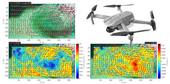
The aerial video data were taken by a DJI Mavic quadcopter with a self-stabilized gimbaled 1/2.3″ CMOS-sensor providing 4K video recording (4096-by-2160 pixel frame, 24 frames per second). The vertical and horizontal field-of-view angles, estimated from analysis of a calibration scene, are 42${}^{\circ }$ and 72${}^{\circ }$, respectively.

The measurements were made at the western coast of the Crimean Peninsula (Sevastopol), mostly in upwelling-favorable wind conditions over a bay outlet having two entrance piers. The coastline to the north of the bay has a predominantly meridian orientation. Hence, the northerly winds frequently induce upwelling events due to a water flow directed offshore (to the west). The accompanying storm waves cause clay cliff abrasion resulting in a dramatic increasing of coastal water turbidity. These waters are entrained into a strong frontal current formed on the periphery of the upwelling and directed to the south [32].

For the present study, we have selected four flights during three different days in 2020–2021 (

Table 1. Flight timetable, look geometry, and wind conditions reported by a local weather station.

Scene	Local Time	Duration ${}^1$	Height	Incidence	Wind Speed	Wind Gusts	Wind Direction
#	[UTC+3]	[s]	[m]	Angle ${}^2$ [${}^{\circ }$]	[m s${}^{-1}$]	[m s${}^{-1}$]	[rhumb]
1	16 February 2021 12:44	245	500	22.9	8	12	NE
2	9 July 2020 12:13	110	436	29.9	7	10	NNW
3	23 July 2021 13:11	120	500	31.5	8	10	N
4	23 July 2021 15:31	140	226	0.5	8	10	N

¹ the duration of the processed video fragment, ² the angle between camera line-of-sight and a vertical line.

). The above-mentioned upwelling signatures are clearly recognized in the corresponding Aqua/MODIS sea surface temperature shown in Figure 1a–c with a maximum possible one-day lag for a better cloud mask. The upwelling waters are clearly seen in the satellite data as a cold nearshore band around the southwestern coast of the Crimean Peninsula (Figure 1a,b) with an exception for the winter season (Figure 1c) showing a less prominent near-shore feature.

The experiment site and analyzed scenes are shown in Figure 1d,g,j,m based on the UAV images. All four scenes exhibit a turbid band feature extended from north to south along the coast, resembling the satellite data but at much higher resolution. The high-resolution UAV image revealed eddies to the west of the bay in Scenes #2,3,4 suggesting a current directed out of the bay. The coastal dynamics in these UAV images is clearly visualized thanks to the mixing of the clear bay waters and highly turbid upwelling waters. All measurements were made in similar wind conditions, roughly at the same area with depths of about 15–17 m (indicated by red boxes in Figure 1).

The video records were cropped to the time intervals when the UAV was self-stabilized, i.e., when no commands from the pilot were issued. In this mode, the camera pitch/roll/yaw angles, provided by the UAV inertial motion unit (IMU), were found constant within its $0.1^{\circ }$ measurement accuracy with zero roll angle. Thus, the projection transform applied to the whole fragment is constant and is only determined by the incidence (pitch-90${}^{\circ }$) angle, $\theta$, and UAV height.

The 10-min mean wind speed measured at 10-m height was reported by the nearest weather station, WMO33994 Cape Chersonese, 10 km west of the experiment site.

2.2. Wave Dispersion Analysis (WDA)

The current estimation is based on the surface wave dispersion analysis (WDA). Different variations of this approach are widely used for surface current and bathymetry retrievals [25,26,27]. In brief, the approach is based on the surface wave phase velocity dependence on both water depth and surface current velocity, the well-known linear wave dispersion relation,

$$\omega =\sqrt{gktanh\left(kD\right)}+\mathbf{k}·\mathbf{U},$$

(1)

where g is the gravity acceleration, $\omega$ is the angular wave frequency, $\mathbf{k}$ is the wave vector, D is the water depth, and $\mathbf{U}={\int }_{-\infty }^0\mathbf{u}\left(z\right)exp\left(2kz\right)dz$ is the integrated sea surface current (SSC) weighted with the exponential function over the current profile, $\mathbf{u}\left(z\right)$. For the currents monotonically decaying with depth, $\mathbf{U}$ can be approximated by the effective current in the upper 1/2k-thick layer [33]. Where deep water approximation is applicable and vertical current shear is ignored, the inversion of Equation (1) can be reduced to solving the linear equation system,

$${\omega }_i=\sqrt{g{k}_i}+{\mathbf{k}}_i·\mathbf{U},$$

(2)

where ${\omega }_i$ and ${\mathbf{k}}_i$ are the set of observed wave frequencies and wave vectors, respectively. At least two non-collinear wave components are necessary to determine the SSC vector, $\mathbf{U}$. At best, a fully isotropic wave field would provide the minimal SSC ambiguity. Thus, the more isotropic short wind waves are preferable for better SSC estimates. At the same time, analyzing shorter waves can provide a better spatial resolution of the estimated SSC maps.

The estimation of ${\omega }_i$ and ${\mathbf{k}}_i$ is performed in the Fourier wavenumber-frequency domain. The critical issue of the WDA applied to optical images is rejecting spurious spectral peaks generally related to the non-linearity of the “sea surface-to-image” transfer function. The main source of non-linearity in optical data is the sun glints. At first glance, the glints may be avoided with a proper look geometry. However, this would also significantly reduce the optical wave contrast and signal-to-noise ratio because the direct sun reflection is the main wave imaging mechanism for near-nadir look geometry, when reflected skylight is weak. From our experience, the best results for WDA are achieved when sun glints are present in the scene.

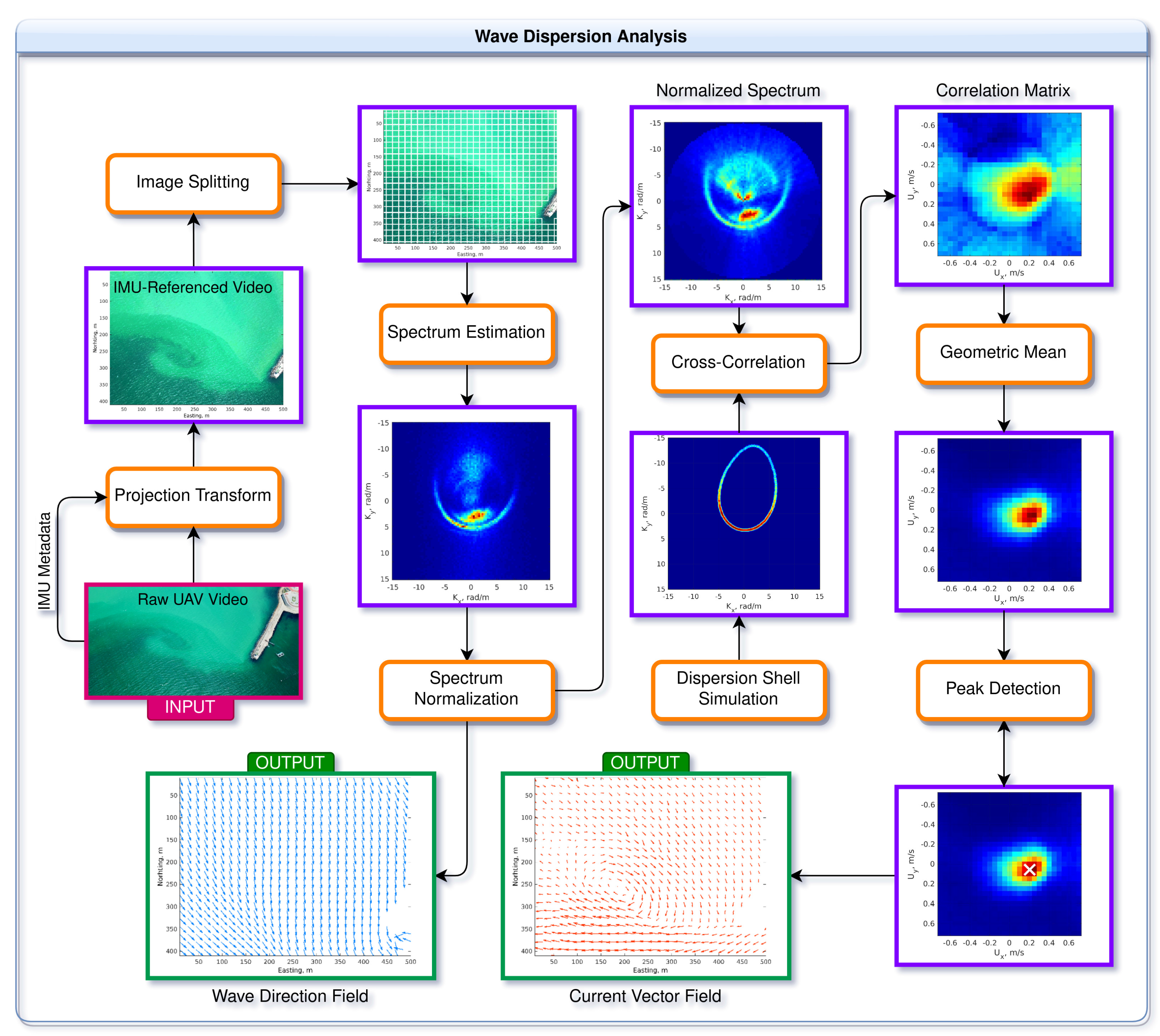
To analyze such images, and which spectra have strong spurious harmonics, we use the WDA version developed for the optical images taken from a research tower [29]. The method is based on the analysis of 3D-Fourier spectrum frequency slices, or wavenumber spectra at a given frequency (Figure 2). These slices have dispersion shell signatures in $(k_x,k_y)$-space: a circle for $U=0$, or an ellipse-like curve otherwise. The non-linear harmonics, along with fundamental mode, also respond to the current but at different wavenumbers. The present WDA approach is optimized for recognizing the fundamental mode in the spectrum frequency slices. The method involves the following steps:

1.

Georeferencing the image sequences. Video frames are projected on the horizontal plane using intrinsic camera parameters and IMU flight metadata, incidence angle, $\theta$, and UAV height, H. For slant look geometry, the resulting resolution varies within the frame area, fine/coarse at near/far zone. Thus, the image is interpolated to the constant 20-cm spatial resolution corresponding to the near-zone maximal resolution at $H=500$ m, $\theta ={20}^{\circ }$. Following [34], the red channel data is analyzed to minimize the scattered light contamination (mostly blue or green), and thus increase wave imaging contrast.

2.

Splitting the georeferenced video into n-by-n-by-m data blocks, where n is the number of pixels and m is the number of frames in the video. The data block size, n, was set to 100 pixels corresponding to a 20-m resolution of the resulting current map. The total number of frames, m, determined by the record duration and framerate (24 Hz), was varying from 2640 to 5880 for different scenes (see Table 1).

3.

Computing the spatio-temporal power spectrum of the data blocks. The squared magnitude of the 3D Fast Fourier Transform is used for the spectrum estimation.

4.

Spectrum normalization. The most energetic waves travel in the wind direction. Yet, some portion propagating off the wind is important for accurate current vector estimation. To equalize this azimuth contrast, and thus improve the dispersion shell recognition, the spectrum is normalized by its mean value in each azimuth direction, $\tilde{S}(\omega ,k,\theta )=S(\omega ,k,\theta )/\int S(\omega ,k,\theta )dk$. The “by-product” of this procedure is the wave direction at a given frequency, $\overline{\theta }\left(\omega \right)=\int \theta S(\omega ,k,\theta )dkd\theta /\int S(\omega ,k,\theta )dkd\theta$.

5.

Simulating the Doppler-shifted power spectra in the expected SSC limits. Spectrum frequency slices are simulated for the expected SSC vectors. For our Black Sea coastal measurements, the SSC is varied within $U<1$ m s${}^{-1}$ with a 0.05 m s${}^{-1}$ step. The simulation is performed by adding a unit to the initially zeroed spectrum slice cells corresponding to wave components spanning all possible (0–360${}^{\circ }$) azimuths with a 0.1${}^{\circ }$-step and satisfying Equation (2). The angular energy spreading is ignored for this simulation. Yet, for strong SSC magnitudes, the simulated dispersion curve is dense/sparse for the wave directions opposite/co-aligned to the SSC vector due to the finite 0.1${}^{\circ }$-step between simulated components.

6.

Computing the cross-correlation between measured and simulated spectrum frequency slices for all possible $\mathbf{U}$ values for each data block. The resulting correlation matrix, $C(\omega ,\mathbf{U})$, provides a measure of similarity between measured and theoretical dispersion shell slices. At a given frequency, $\omega ={\omega }^{\prime }$, the correlation matrix, $C({\omega }^{\prime },\mathbf{U})$, reflects the current averaged over the 1/2k-thick upper layer ($k={\omega }^{\prime }{}^2/g$). For our high-resolution 20-m data, the low-frequency cut-off, corresponding to half the block size, $\lambda =10$ m, equals ∼0.4 Hz. The high-frequency cut-off, determined by the spatial sampling scale, 20 cm, equals ∼2 Hz. However, from our previous experience [29], the practical cut-off is about 1 Hz, first, due to the short-wave Doppler smearing by orbital motions of longer waves, second, because the reprojected image resolution in the far zone is artificially interpolated to 20 cm. Thus, to save computation time, the cross-correlation matrices, as well as simulations on the previous step, are performed only for the frequencies within the 0.5–0.9 Hz interval, corresponding to effective SSC in the 0.5–0.12-m-thick upper layer.

7.

Spectral averaging of cross-correlation matrices. Ignoring the possible vertical current profile for the analyzed frequencies (<$0.5$ m in terms of effective depth), the cross-correlation matrices are averaged over $\omega$. The better results are achieved for geometric mean estimates, $\overline{C}\left(\mathbf{U}\right)={\left[{\prod }_{i=1}^{N}C({\omega }_i,\mathbf{U})\right]}^{1/N}$. This is explained by the fact that spurious peaks in $C(\omega ,\mathbf{U})$ matrices are mismatched and cancel out when the matrices are multiplied. The true current peak is always in the same place, within the ignored vertical current variability error. Thus, the geometric mean procedure “focuses” the true peak of the cross-correlation matrices (see Figure 3 in [29]), corresponding to the depth-mean current (∼0.5 m in our case).

8.

Cross-correlation peak detection. The sea surface current (SSC) vector is estimated from the first moment of mean correlation matrix, $\overline{C}\left(\mathbf{U}\right)$, which is first zeroed below the level corresponding to some portion, $\epsilon$, of the matrix maximum. This helps to better estimate the peak position but introduces the only tuning parameter of the method the level of which is set heuristically to $\epsilon =0.85$. The SSC root-mean-square error (RMSE) is estimated from the second moment of $\overline{C}\left(\mathbf{U}\right)$.

3. Results

Applying the WDA to the quasi-stationary flight video records yields SSC vector fields and its RMSE. For better visualization, we also display the SSC magnitude and vorticity contour plots. The “bonus” wave directions, averaged over the same frequency interval as SSC, 0.5–0.9 Hz (wavelengths 2–6 m), are shown by unit vector quiver maps. The results are presented in ascending order of complexity, not chronologically.

3.1. Scene #1

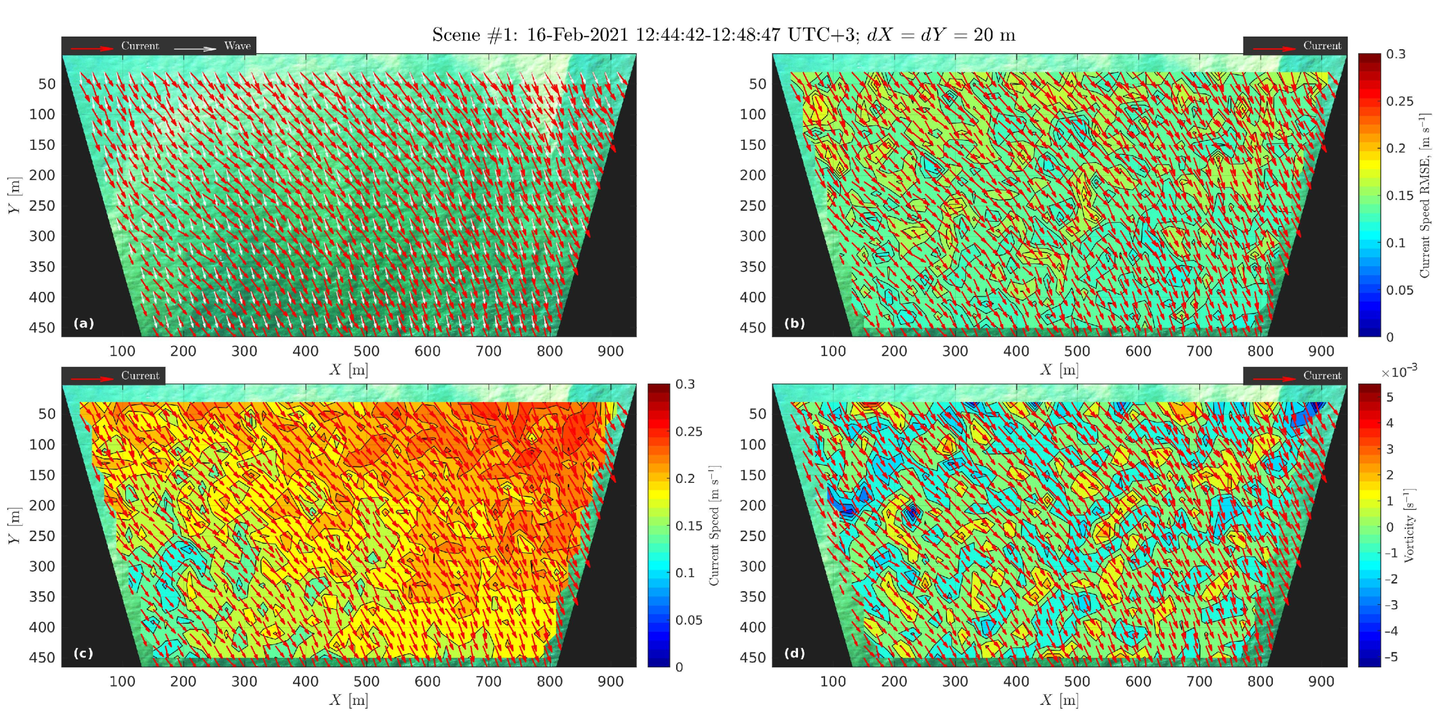
We begin with the relatively “plain” situation captured in winter season on 16 February 2021, Scene #1 (Figure 1d–f). The measurements were taken after a northwesterly storm observed on 13 February 2021. During the flight, the wind speed was ∼8 m s${}^{-1}$ with gusts up to 12 m s${}^{-1}$ (see Table 1). The turbid alongshore band pattern, striped and generally nonuniform, was well-seen in the UAV data including the analyzed area.

The estimated SSC direction (Figure 3a) was rather uniform within the image and generally was directed to the south-southeast. The SSC magnitude (Figure 3c) increased towards the upper-right image corner. This somehow corresponded to the visually observed features in Figure 3a: the turbidity contrast was stronger on the onshore side of the turbid band presumably associated with along-shore current. The SSC vorticity was noisy and did not exhibit any specific eddy-like features (Figure 3d) in agreement with visual inspection of the optical images.

The SSC RMSE, about $0.15$ m s${}^{-1}$, was also rather uniform over the image (Figure 3b) and reached ∼50% of the total SSC magnitude. Wave directions were generally co-aligned with the SSC and were also quite uniform.

3.2. Scene #2

Scene #2, acquired in the 2021 summer season, on 9 July 2021, followed a strong northwesterly wind event blowing one day before. This time the high-resolution UAV data (Figure 1g–i) revealed a vortex street located on the northern side of the bay entrance consisted of three submesoscale anticyclonic eddies. The diameters of the eddies increased with the distance from the pier and were about 100 m, 200 m, and 400 m, respectively. Consecutive flights made between 12:00 and 14:00 UTC+3 showed that the eddies traveled to the west with a translational speed of about 0.10 m s${}^{-1}$. Scene #2 captured one of these eddies.

Applying the WDA to this scene revealed an anticyclonic eddy in the SSC map well matched with the optical image (compare Figure 1i and Figure 4a). Apparently, this eddy was generated by a jet-like current ∼0.15–0.20 m s${}^{-1}$ directed to the west (out of the bay, Figure 4c). Relatively clean bay water mixed with turbid coastal water causing strong turbidity gradients in this scene (Figure 1g–i). Encountering a topographic obstacle (pier), this jet generated an anticyclonic eddy entraining surrounding turbid waters that made the eddy visible in the image color/brightness. This is confirmed by the vorticity field exhibiting a prominent positive feature at the right boundary of the jet (Figure 4d).

A probable reason for this outflowing current is the upwelling motion causing a sea level difference between the open sea and the bay. In the northern part of the scene, shadowed by the pier, the currents are near zero. The strong shear between the outflowing current and still waters behind the pier forms an extended band of enhanced positive vorticity exceeding 0.003 s${}^{-1}$. In this area, an anticyclonic eddy is formed with a maximum value of vorticity in its core reaching 0.005 s${}^{-1}$, or ∼50f, where f is the Coriolis frequency. The center of the eddy corresponds well with the anticyclonic turbidity pattern seen in the optical image.

The SSC RMSE for this scene (Figure 4b) is significantly lower than for the previous one, probably due to the lower ∼500-m wind speed which is expectedly correlated with the 10-m wind speed reported by the local weather station (Table 1). The RMSE field is again negatively correlated with the SSC magnitude (compare Figure 4b,c). Particularly, the increased vorticity area is slightly replicated in the RMSE field (compare Figure 4b,d). This is explained by the strong directional variability of the SSC vectors spanned by the same data block at the jet boundary.

In contrast to Scene #1, the waves demonstrate a more complex directional behavior. Being generally directed to the south-east, they turn somewhat counterclockwise in the left bottom corner of the image and “swirl” around the pier.

3.3. Scene #3

This scene was observed almost in the same conditions as Scene #2, but about a year later, on 23 July 2021. The similar vortex street was observed behind the northern side of the bay outlet (Figure 1j–l). The vortex street in this scene consisted of four visible anticyclonic eddies, while up to six eddies at once were observed simultaneously during the measurements on that day. From our experience, the eddies traveled along the turbid front to the west (similarly to Scene #2, downstream the current outflowing the bay) with a translational speed ∼0.1 m s${}^{-1}$. Sometimes we visually observed a strong intermittency of the vortex street indicating pulsating nature of the outflowing current responsible for the eddy formation (notice a gap in the vortex street in Figure 1k). Scene #3 spans the time interval when the current was at the strong pulsation phase as can be anticipated from the oblate shape of the eddies.

The outflowing current is clearly seen in the resulting SSC map (Figure 5c) as a jet confided between the piers. The current speed, ∼0.2 m s${}^{-1}$, was maximal in the narrowest place of the bay outlet and vanished behind the piers. Again, such strong horizontal current shear was the most plausible reason for the generation of the observed eddies. The right boundary of the current was somewhat meandering but the eddies were not well resolved in the SSC map. This is explained by the finite, ∼2 min, time averaging interval which smooths the non-stationary eddies traveling down the vortex street. For example, during this period, a ∼30 m-eddy having ∼0.1 m s${}^{-1}$ translational speed (the smallest in the observed street), shifts by almost half-size, and thus is smoothed in the resulting SSC map.

The vorticity map is very similar to that of Scene #2, exhibiting a positive area at the right jet boundary. Note that though the left jet boundary is not traced by turbid waters, a negative vorticity area is nonetheless seen in the vorticity map. This probably suggests a symmetric generation of cyclonic eddies on the left side of the outflowing current which are not seen due to the absence of optical gradients.

The SSC RMSE (Figure 5d) was again higher at the weak current area than within the jet.

3.4. Scene #4

The next Scene #4 (Figure 1m–o) was captured two hours after Scene #3 over one of the vortex street eddies at near-nadir look geometry and a twice less height for a better spatial resolution (Table 1). During this flight, the outflowing current was weaker than during Scene #3, as hinted by a more symmetrical shape of the eddy. The structure of this ∼300 m eddy is perfectly seen in the field of suspended matter. The eddy entrained turbid waters in its northern part (bottom of the image) and clean waters in its southern part (top of the image). Clean and turbid waters moved in a spiral pattern and mixed near the eddy core where the optical gradient decreased.

The SSC reconstruction using WDA successfully reproduced the anticyclonic circulation within the scene (Figure 6). The eddy had a 50-m diameter near-zero SSC “eye” which corresponds to the visual position of the eddy center. The maximum orbital velocity on the eddy periphery, ∼100 m away from the eddy core, was about 0.12–0.14 m s${}^{-1}$. Strong velocity gradients on such small spatial scales caused a peak in the vorticity field (Figure 6d) in the eddy center reaching 0.01 s${}^{-1}$, or about 100f, indicating highly nonlinear dynamics of the eddy.

The wave direction field was again distorted, and this distortion is clearly correlated with the SSC maps (Figure 6a,b). The SSC RMSE was somewhat higher for the low current magnitude areas, e.g., in the eddy eye, and it was also controlled by the wave-to-current direction, as it can be deduced from the crest-like feature co-aligned with the eddy (Figure 6b).

3.5. Root-Mean-Square Error

The error of the WDA method, the RMSE shown in panel (b) of Figure 3, Figure 4, Figure 5 and Figure 6, is estimated as a peak width of a correlation matrix. This error estimate is determined up to a scale factor because of zeroing the correlation matrices below the empiric threshold, $\epsilon$, that helps to distinguish between the true SSC peak and noise. Thus, with the RMSE defined in this way, the absolute error is undetermined, but we can assess the error distribution over SSC maps. Generally, the estimated SSC RMSE is higher/lower in weak/strong current areas. This can be explained by the following speculations.

The present WDA method relies on the recognition of dispersion curve signatures in 3D-spectrum frequency slices. In other words, on the recognition of a specific curve in the $(k_x,k_y)$-space. Thus, the error of the method is determined, first, by the wavenumber resolution $\delta k=2\pi /dX$, where $dX$ is the SSC map resolution, and, second, by the sensitivity of the dispersion curve to SSC, $|\partial U/\partial k|\delta k$. An illustration is given in Figure 7 showing dispersion curves at $f=0.7$ Hz for different SSC magnitudes, $0,0.20,0.40$ m s${}^{-1}$, perturbed within $\pm 0.05$ m s${}^{-1}$ limits.

As understood from Equation (1), the waves coming obliquely to SSC ($k_x=0$ in Figure 7) are not Doppler-shifted, and thus are useless for SSC retrieval. The waves co-aligned with SSC ($k_x>0,k_y=0$ in Figure 7) are responsive to the latter, but the best sensitivity appears for the waves opposite SSC ($k_x<0,k_y=0$ in Figure 7). For these two cases, the error can be explicitly derived from Equation (1),

$$\frac{\partial U}{\partial k}=\pm \sqrt{\frac{g}{4k^3}}\mp \frac{\omega }{k^2}.$$

(3)

For a quite strong SSC magnitude, $U=0.5$ m s${}^{-1}$, the typical SSC map 20 m resolution, $\delta k=0.3$ rad m${}^{-1}$, and the middle frequency used in our WDA algorithm, $f=0.7$ Hz, the error estimate based on Equation (3) is ∼0.4 m s${}^{-1}$ and <0.01 m s${}^{-1}$ for co-aligned and opposite waves, respectively.

The real error is indeed much more complex because the recognition algorithm relies on a variety of wave-to-current directions, which, in turn, is determined by the wave spectrum directional spreading and the “slope-to-brightness” transfer function. However, the present first-guess error analysis is able to qualitatively explain the inverse relation between the SSC RMSE and the SSC magnitude. The increased RMSE for Scene #4 (Figure 6c) is also explained by the finer SSC map resolution, $dX=10$ m, and hence coarser wavenumber resolution, $\delta k\sim 0.6$ rad m${}^{-1}$, and thus worse RMSE.

Notice, the rather inconvenient non-linear error, Equation (3), can be avoided if the dispersion curve recognition is performed in $(\omega ,\varphi )$-space. Indeed, for a fixed wavenumber, $k=\mathrm{const}$, the dispersion shell cross-section is a cosine-like curve, $\omega \left(\varphi \right)=\sqrt{gk}+kUcos\varphi$, and the error is inversely proportional to wavenumber, $|\partial U/\partial \omega |\delta \omega \sim 1/k$. The SSC estimate would be even further improved, if the recognition is performed in the 3D $(k,\omega ,\varphi )$-space. This, however, would require additional computational efforts and for the present demonstration study we use the simplest approach and analyze only the spectrum frequency slices.

3.6. UAV Drift

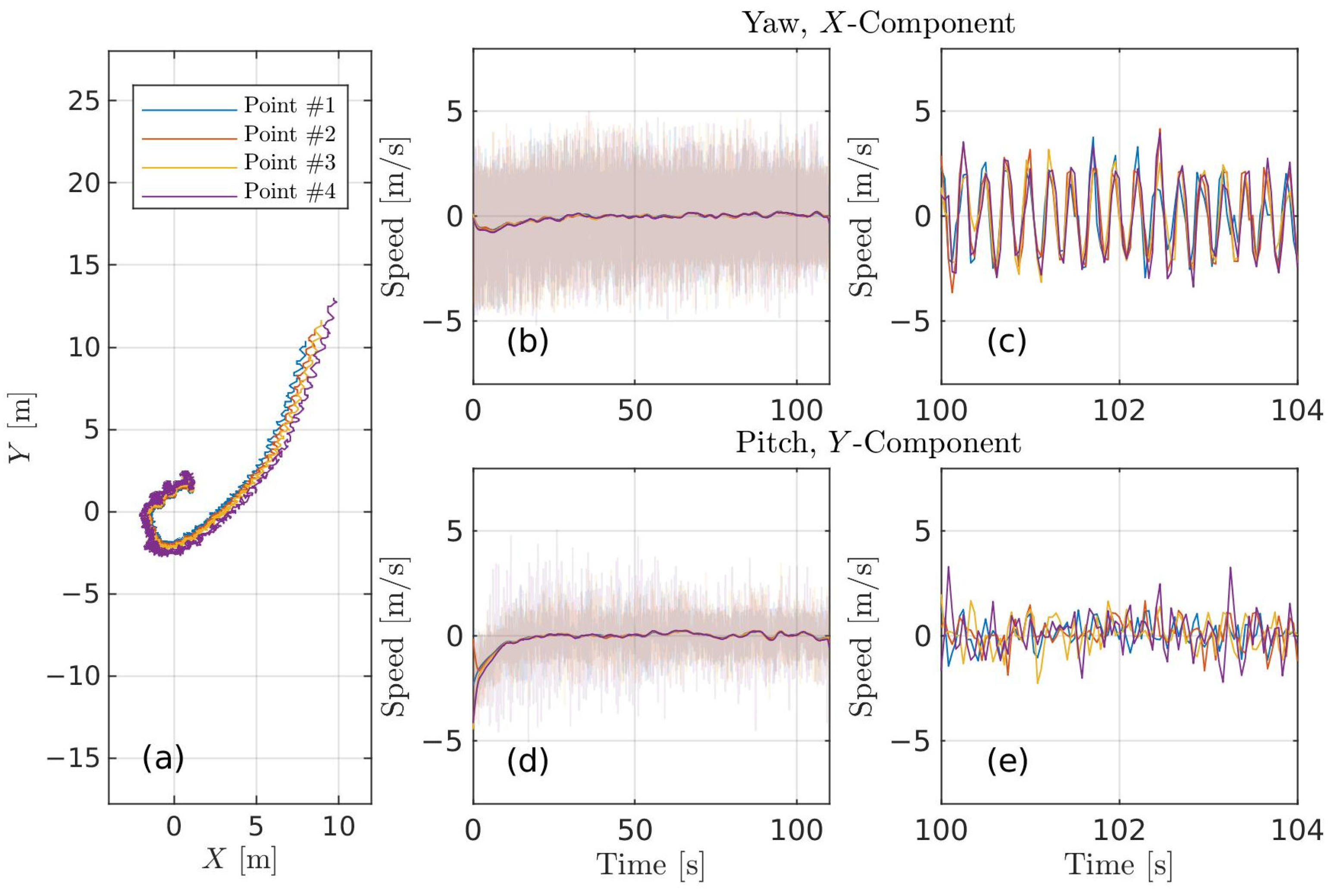
The accuracy of UAV self-stabilization is crucial for current retrieval. Both uncontrolled drift and rotations distort the true current for the observer in the UAV reference frame. To check the UAV self-stabilization quality we used land objects best captured in Scene #2. Four control points at the pier were traced using image cross-correlation analysis (Figure 8).

We found that, after a ∼10-s relaxation period, the control point velocity stabilized with a ∼2 m s${}^{-1}$ standard deviation and a well-pronounced ∼4-Hz oscillation in yaw direction. This noise, quite strong relative to a typical current magnitude, smeared the dispersion curve spectrum signature, similarly to long-wave orbital motions, and thus increased the RMSE of the SSC estimate, but it is averaged out from a time-average estimate. The really important mean control point velocity was <0.1 m s${}^{-1}$ for the whole fragment, and would be <0.05 m s${}^{-1}$, if the relaxation period was excluded. We also processed the video records matched to the control points using a non-reflective similarity transform and found no significant changes in the final SSC maps.

This test of the IMU-referencing quality shows that for wind speed 7–10 m s${}^{-1}$, our particular UAV model can be used for SSC retrieval with 0.05–0.1 m s${}^{-1}$ accuracy. Further investigation of UAV self-stabilization capabilities at different wind speeds, altitudes, UAV models, not planned for this study, is desirable to understand in detail the wind limitations for the SSC retrieval using UAVs.

3.7. Intercalibration with 4D-Variational Assimilation Method

In absence of ground truth data for the present data set, we use the alternative well-established 4D-variational assimilation (4DVAR) method for a possible intercalibration with the WDA method. The 4DVAR, based on the analysis of the optical tracer field evolution, allows current reconstruction from two or more consecutive images. We applied the 4DVAR implementation presented in [30] for satellite images to Scene #2 containing both eddy-like and jet-like structures. Briefly, this method includes the following steps:

1.

Image pair selection. The 4DVAR is performed for seven pairs of UAV images spaced by 12.5 s. The images within the pairs are spaced by 25 s, i.e., the pairs are half-overlapping in time. In contrast to WDA, the green channel is analyzed because of a higher clean/turbid water contrast.

2.

Percentile filtering. Removing brightness modulations from surface waves with a 45 × 45 pixel sliding filter that passes a 30-percentile of the signal.

3.

Histogram matching. Performing image-to-image contrast adjustment that matches empirical brightness cumulative distributions of both images [30].

4.

4D-variational assimilation. The image pairs are fed to the 4DVAR procedure [31] involving inversion of the optical flow equation,

$$\frac{\partial I}{\partial t}+u\frac{\partial I}{\partial x}+v\frac{\partial I}{\partial y}=0,$$

(4)

that iteratively minimizes the cost function,

$$J=\frac{1}{2}\sum _{k=1}^N{\int }_{\Omega }{(I\left(t_k\right)-I^{\prime }\left(t_k\right))}^{2}ds+\frac{\alpha }{2}{\int }_{\Omega }{\left|\mathrm{grad}\mathbf{U}\right|}^{2}ds+\frac{\beta }{2}{\int }_{\Omega }{\left(\mathrm{div}\mathbf{U}\right)}^{2}ds,$$

(5)

where I is the observed image brightness, $I^{\prime }$ is the simulated image brightness, $\mathbf{U}=(u,v)$ is the velocity field assumed to be stationary, $\Omega$ is the observed area, N is the number of observations, $\alpha$ and $\beta$ are the empirical constants, and $t_k$ is the observation time. The first term in Equation (5) compares observations and simulations, the second and the third terms provide regularization to avoid aperture effects (more details can be found in [31]).

The 4DVAR applied to the Scene #2 images (Figure 9) yields the SSC map qualitatively similar to the WDA method: in both cases an anticyclonic eddy behind the pier and the outflowing jet current signature are clearly resolved. Yet, there are some distinct differences. The 4DVAR-derived current in the turbid water area (top of the image) is not so strong as on the WDA-derived SSC map. A somewhat different SSC magnitude distribution over the jet area (bottom of the image) also results in a less pronounced vorticity peak corresponding to the eddy center. The distinctions can be explained by the different input information used by the methods. The 4DVAR is based on the tracer evolution analysis while the WDA relies on surface waves. Therefore, the 4DVAR output lacks details in the very clear or very turbid water areas with low optical gradients. Apparently, 4DVAR can complement WDA in calm wind conditions (no visible waves) with only the requirement for passive optical gradients tracing the currents.

4. Discussion

Despite possible errors, the relevance of the SSC estimates is implicitly supported by a good agreement with visually observed tracer fields. With our approach, the coastal submesoscale currents can thus be reconstructed and analyzed at a fairly fine resolution, O(10–20 m). Using the present training data set, resolving such small scale coastal dynamics, some interesting oceanographic aspects can be noticed.

4.1. Eddy Dynamics

In the experiment, we detected a current flowing out of the bay in line with the surrounding upwelling event. The two piers sheltering the bay possibly amplify this jet-like current reaching 0.20–0.25 m s${}^{-1}$ magnitude in the narrowest place. A strong horizontal shear behind the piers led to the generation of a structure similar to the von Karman’s [23] vortex street which was opportunely traced by turbid waters at the right boundary of the jet. The observed vortex street consisted of 3–6 eddies traveling downstream at a ∼10 cm/s translational speed. The individual eddies in the street had an anticyclonic direction, a diameter of ∼200–400 m, and an orbital velocity about 0.15–0.30 m s${}^{-1}$, corresponding to a Rossby number, $\mathrm{Ro}=w/f\sim 15$, where w is the vorticity and f is the Coriolis frequency. Surprisingly, this is much higher than the critical Rossby numbers observed in laboratory, e.g., $\mathrm{Ro}=4.5$ for cyclones and $\mathrm{Ro}=0.65$ for anticyclones [35], or in numerical experiments, e.g., $\mathrm{Ro}=1.65$ for cyclones and $\mathrm{Ro}=0.57$ for anticyclones [36].

Kloosterziel and van Heijst [35] suggest that the Rossby number for anticyclones, in contrast to cyclones, cannot reach high values due to the cyclostrophic instability destroying the anticyclones. Our results suggest that the intense anticyclones, $\mathrm{Ro}\sim 15$, indeed may exist in a complex coastal environment for up to one hour (from visual observations).

This is speculatively explained by the outflowing current feeding the eddies and the presence of confining boundaries (the coast and the upwelling front, see Figure 1g,j,m) preventing the anticyclonic widening due to centrifugal forces.

The strong vorticity in such stabilized eddies may induce strong downwelling with corresponding impacts on coastal vertical circulation and exchange processes. Hence, our observations demonstrate the highly nonlinear character of coastal eddies and the important role of centrifugal forces on their dynamics.

4.2. Wave-Current Interaction

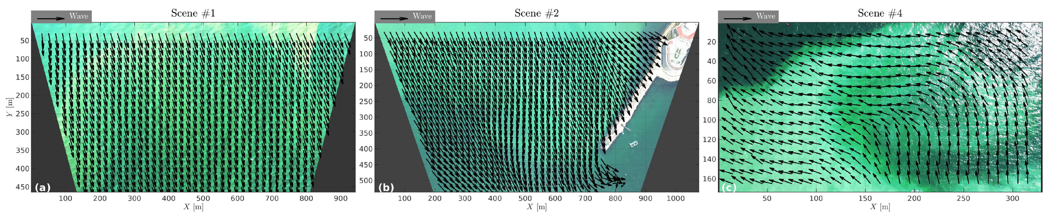
The proposed WDA method is beneficial in its capability to estimate both currents and waves simultaneously, if the latter are present on the sea surface. Noticeably, small-scale currents have larger effects on waves [37] while small-scale waves are more sensitive to currents [38]. Thus, the high-resolution UAV-derived SSC and wave maps, similar to those presented in this study, can provide new knowledge aiding in wave-current interaction studies. To demonstrate this, we show the effects of wave refraction for Scene #1 without current gradients and Scenes #2,4 with strong current gradients.

In contrast to an almost uniform wave direction field observed for uniform SSC (Figure 10a), wave direction varies noticeably in the presence of eddies (Figure 10b,c). Some portion of this variability can be speculatively attributed to the coastal wind distortions and bottom effects (Figure 10b, the area around the pier). For instance, the minimal wave frequency, $f=0.5$ Hz, involved in the present WDA realization corresponds to wavenumber, $k\sim 1$ rad m${}^{-1}$, and the $tanh\left(kD\right)$-factor in Equation (1), responsible for bottom effects, is $tanh\left(kD\right)<0.9$ for $D<1.5$ m.

This latter estimate also suggests that the bottom effects cannot explain the wave direction field deformation observed over the Scene #2,4 eddies (Figure 10b,c) where the bottom depth is about $D\sim 15$ m, i.e., $(1-tanh\left(kD\right))<{10}^{-12}$. In these cases, the waves are first refract to the right of the eddy center and then to the left. This vaguely resembles numerical wave ray simulations reported by Kudryavtsev et al. [39] (see their Figures 14 and 15 showing swell trapping in a meander of the Agulhas Current) and by Rapizo et al. [40] (see their Figure 11 showing waves refracting on a mesoscale eddy).

In the case of Scene#2 (Figure 10b), the waves do not exhibit a visible refraction on the outflowing current. In contrast to the ocean swell simulations in the Southern Ocean [39,40], the waves analyzed here are much shorter, $\lambda \sim 6$ m, and hence are much more responsive to the wind field inhomogeneities which may play a role in the wave direction distribution.

Finally, the short-wave energy modulation by current gradients, estimated from image brightness modulation, can also be potentially accessed with the proposed UAV imagery processing framework. We leave this discussion open for further research.

5. Conclusions

A commercial unmanned aerial vehicle (UAV) quadcopter is used for estimating sea surface current (SSC) over the coastal area of the Crimean peninsula. The measurements were conducted during upwelling events with increased water turbidity due to abrasion of a nearby clay cliff. The turbid water, when mixing with clear water, acts as a tracer and makes the coastal dynamics visible. Guided by the appearance of such turbid structures, several UAV flights were performed over a bay outlet where eddy-like structures were occasionally observed.

The video records were processed using wave dispersion analysis (WDA) widely applied for SCC and bathymetry estimation from ocean surface wave images [25,27,41]. The feature of the present WDA implementation is the optimized dispersion shell recognition aimed at discarding false spectral peaks caused primarily by the non-linearity of the wave imaging mechanism [29].

In the presence of turbid “look-alike” frontal features, the WDA-derived SSC maps reveal both homogeneous and vortex structures disclosing the dynamics hidden to the naked eye. The alternative 4D-variational assimilation (4DVAR) method of current estimation [30,31] was also tested and showed very similar results with somewhat less details in the areas with weak optical contrast (very clear or very turbid water). This suggests that 4DVAR can complement WDA in calm wind conditions when waves are too short to be resolved by the UAV camera.

From our experience, the UAV self-stabilization capability is the most challenging issue in the SSC reconstruction. One of the scenes with static land control points, performed at 500-m height under 7–10 m s${}^{-1}$ wind speed measured at 10-m height, was used to estimate the possible errors related to the uncontrolled platform motions. We found that, for our present UAV model, the standard deviation of the reprojected ground velocity is ∼1 m s${}^{-1}$ in pitch direction and ∼2 m s${}^{-1}$ in yaw direction. These motions, dominated by the variations of the camera look direction, are of the same order of magnitude as orbital motions of typical ocean long waves. Comparing the SSC maps retrieved from the image sequences with and without land referencing, we found no significant difference between them. The mean drift velocity is ∼0.1 m s${}^{-1}$, but can be reduced to ∼0.05 m s${}^{-1}$, if the $\sim 10$-s relaxation period is excluded from the processing.

Based on the present data set, we demonstrate the potential of a commercial UAV in submesoscale and even smaller scale oceanographic investigations. The dynamics of the coastal eddies observed in quite a complex coastal environment is reconstructed and discussed. With a diameter of ∼200–400 m and ∼0.15–0.30 m s${}^{-1}$ orbital velocity, such eddies have surprisingly high vorticity (the Rossby number $\mathrm{Ro}\sim 15$), and thus may have significant impacts on vertical circulation, energy transfer between large-scale motions and small-scale turbulence, and suspended matter transport. Furthermore, the presented SSC estimation approach can be combined with wave measurements to study the wave–current interaction processes, as revealed from our observations of short-wave refraction on the current gradients in the detected eddies.

With further progress in UAV technologies, their extensive involvement in coastal oceanography practice is expected both for academic needs and emergency operations (oil spills, surges and floods, beach morphology monitoring). Our findings suggest that, already today, the self-stabilization capabilities of modern multi-rotor copters allow the sea surface current retrieval in, at least, moderate wind conditions without land referencing. Thus, the measurements made by a commercial multi-copter UAV on a research cruise can possibly shed some light on the still unresolved submesoscale open ocean dynamics.