Article

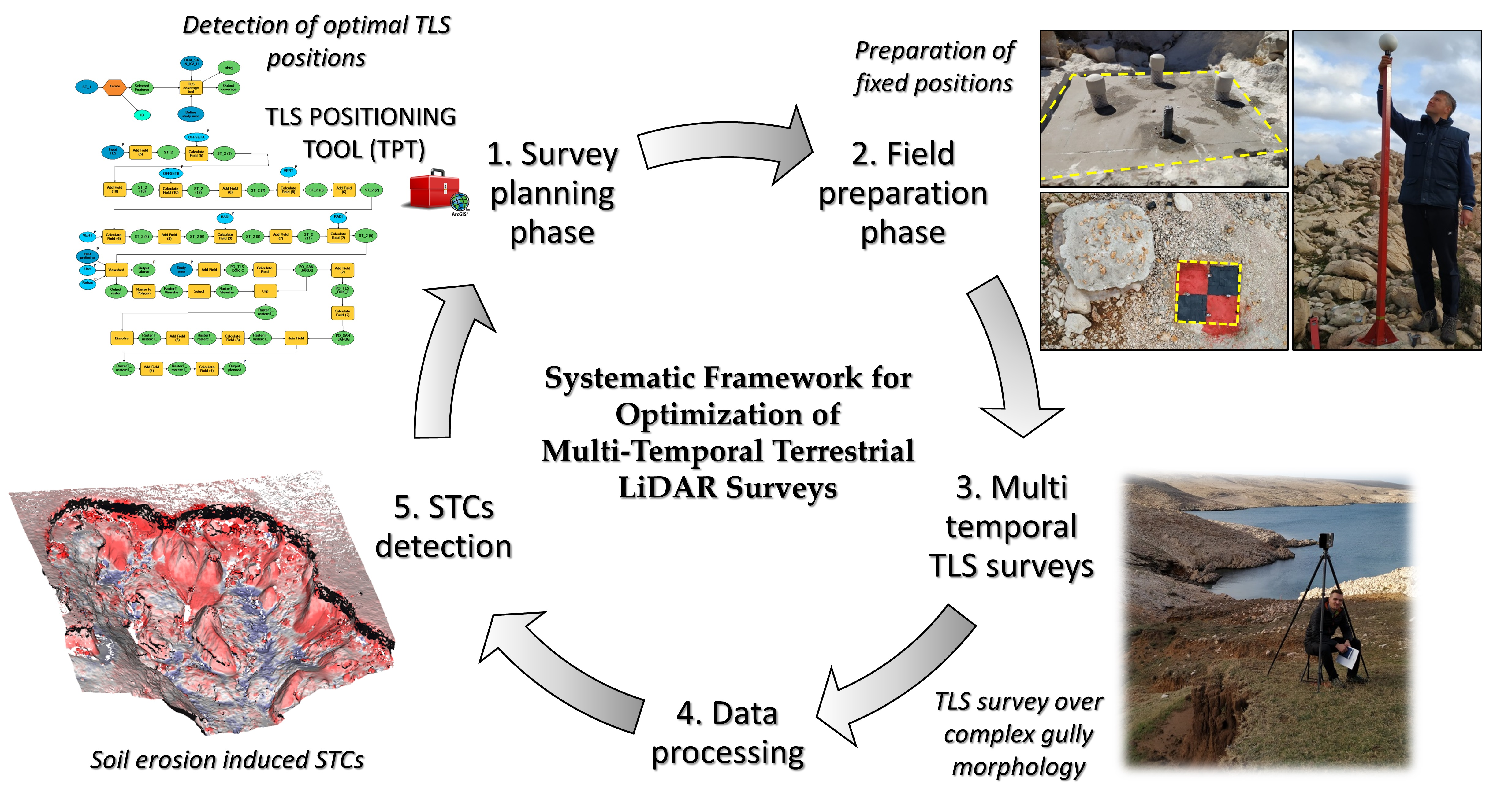
A New Systematic Framework for Optimization of Multi-Temporal Terrestrial LiDAR Surveys over Complex Gully Morphology

Department of Geography, University of Zadar, 23000 Zadar, Croatia
*
Author to whom correspondence should be addressed.
Remote Sens. 2022, 14(14), 3366; https://0-doi-org.brum.beds.ac.uk/10.3390/rs14143366
Submission received: 10 May 2022 / Revised: 1 July 2022 / Accepted: 8 July 2022 / Published: 13 July 2022
(This article belongs to the Special Issue Quantifying Landscape Evolution and Erosion by Remote Sensing)

Abstract

:
Terrestrial LiDAR scanning (TLS) has in preceding years emerged as one of the most accurate and reliable geospatial methods for the creation of very-high resolution (VHR) models over gullies and other complex geomorphic features. Rough terrain morphology and rapid erosion induced spatio-temporal changes (STCs) can lead to significant challenges in multi-temporal field TLS surveys. In this study, we present a newly developed systematic framework for the optimization of multi-temporal terrestrial LiDAR surveys through the implementation of thorough systematic pre-survey planning and field preparation phases. The developed systematic framework is aimed at increase of accuracy and repeatability of multi-temporal TLS surveys, where optimal TLS positions are determined based on visibility analysis. The whole process of selection of optimal TLS positions was automated with the developed TLS positioning tool (TPT), which allows the user to adjust the parameters of visibility analysis to local terrain characteristics and the specifications of available terrestrial laser scanners. Application and validation of the developed framework were carried out over the gully Santiš (1226.97 m2), located at Pag Island (Croatia). Eight optimal TLS positions were determined by the TPT tool, from which planned coverage included almost 97% of the whole gully area and 99.10% of complex gully headcut morphology. In order to validate the performance of the applied framework, multi-temporal TLS surveys were carried out over the gully Santiš in December 2019 and 2020 using the Faro Focus M70 TLS. Field multi-temporal TLS surveys have confirmed the accuracy and reliability of the developed systematic framework, where very-high coverage (>95%) was achieved. Shadowing effects within the complex overhangs in the gully headcut and deeply incised sub-channels were successfully minimalized, thus allowing accurate detection and quantification of erosion induced STCs. Detection of intensive erosion induced STCs within the observed one-year period was carried out for the chosen part of the gully headcut. Most of the detected STCs were related to the mass collapse and gradual uphill retreat of the headcut, where in total 2.42 m2 of soil has been eroded. The developed optimization framework has significantly facilitated the implementation of multi-temporal TLS surveys, raising both their accuracy and repeatability. Therefore, it has great potential for further application over gullies and other complex geomorphic features where accurate multi-temporal TLS surveys are required for monitoring and detection of different STCs.

Graphical Abstract

1. Introduction

Terrestrial LiDAR scanning (TLS) has in preceding years emerged as one of the most accurate and reliable geospatial methods for creation of very-high resolution (VHR) models over complex geomorphic features [1,2,3,4,5]. TLS is an indirect measuring technique that actively emits laser beams from a terrestrial, tripod-based station while simultaneously measuring the distance to intersecting surfaces from received laser returns and forming a dense 3D point cloud [6,7,8]. Multi-temporal TLS surveys are often used for longitudinal detection and quantification of various spatio-temporal changes (STCs) caused by different geomorphic processes (e.g., landslides [9,10], rockfalls [11,12], glacial dynamics [13,14,15], coastal geomorphology [16,17,18], volcanism [19,20,21], etc.). As soil erosion represents both a rapid and complex geomorphic process and a serious environmental threat, multi-temporal TLS surveys are frequently used for detection and quantification of complex STCs induced by different sub-processes of soil erosion (e.g., rill erosion [22,23,24,25]; gully erosion [26,27,28,29,30,31], badland dynamics [1,32,33], etc.). In comparison to other direct and indirect field techniques for measurement of soil erosion intensity, TLS surveys are characterized by very high levels of accuracy and reliability, with possibility for detection of even sub-centimeter STCs [22,26,30,32,34,35]. However, complex terrain morphology and rapid erosion induced STCs of larger erosional forms, such as gullies and badlands, can lead to significant challenges in multi-temporal field TLS surveys [28]. While very complex topography can obstruct laser beams from reaching certain areas, rapid STCs can change overall morphology between two surveys, thus leading to the introduction of shadowing effects in collected point clouds [1,26,36]. Furthermore, such obstructed areas can then lead to the overall devaluation in model quality and introduction of various errors, such as underestimation or overestimation of volume of detected STCs [37,38,39]. Most of these challenges are related to the non-systematic TLS survey approach, which lacks thorough survey planning before the actual field survey [26,28,29,38]. Due to the time constraints, planning and preparation phases have been avoided or neglected in many TLS surveys, where TLS positions were determined on site, based entirely on user experience and judgment. Such a non-systematic TLS survey approach is especially problematic in the case of multi-temporal surveys, which should be as accurate, identical and repeatable as possible [25].
On the other hand, several authors have emphasized that introduction of several TLS positions and permanent target locations can significantly improve the overall performance of multi-temporal TLS surveys [1,40]. In this study, we present a newly developed systematic framework for optimization of multi-temporal terrestrial LiDAR surveys through the implementation of a pre-survey thorough planning phase based on visibility analysis. Visibility analysis was already successfully applied for optimization of SfM-MVS techniques for 3D reconstruction of complex landforms, with improved point density and reduced processing time [41]. However, to the best of our knowledge, such visibility analysis based systematic approach has not yet been applied for optimization of multi-temporal TLS surveys.
Therefore, the main objectives of this study were:
(A)
Development of a new systematic framework for optimization of multi-temporal terrestrial LiDAR surveys;
(B)
Application and validation of performance of the developed systematic framework over chosen complex gully morphology;
(C)
Use of data collected through carried multi-temporal TLS surveys for detection of soil erosion induced STCs.

2. Materials and Methods
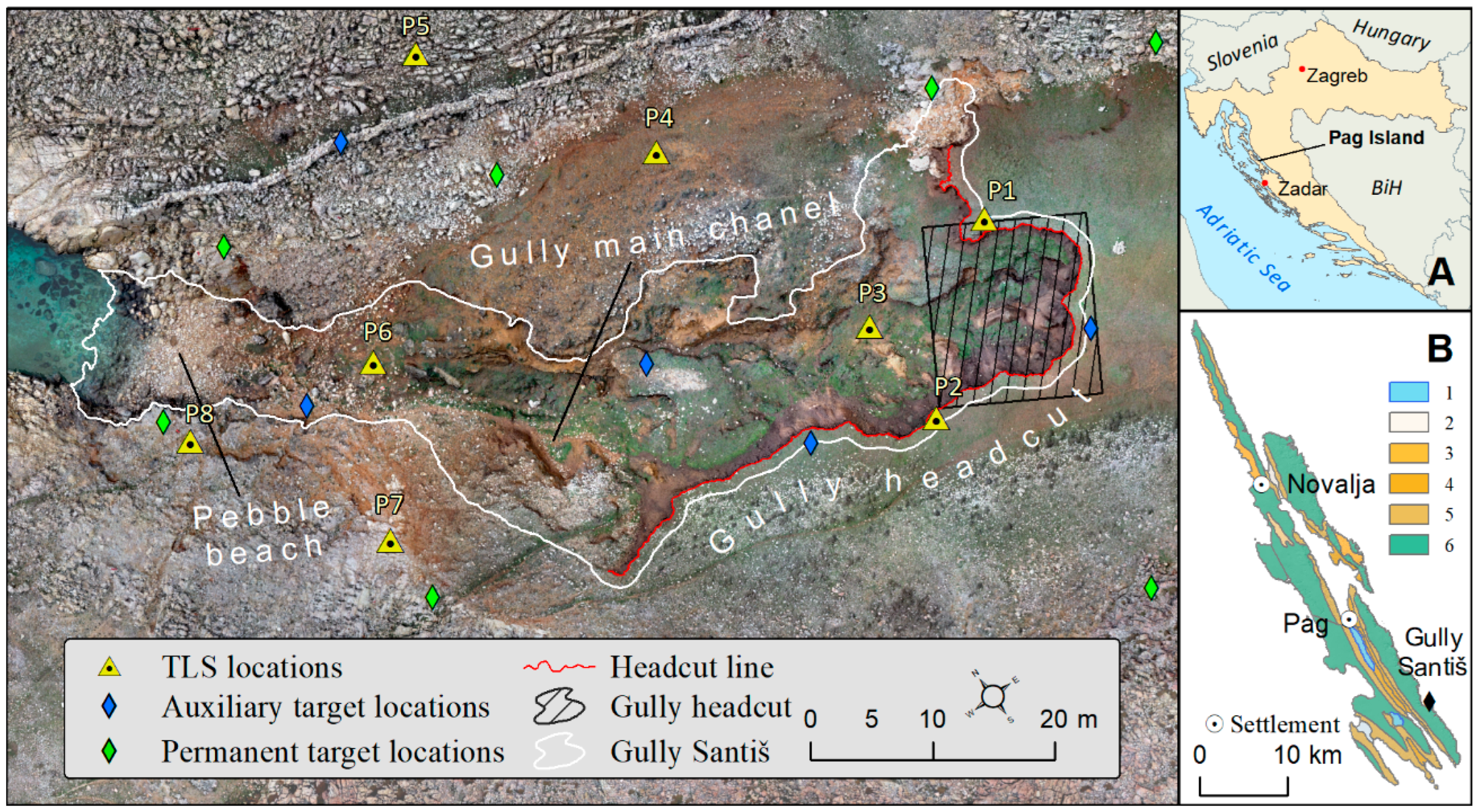
2.1. Study Area

The developed framework was tested on a gully Santiš, located on the SE part of Pag Island, Croatia (Figure 1A,B). Pag Island is known for harsh climatic conditions and absence of vegetation cover that have led to the formation of numerous gullies and other erosional forms [42,43,44]. According to [44], more than 30% of the whole island is characterized by high susceptibility to gully erosion. Mean annual precipitation at Pag Island is 977.5 mm and mean air temperature is 15.5 °C, with pronounced seasonal heterogeneity, expressed through variations between very hot and dry summers and rainy springs and autumns [43].
Gully Santiš was chosen as the perfect site for testing and validation of the developed framework, due to its complex morphology and rapid soil erosion induced STCs. Gully Santiš was formed predominantly by water erosion in Kalkocambisol soil sediments a few meters deep, which are surrounded and underlined by limestone and dolomite carbonate rocks [43]. The dominant erosion type within gully Santiš is rainfall induced erosion, which causes an annual gully headcut retreat up to 24.85 ± 5 cm year−1 [43]. Although gully Santiš is relatively short (80 m), its morphology comprises an imposing, gully headcut over 140 m wide and a few meters deep, from which a single deeply incised channel leads to a pebble beach at the contact with the Adriatic Sea (Figure 1). The gully headcut is characterized by steep sides and overhangs, formed by gradual material mass collapse and uphill headcut retreat. Such complex morphology represents a challenge for non-systematic multi-temporal terrestrial LiDAR surveys, as the probability for occurrence of obstructed areas is very high.
The second challenge posed for the performance of multi-temporal terrestrial LiDAR surveys over gully Santiš is the rapidity of STCs, which are constantly changing the shape of the gully, thus raising the probability for occurrence of obstructed areas. Rapid erosion induced STCs within gully Santiš are mainly occurring within the initial parts of the gully, due to the gradual collapse and uphill progression of the gully headcut [43].
The study area within this research can be divided into two separate sub-areas, where different research goals were implemented. The first study area (SA-1) covers the whole gully Santiš (1226.97 m2), where the main goal was to test the performance of the developed framework for TLS survey optimization. Within this larger area, only the first field LiDAR survey was conducted, as this was enough to validate the performance of the actual field TLS survey over the planned outcome.
The second sub-area (SA-2) covers the chosen part of the gully headcut (199.23 m2), where the most intensive traces of headcut uphill regression were noted during the previous field research [43]. For this sub-area, two TLS surveys were conducted, which allowed for (a) validation of the performance of multi-temporal TLS surveys and (b) detection and quantification of spatio-temporal changes.

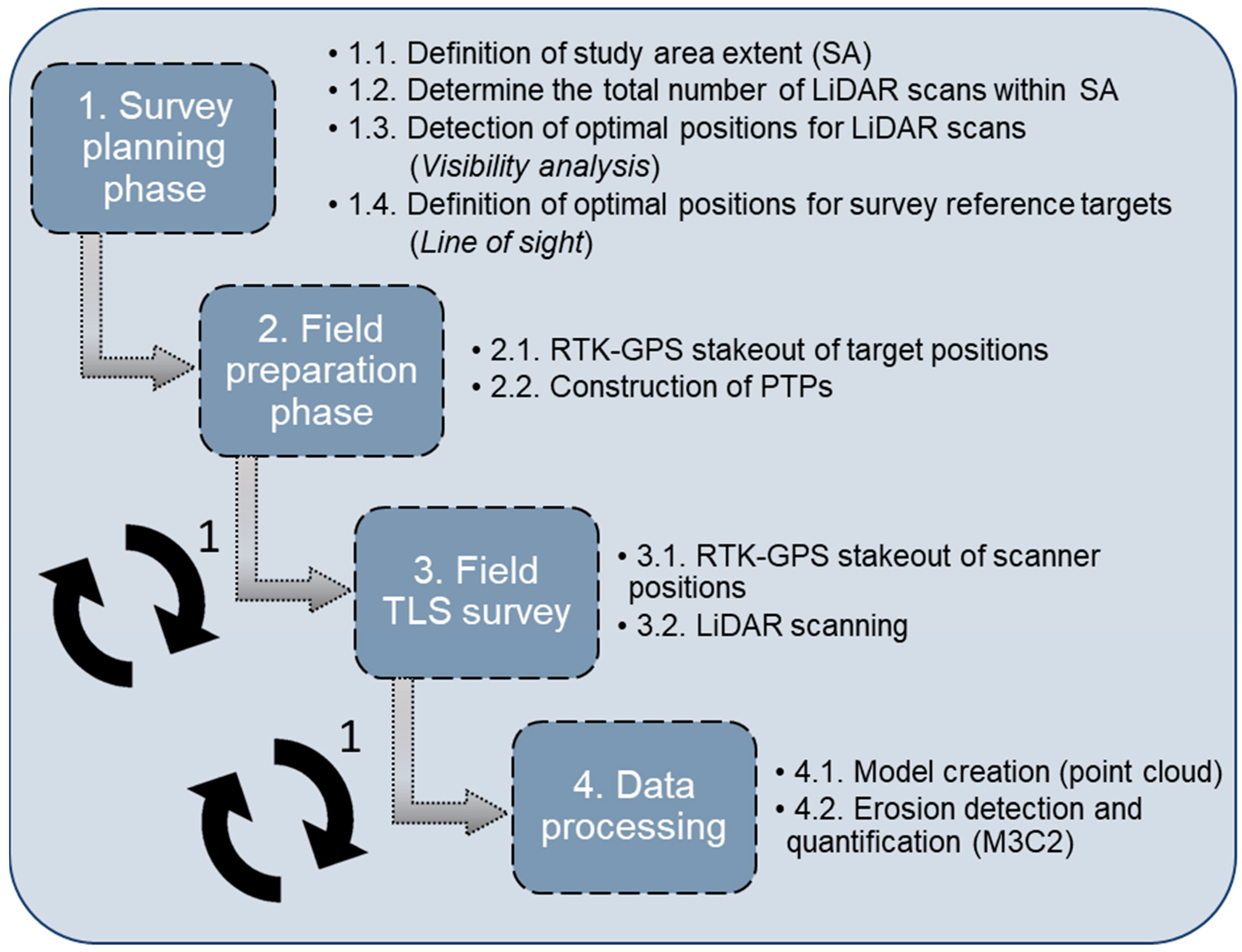
2.2. Systematic Optimization of Multi-Temporal TLS Surveys

The developed methodology for systematic optimization of multi-temporal TLS surveys can be divided into following four main phases: (1) survey planning, (2) filed preparation, (3) multi-temporal field TLS surveys and (4) data processing (Figure 2).
  • Survey planning phase
The survey planning phase is the most important phase of the whole developed systematic framework, which determines the basic characteristics of multi-temporal TLS surveys. According to [45], TLS surveys should: (1) have several TLS positions aimed at the target surface, (2) assure significant overlap between different scans and (3) use at least four fixed targets for each scan. Therefore, the developed systematic framework considers these recommendations during the survey planning phase.
The initial step in the planning phase is definition of study area extent (1.1.), thus determining within which area will multi-temporal surveys be applied. Considering that the study area within this research covered the whole extent of gully Santiš (SA-1) and the chosen part of the gully headcut (SA-2), both these areas had to be completely included in the defined study area extent. The second step of the planning phase is determination of the total number of LiDAR scans within the study area (1.2.), through which the user has to determine the optimal number of LiDAR scans, considering the (a) available survey duration and (b) characteristics of the available terrestrial laser scanner. Within this research, it was planned that each LiDAR survey would last between 3 and 5 h, where every scan would optimally last around 30 min. Therefore, the total number of LiDAR scans was set to eight scans. In order to stay within a 30 min range per scan, characteristics of LiDAR scanning had to be adjusted accordingly. Within this research, a Faro Focus M70 terrestrial laser scanner was used, while scanning parameters were set to: resolution = ½; quality = 3× (Figure 3A). Parameter ½ resolution controls the density of the point cloud, while parameter 3× quality controls the accuracy of collected measurements. Faro Focus M70 TLS has a range between 0.6 m and 70 m, along with a measurement speed of up to 488,000 points/second, a wide scanning angle (360° horizontal and 300° vertical view) and a ranging error of ±1 mm at around 25 m [46].
Once the total number of survey scans is determined and scanning parameters are set, the next step is to find optimal TLS positions (1.3.) within and around the chosen study area, from which it is possible to achieve the greatest coverage of the whole study area. Determination of these optimal TLS positions is done through viewshed analysis, which is automated within this research by the newly developed, open-source TLS positioning tool (TPT). The TPT allows simultaneous verification of multiple (up to several hundred) selected potential TLS positions, where total coverage of study area and scan overlap are calculated for every tested position. All positions with coverage value under the user defined threshold (e.g., 75%) could be automatically removed by the TPT from further consideration. Furthermore, within the TPT, users can adjust parameters of visibility analysis (OFFSETA, OFFSETB, VERT1, VERT2, RADIUS1 and RADIUS2 [47], according to the characteristics of the TLS survey and specifications of the terrestrial laser scanner (e.g., Faro Focus M70). Spherical and atmospheric errors can in some cases significantly influence the results of viewshed analysis [46,47,48,49], thus adjustments of Earth curvature correction and refraction coefficient have been allowed optionally within the TPT.
Viewshed analysis performed by the TPT requires a high resolution digital surface model (DSM) of the chosen study area, serving as a basis for determination of coverage with laser beams from every tested TLS position. A schematic representation of the TPT, created in the Model Builder extension of the ArcGIS 10.1 software is given in Supplementary Figure S1.
Within this research, the TPT was used for determination of eight optimal TLS positions, among the more than 100 potential TLS positions scattered within and around the gully Santiš. An existing very-high resolution (VHR) DSM with 1.9 cm spatial resolution created by UAV photogrammetry within earlier research [43] was used as an input VHR DSM for visibility analysis and selection of eight optimal TLS positions. Within this study, parameters of viewshed analysis were adjusted to the specifications of the Faro Focus M70; thus, height of TLS (OFFSETA) was set to 1.9 m, scanner vertical view was set to 90° (upper vertical scanning angle—VERT1) and −65° (lower vertical scanning angle—VERT2), while the scanner range was set between 0.6 (RADIUS1) and 70 m (RADIUS2) (Supplementary Figure S1). Height of target areas (OFFSETB) was set to 0 m, as it was planned that the TLS survey would cover the terrain surface. As the study area covered a relatively small area, spherical and atmospheric errors were not accounted for. From all tested potential TLS positions, the eight locations with the highest overlap and areal coverage were determined as optimal scanning locations. An example of coverage planned for the first optimal TLS position is given in Figure 4.
The final step of the survey planning phase is definition of optimal positions for survey reference targets (1.4.), which are required for accurate registration of multiple surveyed scans and relative orientation of multi-temporal surveys. As such, these targets have to be placed on exact XYZ locations, which will be identical for every multi-temporal TLS survey and will not be affected by ongoing erosion processes. Due to that, the optimal locations for reference targets within this study had to be placed within surrounding carbonate rocks, outside of the soil material affected by gully erosion. Furthermore, in order for reference targets to be visible from as many TLS positions as possible within the rough gully terrain, they had to be placed on specially designed metal poles at the height of 210 cm (Figure 3B). After selection of potential optimal locations within and around the gully, visibility of every chosen target from defined eight TLS positions was validated by the Line of sight tool (Figure 4B). In total, seven optimal locations for reference targets were chosen and validated with the Line of sight tool, while it was assured that at least four reference targets were visible from every TLS position at a distance under 35 m. In order to avoid scattering of points at the reference target, the distance between TLS position and reference targets was never above 35 m, as recommended in the specifications of the Faro Focus M70 [46]. These seven locations served as a basis for creation of permanent target positions (PTPs) within the field preparation phase.
2.
Field preparation phase
The second phase within the developed systematic framework covers all activities related to the field preparations for later multi-temporal LiDAR surveys. The first activity included GPS stakeout of target positions (2.1), where all seven chosen optimal locations for reference targets were staked out in the field using the Trimble R12i GNSS system. At every stakeout location, there followed construction of permanent target positions (2.2.), which included carving of permanent stands for metal poles in carbonate bedrock with a hammer drill (Figure 5A) and leveling of permanent target positions with self-leveling concrete (Figure 5B). This resulted in a solid flat surface on which metal poles were anchored using four steel anchors (① in Figure 5B). Such a design allows fast and accurate installation of permanent targets (spheres) at chosen locations before every multi-temporal TLS survey. In order to protect steel anchors from corrosion in-between multi-temporal LiDAR surveys, plastic cover (② and ③ in Figure 5B) was placed on top of anchors. Seven 2.1 m long metal poles were then used to fix reference targets above constructed PTPs (Figure 5B,D,E). Metal poles can be dissembled and stored in between two LiDAR surveys, while constructed PTPs are then protected from long-term exposure to weather and corrosion by nylon and gypsum protective caps (Figure 5C). Finally, before every LiDAR survey, reference target spheres (d = 69.5 cm) (① in Figure 5D) were placed on designed metal poles (② in Figure 5D), which were earlier installed on constructed PTPs (③ in Figure 5D).
3.
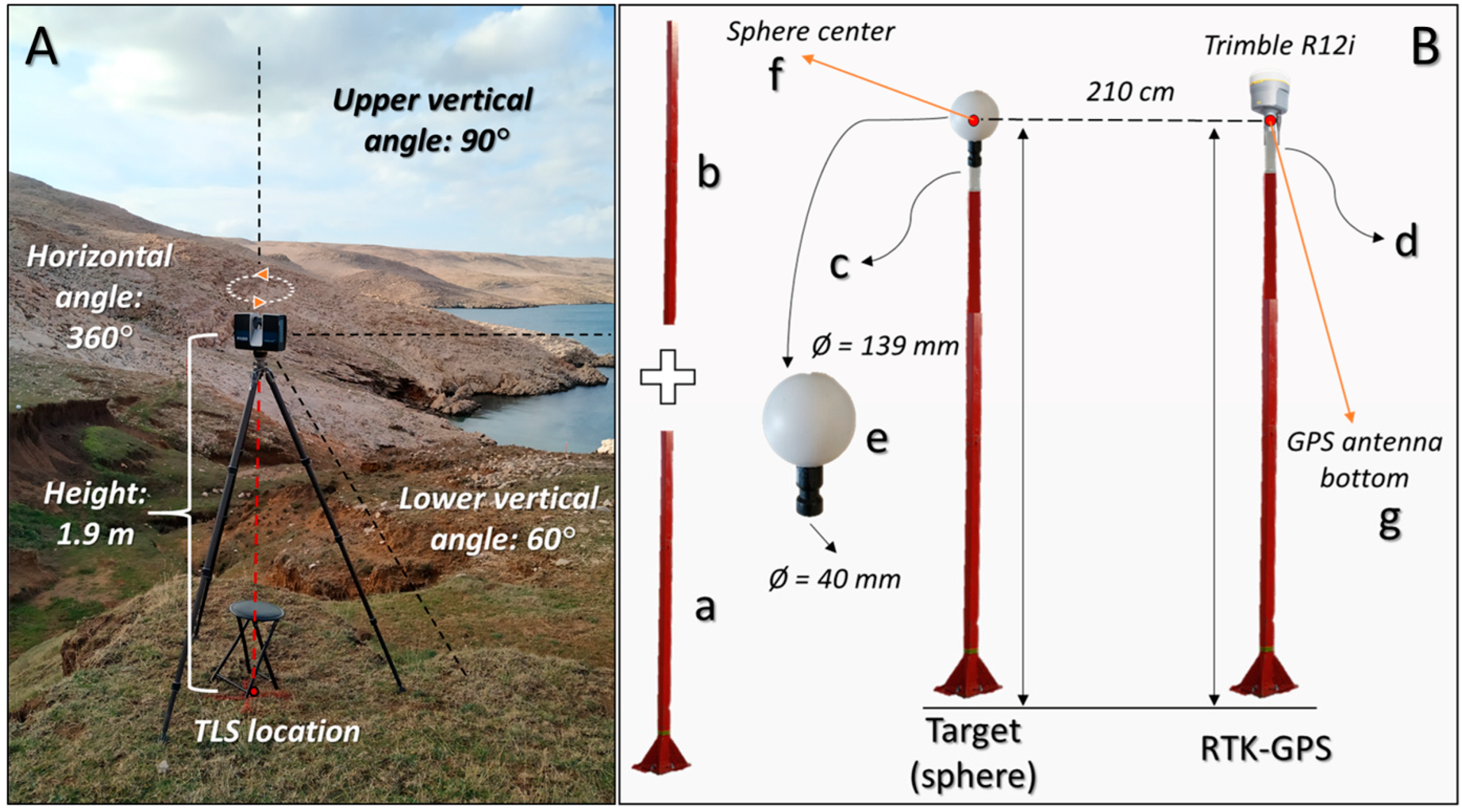
Multi-temporal field LiDAR surveys
The third phase of the developed systematic framework covers multi-temporal field TLS surveys. The first activity included field stakeout of TLS positions (3.1.), which were staked out separately before every multi-temporal LiDAR survey using the Trimble R12i GNSS system. As most TLS positions were within loose soil material, permanent position marks have not been used. Instead, every TLS position was marked with red spray just before the field LiDAR survey. Prior to every field LiDAR survey, all seven standard reference targets (d = 69.5 cm) were placed on metal poles anchored to the constructed PTPs, while additional auxiliary targets were placed in-between (Figure 1). Precise coordinates of every sphere, placed on top of a metal pole with a specially designed mount (Figure 3B) was collected before the initial survey with 50-epoch RTK positioning using the Trimble R12i GNSS system. Coordinates of every reference target (sphere) collected with 50-epoch measurements are given in Supplementary Table S1.
The second step of this phase covers the actual multi-temporal field LiDAR survey (3.2.). For each multi-temporal survey, a Faro M70 TLS mounted on a carbon tripod was used to scan the selected study areas (SA-1 and SA-2) from defined optimal TLS positions. The initial LiDAR survey of the chosen gully site was conducted on 17 December, 2019, while the final LiDAR survey was conducted on 17 December, 2020. While the initial LiDAR survey covered the whole study area (SA-1), where scanning was performed from all eight planned TLS positions, the second LiDAR survey covered only the chosen part of the gully headcut (SA-2), which was covered from the first five planned TLS positions. The second TLS survey was limited only to SA-2, as it was decided that analysis of soil erosion induced STCs would be performed just within this area with the most distinctive traces of recent active soil erosion.
4.
Data processing and model creation
The last phase of the developed framework covers data processing and model creation (4.1.) and detection of STCs (4.2.). The identical methodology for processing of collected LiDAR scans and creation of VHR models was used for data collected by both TLS surveys. A detailed graphical representation of the whole data processing and VHR model creation is given in Figure 6.
Collected scans of each TLS survey were processed as individual projects in Faro Scene software, which allowed processing and registration of collected scans, as well as creation of a point cloud representing the whole study site. All collected LiDAR scans of TLS surveys were added to the Faro SCENE, and processed using the user-defined parameters described in Figure 6. In order to remove points with a high error, collected scans were filtered using the following filters: Dark Scan Point Filter, Stray Point Filter and Edge Artefact Filter. Additionally, since standardized reference targets were used during the field TLS survey, the automatic detection option was enabled for detection of spheres with active radii of 69.5 cm.
The second part of LiDAR scan processing was related to the automatic registration of processed individual scans, using the target-based registration approach (Figure 6). Before automatic registration, all detected targets were manually verified, whereby all falsely detected targets (e.g., boulders and similar round objects) were manually removed. After manual verification, names of remaining targets were assigned (T1–T7). Automatic registration was performed using the forced correspondence by target names (Figure 6). At the end of the registration process, precise target (sphere) coordinates, collected during the field preparation phase with RTK-GNSS, were added to each sphere, thus allowing final absolute georeferencing and automatic registration of the created LiDAR cluster. The mean TLS survey error was calculated for each survey based on the mean vertical and horizontal errors, as well as the mean distance error.
The final step of the methodology applied for processing of multi-temporal LiDAR data covered automated creation of point clouds from the registered cluster (Figure 6). Finally, the created point cloud for each TLS survey was exported so that it could be used for later processing and analysis.

2.3. Validation of Performance of Developed Framework in Comparison to Non-Systematic TLS Survey Approach

Validation of the performance and successfulness of the developed framework for systematic optimization of multi-temporal TLS surveys was based on comparison of achieved coverage with the coverage achieved by the traditional, non-systematic TLS survey. This non-systematic TLS survey was carried out over the identical study area in March 2017 using the Stonex X300 TLS (Figure 7A). A non-systematic TLS survey with Stonex X300 TLS was carried out from seven different TLS positions within and around gully Santiš (Figure 7B) where the main goal was to achieve the highest possible coverage over the gully headcut. Optimal TLS positions for the non-systematic survey were determined on site without any prior planning. Thus, selection of seven optimal TLS positions was based entirely on terrain characteristics and user experience and judgment. TLS positions were placed on flat locations within and around gully Santiš, for which it was estimated that they should provide the best visibility of surrounding gully morphology. In-situ determination of optimal TLS positions was very demanding, as complex gully morphology and size of study area presented serious challenges during the selection of seven optimal locations.
In order to achieve highest possible point cloud density, fine resolution scanning mode was set for all seven TLS positions. Within fine resolution scanning mode, each scan with Stonex X300 TLS lasts around 53 min, where about 64,000,000 points are collected (Stonex, 2022). Collected scans were registered by standard reference spheres (d = 69.5 cm) that were scattered throughout the study area prior to the survey.

2.4. Detection of Spatio-Temporal Changes within Gully Headcut

Detection of soil erosion induced STCs was performed within the CloudCompare software (v2.6.1.), using the Multiscale Model to Model Cloud Comparison (M3C2) algorithm. The M3C2 algorithm was already successfully applied for point cloud-based detection of STCs caused by various geomorphic processes, such as river dynamics [50], soil erosion [27,51,52,53], rockfalls [12,54], rock glaciers [54,55,56], etc. Since the M3C2 algorithm is a point cloud-based method, it allows detection of complex (3D) soil erosion induced STCs, thus successfully overcoming the shortcomings of DEMs of difference (DoDs) related to the complex morphology of erosional forms [51,52,57]. As DoD represents a 2.5D model, significant errors can occur during the detection of STCs, especially in complex steep and overhanging parts of the terrain where 2.5D models cannot accurately represent the terrain morphology [50,58,59,60].
The M3C2 algorithm calculates the distance between two point clouds with an assessment of the reliability of the calculated distance based on terrain complexity and registration error [57,61,62,63]. Distance between point clouds is calculated within the cylinder of a user-defined radius (d/2) that is projected along the normal (N) of each point (i) of the initial point cloud [57,62]. When applying the M3C2 algorithm, user-defined parameters should be taken into account, as these can greatly affect the output results [12,51,60]. The most important user-defined parameter within the M3C2 algorithm is radius of the normal (D/2) [60], as the increase in its value is directly reflected in the lowering of influence of local fragmentation and terrain complexity on distance calculations, thus leading to the generalization of calculated M3C2 distances [51,60]. From user-defined parameters, radius of the normal (D/2) was set to 10 cm, cylinder radius (d/2) was set to 20 cm, while max depth was set to 1.5 m. Preferred orientation was set to +Z and registration error was set to 1.33 cm This registration error was calculated as average of the mean TLS survey errors of two conducted TLS surveys.
In order to calculate volumetric STCs which have occurred within the observed one-year period, point clouds were interpolated in the CloudCompare software using the Kriging interpolation method with a grid spacing of 5 mm. Detection of volumetric STCs was performed in ArcGIS 10.1 software, using the Geomorphic Change Detection 7 add-on [64,65,66]. During the detection of volumetric STCs, GDC7 considers the uncertainty of multi-temporal models, which is taken as the minimal level of detection [51,67]. The minimal level of detection threshold ( L o D m i n ) was set accordingly to the mean TLS survey error, which was 1.29 cm for TLS survey 2019, and 1.37 cm for TLS survey 2020, with 0.95 confidence level probabilistic thresholding applied.

3. Results

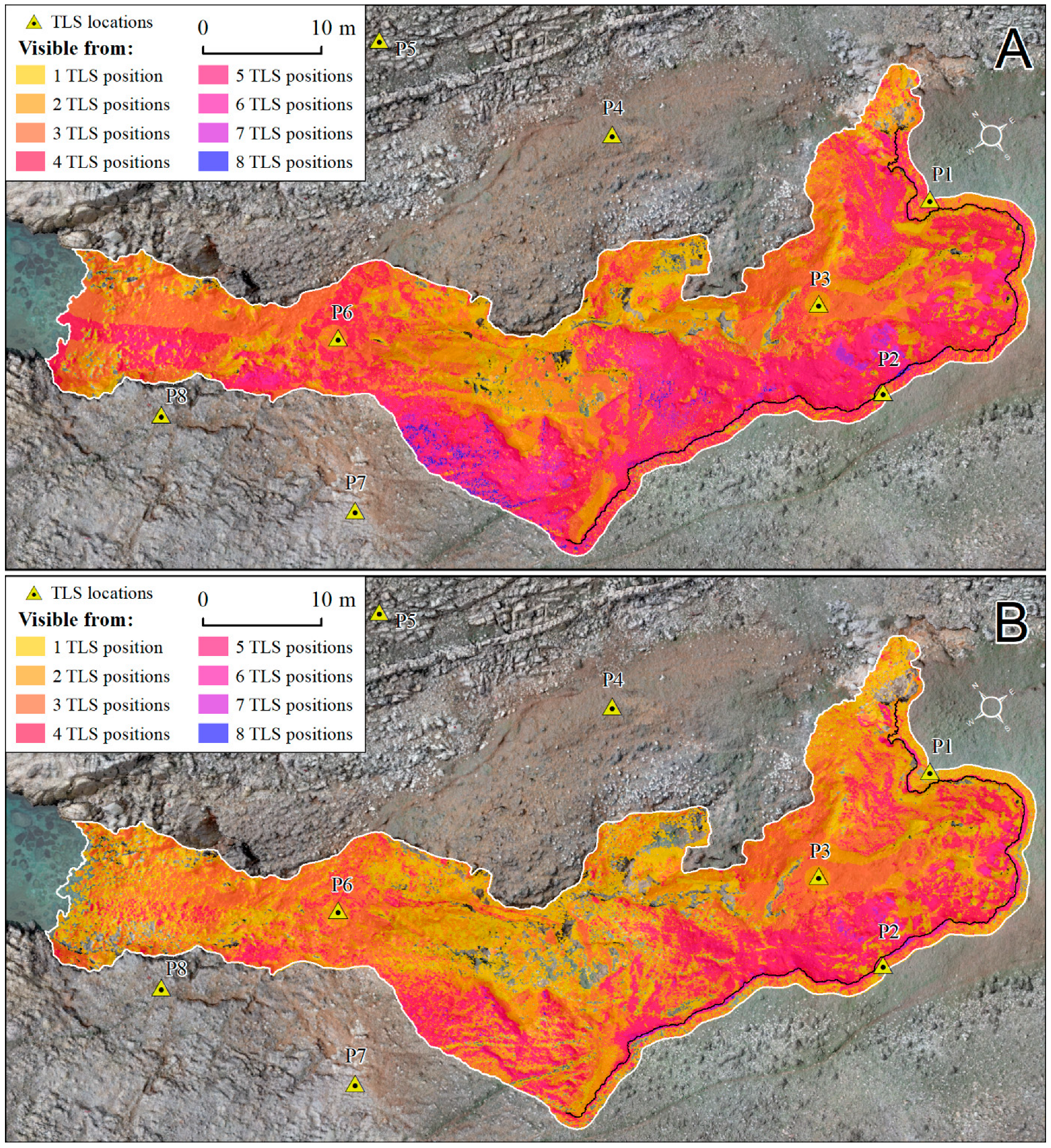
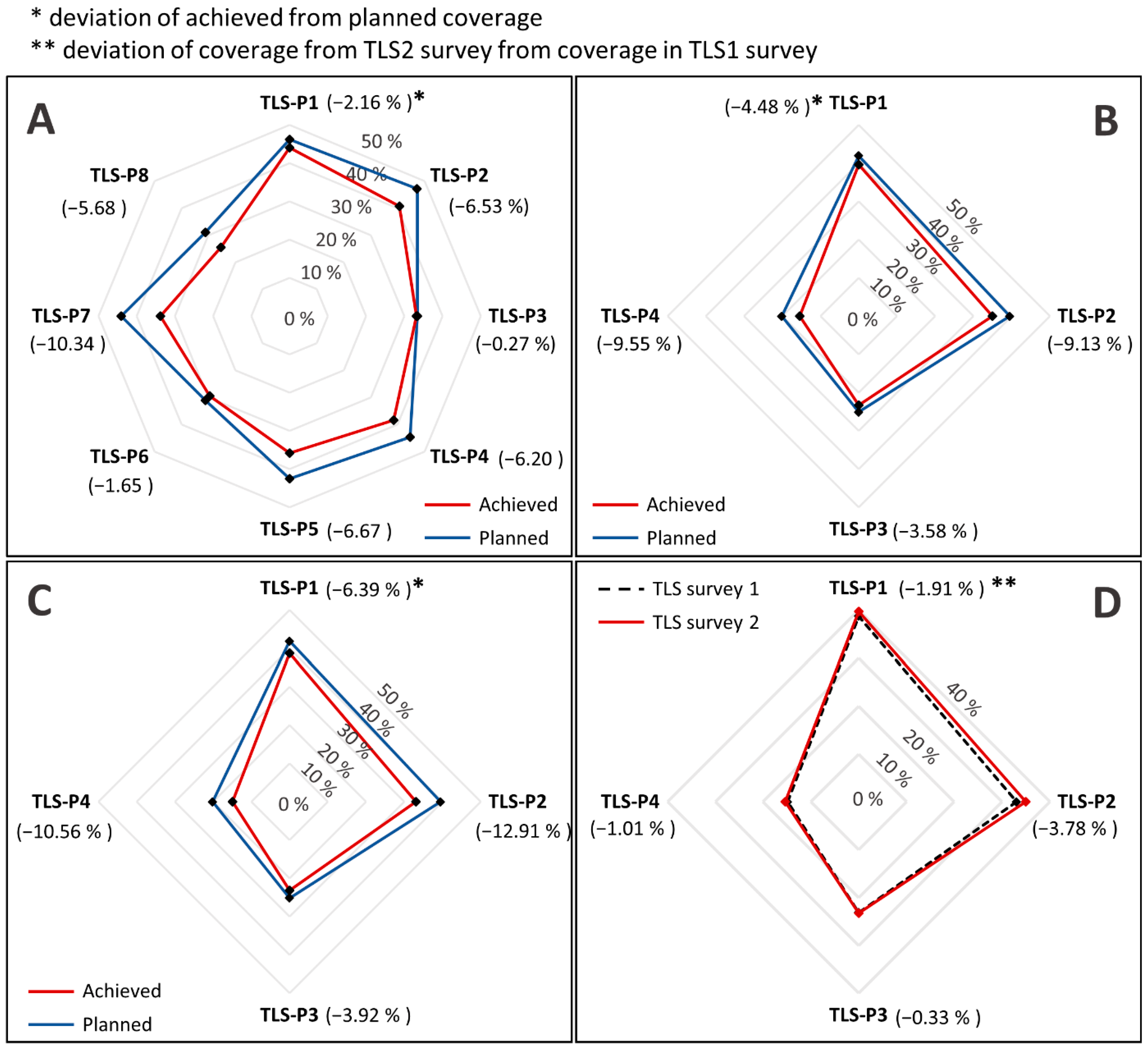
3.1. Comparison between Planned and Achieved Coverage of Study Area with Optimized TLS Surveys

From more than 100 potential TLS positions that were considered for placement of TLS within the chosen study area by the TPT, eight optimal TLS positions were chosen (Figure 1), allowing the very-high percentage of planned coverage. Despite the complex morphology of gully Santiš, performed optimization has shown that almost 97% (1190.04 m2) of the whole SA-1 area should be covered by multi-temporal TLS surveys from those eight optimal chosen TLS positions (Table 1). According to the developed multi-temporal TLS survey plan, obstructed areas cover only 3.1% (36.93 m2) of the whole gully Santiš and are not visible at all from any of the eight chosen TLS positions.
If SA-2 is considered, then percentage of planned coverage is even higher, accounting for up to 97.12% (193.49 m2) of total study area (Table 1). It should be noted that within SA-2, overlap between different neighboring TLS positions is very high, thus significantly increasing the overall density of collected points.
In order to validate the performance of the whole optimization process, planned coverage was compared to the results of actual multi-temporal field TLS surveys. While within SA-1 planned coverage was compared to the results of the initial TLS survey (TLS survey 2019), within SA-2 planned coverage was compared to both the initial (TLS survey 2019) and second multi-temporal TLS survey (TLS survey 2020).
Final point clouds created from carried out multi-temporal TLS surveys are visible in Figure 8. The point cloud for SA-1 created from scans collected within the initial TLS survey has in total 137,240,252 points, with average point density of 88,428 points per m2 (Figure 8A). Point clouds for SA-2 have 25,875,206 (TLS survey 2019—Figure 8B) and 26,650,29 (TLS survey 2020—Figure 8C) points, with average point densities of 92,411.45 and 95,179.63 points per m2, respectively. The highest point density in both TLS surveys is in the initial part of the gully, where the highest overlap from chosen TLS positions was achieved.
Both multi-temporal TLS surveys have confirmed the accuracy and excellent performance of the carried out optimization, with minimal deviations of the achieved TLS survey coverage from the planned coverage in both SA-1 and SA-2.
In total, the initial TLS survey covered 1181.07 m2 of SA-1 (96.26% of the total study area), which deviates from planned coverage for only 8.97 m2, or 0.73% (Table 2). The highest concentration of obstructed areas was in the middle part of the gully, within the deeply incised sub-channels of the main gully channel (Figure 9B).
However, these obstructed areas are also present to a lesser extent at exactly the same locations in the planned coverage (Figure 9A), thus confirming the congruence of the planned survey with actual results of the field TLS survey (Figure 9B).
It should be noted that achieved coverage from individual TLS positions for SA-1 is slightly lower than the corresponding planned coverage (Table 2; Figure 10A). On average, achieved coverage from each individual TLS position was lower by 4.93% than the planned coverage, while for some TLS positions, achieved coverage was even significantly lower (e.g., TLS position 7—10.34% (Figure 10A)). The highest deviation was recorded at TLS positions that were either within very steep and complex terrain (P2; P8; P7), or that were considerably distanced from SA-1 (P5) (Figure 9A). The smallest deviation (0.27%) of achieved coverage from planned was recorded in the third TLS position (P3), located on the flat area in the central part of the gully channel. Deviation of planned and achieved coverage within SA-1 for each individual TLS position is represented in Figure 10A. Although achieved coverage from individual TLS positions was lower than planned, carried out optimization allowed significant scan overlap that compensated for lower coverage of individual scans and allowed achievement of excellent total coverage for the whole SA-1 area.
Furthermore, achieved scan overlap from eight chosen TLS positions (Figure 9A) for the initial TLS survey was also lower than planned overlap (Figure 9B), especially in terms of areas covered from three or more TLS positions (Supplementary Table S2). While in planned coverage about 69% of SA-1 should be covered with overlapping scans from three or more TLS positions, within achieved coverage only 48% of SA-1 was covered from three or more TLS positions. This is especially evident with overlap achieved from six or more TLS positions, which is significantly less represented within the achieved coverage (Figure 9B).
Within SA-2, both carried out TLS surveys confirmed the performance of carried out systematic optimization and created survey plans, with very-high rates of achieved coverage (Table 3). Deviation of achieved from planned coverage within SA-2 is slightly higher than in SA-1, with an increase of deviation from the initial TLS survey up to the second survey. While achieved coverage for initial TLS survey covered 195.70 m2 (98.23% of the total study area), the second TLS survey covered 193.49 m2 (97.12% of the total study area). As seen in Table 3, due to the obstructed areas, the initial TLS survey deviates from planned coverage for 1.87%, while the second TLS survey deviates for 2.98%. As in SA-1, these obstructed areas are related to complex overhangs of gully headcut and deeply incised sub-channels at the bottom of the headcut (Figure 9B).
A gradual increase in the deviation of achieved from planned coverage within performed multi-temporal TLS surveys is also evident within the individual TLS positions of each carried out survey (Figure 10B,C). It is noticeable that deviations increased at all four TLS positions within SA-1 between two multi-temporal TLS surveys (Figure 10D). However, the increase in deviation was not uniform for all TLS positions. Identically as in SA-1, the smallest deviation within SA-2 was recorded within P3 (−0.33%), while the increase was larger for the other three positions. As in SA-1, the deviation was highest for both carried out TLS surveys within P2 (−3.78%), where due to the rapid retreat rate of the gully headcut, it was not possible to place TLS at a completely identical location. Due to intensive STCs in the TLS-2020 survey, TLS postion P2 had to be shifted from its original position by less than 5 cm. This confirms that even the smallest deviation in placement of TLS from the planned position could lead to the significant lowering of the achieved coverage. Overall, carried out multi-temporal TLS surveys have confirmed the accuracy, reliability and repeatability of the developed new systematic framework.

3.2. Comparison with Coverage Achieved through the Non-Systematic TLS Survey Approach

Further validation of the success of the developed framework was carried out through comparison of achieved coverage to the coverage achieved through the traditional non-systematic TLS survey approach. A non-systematic survey carried out in 2017 with a Stonex X300 resulted in a point cloud with 443,572,261 points, from which about 75% are outside the study area (SA-1). In total, 110,893,065 points from the created non-systematic point cloud are within SA-1. The mean TLS survey error for the non-systematic survey was 3.14 cm, mainly due to the obstructed reference targets and distance between chosen TLS stations.
Overall, non-systematic TLS surveys have not managed to achieve the level of coverage that was achieved through the developed systematic framework. In total, the carried out non-systematic TLS survey covered 1047.39 m2 of SA-1 (85.36% of the total SA-1 study area), which deviates from the coverage achieved by the initial planned TLS survey (TLS survey 1) by 133.68 m2. The non-systematic survey approach covered about 10.9% less of the SA-1 study area than the initial systematic TLS survey, thus confirming the successful performance of the developed systematic framework.
Results are similar within SA-2, where coverage achieved through the non-systematic survey approach is slightly better, mostly due to the higher overlap between the first four TLS scanning positions of the carried out survey. In total, the carried out non-systematic TLS survey covered 174.31 m2 of SA-2 (87.49% of the total SA-2 study area), which deviates from the coverage of the initial planned TLS survey (TLS survey 1) by 21.39 m2, and from the coverage of the second planned TLS survey (TLS survey 2) by 19.18 m2. Thus, the non-systematic TLS survey covered about 10.8% less of the SA-2 study area than TLS survey 1, and 9.63% less of the SA-2 study area than TLS survey 2.

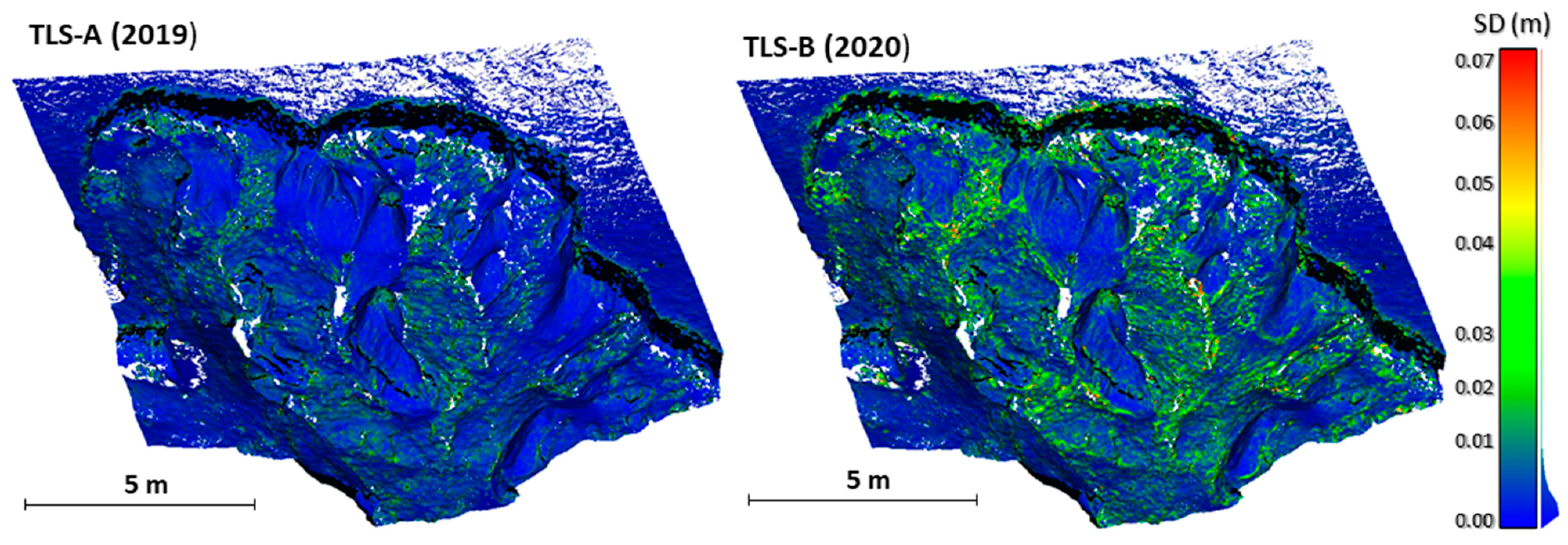
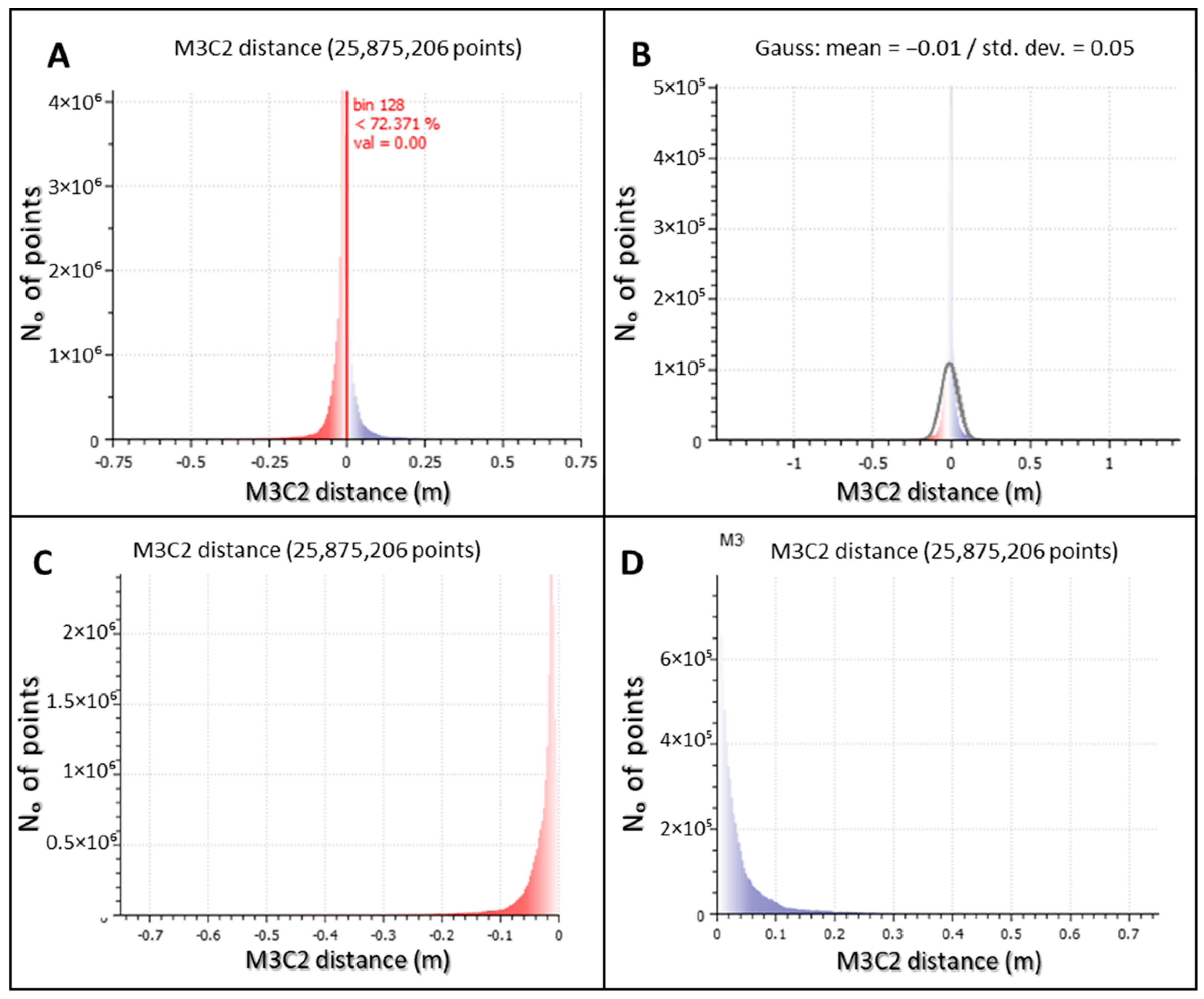
3.3. Detected Spatio-Temporal Changes within Gully Headcut (SA-2)

Point clouds of SA-2 created within carried out multi-temporal TLS surveys were used for detection of soil erosion induced spatio-temporal changes that have occurred within a one-year period. Table 4 presents the basic characteristics of point clouds used for detection of spatio-temporal changes by the M3C2 algorithm, while point clouds can be seen at Figure 8B,C. The mean TLS survey error was 1.29 cm for theTLS-2019 survey and 1.37 cm for the TLS-2020 survey.
While total number of points in each point cloud and average point density are similar between the two TLS surveys, standard deviations (SDs) of each point cloud calculated by the M3C2 algorithm are very disparate (Figure 11). Standard deviations of the initial TLS survey are much lower, with maximal values up to 2.5 cm. On the other hand, SDs of the second TLS survey are much higher, with maximal values ranging up to 7 cm. Such high SD values in the second TLS survey were caused primarily by soil erosion induced spatio-temporal changes that have occurred within the observed one-year period. The spatial distribution of higher values of the SD in the point cloud of the final TLS survey indicates where most intensive STCs have occurred. Most of these high SD values are concentrated along the edge of gully headcut, especially at locations where mass wasting of material from the edge of gully headcut has occurred within the observed one-year period. Furthermore, higher SD values are noticeable in the first few meters below the gully headcut, where material eroded from the headcut was gradually accumulated. Detected accumulation is mostly located along the rills formed in loose material within the gully. Although SD values could indicate where STCs have occurred, they do not allow differentiation of negative from positive STCs. Therefore, better representation of STCs is given by calculated M3C2 distances (Figure 12 and Figure 13).
Calculated M3C2 distances indicate that within the observed one-year period, erosion prevailed within SA-2, with negative distances accounting for 72.31% of all measured distances (Figure 12A). Predominance of erosion is further confirmed with the Gaussian distribution of all STCs detected by the M3C2 algorithm, where the mean Gaussian value for the observed period was −1 cm (Figure 12B). Both erosion (Figure 12C) and accumulation (Figure 12D) related M3C2 distances are mostly under 10 cm, thus indicating that in most cases STCs occurring between December 2019 and December 2020 were of low intensity. Although higher M3C2 distances are far less represented, their importance for understanding and interpretation of overall evolution of SA-2 is very high. While the highest negative M3C2 distances range in some cases over 75 cm, highest positive M3C2 values range at some points up to 20 cm.
During the study period between December 2019 and December 2020, a total of 2.42 m2 of sediment was generated within SA-2, where 1.73 m2 of that eroded material was accumulated within the study area, while only 0.69 m2 (28.59% of eroded material) was transported further from the headcut, outside of SA-2.

4. Discussion

4.1. Advantages of the Developed Framework over the Non-Systematic TLS Survey Approach

Carried out systematic TLS survey optimization and performed visibility analysis resulted in excellent performance for both carried multi-temporal TLS surveys, especially in regard to the high percentage of achieved coverage over the complex gully morphology. Obstructed areas that are present in created point clouds are mainly restricted to hidden parts at the bottom of steep and incised sub-channels within the main gully channel or to smaller areas within deeper overhangs in the gully headcut. However, if total gully size and complexity are considered, the presence of these obstructed areas is negligible.
On the other hand, the presence of obstructed areas in the point cloud created through the non-systematic approach is significantly higher, especially in areas of complex morphology. Visual comparison of the presence of obstructed areas within identical parts of the gully headcut in the point cloud created by the non-systematic approach (A) and in the point cloud created by the developed systematic framework (B) is visible in Figure 14. In some parts of the gully headcut, the presence of obstructed areas within non-systematic survey is so high that it was not possible to use this data for detection of STCs. Similar problems with the high presence of obstructed areas within point clouds created through non-systematic approaches were reported in a lot of other research. For example, obstructed areas were reported at the gully bottoms [23,26] or at the incised parts of the gully [26,32,40]. The presence of obstructed areas in non-systematic surveys is mostly related to the larger and more complex erosional forms (e.g., gullies and badlands), while smaller forms (e.g., rills and ephermal gullies) are less frequently affected by such areas [36].
Furthermore, lower performance of non-systematic surveys can be seen in higher values of the mean TLS survey error, which is significantly higher for the non-systematic survey than it is within both carried systematic multi-temporal surveys. A combination of higher distances between certain TLS positions, lower scan overlap and higher presence of obstructed areas presented a challenge for registration of seven collected scans, which led to the overall increase in mean TLS survey error of the non-systematic survey. Such higher survey errors influence the accuracy of created point clouds and raises the minimal level of detection, thus lowering the probability of detecting important small scale erosion induced STCs from created point clouds.
It should be noted that Stonex X300 has slightly different specifications than Faro Focus M70, especially in regard to longer operational range (up to 300 m), smaller vertical scanning angle (−25°–65°) and lower point density (up to 60,000 points/s) (Stonex, 2022). These specifications are less optimal for scanning of complex gully morphology, in comparison to specifications of Faro Focus M70, especially in regard to less favorable vertical scanning angle. The lower vertical angle of Stonex X300 prevents the scanning of complex overhangs and other rough areas in close vicinity to the scanner position, thus contributing to the overall lower achieved coverage of the non-systematic survey.
Overall, it should be noted that the developed systematic TLS survey framework significantly improved the repeatability and accuracy of multi-temporal TLS surveys over complex gully morphology, especially in terms of achieved coverage of the study area and lower mean TLS survey error. The main novelty of the developed framework is the implementation of the survey planning and filed preparation phases before the actual field TLS survey, which used visibility analysis and the developed TLS positioning tool (TPT) for selection of optimal TLS survey stations and optimal reference target locations. This ensures not only that TLS will be placed on locations that will allow best-possible coverage of a certain study area, but also that all TLS survey stations and reference target locations will be identical within all carried out multi-temporal TLS surveys. Since in most cases, optimal locations of TLS survey stations and reference targets were determined on site, based entirely on user experience and judgment, optimization and automation of this part of the multi-temporal TLS survey methodology through the developed systematic framework is very important. Due to its reliability and accuracy, the developed systematic framework is applicable to all studies that require multi-temporal TLS surveys for monitoring of STCs over complex geomorphic features. Thus, it can be easily adopted and implemented within other study areas with complex morphology.

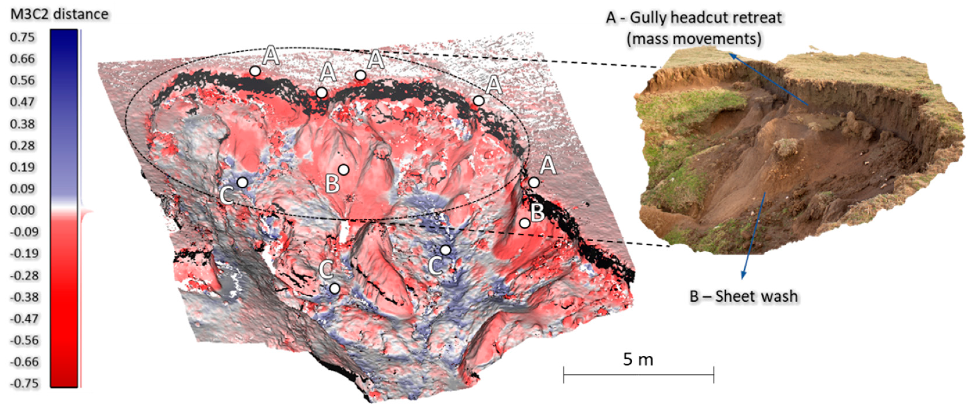
4.2. Geomorphic Implications of the Detected Erosion Induced STCs

The intensity and spatial distribution of detected STCs correspond to the results from earlier research carried out within the gully Santiš using repeat UAV photogrammetry [43]. Most detected erosion induced STCs occurred within the gully headcut, where such pronounced erosion is mostly related to mass wasting events. Detected collapse of soil material along the edge of the gully headcut (Figure 13A) is the main driver of the gradual uphill retreat of the headcut edge, which is typical of most active gullies [27,68,69,70]. Detected mass wasting is caused by gradual erosion of the headcut base, in a combination with slow sliding of the whole soil slope. Sliding of the soil sediments is caused by occasional underground runoff that forms after more intensive rainfall events at the contact of soil sediments and underlying carbonate rocks. Existence of underground flow was confirmed by the emergence of a spring at the bottom of the gully after heavy rains [43]. Recently formed parallel tension cracks are visible all along the whole current headcut edge, which indicates further propagation of the gradual uphill retreat. The intensity of gradual uphill retreat of the gully headcut corresponds to the intensity detected within earlier research [43].
The predominant low intensity of detected erosion outside of areas affected by mass wasting indicates that these areas are affected by sheet erosion, which is slowly eroding the surface of soil at the steep slopes of the gully headcut (Figure 13B). However, the intensity of such detected sheet erosion within SA-2 is very low, ranging in most cases from a few millimetres up to a centimetre or two. The presence of sheet erosion is probably related to soil crusting and desiccation cracking under the alternation of periods of long summer drought and intense rainfall events [71,72,73]. At Pag Island prolonged summer droughts are often followed by a rapid increase in precipitation amount in September and October [43], which can lead to sheet erosion and removal of surficial layers of soil affected by drought induced cracking.
Besides erosion, accumulation of material was also detected within SA-2. Absence of traces of stronger surface flow, which could transport eroded material further, indicates that most eroded material is accumulated at the first few meters from the base of the headcut (Figure 13C). The distance at which eroded material will accumulate directly depends on the ability of intermitted surface runoff to transport material away from the gully headcut [74,75], where if runoff is insufficient the material accumulates very close to the headcut. Since formation of intensive surface flow at the gully Santiš is very rare, eroded material is gradually being accumulated under the headcut, forming a talus slope (Figure 13C). If continued, such accumulation of talus slope has potential to prevent the further erosion and evolution of the gully headcut [75].

5. Conclusions

In this study, a new systematic framework for optimization of multi-temporal TLS surveys based on visibility analysis was developed and applied. The application of multi-temporal TLS surveys over the complex morphology of the gully Santiš has confirmed the accuracy, reliability and repeatability of the developed new systematic framework. Despite the very complex morphology of the gully Santiš, obstructed areas within multi-temporal TLS surveys have been minimalized, thus lowering the possibility for occurrence of shadowing effects in collected point clouds. Several important conclusions can be highlighted on the basis of carried out study:
(1)
The developed systematic framework significantly facilitated the implementation of multi-temporal TLS surveys over complex gully morphology. Although initially the systematic framework requires detailed planning and field preparation, later implementation of actual field TLS surveys is considerably facilitated.
(2)
Deviation of achieved coverage of multi-temporal TLS surveys from planned coverage was minimal within both the whole gully and the chosen part of the complex gully headcut, thus confirming the accuracy of the created survey plan and achieved repeatability of multi-temporal surveys.
(3)
A small increase in achieved deviation between planned coverage and achieved coverage was noticed between the two carried out surveys, which could be related to the rapid erosion induced STCs.
(4)
Most intense erosion induced STCs were detected within a one-year observed period within the gully headcut, where mass wasting resulted in the gradual uphill retreat of the headcut.
(5)
The developed systematic framework is applicable to all studies that require multi-temporal TLS surveys for monitoring of STCs over complex geomorphic features.
Within the future research, multi-temporal TLS surveys at gully Santiš will be continued periodically every few years. This will allow further validation of the developed framework, in which future TLS surveys will show if deviation of achieved and planned TLS coverages increases over the years.

Supplementary Materials

The following supporting information can be downloaded at: https://0-www-mdpi-com.brum.beds.ac.uk/article/10.3390/rs14143366/s1, Figure S1: Graphical scheme of TLS positioning tool (TPT) created in ModelBuilder extension of ArcGIS 10.1 software. Table S1: Precise coordinates of every permanent reference target (sphere) collected with 50-epoch RTK-GNSS measurement (Projection (EPSG): HTRS96/Croatia TM (3765)); Table S2: Difference between planned (A) and achieved (B) coverage overlap from eight chosen TLS locations for whole gully Santiš (SA-1).

Author Contributions

Conceptualization, F.D., A.Š., I.M. and L.P.; data curation, F.D.; formal analysis, F.D., A.Š., I.M. and L.P.; funding acquisition, A.Š.; investigation, F.D.; methodology, F.D., A.Š. and I.M.; project administration, A.Š.; resources, F.D.; software, F.D.; supervision, A.Š.; validation, F.D. and I.M.; visualization, F.D.; writing—original draft, F.D.; writing—review and editing, F.D., A.Š., I.M. and L.P. All authors have read and agreed to the published version of the manuscript.

Funding

This research was performed within the project UIP-2017-05-2694 financially supported by the Croatian Science Foundation.

Data Availability Statement

The data presented in this study are available on request from the corresponding author.

Acknowledgments

Authors would like to thank the Croatian Science Foundation for providing necessary research funds. Special thanks to Zoran Ivić Lola for the construction of the metal poles for mounting of permanent survey targets (spheres). Furthermore, special thanks to Marko Fabulić for the help provided with the non-systematic TLS survey carried out with Stonex x300.

Conflicts of Interest

The authors declare no conflict of interest. Preliminary results of this research were presented on the Geomorphometry 2021 international scientific conference. An extended abstract was published in the Proceedings of the Geomorphometry 2020 Conference: https://www.irpi.cnr.it/conference-files/geomorphometry-2020/59.pdf (accessed on 23 March 2022).

References

  1. Neugirg, F.; Stark, M.; Kaiser, A.; Vlacilova, M.; Della Seta, M.; Vergari, F.; Schmidt, J.; Becht, M.; Haas, F. Erosion processes in calanchi in the Upper Orcia Valley, Southern Tuscany, Italy based on multitemporal high-resolution terrestrial LiDAR and UAV surveys. Geomorphology 2016, 269, 8–22. [Google Scholar] [CrossRef]
  2. Telling, J.; Lyda, A.; Hartzell, P.; Glennie, C. Review of Earth science research using terrestrial laser scanning. Earth-Sci. Rev. 2017, 169, 35–68. [Google Scholar] [CrossRef] [Green Version]
  3. Zahs, V.; Hämmerle, M.; Anders, K.; Hecht, S.; Sailer, R.; Rutzinger, M.; Williams, J.G.; Höfle, B. Multi-temporal 3D point cloud-based quantification and analysis of geomorphological activity at an alpine rock glacier using airborne and terrestrial LiDAR. Permafr. Periglac. Processes 2019, 30, 222–238. [Google Scholar] [CrossRef]
  4. De Oliveira, C.M.M.; Francelino, M.R.; de Mendonça, B.A.F.; Ramos, I.Q. Obtaining morphometric variables from gullies using two methods of interpolation laser scanner data: The case study of Vassouras, Brazil. J. Mt. Sci. 2020, 17, 3012–3023. [Google Scholar] [CrossRef]
  5. Błaszczyk, M.; Laska, M.; Sivertsen, A.; Jawak, S.D. Combined use of aerial photogrammetry and terrestrial laser scanning for detecting geomorphological changes in Hornsund, Svalbard. Remote Sens. 2022, 14, 601. [Google Scholar] [CrossRef]
  6. Su, Y.T.; Bethel, J.; Hu, S. Octree-based segmentation for terrestrial LiDAR point cloud data in industrial applications. ISPRS J. Photogramm. Remote Sens. 2016, 113, 59–74. [Google Scholar] [CrossRef]
  7. Li, P.; Hao, M.; Hu, J.; Gao, C.; Zhao, G.; Chan, F.; Gao, J.; Dang, T.; Mu, X. Spatiotemporal Patterns of Hillslope Erosion Investigated Based on Field Scouring Experiments and Terrestrial Laser Scanning. Remote Sens. 2021, 13, 1674. [Google Scholar] [CrossRef]
  8. Gao, C.; Li, P.; Hu, J.; Yan, L.; Latifi, H.; Yao, W.; Hao, M.; Gao, J.; Dang, T.; Zhang, S. Development of gully erosion processes: A 3D investigation based on field scouring experiments and laser scanning. Remote Sens. Environ. 2021, 265, 112683. [Google Scholar] [CrossRef]
  9. Kromer, R.A.; Abellán, A.; Hutchinson, D.J.; Lato, M.; Chanut, M.A.; Dubois, L.; Jaboyedoff, M. Automated terrestrial laser scanning with near-real-time change detection–monitoring of the Séchilienne landslide. Earth Surf. Dyn. 2017, 5, 293–310. [Google Scholar] [CrossRef] [Green Version]
  10. Jiang, N.; Li, H.; Hu, Y.; Zhang, J.; Dai, W.; Li, C.; Zhou, J.W. A Monitoring Method Integrating Terrestrial Laser Scanning and Unmanned Aerial Vehicles for Different Landslide Deformation Patterns. IEEE J. Sel. Top. Appl. Earth Obs. Remote Sens. 2021, 14, 10242–10255. [Google Scholar] [CrossRef]
  11. Van Veen, M.; Hutchinson, D.J.; Kromer, R.; Lato, M.; Edwards, T. Effects of sampling interval on the frequency-magnitude relationship of rockfalls detected from terrestrial laser scanning using semi-automated methods. Landslides 2017, 14, 1579–1592. [Google Scholar] [CrossRef]
  12. DiFrancesco, P.M.; Bonneau, D.; Hutchinson, D.J. The implications of M3C2 projection diameter on 3D semi-automated rockfall extraction from sequential terrestrial laser scanning point clouds. Remote Sens. 2020, 12, 1885. [Google Scholar] [CrossRef]
  13. Fischer, M.; Huss, M.; Kummert, M.; Hoelzle, M. Application and validation of long-range terrestrial laser scanning to monitor the mass balance of very small glaciers in the Swiss Alps. Cryosphere 2016, 10, 1279–1295. [Google Scholar] [CrossRef] [Green Version]
  14. Fugazza, D.; Scaioni, M.; Corti, M.; D’Agata, C.; Azzoni, R.S.; Cernuschi, M.; Smiraglia, C.; Diolaiuti, G.A. Combination of UAV and terrestrial photogrammetry to assess rapid glacier evolution and map glacier hazards. Nat. Hazards Earth Syst. Sci. 2018, 18, 1055–1071. [Google Scholar] [CrossRef] [Green Version]
  15. Kociuba, W.; Gajek, G.; Franczak, Ł. A Short-Time Repeat TLS Survey to Estimate Rates of Glacier Retreat and Patterns of Forefield Development (Case Study: Scottbreen, SW Svalbard). Resources 2020, 10, 2. [Google Scholar] [CrossRef]
  16. Westoby, M.J.; Lim, M.; Hogg, M.; Pound, M.J.; Dunlop, L.; Woodward, J. Cost-effective erosion monitoring of coastal cliffs. Coast. Eng. 2018, 138, 152–164. [Google Scholar] [CrossRef]
  17. Hilgendorf, Z.; Marvin, M.C.; Turner, C.M.; Walker, I.J. Assessing geomorphic change in restored coastal dune ecosystems using a multi-platform aerial approach. Remote Sens. 2021, 13, 354. [Google Scholar] [CrossRef]
  18. Mavroulis, S.; Vassilakis, E.; Diakakis, M.; Konsolaki, A.; Kaviris, G.; Kotsi, E.; Kapetanidis, V.; Sakkas, V.; Alexopoulos, J.D.; Lekkas, E.; et al. The Use of Innovative Techniques for Management of High-Risk Coastal Areas, Mitigation of Earthquake-Triggered Landslide Risk and Responsible Coastal Development. Appl. Sci. 2022, 12, 2193. [Google Scholar] [CrossRef]
  19. Jones, L.K.; Kyle, P.R.; Oppenheimer, C.; Frechette, J.D.; Okal, M.H. Terrestrial laser scanning observations of geomorphic changes and varying lava lake levels at Erebus volcano, Antarctica. J. Volcanol. Geotherm. Res. 2015, 295, 43–54. [Google Scholar] [CrossRef] [Green Version]
  20. De Zeeuw-van Dalfsen, E.; Richter, N.; González, G.; Walter, T.R. Geomorphology and structural development of the nested summit crater of Láscar Volcano studied with Terrestrial Laser Scanner data and analogue modelling. J. Volcanol. Geotherm. Res. 2017, 329, 1–12. [Google Scholar] [CrossRef]
  21. Santagata, T. Monitoring of the Nirano Mud Volcanoes Regional Natural Reserve (North Italy) using unmanned aerial vehicles and terrestrial laser scanning. J. Imaging 2017, 3, 42. [Google Scholar] [CrossRef] [Green Version]
  22. Eltner, A.; Mulsow, C.; Maas, H.G. Quantitative measurement of soil erosion from TLS and UAV data. Int. Arch. Photogramm. Remote Sens. Spat. Inf. Sci. 2013, 40, 4–6. [Google Scholar] [CrossRef] [Green Version]
  23. Vinci, A.; Brigante, R.; Todisco, F.; Mannocchi, F.; Radicioni, F. Measuring rill erosion by laser scanning. Catena 2015, 124, 97–108. [Google Scholar] [CrossRef]
  24. Sun, L.; Wu, S.; Zhang, B.; Lei, Q. Development of rill erosion and its simulation with cellular automata-rill model in Chinese Loess Plateau. Arch. Agron. Soil Sci. 2021, 68, 823–837. [Google Scholar] [CrossRef]
  25. Li, Y.; Lu, X.; Washington-Allen, R.A.; Li, Y. Microtopographic Controls on Erosion and Deposition of a Rilled Hillslope in Eastern Tennessee, USA. Remote Sens. 2022, 14, 1315. [Google Scholar] [CrossRef]
  26. Perroy, R.L.; Bookhagen, B.; Asner, G.P.; Chadwick, O.A. Comparison of gully erosion estimates using airborne and ground-based LiDAR on Santa Cruz Island, California. Geomorphology 2010, 118, 288–300. [Google Scholar] [CrossRef]
  27. Rengers, F.K.; Tucker, G.E. The evolution of gully headcut morphology: A case study using terrestrial laser scanning and hydrological monitoring. Earth Surf. Processes Landf. 2015, 40, 1304–1317. [Google Scholar] [CrossRef]
  28. Goodwin, N.R.; Armston, J.; Stiller, I.; Muir, J. Assessing the repeatability of terrestrial laser scanning for monitoring gully topography: A case study from Aratula, Queensland, Australia. Geomorphology 2016, 262, 24–36. [Google Scholar] [CrossRef]
  29. Goodwin, N.R.; Armston, J.D.; Muir, J.; Stiller, I. Monitoring gully change: A comparison of airborne and terrestrial laser scanning using a case study from Aratula, Queensland. Geomorphology 2017, 282, 195–208. [Google Scholar] [CrossRef]
  30. Castillo, C.; Pérez, R.; James, M.R.; Quinton, J.N.; Taguas, E.V.; Gómez, J.A. Comparing the accuracy of several field methods for measuring gully erosion. Soil Sci. Soc. Am. J. 2012, 76, 1319–1332. [Google Scholar] [CrossRef] [Green Version]
  31. Taylor, R.J.; Massey, C.; Fuller, I.C.; Marden, M.; Archibald, G.; Ries, W. Quantifying sediment connectivity in an actively eroding gully complex, Waipaoa catchment, New Zealand. Geomorphology 2018, 307, 24–37. [Google Scholar] [CrossRef]
  32. Vericat, D.; Smith, M.W.; Brasington, J. Patterns of topographic change in sub-humid badlands determined by high resolution multi-temporal topographic surveys. Catena 2014, 120, 164–176. [Google Scholar] [CrossRef]
  33. Marsico, A.; De Santis, V.; Capolongo, D. Erosion Rate of the Aliano Biancana Badlands Based on a 3D Multi-Temporal High-Resolution Survey and Implications for Wind-Driven Rain. Land 2021, 10, 828. [Google Scholar] [CrossRef]
  34. Camera, C.; Djuma, H.; Bruggeman, A.; Zoumides, C.; Eliades, M.; Charalambous, K.; Abate, D.; Faka, M. Quantifying the effectiveness of mountain terraces on soil erosion protection with sediment traps and dry-stone wall laser scans. Catena 2018, 171, 251–264. [Google Scholar] [CrossRef]
  35. Meinen, B.U.; Robinson, D.T. Where did the soil go? Quantifying one year of soil erosion on a steep tile-drained agricultural field. Sci. Total Environ. 2020, 729, 138320. [Google Scholar] [CrossRef]
  36. Neugirg, F.; Kaiser, A.; Huber, A.; Heckmann, T.; Schindewolf, M.; Schmidt, J.; Becht, M.; Haas, F. Using terrestrial LiDAR data to analyse morphodynamics on steep unvegetated slopes driven by different geomorphic processes. Catena 2016, 142, 269–280. [Google Scholar] [CrossRef]
  37. Kasperski, J.; Delacourt, C.; Allemand, P.; Potherat, P.; Jaud, M.; Varrel, E. Application of a terrestrial laser scanner (TLS) to the study of the Séchilienne Landslide (Isère, France). Remote Sens. 2010, 2, 2785–2802. [Google Scholar] [CrossRef] [Green Version]
  38. Bremer, M.; Sass, O. Combining airborne and terrestrial laser scanning for quantifying erosion and deposition by a debris flow event. Geomorphology 2012, 138, 49–60. [Google Scholar] [CrossRef]
  39. Alexiou, S.; Deligiannakis, G.; Pallikarakis, A.; Papanikolaou, I.; Psomiadis, E.; Reicherter, K. Comparing high accuracy t-LiDAR and UAV-SfM derived point clouds for geomorphological change detection. ISPRS Int. J. Geo-Inf. 2021, 10, 367. [Google Scholar] [CrossRef]
  40. Li, Y.; McNelis, J.J.; Washington-Allen, R.A. Quantifying Short-Term Erosion and Deposition in an Active Gully Using Terrestrial Laser Scanning: A Case Study from West Tennessee, USA. Front. Earth Sci. 2020, 8, 481. [Google Scholar] [CrossRef]
  41. Gómez-Gutiérrez, Á.; Biggs, T.; Gudino-Elizondo, N.; Errea, P.; Alonso-González, E.; Nadal Romero, E.; de Sanjosé Blasco, J.J. Using visibility analysis to improve point density and processing time of SfM-MVS techniques for 3D reconstruction of landforms. Earth Surf. Processes Landf. 2020, 45, 2524–2539. [Google Scholar] [CrossRef]
  42. Lončar, N. Geomorphologic regionalization of the central and southern parts of Pag Island. Geoadria 2009, 14, 5–25. [Google Scholar] [CrossRef]
  43. Šiljeg, A.; Domazetović, F.; Marić, I.; Lončar, N.; Panđa, L. New method for automated quantification of vertical spatio-temporal changes within gully cross-sections based on very-high-resolution models. Remote Sens. 2021, 13, 321. [Google Scholar] [CrossRef]
  44. Domazetović, F.; Šiljeg, A.; Lončar, N.; Marić, I. Development of automated multicriteria GIS analysis of gully erosion susceptibility. Appl. Geogr. 2019, 112, 102083. [Google Scholar] [CrossRef]
  45. Carr, S.; Douglas, B.; Phillips, D. Terrestrial Laser Scanning (TLS) Field Camp Manual; UNAVCO: Boulder, CO, USA, 2013. [Google Scholar]
  46. Faro. Technical Specification Sheet for the Focus Laser Scanner. 2022. Available online: https://knowledge.faro.com/Hardware/3D_Scanners/Focus/Technical_Specification_Sheet_for_the_Focus_Laser_Scanner (accessed on 25 April 2022).
  47. ESRI. Using Viewshed and Observer Points for Visibility Analysis. 2022. Available online: https://pro.arcgis.com/en/pro-app/2.8/tool-reference/3d-analyst/using-viewshed-and-observer-points-for-visibility.htm (accessed on 30 April 2022).
  48. Wu, H.; Pan, M.; Yao, L.; Luo, B. A partition-based serial algorithm for generating viewshed on massive DEMs. Int. J. Geogr. Inf. Sci. 2007, 21, 955–964. [Google Scholar] [CrossRef]
  49. Lee, S.B.; Ryu, J.R.; Choo, S.Y.; Woo, S.H.; Seo, J.H.; Jo, J.S. A Study on Viewshed Frequency Analysis for Establishing Viewpoints. In Proceedings of the FUTURE CITIES 28th eCAADe Conference Proceedings, Zurich, Switzerland, 15–18 September 2010. [Google Scholar]
  50. Cook, K.L. An evaluation of the effectiveness of low-cost UAVs and structure from motion for geomorphic change detection. Geomorphology 2017, 278, 195–208. [Google Scholar] [CrossRef]
  51. James, M.R.; Robson, S.; Smith, M.W. 3-D uncertainty-based topographic change detection with structure-from-motion photogrammetry: Precision maps for ground control and directly georeferenced surveys. Earth Surf. Processes Landf. 2017, 42, 1769–1788. [Google Scholar] [CrossRef]
  52. Cândido, B.M.; James, M.; Quinton, J.; Lima, W.D.; Silva, M.L.N. Sediment source and volume of soil erosion in a gully system using UAV photogrammetry. Rev. Bras. De Ciência Do Solo 2020, 44, 1–14. [Google Scholar] [CrossRef]
  53. Bailey, G.; Li, Y.; McKinney, N.; Yoder, D.; Wright, W.; Washington-Allen, R. Las2DoD: Change Detection Based on Digital Elevation Models Derived from Dense Point Clouds with Spatially Varied Uncertainty. Remote Sens. 2022, 14, 1537. [Google Scholar] [CrossRef]
  54. Williams, J.G.; Anders, K.; Winiwarter, L.; Zahs, V.; Höfle, B. Multi-directional change detection between point clouds. ISPRS J. Photogramm. Remote Sens. 2021, 172, 95–113. [Google Scholar] [CrossRef]
  55. Winiwarter, L.; Anders, K.; Höfle, B. M3C2-EP: Pushing the limits of 3D topographic point cloud change detection by error propagation. ISPRS J. Photogramm. Remote Sens. 2021, 178, 240–258. [Google Scholar] [CrossRef]
  56. Zahs, V.; Winiwarter, L.; Anders, K.; Williams, J.G.; Rutzinger, M.; Höfle, B. Correspondence-driven plane-based M3C2 for lower uncertainty in 3D topographic change quantification. ISPRS J. Photogramm. Remote Sens. 2022, 183, 541–559. [Google Scholar] [CrossRef]
  57. Lague, D.; Brodu, N.; Leroux, J. Accurate 3D comparison of complex topography with terrestrial laser scanner: Application to the Rangitikei canyon (NZ). ISPRS J. Photogramm. Remote Sens. 2013, 82, 10–26. [Google Scholar] [CrossRef] [Green Version]
  58. Barnhart, T.B.; Crosby, B.T. Comparing two methods of surface change detection on an evolving thermokarst using high-temporal-frequency terrestrial laser scanning, Selawik River, Alaska. Remote Sens. 2013, 5, 2813–2837. [Google Scholar] [CrossRef] [Green Version]
  59. Gomez-Gutierrez, A.; Schnabel, S.; Berenguer-Sempere, F.; Lavado-Contador, F.; Rubio-Delgado, J. Using 3D photo-reconstruction methods to estimate gully headcut erosion. Catena 2014, 120, 91–101. [Google Scholar] [CrossRef]
  60. Gómez-Gutiérrez, Á.; Gonçalves, G.R. Surveying coastal cliffs using two UAV platforms (multirotor and fixed-wing) and three different approaches for the estimation of volumetric changes. Int. J. Remote Sens. 2020, 41, 8143–8175. [Google Scholar] [CrossRef]
  61. Kromer, R.A.; Abellán, A.; Hutchinson, D.J.; Lato, M.; Edwards, T.; Jaboyedoff, M. A 4D filtering and calibration technique for small-scale point cloud change detection with a terrestrial laser scanner. Remote Sens. 2015, 7, 13029–13052. [Google Scholar] [CrossRef] [Green Version]
  62. Duffy, J.P.; Shutler, J.D.; Witt, M.J.; DeBell, L.; Anderson, K. Tracking fine-scale structural changes in coastal dune morphology using kite aerial photography and uncertainty-assessed structure-from-motion photogrammetry. Remote Sens. 2018, 10, 1494. [Google Scholar] [CrossRef] [Green Version]
  63. Esposito, G.; Mastrorocco, G.; Salvini, R.; Oliveti, M.; Starita, P. Application of UAV photogrammetry for the multi-temporal estimation of surface extent and volumetric excavation in the Sa Pigada Bianca open-pit mine, Sardinia, Italy. Environ. Earth Sci. 2017, 76, 1–16. [Google Scholar] [CrossRef]
  64. Riverscapes Consortium. Geomorphic Change Detection Software. 2020. Available online: http://gcd.riverscapes.xyz/ (accessed on 18 September 2020).
  65. Wheaton, J.M.; Brasington, J.; Darby, S.E.; Sear, D.A. Accounting for uncertainty in DEMs from repeat topographic surveys: Improved sediment budgets. Earth surface processes and landforms. J. Br. Geomorphol. Res. Group 2010, 35, 136–156. [Google Scholar] [CrossRef]
  66. Williams, R. DEMs of difference. Geomorphol. Tech. 2012, 2, 1–17. [Google Scholar]
  67. Alfonso-Torreño, A.; Schnabel, S.; Gómez-Gutiérrez, Á.; Crema, S.; Cavalli, M. Effects of gully control measures on sediment yield and connectivity in wooded rangelands. Catena 2022, 214, 106259. [Google Scholar] [CrossRef]
  68. Gutiérrez, Á.G.; Schnabel, S.; Contador, F.L. Gully erosion, land use and topographical thresholds during the last 60 years in a small rangeland catchment in SW Spain. Land Degrad. Dev. 2009, 20, 535–550. [Google Scholar] [CrossRef]
  69. Vanmaercke, M.; Poesen, J.; Van Mele, B.; Demuzere, M.; Bruynseels, A.; Golosov, V.; Bezerra, J.F.R.; Bolysov, S.; Dvinskih, A.; Frankl, A.; et al. How fast do gully headcuts retreat? Earth-Sci. Rev. 2016, 154, 336–355. [Google Scholar] [CrossRef]
  70. Castillo, C.; Gómez, J.A. A century of gully erosion research: Urgency, complexity and study approaches. Earth-Sci. Rev. 2016, 160, 300–319. [Google Scholar] [CrossRef]
  71. Ran, Q.; Su, D.; Li, P.; He, Z. Experimental study of the impact of rainfall characteristics on runoff generation and soil erosion. J. Hydrol. 2012, 424, 99–111. [Google Scholar] [CrossRef]
  72. Samani, A.N.; Ahmadi, H.; Jafari, M.; Boggs, G.; Ghoddousi, J.; Malekian, A. Geomorphic threshold conditions for gully erosion in Southwestern Iran (Boushehr-Samal watershed). J. Asian Earth Sci. 2009, 35, 180–189. [Google Scholar] [CrossRef]
  73. Bora, M.J.; Bordoloi, S.; Pekkat, S.; Garg, A.; Sekharan, S.; Rakesh, R.R. Assessment of soil erosion models for predicting soil loss in cracked vegetated compacted surface layer. Acta Geophys. 2022, 70, 333–347. [Google Scholar] [CrossRef]
  74. Kirkby, M.J.; Bracken, L.J. Gully processes and gully dynamics. Earth Surf. Processes Landf. J. Br. Geomorphol. Res. Group 2009, 34, 1841–1851. [Google Scholar] [CrossRef]
  75. Chaplot, V. Impact of terrain attributes, parent material and soil types on gully erosion. Geomorphology 2013, 186, 1–11. [Google Scholar] [CrossRef]
Figure 1. Study area covering complex morphology of gully Santiš ((A)—location of Pag Island within Croatia; (B)—location of gully Santiš within geological map of Pag Island (1—Water; 2Holocen deposits; 3Limestone breccia; 4—Flysch; 5Foraminiferal limestones; 6Rudist limestones)).
Remotesensing 14 03366 g001
Figure 2. Four main steps of a new systematic framework for optimization of multi-temporal terrestrial LiDAR surveys.
Remotesensing 14 03366 g002
Figure 3. Faro Focus M70 terrestrial laser scanner used for multi-temporal point cloud acquisition (A); Design of metal poles for mounting of permanent survey targets (spheres) to the preferred height (B) (a & b—metal poles; c—adapter for sphere; d—adapter for RTK-GPS antenna; e—standard sphere; f—sphere center; g—RTK-GPS antenna bottom).
Remotesensing 14 03366 g003
Figure 4. Coverage planned by TPT based on visibility analysis within the rough terrain of gully headcut (A); visibility check (line of sight) for permanent and auxiliary targets around TLS position 1 (B).
Remotesensing 14 03366 g004
Figure 5. Methodology applied for preparation of seven PTPs distributed around the gully Santiš ((A)—carving of PMPs in carbonate badrock with hammer drill; (B)—leveling of PMPs with self-leveling concrete (B①—anchors drilled in concrete; B② and B③—plastic cover of metal anchors for preventing corrosion; B④—leveled base of metal poles); (C)—plaster cap created for long-term protection of PTPs (C①—metal anchors; C②—whole for measurement with RTK-GPS; C③—gypsum protective cap); (D)—installation of target (sphere) on metal pole fixed to the PTP (D①—target (sphere); D②—designed metal pole; D③—PTP); (E)—example of permanent target fixed at the height of 210 cm above planned PTP).
Remotesensing 14 03366 g005
Figure 6. Methodology applied for processing of multi-temporal LiDAR data in Faro SCENE software.
Remotesensing 14 03366 g006
Figure 7. Stonex X300 TLS (A) used for the non-systematic TLS survey over gully Santiš (B) in 2017.
Remotesensing 14 03366 g007
Figure 8. Point clouds created from carried out multi-temporal TLS surveys ((A)—point cloud of whole gully (SA-1) (Parts of point cloud for SA-1 with purple texture were collected after the twilight, which caused errors in stored texture information); (B,C) point clouds of chosen part of gully headcut (SA-2) used for detection and quantification of STCs).
Remotesensing 14 03366 g008
Figure 9. Difference between planned (A) and achieved (B) scan overlap for whole gully Santiš (SA-1).
Remotesensing 14 03366 g009
Figure 10. Deviation of planned and achieved coverage for every individual TLS position ((A)—Deviation of initial TLS survey of whole gully Santiš (SA-1); (B)—Deviation of initial TLS survey of gully headcut (SA-2); (C)—Deviation of second TLS survey of gully headcut (SA-2)) and difference in achieved coverage of gully headcut (SA-2) between TLS survey 2019 and TLS survey 2020 (D).
Remotesensing 14 03366 g010
Figure 11. Comparison between the standard deviation of two multi-temporal point clouds (initial TLS survey (left) and final TLS survey (right)).
Remotesensing 14 03366 g011
Figure 12. Histogram of all STCs detected by M3C2 algorithm (A); Gaussian distribution of all STCs detected by M3C2 algorithm (B); negative STCs (erosion) detected by M3C2 algorithm (C); positive STCs (accumulation) detected by M3C2 algorithm (D).
Remotesensing 14 03366 g012
Figure 13. Point cloud representing the soil erosion induced STCs (M3C2 distance) between December 2019 and December 2020 (Amass wasting; Bsheet erosion; Cmaterial accumulation below gully headcut).
Remotesensing 14 03366 g013
Figure 14. Visual comparison between point clouds covering identical part of gully headcut ((A)—point cloud created by traditional non-systematic approach; (B)—point cloud created through developed optimization framework).
Remotesensing 14 03366 g014
Table 1. Planned coverage of the study area from eight chosen optimal TLS positions.
Survey Positions 1Gully
Coverage (m2)
Percentage (%)Gully Headcut
Coverage (m2)
Percentage (%)
TLS position 1566.9646.21167.1483.89
TLS position 2578.9447.18157.3778.99
TLS position 3410.5033.4699.9350.16
TLS position 4547.8544.6580.2340.27
TLS position 5521.0142.46--
TLS position 6382.2531.15--
TLS position 7540.9644.09--
TLS position 8381.6331.10--
Total coverage1190.0496.99193.4997.12
1 Optimal TLS positions chosen based on performed visibility analysis with developed TPT tool.
Table 2. Difference in total planned and achieved coverage for TLS survey 2019 over whole gully (SA-1).
Survey PositionsPlanned CoverageAchieved Coverage
Gully
Coverage (m2)
Percentage (%)Gully
Coverage (m2)
Percentage (%)
TLS position 1566.9646.21540.4744.05
TLS position 2578.9447.18498.8140.65
TLS position 3410.5033.46407.1833.19
TLS position 4547.8544.65471.7238.45
TLS position 5521.0142.46439.1835.79
TLS position 6382.2531.15361.9429.50
TLS position 7540.9644.09414.1133.75
TLS position 8381.6331.10311.8625.42
Total coverage1190.0496.991181.0796.26
Table 3. Difference in total planned and achieved coverage for both TLS surveys over gully headcut (SA-2).
Gully HeadcutTLS
Positions
Total Area (m2)No of PointsCovered Area
(m2)
Covered Area (%)
Planned coverageP1–P4199.23-197.4399.10
TLS survey 1P1–P4199.2325,875,206195.7098.23
TLS survey 2P1–P4199.232,665,029193.4997.12
Table 4. Point cloud statistics calculated by M3C2 for performed multi-temporal TLS surveys.
Survey Point Cloud Characteristics
Total Number of PointsAverage Point Density (No/m2)SD (RMSE)Mean TLS
Survey Error
TLS-201925,875,20692,411.45 0.4 (0.7) cm1.29 cm
TLS-20202,665,02995,179.631.5 (1.8) cm1.37 cm
Publisher’s Note: MDPI stays neutral with regard to jurisdictional claims in published maps and institutional affiliations.

