Multimodal Fusion of Mobility Demand Data and Remote Sensing Imagery for Urban Land-Use and Land-Cover Mapping

Abstract

This paper aims at exploring the potentiality of the multimodal fusion of remote sensing imagery with information coming from mobility demand data in the framework of land-use mapping in urban areas. After a discussion on the function of mobility demand data, a probabilistic fusion framework is developed to take advantage of remote sensing and transport data, and their joint use for urban land-use and land-cover applications in urban and surrounding areas. Two different methods are proposed within this framework, the first based on pixelwise probabilistic decision fusion and the second on the combination with a region-based multiscale Markov random field. The experimental validation is conducted on a case study associated with the city of Genoa, Italy.

1. Introduction

Land-use and land-cover mapping in urban and peri-urban areas plays a major role in applications to urban planning, urban sprawl mitigation, and disaster risk prevention in human settlements [1]. The discrimination of urban land-use classes is a complex task, given the difficulty of jointly defining complex spatial patterns found in remote sensing data and their relation to the semantic use of the corresponding urban area [2,3,4]. In this framework, the introduction of ancillary information, for example OpenStreetMap (OSM) layers, cadastral data, or social media data, used conjointly with remote sensing data has shown promising results [5,6,7]. The objective of this work is to explore the potential of the fusion of remote sensing data with information related to the so-called mobility demand, such as people and freight mobility needs, for applications of urban land-use and land-cover mapping in urban and peri-urban areas.The technique proposed in this paper combines methodological aspects of two different disciplinary areas which are generally considered separately, namely remote sensing and transport systems engineering. In this case, the latter is considered the set of methods and tools aimed at connecting the so-called activity system, i.e., the set of activities (work, residence, mixed) performed in the different urban zones [8].

In this framework, a probabilistic decision fusion strategy [9] is adopted in the proposed approach and two supervised methods are developed. In the first one, a case-specific probabilistic model is developed to fuse, on a pixelwise basis, posterior probability distributions computed from the mobility and remote sensing data sources with regard to the urban land-use and land-cover classes, respectively. In the second method, the multiscale region-based Markov random field (MRF) model in [10] is extended to integrate the aforementioned pixelwise probabilistic model and the spatial structure associated with the transport data. This second method allows for characterising spatial-contextual information within the process of urban land-use and land-cover mapping, an especially important task in the application to high-resolution remote sensing images [11].

The novel contributions of this paper are twofold. First, the potential of the integration, in a multimodal fusion framework, of methodological contributions coming from the remote-sensing and transport-systems engineering fields is investigated and experimentally discussed. The analysis of the advantages of this fusion process and of the added value of mobility data are performed in the framework of the challenging problem of urban land-use mapping from Earth observation (EO) imagery. Second, two novel algorithms are developed to address the combination of remote sensing and transport data for urban land-use mapping by leveraging probabilistic modelling and Markovian multiscale concepts. To the authors’ knowledge, this is the first study in which the joint use of remote-sensing images and mobility demand data, the latter usually gathered in the so-called Origin-Destination (OD) matrix [8], is proposed and validated in a case study of urban land-use and land-cover mapping. A preliminary version of the present work was published by two of the authors of this article in the conference paper [12]. The present article further extends this previous paper by expanding both the methodological discussion and the experimental validation of the proposed approach in the aforementioned case study.

The objective of the present work is to demonstrate the effectiveness of the novel combination of satellite imagery and mobility demand data for urban land-use and land-cover mapping in the context of urban applications, as well as to propose two novel algorithms that address this fusion problem. This work also has relevance to transport-system studies, as it demonstrates an additional value of the OD matrix, showing that it can provide information not only related to the mobility demand (which represents its currently primary use in transport analysis and planning) but also to the activities performed in the different zones of an urban area, and thus to the urban land use.

In this framework, the proposed approach, introducing the fusion of transport-data and remote-sensing images, is not meant as an alternative to the use of cadastral data, but as a further source of information, complementary to what can be extracted by cadastre. Cadastral data sets obviously play a crucial role in urban mapping applications. As a matter of fact, thematic products generated by the proposed methods could be used by the local authorities as an additional tool for evaluating the goodness of cadastral data and to extract up-to-date land-use maps when cadastral data are unavailable or not fully reliable. Moreover, the availability of up-to-date OD matrices allows to plot the variations and the dynamic evolution of the urban land use over time in a way that is more difficult if only cadastral data can be used.

In this connection, the recent literature in transportation studies also shows how OD matrices can be estimated and kept up-to-date in quasi-real time, thus further supporting the role of the proposed approaches as complementary thematic mapping tools, in addition to cadastral data sets. Such a direct dynamic estimation of OD matrices can be accomplished using a wide range of crowdsourced data that are becoming more and more widespread, including traffic counts data, smartcard data [13], GPS data [14], mobile phone data [15], and floating car data provided by probe vehicles [16]. From this perspective, the possibility of estimating OD matrices from the aforementioned sources without prior knowledge on the territory suggests the relevance of exploring the possible benefit coming from their joint use with remote-sensing imagery. In addition, mobility data are also available—or can be estimated as mentioned above—in the urban areas where cadastral data may be unavailable, unreliable, or not up-to-date. Indeed, cadastral data can be affected by unreliability issues deriving from variations on the ground, owners negligence in updating household data, or insufficiently frequent updates by the municipalities; there might also be a lack of detailed regulations to verify these kinds of data [17].

The paper is organised as follows: The previous work related to the addressed topics is reviewed in Section 2. Then, Section 3 recalls basic concepts about transport systems and mobility demand data. The considered case study, with its associated datasets, and the methodological formulation of the proposed techniques are described in Section 4. The experimental results obtained by the developed methods and by baseline approaches are reported in Section 5 and discussed in Section 6. Finally, conclusions are drawn in Section 7.

2. Previous Work

The issues addressed in this paper consist of the fusion of the information derived from two separate scientific areas, transport systems engineering and remote sensing, to investigate the potential of the joint use of two different types of data for the specific application of mapping land use and land cover in urban and peri-urban areas. In this section, we shall review the state of the art associated with remote sensing and ancillary data fusion—jointly—focusing on approaches developed for urban land-use purposes. Land use is of great importance for urban planning, environmental monitoring, and transportation management [18].

Remote sensing techniques for land-cover and land-use mapping applications have been regarded as a major solution for urban planning and monitoring of the urban environment [19,20,21]. An important role in this context is played by supervised classification methods. Spatially dense image classification (or semantic segmentation) methods based on architectures of deep neural networks have recently found to be highly promising in a variety of applications, including remote sensing [22,23]. However, to perform accurate classification, deep-learning based classifiers usually require a large number of training samples, which may not be available for many remote sensing applications [24] and especially with regard to land-use classes [5].

At the same time, crowd-sourced OSM data provide rich annotation information about urban targets [19,25]. The combination of OSM data and remote-sensing images for efficient urban scene classification has been explored recently [19,26,27]. For example, in [26], Landsat images were integrated with OSM data in a semiautomatic large-scale and long-time series urban land mapping framework with the goal of sustainable urban development. Road networks play an important role in traffic management, urban planning, vehicle navigation, and emergency management. In [27], an automatic approach for extracting road networks from very high resolution (VHR) remote sensing images and OSM data was presented based on a fully convolutional neural network, in which the road centrelines from OSM were employed to construct the labels for the model training and validation.

Furthermore, the quantification of impervious surfaces provides useful information for urban planning and therefore socioeconomic development [28,29,30,31,32,33]. OSM data on impervious surfaces have been integrated with the predictions of neural networks, when applied to Landsat 8 images, to produce classification results on impervious surfaces [28] and to Sentinel-2 multispectral imagery [29]. In [30], a further road superimposition strategy that considers road hierarchy was developed to perform land-cover classification of urban areas. Moreover, a hybrid method was developed to improve the extraction of impervious surfaces from high-resolution aerial imagery in [31], integrating ancillary datasets from OSM, and the United States National Wetland Inventory and National Cropland Data to generate training and validation samples in a semiautomatic manner.

These methods, however, simply consider information about impervious surfaces, without including knowledge about their use. OSM road network data were also integrated with remote sensing and geospatial data to develop an accurate urban functional region identification method and to analyse the spatial distribution of the population, information crucial to the analysis of population mobility patterns and health indicators [34]. The distribution of the population is of great significance in urban emergency response, disaster assessment, urban planning, and transportation route design [35]. In [35], land cover and ancillary data, including building addresses, housing price data, and stereo pairs of high-resolution remote sensing images, were used to simulate fine-scale urban population distribution.

Street blocks generated from OSM data have been used in [36] as the minimum classification unit and integrated with ensemble learning and with sets of multiscale spatially explicit data about land surface, vertical height, socioeconomic attributes, social media, demography, and topography, to derive urban land-use classification maps to be used for urban planning, environmental management, and disaster control [36]. Furthermore, this information regarding land use in the urban environment has been integrated with data about population, roads, and other transportation infrastructure to analyse land transitions in periods of fast economic growth [37].

Studies on land-cover change and urban growth have also been conducted by fusing remote sensing information with ancillary OSM data [38]. Modelling land-use changes is one way to manage the consequences of the expansion of urban areas. In [39], land-use data were integrated with a cellar automation model (slope, land use, exclusion/attraction, urban extent, transportation, and hillshade–SLEUTH) to reveal trends in urban growth for the different development scenarios [39]. For example, a key factor towards sustainable urban development is the understanding of the interdependencies among urban growth patterns, infrastructure, and socioeconomic indicators [40]. In [40], the spatiotemporal urban growth dynamics and their relation to road density were studied through urban land-cover maps and OSM data to generate road density maps and the SLEUTH urban growth model.

The availability of remote sensing data has opened up opportunities for modelling techniques that allow to understand how subtle differences in the urban fabric can impact transportation mode shares [41]. A combination of remote sensing imagery and mobile phone positioning data (MPPD) through a support vector machine was considered in [18] to generate land-use maps. Based on the resulting land-use maps and on the MPPD, the activity density in key zones during daytime and nighttime was analysed to illustrate the volume and variation of people working and living across different regions.

The aforementioned state-of-the-art techniques mostly focus on the computation of land-cover and land-use maps from input remote sensing and ancillary datasets in which transport engineering is only weakly involved, namely, through the simple topology of road networks or the flux of population, which do not convey any direct information regarding land use. From this perspective, a major novelty of the proposed method consists precisely of the combination of remote sensing with traffic data—hence offering details about mobility demand and the related use of the associated portions of the urban land.

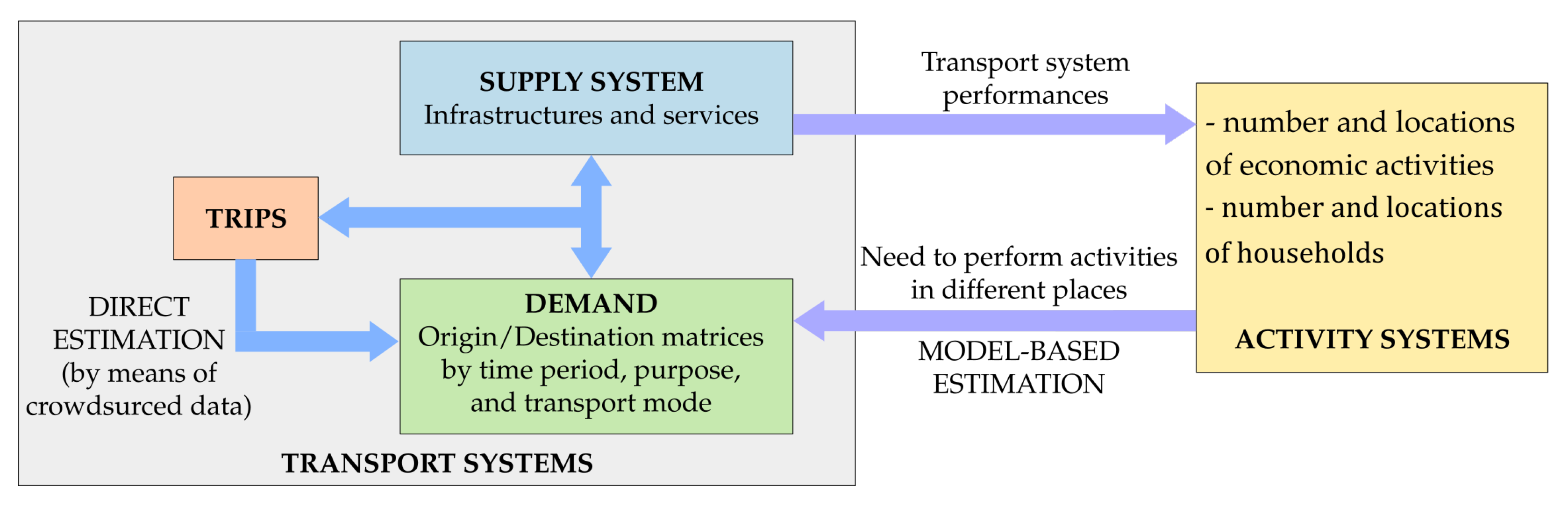
3. Basics on Transport Systems and Mobility Demand Data

The aim of this section is to recall and discuss the mobility demand and its relevance in the proposed methodology for urban land-use classification. Mobility demand consists of the collection of people and freight, namely users that need to move from one location to another for a specific purpose, such as “go to work”, “go to school”, “return home”, “spend free time”, etc. These travel needs are satisfied by the supply system, which consists of the set of infrastructures (e.g., roads, rails, etc.) and services (e.g., public transport, etc.) providing trip solutions to the users. In this connection, it is common to refer to these solutions in terms of “transport mode alternatives” (hereafter indicated also as “transport alternatives”) determined by different combinations of infrastructures and services such as private car, motorbike, pedestrian, rail transport, etc.

The mobility demand and the supply system, which represent the two components of a transport system, are highly connected and interact with each other (e.g., an efficient public transport system can attract users from other transport modes, such as private vehicles) and with the so-called activity system, which consists of residences, economic activities (e.g., work, education, shopping, etc.), as well as the relevant locations (e.g., offices and/or factories, schools, and shops).

A basic scheme of a generic transport system is depicted in Figure 1, where it is possible to note the feedback mechanism showing that the distribution of the activities in an area determines the need for trips (i.e., the demand) and the supply performances determine the ease of reaching/leaving the locations of the activities themselves. For example, travel needs depend on the level and location of economic activities households. Conversely, in a medium/long time period, the location of economic activities and households is influenced by the transport supply, whose performances determine their accessibility (e.g., a shopping centre tends to be located in a place that can be rapidly and cheaply reached by customers, such as in the proximity of fast roads or subway stations).

Since the mobility demand originates from the need to perform different activities in different places, it is always spatially referred to a pair of locations, namely an origin and a destination. In addition, since different activities are performed at different times of the day, it is also useful to consider a reference time period (e.g., an hour of the day). Accordingly, considering the purpose associated with the trip need (such as “going to work”, “going home after work”, etc.) can provide information about the activities that are performed in different locations. From the above considerations, it descends that it is possible to identify the collection of user trips between a certain origin/destination pair travelling for a given purpose in a given time period.

Mobility data are usually available for cities and regions, and are traditionally obtained via census samples, ad-hoc surveys, and calibrated models representing users’ travel choices in terms of destination, transport mode, and purpose (see Figure 1). For more details about mobility demand, its relationships with the supply and the activity system and the abovementioned techniques for demand estimation, readers can refer to [8]. Here, we recall that, as mentioned above, the increasing availability of crowdsourced data provides the capability for updating the mobility data in quasi-real time, thus not only capturing the demand variations over time but also obtaining reliable mobility demand data estimates without the need for models. In particular, such sources focus directly on the trips within the urban area, which are generated by the combination of demand and supply (see Figure 1), being such a combination known as “assignment” in the transport systems literature [8]. As a consequence, trips implicitly include information on the demand as well.

In the following subsections, more details about the characteristics of mobility demand are discussed in connection to the information they can provide to the identification of urban land use.

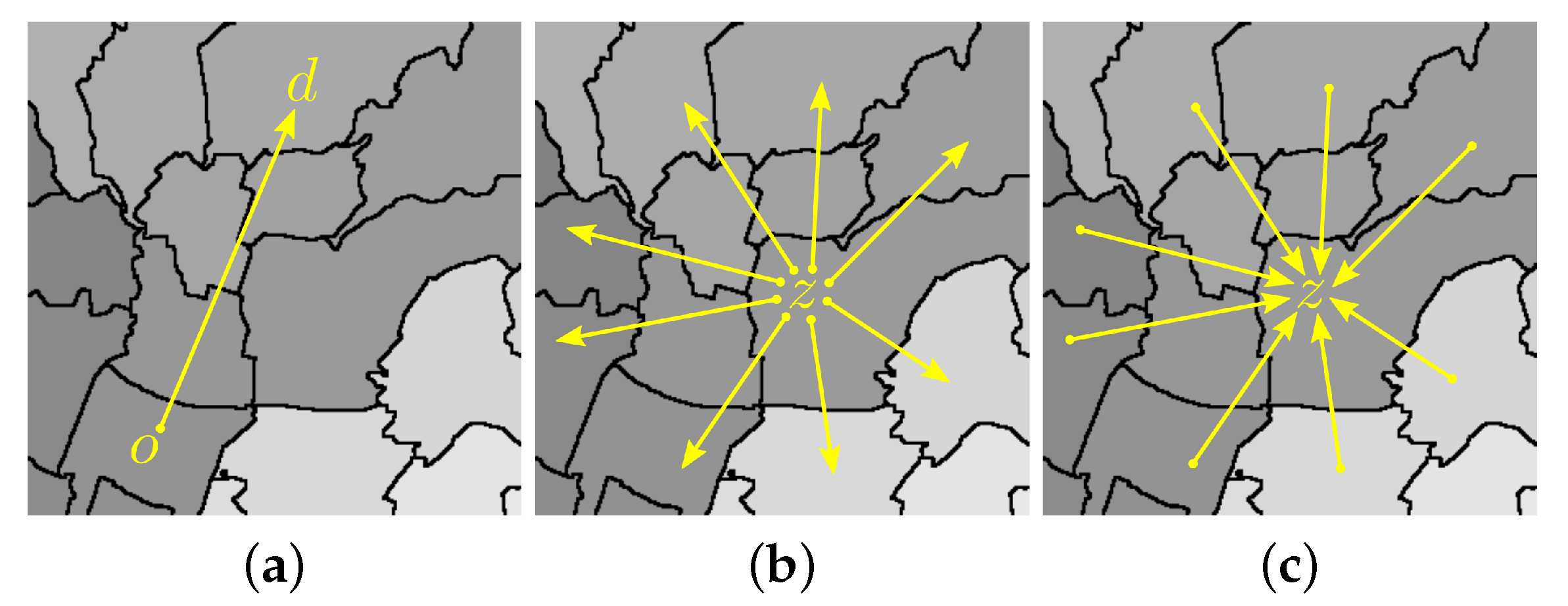
3.1. Mobility Demand Spatial Characteristics

Since travel needs in a certain area may, in general, start and end in a large number of different locations, the considered study area is always spatially discretised into N zones, and only travel needs between different zones are collected. An example of zoning is reported in Figure 2, where it is possible to note that the zones can be significantly different in size, usually as a consequence of the population and economic activity densities.

The zones are determined considering different criteria, such as the presence of physical barriers (e.g., rivers, railways, roads, …) and the available census data. A general criterion is that the zones are the most homogeneous as possible with respect to the activities performed therein, such as residential, working, and commercial. On the one hand, this general criterion generally does not hold perfectly. Hence, it is more appropriate to refer to the main activity performed in each zone (e.g., mainly residential zone, mainly commercial zone). Nevertheless, in the following, for the sake of compactness, the adjective “mainly” will be dropped unless it is strictly necessary for clarity. On the other hand, when the homogeneity assumption is definitely violated for a certain zone, it is appropriate to address it as a mixed zone (e.g., some areas of a city centre where residences, offices, and shops coexist).

Given such a spatial discretisation of the study area and denoting as T the total number of time units and as K the number of considered trip purposes, the demand $D_{od}^{kt}$ is defined as the average number of users moving from an origin zone o to a destination zone d ($o,d=1,2,\dots ,N$) at the time unit t ($t=1,2,\dots ,T$) for the purpose k ($k=1,2,\dots ,K$). A graphical representation of one-to-one relation between an origin/destination pair is depicted in Figure 3a.

Spatial discretisation allows to gather mobility demand data associated with a given time t and a given purpose k in a matrix $D^{kt}$, usually addressed as an Origin-Destination (OD) matrix, whose rows and columns correspond to the origin and destination zones, respectively. Accordingly, the zones are also often explicitly named “OD zones”. Since each OD zone z ($z=1,2,\dots ,N$) can be the simultaneous origin and destination of different trips, the OD matrix size is $N\times N$, and useful aggregations of the matrix entries can be obtained as ($t=1,2,\dots ,T;k=1,2,\dots ,K$):

$$D_{z·}^{kt}=\sum _{n=1}^N{D}_{zn}^{kt}$$

(1)

and

$$D_{·z}^{kt}=\sum _{n=1}^N{D}_{nz}^{kt}$$

(2)

$D_{z·}^{kt}$ is the so-called generated demand flow and represents the total number of trips starting from zone z, with the purpose k, during the period t. Conversely, $D_{·z}^{kt}$ is the attracted demand flow and represents the total number of trips ending in z. Graphical representations of the mobility demand relations among different zones are depicted in Figure 3a–c.

3.2. Mobility Demand Temporal Characteristics

From a temporal point of view, the demand $D_{od}^{kt}$ is referred to an elementary time interval t (usually an hour) that depends on the problem to be studied, and collects all the trips that start within this time unit. In practice, $D_{od}^{kt}$ can be interpreted as the sum, over the tth time interval, of the average user flow between zone o and zone d. Thus, mobility demand variations within the time unit are not modelled.

Focusing on the relations between different time intervals, the mobility demand is characterised by different kinds of dynamics:

• long-period dynamics: they result from territorial, social, and economic changes such as the variations in the gross direct product of a country, and they essentially describe the changes of a territory and of the relevant economy over the years;
• periodic dynamics: they refer to demand values that are cyclically repeated (e.g., on a seasonal or weekly basis) and point out the different users’ needs and behaviours over different times of long periods (e.g., seasons over years or days over weeks);
• daily dynamics: they are strictly correlated with the users’ daily activities, such as living and working.

The daily dynamics turn out to be a good source of information for the identification of the urban land use of each zone since they provide an indication of the activities performed therein. In particular, for a generic zone z, the following relations are generally verified:

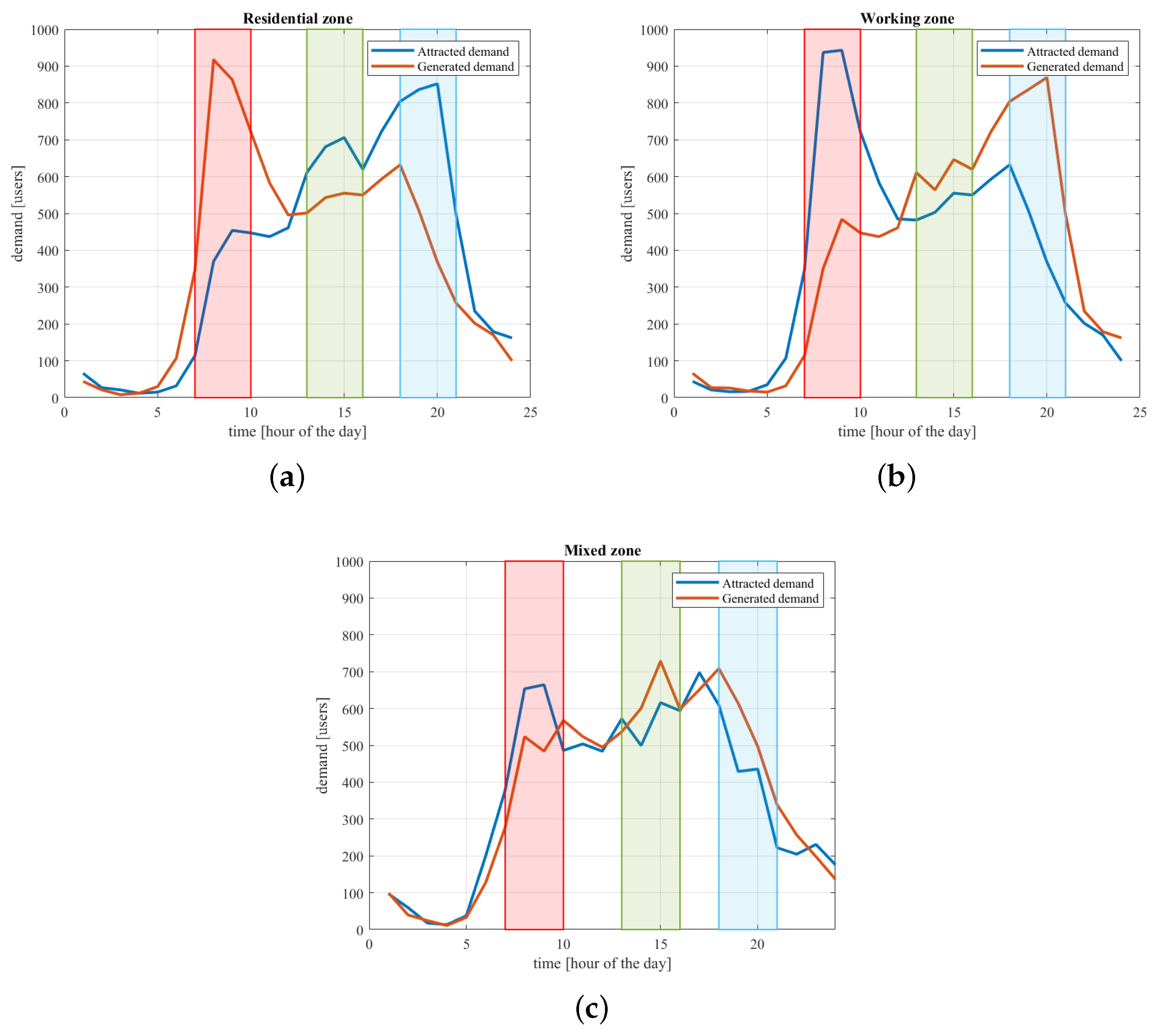
• in mainly residential zones (i.e., zones with a high density of housing), the generated demand is greater than the attracted demand—i.e., $D_{z·}^{kt}\gg D_{·z}^{kt}$—in the morning, since people leave their houses to reach workplaces, schools, or other economic activities. Conversely, attracted demand is greater than generated demand—i.e., $D_{·z}^{kt}\gg D_{z·}^{kt}$—in the afternoon and in the evening, when most people return home. During the other periods of the day, the generated and attracted demands are similar. An example of such differences is depicted in Figure 4a, where the hourly generated and attracted demands of a mainly residential zone are represented for a whole day.
• in mainly working areas (i.e., zones with a high density of workplaces), the attracted demand is greater than the generated demand—i.e., $D_{·z}^{kt}\gg D_{z·}^{kt}$—in the morning when most of the people go to work, while the generated demand is greater than the attracted demand—i.e., $D_{z·}^{kt}\gg D_{·z}^{kt}$—in the afternoon and in the evening, when most of the people return to home. During the other periods of the day, the generated and attracted demands are similar. An example of such differences is depicted in Figure 4b, where the hourly generated and attracted demands of a mainly working zone are shown for a whole day.
• in mixed zones, there is not a clear difference between the generated and attracted demands, i.e., $D_{z·}^{kt}$ is overall comparable to $D_{·z}^{kt}$ at all hours of the day, as shown in the example of Figure 4c.

3.3. Mobility Demand Modal Split

As already mentioned, the mobility demand $D_{od}^{kt}$ collects all the user travel needs between two zones at a given time period and for a given trip purpose. Nevertheless, since the supply system generally provides different modal alternatives to satisfy the demand (e.g., cars, public transport, pedestrians, etc.), it is common practice to split the demand $D_{od}^{kt}$ into contributions on the basis of the available transport modes such that ($o,d=1,2,\dots ,N;t=1,2,\dots ,T;k=1,2,\dots ,K$):

$$D_{od}^{kt}=\sum _{\ell =1}^L{D}_{od}^{kt\ell },$$

(3)

where L is the total number of available transport modes, and $D_{od}^{kt\ell }$ is the number of users travelling with transport mode ℓ ($\ell =1,2,\dots ,L$). The demand decomposition in (3) is widely known and used in the transportation engineering literature and can be achieved via specific models and/or surveys [8].

Similar decompositions can also be applied to the generated and attracted demands in (1) and (2), respectively. With these decompositions, it is possible to compute the demand generated and attracted by a generic zone z in the time unit t for the purpose k and with the transport alternative ℓ, namely, $D_{z·}^{kt\ell }$ and $D_{·z}^{kt\ell }$.

This modal decomposition can provide more insights regarding the activities performed in a certain zone.

In fact, there may be a correlation between the transport alternative and the trip purpose: for example, a peak of the generated demand for public transport in the early afternoon suggests the presence of schools in the zone (e.g., young students, who generally do not own a driving licence, come back home after school). Conversely, an evening peak of generated demand for both private vehicles and public transport may suggest a high density of offices or factories. As a further example, a high level of attracted or generated demand regarding freight-related modes (i.e., light or heavy trucks) can suggest the presence of productive activities (e.g., factories) or shops in a zone.

4. Materials and Methods

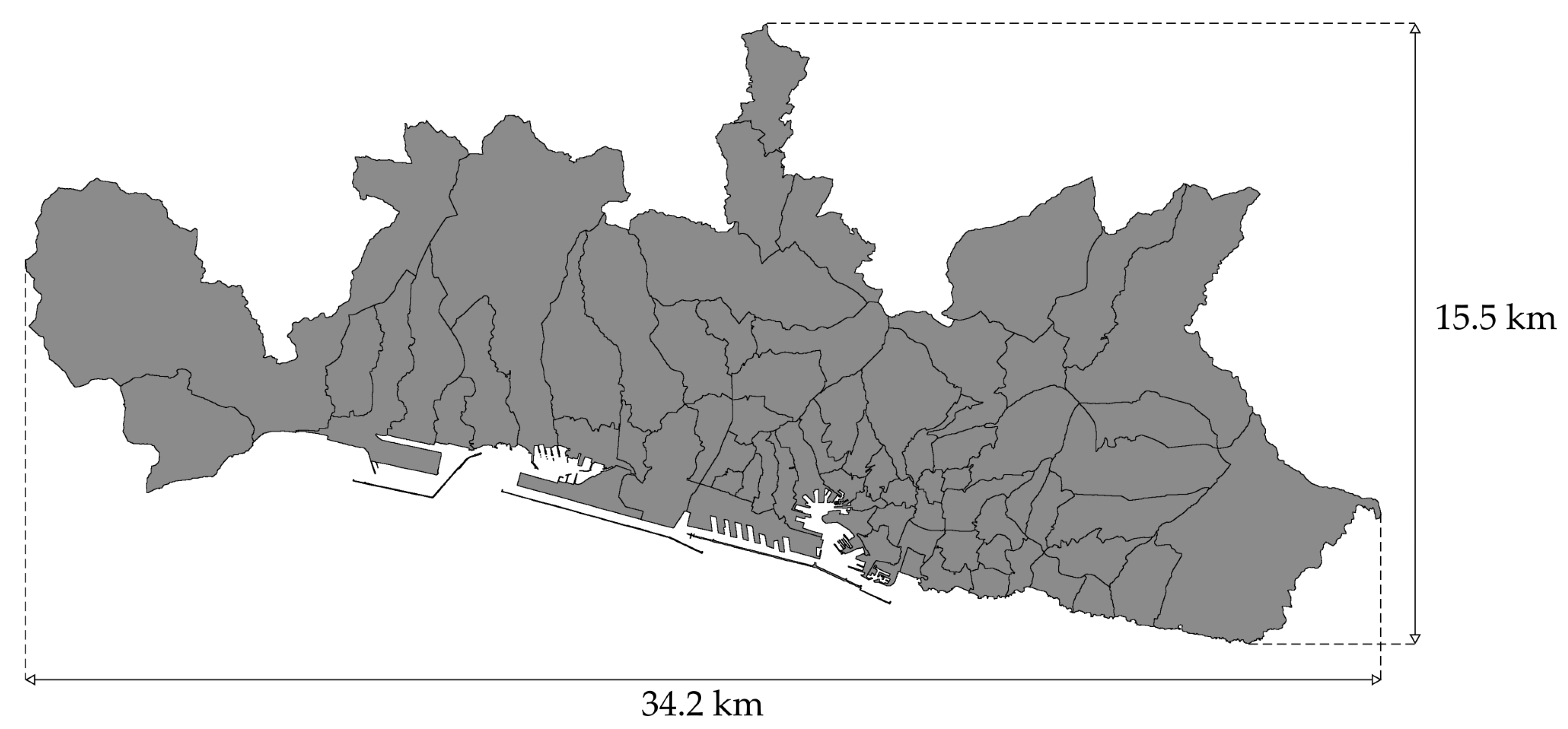
4.1. Case Study

The Italian city of Genoa, together with its surrounding area, is chosen as a case study. Both mobility demand data and high-resolution remotely sensed imagery are available for the present study. Genoa is located in northern Italy, and is the main urban area of the Liguria Region and the sixth largest city in Italy. It has a population of ≈585,000 inhabitants (https://dati.comune.genova.it/sites/default/files/EPR56U%202016.csv—in Italian, accessed on 25 April 2022), which increases to ≈850,000 when considering the whole metropolitan area (https://demo.istat.it/ricostruzione/dati/PopolazioneEta-Territorio-Province.zip—in Italian, accessed on 25 April 2022). The city, which is visible in the Sentinel-2 image in Figure 5 (false colour composite), spreads over a narrow and mainly hilly area of approximately 240 ${\mathrm{km}}^2$ between the Ligurian Sea and the Appennini Mountains; in particular, it stretches for more than 30 $\mathrm{km}$ along the coast and for over 10 $\mathrm{km}$ from the coast towards the north along the two valleys of the Polcevera and Bisagno Rivers. Historically, the current city of Genoa results from the unification of different towns and villages that, in 1926, became neighbourhoods of the city. For these reasons, Genoa presents a very articulated and differentiated urban fabric with different centralised locations acting as mobility generators and attractors. Its port is one of the most important of the Mediterranean Sea and characterises a relevant portion of the local economy influencing the urban structure and the location of different economic activities.

The significance of the urban area of Genoa, its articulated fabric, and the coexistence of different land-use typologies are among the reasons why this city has been adopted as the case study in the present work. A further reason is associated with the ground truth. In general terms, the ground truth for urban land-use mapping, to be used for validating the output classification results and for training supervised approaches, requires prior knowledge regarding the zones of the city, their districts, and the activities performed therein. In the considered case study, this ground truth could be collected thanks to the knowledge the authors have of the city of Genoa and of its current development. As detailed in Section 5, the ground truth on the urban land use of each neighbourhood of Genoa is used in the present study to train and validate the proposed methodologies.

The input remote sensing data used in the case study are given by a Copernicus Sentinel-2 multispectral image with a spatial resolution of 10 m and with four spectral channels (blue, green, red, and near infrared; see Figure 5).

The mobility demand data refer to a set of $N=71$ OD zones in which the territory of the municipality of Genoa is divided (see Figure 2) and to the related OD matrices (https://dati.comune.genova.it/dataset/matrici-origine-destinazione-spostamenti-e-viaggi—in Italian, accessed on 25 April 2022) that, coherently, have size $71\times 71$. More specifically, in terms of time period, data are available for $T=2$ time intervals, i.e., the morning peak hours (6:30 a.m. ÷ 9:00 a.m.) and the evening peak hours (5:30 p.m. ÷ 8:00 p.m.). For each time period, aggregated data are available for $L=3$ transport alternatives: the private mode (i.e., the sum over cars and motorcycles), the urban public transport (i.e., the sum over bus and urban metro rail), and the freight-related mode (i.e., the sum of medium and heavy trucks). Furthermore, for each time period and each transport alternative, data are available for $K=3$ trip purposes: “go to work/school”, “return home”, and “occasional”. In addition, the mobility demand attracted and generated by the surrounding area of Genoa, which can be thought of as an external zone, has been added to the result with the aim of also considering the trips that start or end outside the city.

Therefore, in summary, $T·L·K=18$ OD matrices $D^{kt\ell }$ are available. From each matrix and for each zone z ($z=1,2,\dots ,N=71$), the generated and attracted demands $D_{·z}^{kt\ell }$ and $D_{z·}^{kt\ell }$ are calculated and used as mobility demand features in the proposed approach (see next section). Accordingly, 36 mobility demand features are associated with each zone.

4.2. Multimodal Decision Fusion of Remote Sensing and Mobility Demand Data

A block diagram of the two proposed methodologies is depicted in Figure 6, where the relations between the pixelwise decision-fusion approach and the region-based Markovian approach are highlighted. The input data sources and the output of each methodology are also shown in this figure.

Let focus first on the proposed pixelwise fusion method. The zones to which the OD matrix corresponds are generally regions of an urban area and of the surrounding territory. Given the aforementioned remote sensing image of the same urban area, let $\mathcal{I}$ be the pixel lattice and ${\mathit{r}}_i$ be the feature vector extracted from the remote sensing image on pixel $i\in \mathcal{I}$. The OD zones correspond to N disjoint subsets ${\mathcal{Z}}_1,{\mathcal{Z}}_2,\dots ,{\mathcal{Z}}_N$ of the pixel lattice (${\mathcal{Z}}_n\subset \mathcal{I},{\mathcal{Z}}_m\cap {\mathcal{Z}}_n=\varnothing$ for $m,n=1,2,\dots ,N,m\ne n$). Let

$$\mathcal{Z}=\bigcup _{n=1}^N{\mathcal{Z}}_n$$

(4)

be the set of pixels enclosed in all OD zones. On the one hand, each zone ${\mathcal{Z}}_n$ usually corresponds to a city neighbourhood or a collection of neighbourhoods and is assumed to be administratively homogeneous. It corresponds to a portion of the urban cover in the scene and may generally also include other land covers in the peri-urban area (e.g., forestland, grassland, agricultural land at the outskirts of the city). On the other hand, the OD zones do not generally cover the entire imaged scene, which may generally correspond to a larger region surrounding the considered city, i.e., $\mathcal{Z}\subset \mathcal{I}$.

For the nth zone ($n=1,2,\dots ,N$), let ${\mathit{t}}_n$ be the vector gathering the mobility-generated demand flow and attracted demand flow for all purposes and all time units, as defined in (1) and (2) and discriminated for the transport modes as in (3). ${\mathit{t}}_n$ collects the quantities $D_{·n}^{kt\ell }$ and $D_{n·}^{kt\ell }$ across all trip purposes $k\in \{1,2,\dots ,K\}$, all time units $t\in \{1,2,\dots ,T\}$, and all modalities $\ell \in \{1,2,\dots ,L\}$. It represents a feature vector extracted from transport demand data on the nth zone ($n=1,2,\dots ,N$). As anticipated in the previous section, in the case of the considered case study of the city of Genoa, it is a 36-dimensional vector.

Let $\mathsf{\Omega }$ be the set of classes to be discriminated. We assume that it can be partitioned as $\mathsf{\Omega }=\mathsf{\Psi }\cup \overline{\mathsf{\Psi }}$, where $\mathsf{\Psi }$ includes urban land-use classes (e.g., “residential”, “working”, “commercial”) and $\overline{\mathsf{\Psi }}$ includes the additional (nonurban) land covers that are present in the imaged scene (e.g., water bodies, forestland, agricultural land). In this regard, the subset $\mathsf{\Psi }$ of classes collectively corresponds to the urban cover as a whole, and its elements are the individual urban land uses in the scene. In contrast, the subset $\overline{\mathsf{\Psi }}$ encompasses the other land covers in the considered urban and peri-urban areas. Given these different semantics, the two subsets of classes are meant to be disjoint, i.e., $\mathsf{\Psi }\cap \overline{\mathsf{\Psi }}=\varnothing$.

If $i\in \mathcal{Z}$ is a pixel within the overall area of the OD zones, let ${\nu }_i$ be the index of the corresponding zone, i.e., ${\nu }_i=n$ if and only if $i\in {\mathcal{Z}}_n$. Accordingly, the vector ${\mathit{x}}_i=[{\mathit{r}}_i,{\mathit{t}}_{{\nu }_i}]$ collects all features that are associated with pixel $i\in \mathcal{Z}$, including those extracted on pixel i from the input remote sensing image (${\mathit{r}}_i$) and those computed from the transport demand data on the zone including pixel i (${\mathit{t}}_{{\nu }_i}$). For a pixel outside the OD zones ($i\in \mathcal{I}\backslash \mathcal{Z}$), only remote sensing-derived features are available, and we set ${\mathit{x}}_i={\mathit{r}}_i$.

Let $y_i\in \mathsf{\Omega }$ be the class label of pixel $i\in \mathcal{I}$. First, we note that, in the case of a pixel i within the OD zones (i.e., $i\in \mathcal{Z}$) and of an urban land-use class (i.e., $y_i\in \mathsf{\Psi }$), the posterior probability $P\left(y_i\right|{\mathit{x}}_i)$, which is conditioned on all available—remote sensing and transport—features, can be expressed as:

$$P\left(y_i\right|{\mathit{x}}_i)=P(y_i,\mathsf{\Psi }|{\mathit{x}}_i)=P\left(y_i\right|\mathsf{\Psi },{\mathit{x}}_i)P\left(\mathsf{\Psi }\right|{\mathit{x}}_i).$$

(5)

In this framework, the proposed multimodal decision fusion approach is based on the following conditional independence assumptions:

$$\begin{array}{cc}\hfill P\left(y_i\right|\mathsf{\Psi },{\mathit{x}}_i)=P\left(y_i\right|\mathsf{\Psi },{\mathit{t}}_{{\nu }_i})& \forall i\in \mathcal{Z},y_i\in \mathsf{\Psi }\hfill \end{array}$$

(6a)

$$\begin{array}{cc}\hfill P\left(\mathsf{\Psi }\right|{\mathit{x}}_i)=P\left(\mathsf{\Psi }\right|{\mathit{r}}_i)& \forall i\in \mathcal{I}\hfill \end{array}$$

(6b)

$$\begin{array}{cc}\hfill P\left(y_i\right|{\mathit{x}}_i)=P\left(y_i\right|{\mathit{r}}_i)& \forall i\in \mathcal{I},y_i\in \overline{\mathsf{\Psi }}\hfill \end{array}$$

(6c)

Assumptions (6b) and (6c) imply that the membership of a pixel to the urban cover as a whole ($\mathsf{\Psi }$; see Assumption (6b)) or to the individual land-cover classes in $\overline{\mathsf{\Psi }}$ (see Assumption (6c)) is estimated according to the remote sensing features and regardless of mobility features. The rationale is that transport data convey information on how people move across the urban area, which is related to the use of the various city neighbourhoods. In contrast, transport demand features do not bear a relevant dependence on classes that are not associated with urban land use, such as the land-cover categories in $\overline{\mathsf{\Psi }}$. Accordingly, these land-cover classes, including the urban cover as a whole, are spatially discriminated only on the basis of the features extracted from remote sensing data.

Assumption (6a) indicates that, given the membership to the urban cover as a whole, the specific land use is determined based on the mobility-related features. On the one hand, as mentioned above, transport demand features are expected to be informative with respect to the discrimination of the use of a certain portion of the city territory. Remote sensing features generally also contribute to this discrimination in areas whose land use implies a well-defined spatial structure of the urban fabric and its buildings (e.g., presence of a large industrial complex). On the other hand, in portions of the urban areas whose use does not yield a peculiar spatial behaviour of the image, features extracted from the remote sensing data often do not strongly contribute to urban land use discrimination (e.g., in the case of city centre buildings that may correspond to both offices and residential houses). In this framework, Assumption (6a) plays the role of a simplifying hypothesis, under which the discrimination of urban land-use classes inside the urban cover is addressed by focusing only on the transport data.

Given the aforementioned assumptions, we can distinguish the three following cases in the modelling of the pixelwise posterior distribution:

• In the case of a pixel located within the OD zones (i.e., $i\in \mathcal{Z}$) and of an urban land-use class (i.e., $y_i\in \mathsf{\Psi }$), plugging Assumptions (6a) and (6b) in (5) yields:

  $$P\left(y_i\right|{\mathit{x}}_i)=P\left(y_i\right|\mathsf{\Psi },{\mathit{t}}_{{\nu }_i})P\left(\mathsf{\Psi }\right|{\mathit{r}}_i).$$

  (7)
  In this case, the pixelwise posterior of each urban land-use class is decomposed as the product of two terms, associated with the probability $P\left(\mathsf{\Psi }\right|{\mathit{r}}_i)$ of the urban cover as a whole, given the remote sensing observations, and with the probability $P\left(y_i\right|\mathsf{\Psi },{\mathit{t}}_{{\nu }_i})$ of the urban land-use class, given the transport features and the membership to the urban cover.
• In the case of a land-cover class ($y_i\in \overline{\mathsf{\Psi }}$) and of an arbitrary pixel ($i\in \mathcal{I}$), Assumption (6c) implies $P\left(y_i\right|{\mathit{x}}_i)=P\left(y_i\right|{\mathit{r}}_i)$.
• In the case of a pixel located outside the OD zones (i.e., $i\in \mathcal{I}\backslash \mathcal{Z}$), only remote sensing features are available (${\mathit{x}}_i={\mathit{r}}_i$); therefore, $P\left(y_i\right|{\mathit{x}}_i)=P\left(y_i\right|{\mathit{r}}_i)$ again.

Summing up the three cases, the following decision fusion model is defined to combine remote sensing and transport demand features for the classification of urban land-use and land-cover classes (see Figure 6):

$$\begin{array}{c}\hfill P\left(y_i\right|{\mathit{x}}_i)=\left\{\begin{array}{cc}P\left(y_i\right|\mathsf{\Psi },{\mathit{t}}_{{\nu }_i})P\left(\mathsf{\Psi }\right|{\mathit{r}}_i)\hfill & \mathrm{for}i\in \mathcal{Z}\mathrm{and}{y}_i\in \mathsf{\Psi }\hfill \\ P\left(y_i\right|{\mathit{r}}_i)\hfill & \mathrm{otherwise}.\hfill \end{array}\right.\end{array}$$

(8)

Based on the maximum a-posteriori (MAP) criterion, the first proposed multimodal fusion method assigns each pixel the class label that maximises the fused posterior in (8) (see Figure 6). The partial posteriors $P\left(y_i\right|{\mathit{r}}_i)$ and $P\left(y_i\right|\mathsf{\Psi },{\mathit{t}}_{{\nu }_i})$, conditioned to remote sensing and mobility observations, respectively, are estimated in a supervised manner using the random forest (RF) algorithm. Random forest is a well-known ensemble learning technique that defines a stochastic ensemble of decision trees, trained using bagging and random feature selection such that their outputs are as independent as possible [42]. In the proposed method, random forest is adopted thanks to its fully nonparametric formulation—which makes it possible to apply it to input features with arbitrary distribution—to its robustness to overfitting, and to its low computational burden [42].

For training the proposed supervised approach, two sources of ground truth data are assumed available:

(a)

a ground truth map regarding the individual land-cover classes in $\overline{\mathsf{\Psi }}$ and the urban land cover;

(b)

a subset of the zones ${\mathcal{Z}}_1,{\mathcal{Z}}_2,\dots ,{\mathcal{Z}}_N$ belonging to each urban land-use class.

On the one hand, the ground truth map in (a) indicates training pixels for each individual land-cover class in $\overline{\mathsf{\Psi }}$ as well as for the urban cover $\mathsf{\Psi }$. The latter is considered in this training map as a whole, i.e., examples of the individual urban land-use classes on a pixelwise basis are not necessary in the proposed method. On the other hand, the ground truth for the urban land-use classes in (b) is defined in terms of OD zones, i.e., the proposed method requires input training information about the land use only at the semantic level of city neighbourhoods (or collections of neighbourhoods).

We note that, outside the OD zones (i.e., for $i\in \mathcal{I}\backslash \mathcal{Z}$), no transport features are defined and, based on (8), we can compute both $P\left(y_i\right|{\mathit{r}}_i)$ for each land-cover class $y_i\in \overline{\mathsf{\Psi }}$ and $P\left(\mathsf{\Psi }\right|{\mathit{r}}_i)$. Therefore, the proposed method assigns such a pixel i either to one of the land-cover classes or to the urban cover as a whole but will not assign it to one of the urban land-use classes. This is consistent with the fact that a pixel outside the OD zones is meant to be outside the city and the related peri-urban region, and, accordingly, an urban land use would be undefined.

4.3. Markovian Region-Based Multimodal Fusion of Remote Sensing and Mobility Demand Data

Motivated by the intrinsic region-based spatial structure of the OD zones, the second proposed fusion method leverages the spatial-contextual modelling capabilities of MRF models [11,43]. MRFs are a powerful family of stochastic models for image data in Bayesian image analysis [43,44]. They have been successfully applied for a long time in remote sensing for image classification and segmentation [24,45,46,47,48,49,50], object-based and region-based image analysis [10,51,52], cloud detection [53,54], and change detection [55,56,57]. They represent a multi-dimensional generalisation of Markov chains and, in the case of 2D images, are defined in terms of a Markovianity property on the two-dimensional pixel lattice with respect to a given neighbourhood system [11,43,44].

In principle, each pixel depends on all the other pixels that make up an image. However, a Bayesian image-analysis problem formalised with such a global dependence would be computationally intractable in general. Taking advantage of the Markovian property, it is possible to restrict the probability distribution of a pixel conditioned to the whole image to the distribution conditioned only to a limited number of pixels in its surroundings [11]. However, regardless of this formulation in terms of local distributions, an MRF model also provides a full characterisation of the global (image-wise) distribution. Through the Hammersley–Clifford theorem, MRFs can be proven to correspond to global probabilistic models for the joint distribution of the image data (namely, Gibbs distribution models) [44], thus leading to a computationally tractable formulation of the Bayesian MAP decision criterion in terms of an appropriate “energy function” [11,43].

Specifically, let $\mathcal{X}={\left\{{\mathit{x}}_i\right\}}_{i\in \mathcal{I}}$ and $\mathcal{Y}={\left\{y_i\right\}}_{i\in \mathcal{I}}$ be the two-dimensional random fields of the feature vectors and the class labels, respectively. For classification purposes, an MRF is typically used as a model for the prior distribution of the random field $\mathcal{Y}$ of the class labels [10,11]. $\mathcal{Y}$ is said to be an MRF if its joint distribution $P\left(\mathcal{Y}\right)$ is strictly positive and if the following Markovianity property holds:

$$P\left(y_i\right|y_j,j\ne i)=P\left(y_i\right|y_j,j\sim i)\forall i\in \mathcal{I},$$

(9)

where $i\sim j$ indicates that pixels i and j are neighbours with respect to a predefined neighbourhood system [11,43]. While the strict positivity is basically a technical assumption, the Markovianity represents the core of the MRF notion. A well-known result of the MRF theory is that, if $\mathcal{Y}$ is an MRF, then, under suitable conditional-independence assumptions, the maximisation of the global posterior distribution $P\left(\mathcal{Y}\right|\mathcal{X})$ is equivalent to the minimisation of an energy function $U\left(\mathcal{Y}\right|\mathcal{X})$ that characterises both pixelwise and spatial-contextual information and is defined locally according to the aforementioned neighbourhood system. Indeed, the relationship $P\left(\mathcal{Y}\right|\mathcal{X})\propto exp[-U\left(\mathcal{Y}\right|\mathcal{X}\left)\right]$ holds between the global posterior distribution and the energy [11,44]. Details on MRF modelling and their use in VHR remote sensing image classification can be found in [10,11].

In this framework, the second proposed method generalises the MRF model in [10], which allows spatial information associated with both the local context and the membership to homogeneous regions to be fused together, by integrating it with the mobility features and their spatial zonization. Region-based and object-based models are usually employed to discriminate classes that exhibit a well-defined geometrical structure [52,58]. They incorporate information associated with the output of an image segmentation result and with the corresponding segments. Region-based MRFs directly model spatial information associated not only with a local neighbourhood but also with image regions, which are generally larger (possibly much larger) than the neighbourhood and which capture long-range spatial dependencies [10,59].

In particular, multiscale region-based MRFs also integrate multiscale information by using segmentation results corresponding to different spatial scales or resolutions [60]. In this case, one leverages the capabilities of MRFs to perform data fusion in order to exploit the multiscale information for classification purposes [10,61]. Given an image to be classified, a multiscale segmentation method is applied to generate a collection of segmentation maps, including coarse- and fine-scale maps. At finer scales, small spatial details can be appreciated but noise can have a significant impact, whereas at coarser scales, only large image structures and regions are preserved but with a strong immunity to noise [10]. Each segmentation map is considered as a distinct information source, formalising the classification task as a data fusion problem [10]. Consistently with the MRF approach to data fusion [61], the energy $U\left(\mathcal{Y}\right|\mathcal{X})$ of a multiscale region-based MRF is expressed as a linear combination of energy contributions related to the individual pixels (pixelwise terms) and to the spatial information contained both in the neighbourhood of each pixel and in the segmentation map at each scale [10,61].

In the second proposed method, this approach is further generalised by integrating in the MRF model spatial-geometrical structure given not only by a multiscale segmentation result but also by the zonization of the mobility data. Let Q segmentation maps, corresponding to Q different spatial scales, be computed from the input remote sensing image, and let $s_{iq}$ be the segment label of pixel $i\in \mathcal{I}$ in the qth map ($q=1,2,\dots ,Q$). We define the following MRF energy (see Figure 6):

$$\begin{array}{c}U\left(\mathcal{Y}\right|\mathcal{X},\mathcal{S},\mathcal{N})=-\sum _{i\in \mathcal{I}}lnP\left(y_i\right|{\mathit{x}}_i)-\sum _{i\in \mathcal{I}}\sum _{q=1}^Q{\alpha }_{q}lnP\left(s_{iq}\right|y_i)+\hfill \\ \hfill -\beta \sum _{i\in \mathcal{Z}}lnP\left({\nu }_i\right|y_i)-\gamma \sum _{i\sim j}\delta (y_i,y_j),\end{array}$$

(10)

where $\delta (·)$ is the Kronecker impulse, ${\alpha }_q$ ($q=1,2,\dots ,Q$), $\beta ,\gamma$ are positive weight coefficients, $\mathcal{S}=\{s_{iq}:i\in \mathcal{I},q=1,2,\dots ,Q\}$ is the random field collecting all segment labels in the Q segmentation maps, and $\mathcal{N}={\left\{{\nu }_i\right\}}_{i\in \mathcal{Z}}$ analogously collects the zone indices of all pixels in $\mathcal{Z}$. The second-order neighbourhood is used, i.e., $i\sim j$ if and only if j is one of the eight pixels surrounding pixel i (and vice versa) [11].

As in [10], energy contributions associated with the class-conditional distributions $P\left(s_{iq}\right|y_i)$ of the segment labels in the Q segmentation maps and with the local contextual Potts model (i.e., the well-known term $[-{\sum }_{i\sim j}\delta (y_i,y_j)]$ [11]) are included in the energy (10) (see Figure 6). As discussed above, the rationale of the terms associated with the Q segmentation maps in (10) is to incorporate multiscale information in the labelling process by extracting and using segmentation maps corresponding to Q spatial scales. In the terms $P\left(s_{iq}\right|y_i)$, segment labels are considered as features and allow a model of the relation between the classes and the multiscale segmentation maps to be integrated in the data fusion process [10]. The well-known Potts MRF model [11] favours the same labelling within homogeneous image regions.

In the proposed method, a further energy term associated with the OD zones and expressed in terms of the class-conditional distribution $P\left({\nu }_i\right|y_i)$ of the zone index is also integrated (see Figure 6). From a methodological point of view, this corresponds to defining and using for classification a composite stack of region maps, deriving both from the segmentation of the remote sensing image at coarse-to-fine scales and from the zonization associated with the OD data. Similar to the case of $P\left(s_{iq}\right|y_i)$, in the term $P\left({\nu }_i\right|y_i)$, the zone index ${\nu }_i$ plays the role of a further feature. This interpretation of $s_{iq}$ and ${\nu }_i$ as additional features in the classification process explains the notation $U\left(\mathcal{Y}\right|\mathcal{X},\mathcal{S},\mathcal{N})$ for the energy in (10). A pixelwise term associated with the fused posterior $P\left(y_i\right|{\mathit{x}}_i)$ in (8) is also included in the energy (10). This term is related to the probability that pixel i has label $y_i$ given the feature vector ${\mathit{x}}_i$, which includes remote-sensing and mobility demand data. The aforementioned composite stack of segmentation maps is semantically mixed since it includes Q maps computed from the input image data and one additional map derived from the OD zones. Accordingly, in the second proposed method, multimodal fusion of remote-sensing and transport-demand data are accomplished in terms not only of decision fusion, through the pixelwise energy contribution $[-lnP\left(y_i\right|{\mathit{x}}_i)]$, but also of the spatial information associated with both the remote sensing image and the OD zonization.

In the second developed technique, the algorithm in [62] is used to generate the Q segmentation maps (see Figure 6). It has been selected as a well-known approach for the segmentation of optical image data, which has proven successful in its combination with region-based MRF models in [10,51]. It is a graph-based region-merging algorithm and is parameterised by a parameter k that indirectly determines the scale of the extracted segments [62]. To generate the Q segmentation maps, the algorithm is separately run Q times with increasing values of k in a predefined range. Examples of the resulting segmentation output can be seen in the block diagram of Figure 6.

Since the region labels $s_{iq}$ and the zone index ${\nu }_i$ are discrete random variables, their class-conditional distributions $P\left(s_{iq}\right|y_i)$ ($q=1,2,\dots ,Q$) and $P\left({\nu }_i\right|y_i)$ are estimated through the corresponding relative frequencies on the classification map obtained by the first proposed method. For example, $P\{{\nu }_i=n|y_i=\omega \}$ is estimated as the relative frequency of the pixels that belong to zone ${\mathcal{Z}}_n$ ($n=1,2,\dots ,N$) amongst those that are assigned to class $\omega \in \mathsf{\Omega }$ by the first proposed method. Further details on the estimation of these distributions can be found in [10].

The weight parameters ${\alpha }_1,{\alpha }_2,\dots ,{\alpha }_Q,\beta$, and $\gamma$ are optimised by using the technique in [63]. Given a preliminary classification map, which is here the one generated by the first proposed method, this technique expresses the condition that the training samples are correctly classified by the minimum energy rule in terms of an overconditioned system of linear inequalities. The solution of this system is addressed using the least mean square error criterion, which, in turn, is numerically formulated through the iterative Ho–Kashyap algorithm [64]. Convergence in a finite number of steps is analytically guaranteed [64]. The energy function in (10) is minimised using the iterated conditional mode (ICM) algorithm (see Figure 6). ICM is a well-known iterative technique for the minimisation of MRF energies that is proven to converge to a local minimum and generally requires a short computation time. It is often an effective trade-off between classification accuracy and computational burden. Details can be found in [11]. In the second proposed method, ICM is initialised with the pixelwise classification result of the first developed technique.

Consistently with the previous works in [10,51], the random field model defined by the energy in (10) has been described as an MRF, rather than a conditional random field (CRF). This is due to the aforementioned interpretation of the segmentation labels $s_{iq}$ and the zone index ${\nu }_i$ as additional features or observations. From this perspective, $P\left(s_{iq}\right|y_i)$$(q=1,2,\dots ,Q)$ and $P\left({\nu }_i\right|y_i)$ are interpreted as the class-conditional distributions of those features, given the pixelwise class label $y_i$. However, the proposed contextual model can also be considered as a CRF [43,65]. The rationale is that the segment labels $s_{iq}$ are generated through the application of the segmentation algorithm in [62] to the input image, i.e., to the random field $\mathcal{X}$ of the observations. Therefore, they can be considered as functions $s_{iq}\left(\mathcal{X}\right)$. Under this interpretation, the pixelwise contributions $[-lnP\left(s_{iq}\right|y_i)]$ to the energy function of the proposed model would generally depend on the whole random field $\mathcal{X}$, a property that would qualify the model as a CRF [43,65]. Overall, given the two aforementioned possible interpretations, the random field associated with the second proposed method can be correctly referred to as either an MRF or a CRF. In the following, we will continue referring to it as an MRF, for the sake of consistency with the previous papers in [10,51].

We also recall that Markov chain random field (MCRF) models have recently been applied within Bayesian schemes for land-cover mapping [66,67,68,69] and updating [45,70]. In the MCRF solution, the spatial dependencies among nearest samples and the central random variable can be described by a probabilistic directed acyclic graph that conforms to a neighbourhood-based Bayesian network on spatial data. A first major difference between our proposed method—and MRF-based methods in general—and MCRFs is that the model employed in our paper represents a 2D generalisation of Markov chains, whereas an MCRF is actually a Markov chain. A second relevant difference regards their characteristics as probabilistic graphical models [65]. As mentioned above, an MCRF is based on a directed graph, a property that relates it to the area of Bayesian networks. On the contrary, from a graph-theoretic perspective, MRF models are based on undirected graphs [65].

5. Experimental Results

The two proposed multimodal fusion methods have been experimentally validated on the case study of the city of Genoa described in Section 4.1. Regarding the ground truth for the training and the testing, the urban land use associated with each of the 71 zones has been determined based on prior knowledge on the city structure and on the characteristics of its neighbourhoods within the urban territory. Three urban land-use classes have been identified, i.e., “residential”, “working”, and “mixed” (i.e., $\mathsf{\Psi }$ = {residential, working, mixed}). The “residential” class is associated with neighbourhoods with a well-defined housing vocation. The “working” class encompasses industrial, port, and office activities across the city, and “mixed” includes neighbourhoods in which both offices and housing are prominent. In this respect, the considered case study is particularly challenging, as the three land-use classes strongly overlap. In particular, the discrimination of the class “mixed” is expected to be especially difficult because this class is intrinsically characterised by a significant semantic overlapping with both the “residential” and “working” classes. Furthermore, in the mixed zones, there is not a clear difference between the generated and attracted mobility demands, thus making the discrimination of the land use of the area even more complicated. This characteristic of the case study derives from the spatial structure of the city and relates to the homogeneity criterion of the OD zonization, since several neighbourhoods of the city of Genoa truly correspond to mixed land use.

The ground truth for the urban land use of the 71 zones is shown in Figure 7a,b, which refer to the zones used for training the proposed approaches and for testing their accuracies, respectively (see Section 4.2). In particular, 35 zones (see Figure 7a) have been used to train a random forest classifier that estimates the posteriors $P\left(y_i\right|\mathsf{\Psi },{\mathit{t}}_{{\nu }_i})$ ($y_i\in \mathsf{\Psi }$) of the urban land-use classes, conditioned on the transport demand features, while the remaining 36 zones have been used for testing (see Figure 7b).

Furthermore, according to the characteristics of the region around Genoa, which is a port city on the Ligurian Sea and is mostly surrounded by forestland, the set of nonurban land-cover classes in the considered case study is $\overline{\mathsf{\Psi }}=\left\{\mathrm{vegetation},\mathrm{water}\mathrm{body}\right\}$. The training map for “vegetation”, “water body”, and “urban cover” is shown in Figure 8a. It has been used within the proposed techniques to train random forest for estimating $P\left(y_i\right|{\mathit{r}}_i)$ ($y_i\in \overline{\mathsf{\Psi }}$) and $P\left(\mathsf{\Psi }\right|{\mathit{r}}_i)$, i.e., the posteriors of “vegetated”, “water body”, and of the urban cover as a whole, given the remote sensing features. In particular, the multispectral channels of the input Sentinel-2 image have been used as remote sensing features in the application of the proposed fusion techniques. Similarly, Figure 8b shows the test map used in the quantitative assessment of the proposed algorithms. Since both methods assign each pixel a class label in the complete set of classes $\mathsf{\Omega }=\mathsf{\Psi }\cup \overline{\mathsf{\Psi }}$, both urban land-use and nonurban land-cover classes are present in this test map.

First, as a preliminary result, the outcome of the classification of the individual OD zones among the three urban land-use classes is depicted in Figure 9a. For the sake of comparison, the complete ground truth is shown in Figure 9b. Here, it is worth noting that all the pixels belonging to the same zone ${\mathcal{Z}}_n$ share the same transport-demand features and consequently the same posterior distribution conditioned on transport data (i.e., $P\left(y_i\right|\mathsf{\Psi },{\mathit{t}}_n)$ depends on the zone ${\mathcal{Z}}_n$ and is constant over all pixels $i\in {\mathcal{Z}}_n$ enclosed within it). The producer and user accuracies (PAs and UAs) of the three urban land-use classes in this classification result, with respect to the test map in Figure 7b, are reported in

Table 1. Producer, user, overall, average accuracies and Cohen’s $\kappa$ of OD zone classification based on mobility-demand features. Since the number of test zones is 36, the accuracy values are discretised to multiples of 2.5% and only two digits are reported for $\kappa$.

	Residential ■	Mixed ■	Working ■
Producer accuracy (%)	87.5	80.0	100
User accuracy (%)	87.5	85.0	85.0
Overall accuracy (%)	85.0
Average accuracy (%)	90.0
Cohen’s $\kappa$	0.78

, together with the overall accuracy (OA), the average accuracy (AA), and Cohen’s $\kappa$ statistics.

Then, the classification maps generated by the proposed pixelwise and Markovian fusion methodologies are shown in Figure 10. Their quantitative assessment in terms of PA and UA values with respect to the test map in Figure 8b is presented in

Table 2. Producer, user, overall, average accuracies and Cohen’s $\kappa$ of the proposed methods and of the compared approaches: (i) classification of only the spectral channels; (ii) soft-majority voting applied to the pixelwise posteriors estimated from only the spectral channels; (iii) classification in the stacked feature space of spectral channels, NDVI, and texture features; and (iv) soft-majority voting applied to the pixelwise posteriors estimated in the stacked feature space.

	Producer Accuracy (%)
	Residential ■	Mixed ■	Working ■	Vegetation ■	Water Body ■
(i)	34.54	45.77	23.28	41.90	99.96
(ii)	36.37	46.62	19.58	51.36	99.99
(iii)	37.18	63.13	0	41.90	99.97
(iv)	28.49	55.22	17.22	51.36	99.99
Proposed pixelwise	90.42	87.07	77.58	42.94	99.99
Proposed MRF region-based	70.71	88.69	99.99	99.23	100
	User Accuracy (%)
	residential ■	mixed ■	working ■	vegetation ■	water body ■
(i)	20.33	17.73	27.23	99.56	99.97
(ii)	22.68	24.75	28.30	99.81	99.99
(iii)	38.48	29.67	0	99.56	99.97
(iv)	9.13	16.61	46.31	99.81	99.99
Proposed pixelwise	39.29	53.96	77.28	99.55	100
Proposed MRF region-based	88.18	84.68	76.04	100	100
	Overall Accuracy (%)		Average Accuracy (%)		Cohen’s $\kappa$
(i)	50.12		49.09		0.3820
(ii)	54.76		48.44		0.4274
(iii)	52.82		50.79		0.4138
(iv)	49.32		50.46		0.3856
Proposed pixelwise	70.25		79.60		0.6286
Proposed MRF region-based	89.98		91.72		0.8706

. To evaluate the usefulness of mobility demand data, the results of the proposed methods were compared to those of classical baseline strategies for land-use and land-cover mapping based on the classification of spectral and textural features (without transport demand data):

(i)

Pixelwise classification of the remotely sensed image, using its multispectral channels as features—This is meant as a consolidated baseline for land-cover mapping. Random forest was chosen as a well-known benchmark classifier and was trained to discriminate all the classes in $\mathsf{\Omega }$. The training samples for “vegetation” and “water bodies” are shown in Figure 8. Regarding the urban land-use classes, pixelwise training samples were obtained through the spatial intersection between the training regions of “urban cover” in Figure 8a and the training OD zones in Figure 7a;

(ii)

Pixelwise classification using not only the multispectral channels but also additional features including the normalised difference vegetation index (NDVI) and texture features—Random forest has been used in this case as well, thanks to its fully nonparametric formulation that allows the application to heterogeneous input features. Texture analysis is conducted using the well-known first-order histogram (FOH) and grey-level cooccurrence matrix (GLCM) approaches [71,72]. The FOH variance and GLCM contrast and variance features were extracted from all channels of the input Sentinel-2 image. Preliminary experiments, not reported for brevity, have been performed to tune the parameters of the FOH and GLCM texture analysis algorithms to optimise the classification results. Texture features have been found informative in the literature of land-use mapping from remote sensing imagery (e.g., [73,74]), and this experiment is aimed at discussing the behaviour of the proposed methods compared to a traditional approach to land-use classification from EO data. The training set used for this experiment is the same as in (i);

(iii)

Soft-majority voting on the posteriors computed by classifier (i)—In this case, for each OD zone and each urban land-use class, first, the average of the pixelwise posteriors predicted by random forest in (i) is computed. Then, each pixel of the zone is assigned by applying the MAP rule with the averaged posteriors of the urban land-use classes and with the pixelwise posteriors of the nonurban land-cover classes. Averaging is applied only to the posteriors of the urban land-use classes (and not to those of “vegetation” and “water bodies”) to take into account that the zonization is associated with the urban mobility and generally not with other land covers. The aim of this experiment is to appreciate the possible contribution of the spatial discretization associated with the OD zones within a traditional classification scheme as in (i), in comparison to the developed techniques in which mobility-related information is exploited in terms both of spatial structure and of transport demand features;

(iv)

Soft-majority voting as in (iii), applied here to the pixelwise posteriors obtained in (ii) from input spectral channels and additional features—While the rationale of this experiment is similar to that of (iii), here, the focus is on evaluating the possible benefit of combining a traditional land-use classification strategy with the spatial structure of mobility demand data.

The values of PA, UA, OA, AA, and $\kappa$ obtained by these benchmark approaches are shown in Table 2.

6. Discussion

Regarding the preliminary result in Figure 9a, which is about the classification of the OD zones among the urban land-use classes based on the transport demand features, a visual comparison with the ground truth in Figure 9b indicates that only a few zones are misclassified. It is worth noting that they are all related to the “mixed” class. Two mixed zones are erroneously classified as “residential”, and a third zone is labelled as “working”, whereas two residential zones are assigned to “mixed”. On the one hand, as discussed in Section 5, this is an expected type of error due to the semantics of the “mixed” class, which corresponds by definition to city neighbourhoods in which housing and working activities coexist significantly. On the other hand, in the result of Figure 9a, there is no confusion between the “residential” and “working” classes. This visual analysis is confirmed quantitatively by the high values of PA and UA for the three classes and of OA, AA, and $\kappa$ (see Table 1). These results suggest the relevance of transport-demand data from the viewpoint of the discrimination of urban land use and the effectiveness of the features computed from these data on each OD zone. This is consistent with the relation between mobility demand from/to a city neighbourhood and the land use in that neighbourhood and confirms the opportunity to exploit transport engineering data within urban land-use mapping from satellite imagery.

These comments are also confirmed by a qualitative analysis of the maps generated by the two proposed methods (see Figure 10), in which the land-cover and urban land-use classes appear to be well distinguished. A quantitative assessment in terms of PA and UA values with respect to the test set (see Table 2) confirms the effectiveness of the proposed approaches. In particular, in the discrimination of the three urban land-use classes, the pixelwise multimodal fusion method obtained rather high values of PA ranging approximately from $78\%$ to $90\%$, although the values of UA were lower in the cases of “residential” and “mixed”. The proposed Markovian region-based fusion technique obtained high values of both PA and UA on all three classes. The values of OA, AA, and $\kappa$ achieved by the two proposed methods confirmed the accuracy of their maps and especially of the output of the Markovian region-based fusion technique. These results suggest the potential of mobility demand data in conjunction with remote sensing imagery for mapping urban land use and the effectiveness of the proposed probabilistic approach to address this multimodal fusion task.

In particular, the test-set results indicate the improvement obtained by the proposed MRF-based technique, which also incorporates spatial-contextual and multiscale information in the mapping process, compared to the pixelwise decision fusion algorithm. A visual analysis of the corresponding classification maps (see Figure 10) indicates, as expected, that the use of the Markovian approach yields higher spatial smoothness than the output of the pixelwise fusion method. In the specific considered fusion problem, in which one of the two sources is inherently associated with a zonization, spatial information is also conveyed by the OD zones themselves. A case-specific example is shown in Figure 11, which focuses on a detail of the port of Genoa. Comparing the classification maps obtained by the pixelwise and Markovian methods (see Figure 11b,c, respectively), it is possible to note how the ships around the docks, which are outside the OD zones, are mostly labelled with the urban land-use class of the adjacent OD zones in the output of the MRF-based approach. Indeed, in terms of the semantics of the urban land-use classes, this is correct because ships are generators and attractors of mobility demand. More generally, the opportunity to address mobility/EO data fusion with different levels of spatial smoothness is generally a desired byproduct because it can be used to match the requirements of the specific urban application. For example, while the result of the Markovian fusion method is spatially more regular and clearly emphasises the land use of the various neighbourhoods, the result of the pixelwise fusion method allows to draw the attention to small-scale spatial features associated with urban vegetation.

It is worth noting that the pixels assigned to the urban land-use classes in Figure 10 tend to be spatially organised in connected regions. This is consistent with the aforementioned discretisation into the OD zones and with the semantics of the considered land-use classes. In particular, it can be noticed in Figure 10b that, among the effects of the contribution associated with the OD zones in the energy (10), it is favoured that pixels outside the zones are assigned to nonland-use classes. This is a desired behaviour because urban land-use semantics are defined only within the city area.

Indeed, the boundaries of the OD zones are determined by administrative criteria that consider the subdivision of the city into neighbourhoods, thus implicitly relating to land use but generally without taking land cover into account. Consistently, in the case of several zones of both maps in Figure 10—especially the zones at the outskirts of the city—a large portion of the zone territory is covered by vegetation. On the one hand, the administrative definition of these zones formally includes large portions of forestland. On the other hand, the proposed techniques correctly discriminate the portions of urban and vegetated cover within each zone and assign the former to the urban land-use classes.

The considered previous techniques for land-cover and land-use mapping obtained very high values of PA and UA for “water bodies” and of UA for “vegetation”, similar to the accuracies achieved by the proposed methods for these classes (see Table 2). This is an expected result, thanks to the consolidated capability of nonparametric supervised classifiers such as random forest in the application to such a land-cover mapping task [72]. However, in the case of the pixelwise classification using the spectral channels or the additional features, the discrimination of the urban land-use classes was quite poor. Majority aggregation over the OD zones led to improvements for “residential” and “working” but did not allow “mixed” zones to be distinguished. The proposed techniques obtained significantly more accurate discrimination of the urban land-use classes than the considered baseline approaches. This is also reflected in the values of OA, AA, and $\kappa$ of the proposed and comparison methods (see Table 2). These results confirm the challenge of distinguishing urban land use purely on the basis of remote-sensing imagery and further support the opportunity to fuse them with mobility demand data through the proposed methods. In particular, the comparison between the results of the developed algorithms and of the soft-majority approaches suggests that not only the spatial discretisation into the OD zones but also the transport demand features play an important role in the identification of the urban land use of the city neighbourhoods.

A visual analysis of the corresponding maps (see the details in Figure 12) also confirms these comments. Compared to the map generated by applying random forest only to the spectral channels (see Figure 12d), the results obtained in the stacked feature space including spectral channels, NDVI and texture descriptors (see Figure 12f), exhibits an improved spatial regularity, especially within the portion of the image associated with the urban fabric. This is explained by the use of spatial information through texture analysis. Nevertheless, in both maps, the discrimination among the urban land-use classes is also visually quite poor. In both cases, pixels drawn from the same city area and neighbourhood are assigned to different urban land-use classes, i.e., the land use of each area or neighbourhood is not recognised.

In the classification maps generated through soft-majority voting, on the OD zones, of the pixelwise posteriors predicted by random forest (see Figure 12e,g), the spatial structure partially reflects that of the OD zones. However, compared to the ground truth of the urban land use of the zones (see Figure 12b), the labelling obtained by the proposed approach (see Figure 12c, which focuses on the pixelwise decision fusion algorithm), is more accurate than the labelling yielded by soft-majority voting. This visually confirms the potential of the joint use of remote-sensing and mobility demand data—not only through the zonization but also through the OD matrix—and the effectiveness of the developed multimodal fusion approach. It is also worth noting that the ground truth in Figure 12b regards only the urban land-use classes (i.e., it is a crop of Figure 9b), whereas the portion of the scene in Figure 12a clearly also includes vegetated areas, which are correctly detected in the result of the proposed approach. We also recall that the considered soft-majority voting operates on the urban land-use classes but does not act on the pixels assigned to nonurban land covers in Figure 12d,f. In contrast, the developed approach performs a probabilistic decision fusion that, on each pixel, considers all classes in $\mathsf{\Omega }$.

As mentioned in Section 1, to the authors’ knowledge, this paper is the first one exploring the potential of the joint use of remote-sensing and mobility demand data in the framework of urban land-use and land-cover mapping. Therefore, comparison with state-of-the-art techniques using the same types of input data is not feasible. The most common case of combination of remote-sensing and ancillary data for land-use and land-cover mapping involves OSM and not mobility demand. Indeed, studies using the fusion of OSM and remote-sensing data confirm the advantages of integrating satellite imagery with complementary information. For example, in [19], their combination allowed for performing land-cover mapping of large-scale urban areas through ensemble learning techniques (e.g., random forest) in an efficient way. Similarly, in [26], OSM data were used to incorporate semantic information to the geographical objects extracted by a deep learning method in order to improve the results of urban scene classification in complex urban areas. On the one hand, a direct comparison between the results in these previous papers and those in the present work is hindered by the fact that different case studies and data sets were used. On the other hand, consistently with the results in these previous works, the experimental validation discussed in the present section has confirmed—in the case of the proposed methods and of the use of the OD matrix—that the integration of remote-sensing images with suitable ancillary data favours a more accurate land-use classification output than when only EO imagery is used. Furthermore, the proposed approaches, as compared to techniques based on the fusion of OSM and EO data, can explicitly benefit from measurements associated with mobility demand from/to the city districts, which, as discussed in Section 3, are intrinsically related to the land use in those districts.

7. Conclusions

In this paper, a probabilistic methodology for the multimodal fusion of remote-sensing imagery and transport-demand data has been developed to address the challenging task of urban land-use and land-cover mapping. The goal of this work was to investigate the potential of mobility demand data (namely, Origin-Destination matrix data) and of their joint use with EO images. Two novel techniques have been developed for this purpose. The first addresses the aforementioned multimodal fusion problem on a pixelwise probabilistic basis. The second one integrates this probabilistic framework and the spatial structure of the mobility data within a region-based multiscale Markov random field model.

The results of the experimental validation, conducted on a case study associated with the city of Genoa, Italy, suggest the capability of the proposed techniques to identify the classes corresponding to the main land covers and urban land uses (i.e., “residential”, “working”, and “mixed” areas). Both proposed methods obtained high accuracies in the discrimination of urban land-use classes, thus suggesting the effectiveness of the proposed approach in taking advantage of the two input sources of information.

In particular, the developed techniques obtained remarkably higher accuracies than previous approaches to land-use and land-cover mapping based only on remote-sensing data and considering spectral and textural features. These results indicate the usefulness of the integration of methodological contributions stemming from remote sensing and transport-system engineering in the framework of the complex task of land-use mapping in urban environments. Furthermore, the proposed methods more accurately discriminated land use compared to soft-majority approaches in which satellite imagery was jointly used only with the spatial discretization associated with transport data. This confirms the potential of the proposed techniques for the fusion of remote-sensing imagery with the Origin-Destination matrix—and not only with its associated spatial zonization.

A comparison between the two proposed algorithms confirms the relevance of MRF models in remote-sensing image analysis. While both developed techniques generated accurate classification maps, improved performance was achieved by the Markovian region-based method compared to the pixelwise decision-fusion algorithm. On the one hand, this is an expected result due to the modelling of spatial-contextual information performed by the proposed MRF. On the other hand, the specific proposed MRF model, in turn, benefits from multiple sources of information, including multiscale segmentation results extracted from the input EO image and the spatial zonization associated with the OD matrix. From this perspective, the experimental results suggest the effectiveness of the adopted fusion strategy that is aimed at taking advantage of the multimodal, multiscale, and spatial information conveyed by satellite and mobility datasets.

Thanks to the ever-increasing availability of up-to-date mobility demand data, the proposed methodologies could also be beneficial in spatial planning applications. First, their use at different times allows to analyse the temporal evolution and dynamics of an urban area, thus making land-use changes appreciable even where cadastral data have not been updated, yet. This, in turn, can pave the way for the planning and design of interventions on the transport supply (in terms of both infrastructure and services) capable of meeting the needs arising from the changes in the urban areas. In this respect, since the OD matrix of a given city is normally updated on a regular basis, a possibly useful extension of the proposed region-based Markovian approach could be a multitemporal generalisation [51]. This extension would fuse such multitemporal OD data with a corresponding satellite image time series (SITS) to determine the temporal evolution of urban land use. Moreover, updated urban land-use information extracted through the proposed approaches could also be exploited to plan medium- or long-term interventions on urban areas to balance transport demand (e.g., location of residence, workplace and economic activities) and reduce travel times, congestion, and pollution. In addition, the proposed methodologies could be scaled from an urban level to a wider level (e.g., regional level), to include entire conurbations and analyse the relationships between a city and the towns close to it, provided that satellite and OD matrix data are available.

The main limitation of the present study lies in the discretisation level of the OD zonization. On the one hand, this discretisation derives from the structure of the mobility demand in the considered urban area and consequently relates to the urban land use of the city districts. On the other hand, if this discretisation was spatially refined, then the number of “mixed” zones and their overlapping with the “working” and “residential” classes could possibly be reduced. This spatial refinement could be accomplished by, first, further discretising the available OD zones following the principles described in Section 3, and then, by appropriately expanding the OD matrices (i.e., increasing their dimension to the number of the newly created zones) [75]. Nevertheless, a subset of city districts associated with the “mixed” class would still remain; as a matter of fact, “mixed” zones are not necessarily linked to a lack of information, but they are an intermediate class indicating city neighbourhoods where both residential and working activities are intrinsically coexisting. A further limitation of the developed methods is the need for input ground-truth data to be used for training purposes. On the one hand, this is not a peculiarity of the proposed approaches, but it is a well-known requirement of every supervised classifier for land-use or land-cover mapping applications. On the other hand, it is worth noting that, in the proposed approach, training data are necessary at the pixel level only for the land-cover classes, whereas the training set for the urban land-use classes is at the level of OD zones. This means that the training data are not supposed to specify the urban land-use label of individual pixels—which would be a rather strict operational requirement—but only the urban land-use label of the city neighbourhoods associated with entire OD zones.

A further possible future generalisation of the present study may involve the combination of the developed MRF model (or generally of probabilistic graphical models) with deep neural networks [24,76]. This would require addressing the trade-off between the expected advantage of current architectures of convolutional neural networks in terms of classification accuracy and the increased computational burden and training data requirements. Moreover, a relevant extension of this work could be to exploit remote-sensing data in the estimation of the OD matrix and of its spatial discretisation, thus taking advantage of satellite imagery in the modelling of urban mobility demand [75].

References

1. Weng, Q.; Quattrochi, D.; Gamba, P. (Eds.) Urban Remote Sensing; CRC Press: Boca Raton, FL, USA, 2018. [Google Scholar]
2. Zhang, C.; Sargent, I.; Pan, X.; Li, H.; Gardiner, A.; Hare, J.; Atkinson, P.M. An object-based convolutional neural network (OCNN) for urban land use classification. Remote Sens. Environ. 2018, 216, 57–70. [Google Scholar] [CrossRef] [Green Version]
3. Gamba, P.; Aldrighi, M. SAR data classification of urban areas by means of segmentation techniques and ancillary optical data. IEEE J. Sel. Top. Appl. Earth Obs. Remote Sens. 2012, 5, 1140–1148. [Google Scholar] [CrossRef]
4. Pesaresi, M.; Huadong, G.; Blaes, X.; Ehrlich, D.; Ferri, S.; Gueguen, L.; Halkia, M.; Kauffmann, M.; Kemper, T.; Lu, L.; et al. A global human settlement layer from optical HR/VHR RS data: Concept and first results. IEEE J. Sel. Top. Appl. Earth Obs. Remote Sens. 2013, 6, 2102–2131. [Google Scholar] [CrossRef]
5. Yokoya, N.; Ghamisi, P.; Xia, J.; Sukhanov, S.; Heremans, R.; Tankoyeu, I.; Bechtel, B.; Le Saux, B.; Moser, G.; Tuia, D. Open Data for Global Multimodal Land Use Classification: Outcome of the 2017 IEEE GRSS Data Fusion Contest. IEEE J. Sel. Top. Appl. Earth Obs. Remote Sens. 2018, 11, 1363–1377. [Google Scholar] [CrossRef] [Green Version]
6. Hu, T.; Yang, J.; Li, X.; Gong, P. Mapping urban land use by using landsat images and open social data. Remote Sens. 2016, 8, 151. [Google Scholar] [CrossRef]
7. European Commission. Mapping Guide for a European Urban Atlas; European Space Research; Tech. Rep. ITD-0421-GSELand-TN-01; European Space Agency: Frascati, Italy, 2008. [Google Scholar]
8. Cascetta, E. Transportation Systems Analysis; Springer: Berlin/Heidelberg, Germany, 2009. [Google Scholar]
9. Pohl, C.; van Genderen, J. Remote Sensing Image Fusion: A Practical Guide; CRC Press: Boca Raton, FL, USA, 2016. [Google Scholar]
10. Moser, G.; Serpico, S.B.; Benediktsson, J.A. Land-cover mapping by markov modeling of spatial-contextual information in very-high-resolution remote sensing images. Proc. IEEE 2013, 101, 631–651. [Google Scholar] [CrossRef]
11. Kato, Z.; Zerubia, J. Markov random fields in image segmentation. Found. Trends Signal Process. 2012, 5, 1–155. [Google Scholar] [CrossRef]
12. Tacconi, C.; Tuscano, M.P.; Moser, G.; Sacco, N. Urban Land-Use and Land-Cover Mapping Based on the Classification of Transport Demand and Remote Sensing Data. In Proceedings of the International Geoscience and Remote Sensing Symposium (IGARSS), Honolulu, HI, USA, 26 September 2020–2 October 2020; pp. 4080–4083. [Google Scholar]
13. Hussain, E.; Bhaskar, A.; Chung, E. Transit OD matrix estimation using smartcard data: Recent developments and future research challenges. Transp. Res. Part C Emerg. Technol. 2021, 125, 103044. [Google Scholar] [CrossRef]
14. Moreira-Matias, L.; Gama, J.; Ferreira, M.; Mendes-Moreira, J.; Damas, L. Time-evolving O-D matrix estimation using high-speed GPS data streams. Expert Syst. Appl. 2016, 44, 275–288. [Google Scholar] [CrossRef] [Green Version]
15. Ma, J.; Li, H.; Yuan, F.; Bauer, T. Deriving Operational Origin-Destination Matrices From Large Scale Mobile Phone Data. Int. J. Transp. Sci. Technol. 2013, 2, 183–204. [Google Scholar] [CrossRef] [Green Version]
16. Nigro, M.; Cipriani, E.; del Giudice, A. Exploiting floating car data for time-dependent Origin–Destination matrices estimation. J. Intell. Transp. Syst. 2018, 22, 159–174. [Google Scholar] [CrossRef]
17. Cienciała, A.; Sobolewska-Mikulska, K.; Sobura, S. Credibility of the cadastral data on land use and the methodology for their verification and update. Land Use Policy 2021, 102, 105204. [Google Scholar] [CrossRef]
18. Jia, Y.; Ge, Y.; Ling, F.; Guo, X.; Wang, J.; Wang, L.; Chen, Y.; Li, X. Urban Land Use Mapping by Combining Remote Sensing Imagery and Mobile Phone Positioning Data. Remote Sens. 2018, 10, 446. [Google Scholar] [CrossRef] [Green Version]
19. Zhao, W.; Bo, Y.; Chen, J.; Tiede, D.; Blaschke, T.; Emery, W. Exploring semantic elements for urban scene recognition: Deep integration of high-resolution imagery and OpenStreetMap (OSM). ISPRS J. Photogramm. Remote Sens. 2019, 151, 237–250. [Google Scholar] [CrossRef]
20. Huang, B.; Zhao, B.; Song, Y. Urban land-use mapping using a deep convolutional neural network with high spatial resolution multispectral remote sensing imagery. Remote Sens. Environ. 2018, 214, 73–86. [Google Scholar] [CrossRef]
21. Alshehhi, R.; Marpu, P.R.; Woon, W.L.; Mura, M.D. Simultaneous extraction of roads and buildings in remote sensing imagery with convolutional neural networks. ISPRS J. Photogramm. Remote Sens. 2017, 130, 139–149. [Google Scholar] [CrossRef]
22. Garcia-Garcia, A.; Orts-Escolano, S.; Oprea, S.; Villena-Martinez, V.; Garcia-Rodriguez, J. A review on deep learning techniques applied to semantic segmentation. arXiv 2017, arXiv:1704.06857. [Google Scholar]
23. Nogueira, K.; Penatti, O.; dos Santos, J. Towards better exploiting convolutional neural networks for remote sensing scene classification. Pattern Recognit. 2017, 61, 539–556. [Google Scholar] [CrossRef] [Green Version]
24. Pastorino, M.; Moser, G.; Serpico, S.B.; Zerubia, J. Semantic Segmentation of Remote-Sensing Images Through Fully Convolutional Neural Networks and Hierarchical Probabilistic Graphical Models. IEEE Trans. Geosci. Remote Sens. 2022, 60, 1–16. [Google Scholar] [CrossRef]
25. Vargas-Munoz, J.E.; Srivastava, S.; Tuia, D.; Falcão, A.X. OpenStreetMap: Challenges and Opportunities in Machine Learning and Remote Sensing. IEEE Geosci. Remote Sens. Mag. 2021, 9, 184–199. [Google Scholar] [CrossRef]
26. Liu, D.; Chen, N.; Zhang, X.; Wang, C.; Du, W. Annual large-scale urban land mapping based on Landsat time series in Google Earth Engine and OpenStreetMap data: A case study in the middle Yangtze River basin. ISPRS J. Photogramm. Remote Sens. 2019, 159, 337–351. [Google Scholar] [CrossRef]
27. Pan, D.; Zhang, M.; Zhang, B. A Generic FCN-Based Approach for the Road-Network Extraction From VHR Remote Sensing Images – Using OpenStreetMap as Benchmarks. IEEE J. Sel. Top. Appl. Earth Obs. Remote Sens. 2021, 14, 2662–2673. [Google Scholar] [CrossRef]
28. Parekh, J.R.; Poortinga, A.; Bhandari, B.; Mayer, T.; Saah, D.; Chishtie, F. Automatic Detection of Impervious Surfaces from Remotely Sensed Data Using Deep Learning. Remote Sens. 2021, 13, 3166. [Google Scholar] [CrossRef]
29. Fan, W.; Wu, C.; Jin, W. Improving Impervious Surface Estimation by Using Remote Sensed Imagery Combined With Open Street Map Points-of-Interest (POI) Data. IEEE J. Sel. Top. Appl. Earth Obs. Remote Sens. 2019, 12, 4265–4274. [Google Scholar] [CrossRef]
30. Luo, N.; Wan, T.; Hao, H.; Lu, Q. Fusing High-Spatial-Resolution Remotely Sensed Imagery and OpenStreetMap Data for Land Cover Classification Over Urban Areas. Remote Sens. 2019, 11, 88. [Google Scholar] [CrossRef] [Green Version]
31. Zhang, H.; Gorelick, S.M.; Zimba, P.V. Extracting Impervious Surface from Aerial Imagery Using Semi-Automatic Sampling and Spectral Stability. Remote Sens. 2020, 12, 506. [Google Scholar] [CrossRef] [Green Version]
32. Wan, T.; Lu, H.; Lu, Q.; Luo, N. Classification of High-Resolution Remote-Sensing Image Using OpenStreetMap Information. IEEE Geosci. Remote Sens. Lett. 2017, 14, 2305–2309. [Google Scholar] [CrossRef]
33. Jupova, K.; Bartalos, T.; Soukup, T.; Moser, G.; Serpico, S.B.; Krylov, V.; De Martino, M.; Manzke, N.; Rochard, N. Monitoring of green, open and sealed urban space. In Proceedings of the 2017 Joint Urban Remote Sensing Event, JURSE 2017, Dubai, United Arab Emirates, 6–8 March 2017. [Google Scholar]
34. Zhao, Y.; Zhang, Y.; Wang, H.; Du, X.; Li, Q.; Zhu, J. Intraday Variation Mapping of Population Age Structure via Urban-Functional-Region-Based Scaling. Remote Sens. 2021, 13, 805. [Google Scholar] [CrossRef]
35. Xu, M.; Cao, C.; Jia, P. Mapping Fine-Scale Urban Spatial Population Distribution Based on High-Resolution Stereo Pair Images, Points of Interest, and Land Cover Data. Remote Sens. 2020, 12, 608. [Google Scholar] [CrossRef] [Green Version]
36. Chen, B.; Tu, Y.; Song, Y.; Theobald, D.; Zhang, T.; Ren, Z.; Li, X.; Yang, J.; Wang, J.; Wang, X.; et al. Mapping essential urban land use categories with open big data: Results for five metropolitan areas in the United States of America. ISPRS J. Photogramm. Remote Sens. 2021, 178, 203–218. [Google Scholar] [CrossRef]
37. Pereira Galvão, R.F.; Flores Urushima, A.Y.; Hara, S.; De Jong, W. Analysis of Land Transition Features and Mechanisms in Peripheral Areas of Kyoto (1950–1960). Sustainability 2020, 12, 4502. [Google Scholar] [CrossRef]
38. Khanal, N.; Uddin, K.; Matin, M.A.; Tenneson, K. Automatic Detection of Spatiotemporal Urban Expansion Patterns by Fusing OSM and Landsat Data in Kathmandu. Remote Sens. 2019, 11, 2296. [Google Scholar] [CrossRef] [Green Version]
39. Yin, H.; Kong, F.; Hu, Y.; James, P.; Xu, F.; Yu, L. Assessing growth scenarios for their landscape ecological security impact, using the SLEUTH urban growth model. J. Urban Plan. Dev. 2016, 142, 1–13. [Google Scholar] [CrossRef]
40. Kamarajugedda, S.A.; Lo, E.Y.M. Modelling Urban Growth for Bangkok and Assessing Linkage with Road Density and Socio-economic Indicators. Int. Arch. Photogramm. Remote Sens. Spat. Inf. Sci. 2019, XLII-4/W19, 255–262. [Google Scholar] [CrossRef] [Green Version]
41. Aschwanden, G.D.; Wijnands, J.S.; Thompson, J.; Nice, K.A.; Zhao, H.; Stevenson, M. Learning to walk: Modeling transportation mode choice distribution through neural networks. Environ. Plan. B Urban Anal. City Sci. 2021, 48, 186–199. [Google Scholar] [CrossRef]
42. Breiman, L. Random forests. Mach. Learn. 2001, 45, 5–32. [Google Scholar] [CrossRef] [Green Version]
43. Li, S. Markov Random Field Modeling in Image Analysis, 3rd ed.; Springer: Berlin/Heidelberg, Germany, 2009. [Google Scholar]
44. Geman, S.; Geman, D. Stochastic Relaxation, Gibbs Distributions, and the Bayesian Restoration of Images. IEEE Trans. Pattern Anal. Mach. Intell. 1984, PAMI-6, 721–741. [Google Scholar] [CrossRef]
45. Scheunders, P.; Tuia, D.; Moser, G. Contributions of machine learning to remote sensing data analysis. In Data Processing and Analysis Methodology; Liang, S., Ed.; Comprehensive Remote Sensing; Elsevier: Amsterdam, The Netherlands, 2018; pp. 199–243. [Google Scholar]
46. Li, J.; Bioucas-Dias, J.M.; Plaza, A. Spectral-spatial hyperspectral image segmentation using subspace multinomial logistic regression and Markov random fields. IEEE Trans. Geosci. Remote Sens. 2012, 50, 809–823. [Google Scholar] [CrossRef]
47. Ghamisi, P.; Benediktsson, J.A.; Ulfarsson, M.O. Spectral-spatial classification of hyperspectral images based on hidden markov random fields. IEEE Trans. Geosci. Remote Sens. 2014, 52, 2565–2574. [Google Scholar] [CrossRef] [Green Version]
48. Zhang, C.; Sargent, I.; Pan, X.; Gardiner, A.; Hare, J.; Atkinson, P.M. VPRS-Based regional decision fusion of CNN and MRF classifications for very fine resolution remotely sensed images. IEEE Trans. Geosci. Remote Sens. 2018, 56, 4507–4521. [Google Scholar] [CrossRef] [Green Version]
49. Zheng, C.; Zhang, Y.; Wang, L. Multigranularity Multiclass-Layer Markov Random Field Model for Semantic Segmentation of Remote Sensing Images. IEEE Trans. Geosci. Remote Sens. 2021, 59, 10555–10574. [Google Scholar] [CrossRef]
50. Pastorino, M.; Montaldo, A.; Fronda, L.; Hedhli, I.; Moser, G.; Serpico, S.B.; Zerubia, J. Multisensor and multiresolution remote sensing image classification through a causal hierarchical Markov framework and decision tree ensembles. Remote Sens. 2021, 13, 849. [Google Scholar] [CrossRef]
51. De Giorgi, A.; Solarna, D.; Moser, G.; Tapete, D.; Cigna, F.; Boni, G.; Rudari, R.; Serpico, S.B.; Pisani, A.R.; Montuori, A.; et al. Monitoring the recovery after 2016 Hurricane Matthew in Haiti via Markovian multitemporal region-based modeling. Remote Sens. 2021, 13, 3509. [Google Scholar] [CrossRef]
52. Zheng, C.; Pan, X.; Chen, X.; Yang, X.; Xin, X.; Su, L. An object-based markov random field model with anisotropic penalty for semantic segmentation of high spatial resolution remote sensing imagery. Remote Sens. 2019, 11, 2878. [Google Scholar] [CrossRef] [Green Version]
53. Addesso, P.; Conte, R.; Longo, M.; Restaino, R.; Vivone, G. MAP-MRF cloud detection based on PHD filtering. IEEE J. Sel. Top. Appl. Earth Obs. Remote Sens. 2012, 5, 919–929. [Google Scholar] [CrossRef]
54. Xu, L.; Wong, A.; Clausi, D.A. A novel Bayesian spatial-temporal random field model applied to cloud detection from remotely sensed imagery. IEEE Trans. Geosci. Remote Sens. 2017, 55, 4913–4924. [Google Scholar] [CrossRef]
55. Benedek, C.; Shadaydeh, M.; Kato, Z.; Szirányi, T.; Zerubia, J. Multilayer Markov Random Field models for change detection in optical remote sensing images. ISPRS J. Photogramm. Remote Sens. 2015, 107, 22–37. [Google Scholar] [CrossRef] [Green Version]
56. Solarna, D.; Moser, G.; Serpico, S.B. A Markovian approach to unsupervised change detection with multiresolution and multimodality SAR data. Remote Sens. 2018, 10, 1671. [Google Scholar] [CrossRef] [Green Version]
57. Touati, R.; Mignotte, M.; Dahmane, M. Multimodal Change Detection in Remote Sensing Images Using an Unsupervised Pixel Pairwise-Based Markov Random Field Model. IEEE Trans. Image Process. 2020, 29, 757–767. [Google Scholar] [CrossRef]
58. Jie, F.; Shi, Y.; Li, Y.; Liu, Z. Interactive region-based MRF image segmentation. In Proceedings of the 2011 4th International Congress on Image and Signal Processing, Shanghai, China, 15–17 October 2011; Volume 3, pp. 1263–1267. [Google Scholar] [CrossRef]
59. Kim, C. Unsupervised Texture Segmentation of Natural Scene Images Using Region-based Markov Random Field. J. Signal Process. Syst. 2016, 83, 423–436. [Google Scholar] [CrossRef]
60. Mei, T.; Zheng, C.; Zhong, S. Hierarchical region based Markov random field for image segmentation. In Proceedings of the 2011 International Conference on Remote Sensing, Environment and Transportation Engineering, Nanjing, China, 24–26 June 2011; pp. 381–384. [Google Scholar] [CrossRef]
61. Solberg, A.; Taxt, T.; Jain, A. A Markov random field model for classification of multisource satellite imagery. IEEE Trans. Geosci. Remote Sens. 1996, 34, 100–113. [Google Scholar] [CrossRef]
62. Felzenszwalb, P.F.; Huttenlocher, D.P. Efficient graph-based image segmentation. Int. J. Comp. Vis. 2004, 59, 167–181. [Google Scholar] [CrossRef]
63. Serpico, S.B.; Moser, G. Weight parameter optimization by the Ho-Kashyap algorithm in MRF models for supervised image classification. IEEE Trans. Geosci. Remote Sens. 2006, 44, 3695–3705. [Google Scholar] [CrossRef]
64. Duda, R.O.; Hart, P.E.; Stork, D.G. Pattern Classification, 2nd ed.; Wiley: Hoboken, NJ, USA, 2000. [Google Scholar]
65. Koller, D.; Friedman, N. Probabilistic Graphical Models: Principles and Techniques; Adaptive Computation and Machine Learning; MIT Press: Cambridge, MA, USA, 2009. [Google Scholar]
66. Li, W. Markov chain random fields for estimation of categorical variables. Math. Geol. 2007, 39, 321–335. [Google Scholar] [CrossRef]
67. Li, W.; Zhang, C.; Willig, M.; Dey, D.; Wang, G.; You, L. Bayesian Markov Chain Random Field Cosimulation for Improving Land Cover Classification Accuracy. Math. Geosci. 2015, 47, 123–148. [Google Scholar] [CrossRef]
68. Wang, W.; Li, W.; Zhang, C.; Zhang, W. Improving object-based land use/cover classification from medium resolution imagery by Markov chain geostatistical post-classification. Land 2018, 7, 31. [Google Scholar] [CrossRef] [Green Version]
69. Li, W.; Zhang, C. Markov chain random fields in the perspective of spatial Bayesian networks and optimal neighborhoods for simulation of categorical fields. Comput. Geosci. 2019, 23, 1087–1106. [Google Scholar] [CrossRef]
70. Zhang, W.; Li, W.; Zhang, C. Land cover post-classifications by Markov chain geostatistical cosimulation based on pre-classifications by different conventional classifiers. Int. J. Remote Sens. 2016, 37, 926–949. [Google Scholar] [CrossRef]
71. Mokji, M.; Bakar, S.A. Gray Level Co-Occurrence Matrix Computation Based on Haar Wavelet. In Proceedings of the Computer Graphics, Imaging and Visualisation (CGIV 2007), Bangkok, Thailand, 14–17 August 2007; pp. 273–279. [Google Scholar]
72. Richards, J. Remote Sensing Digital Image Analysis, 5th ed.; Springer: Berlin/Heidelberg, Germany, 2013. [Google Scholar]
73. Dell’Acqua, F.; Gamba, P. Texture-based characterization of urban environments on satellite SAR images. IEEE Trans. Geosci. Remote Sens. 2003, 41, 153–159. [Google Scholar] [CrossRef]
74. Myint, S.W. A Robust Texture Analysis and Classification Approach for Urban Land-Use and Land-Cover Feature Discrimination. Geocarto Int. 2001, 16, 29–40. [Google Scholar] [CrossRef]
75. Prosperi, T.; Moser, G.; Sacco, N.; Rebora, F. Traffic Zones Discretization and Origin-Destination Matrix Estimation by means of Transport Demand and Satellite Data Fusion. In Proceedings of the IEEE Conference on Intelligent Transportation Systems, Proceedings, ITSC, Indianapolis, IN, USA, 19–22 September 2021; pp. 3217–3222. [Google Scholar]
76. Goodfellow, I.; Bengio, Y.; Courville, A. Deep Learning; MIT Press: Cambridge, MA, USA, 2016. [Google Scholar]
Figure 1. Relationships between the transportation system and the activity system.
Remotesensing 14 03370 g001
Figure 2. Map of the 71 zones in which the territory of Genoa is divided for the purpose of transport analysis.
Remotesensing 14 03370 g002
Figure 3. Example of mobility demand relations: (a) one-to-one relation between an origin/destination pair ( o , d ) ; (b) total mobility demand generated by a generic zone z; (c) total mobility demand attracted by a generic zone z. Size of the crop area: 3 km × 3 km.
Remotesensing 14 03370 g003
Figure 4. Example of typical daily dynamics of total mobility demand for (a) residential, (b) working, and (c) mixed zones. The coloured rectangles refer to morning (red), afternoon (green) and evening (blue) time periods.
Remotesensing 14 03370 g004
Figure 5. Sentinel-2 image of the city of Genoa, Italy: false colour composite of the near-infrared, red, and green channels after histogram stretching.
Remotesensing 14 03370 g005
Figure 6. Block diagram of the two proposed methodologies: posterior probability estimation (light green box), pixelwise decision fusion (light blue box), and multiscale region-based Markovian fusion (light red box).
Remotesensing 14 03370 g006
Figure 7. OD zones belonging to (a) the training set and (b) the test set.
Remotesensing 14 03370 g007
Figure 8. (a) Training map for the land-cover classes (including the urban cover) in the proposed fusion methods and (b) test map for quantitative accuracy assessment.
Remotesensing 14 03370 g008
Figure 9. (a) Classification result and (b) ground truth for the urban land use of the OD zones in Figure 2.
Remotesensing 14 03370 g009
Figure 10. Urban land-use and land-cover maps generated by (a) the proposed pixelwise decision fusion method and (b) the proposed Markovian region-based multiscale method.
Remotesensing 14 03370 g010
Figure 11. Details of (a) the Sentinel-2 false colour composite and the classification maps generated by (b) the proposed pixelwise decision fusion method and (c) the developed Markovian region-based technique. Size of the crop area: 300 × 300 pixels, 3 km × 3 km.
Remotesensing 14 03370 g011
Figure 12. Details of (a) the Sentinel-2 false colour composite, (b) the ground truth for the urban land uses of the OD zones, and the maps obtained by (c) the proposed pixelwise decision fusion method; (d) the classification of only the spectral channels; (e) the soft-majority voting applied to the pixelwise posteriors estimated from only the spectral channels; (f) the classification in the stacked feature space of spectral channels, NDVI, and texture features; and (g) the soft-majority voting applied to the pixelwise posteriors estimated in the stacked feature space. Size of the crop area: 300 × 300 pixels, 3 km × 3 km.
Remotesensing 14 03370 g012