
Simplified Marsh Response Model (SMRM): A Methodological Approach to Quantify the Evolution of Salt Marshes in a Sea-Level Rise Context

 , , and
Abstract
:
1. Introduction
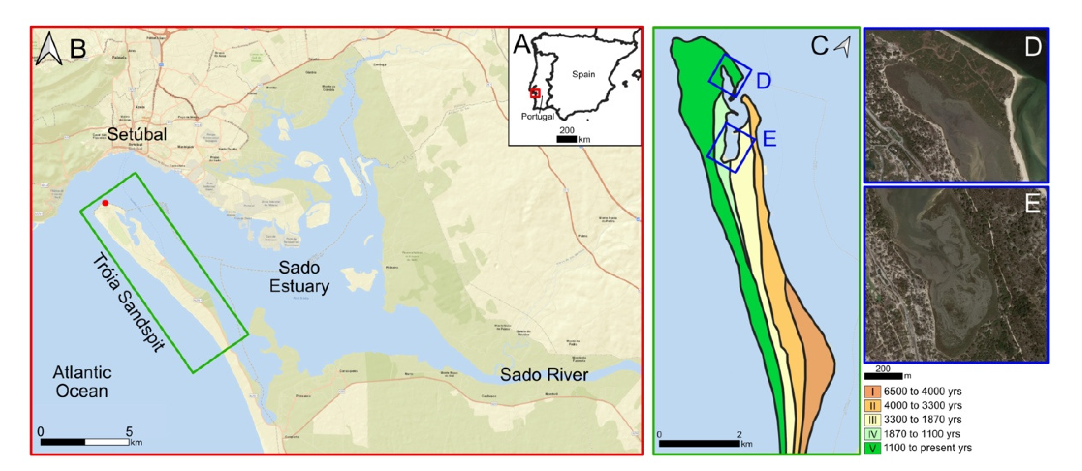
2. Test Areas
3. Models
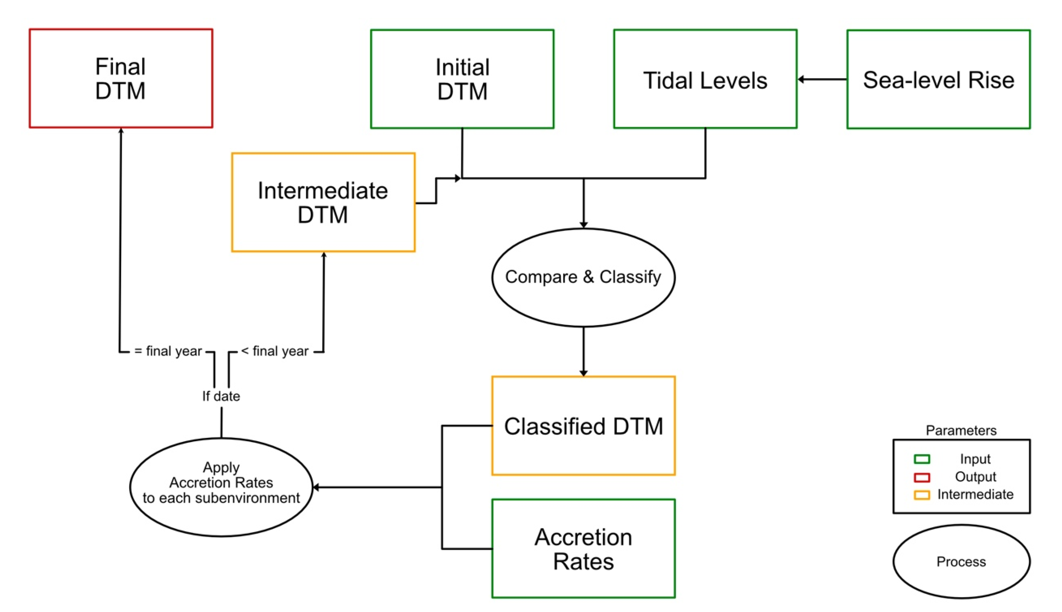
3.1. Simplified Marsh Response Model (SMRM)
3.2. Sea Level Affecting Marsh Model (SLAMM)
4. Parameters
4.1. Local Tidal Levels
4.2. Digital Terrain Model
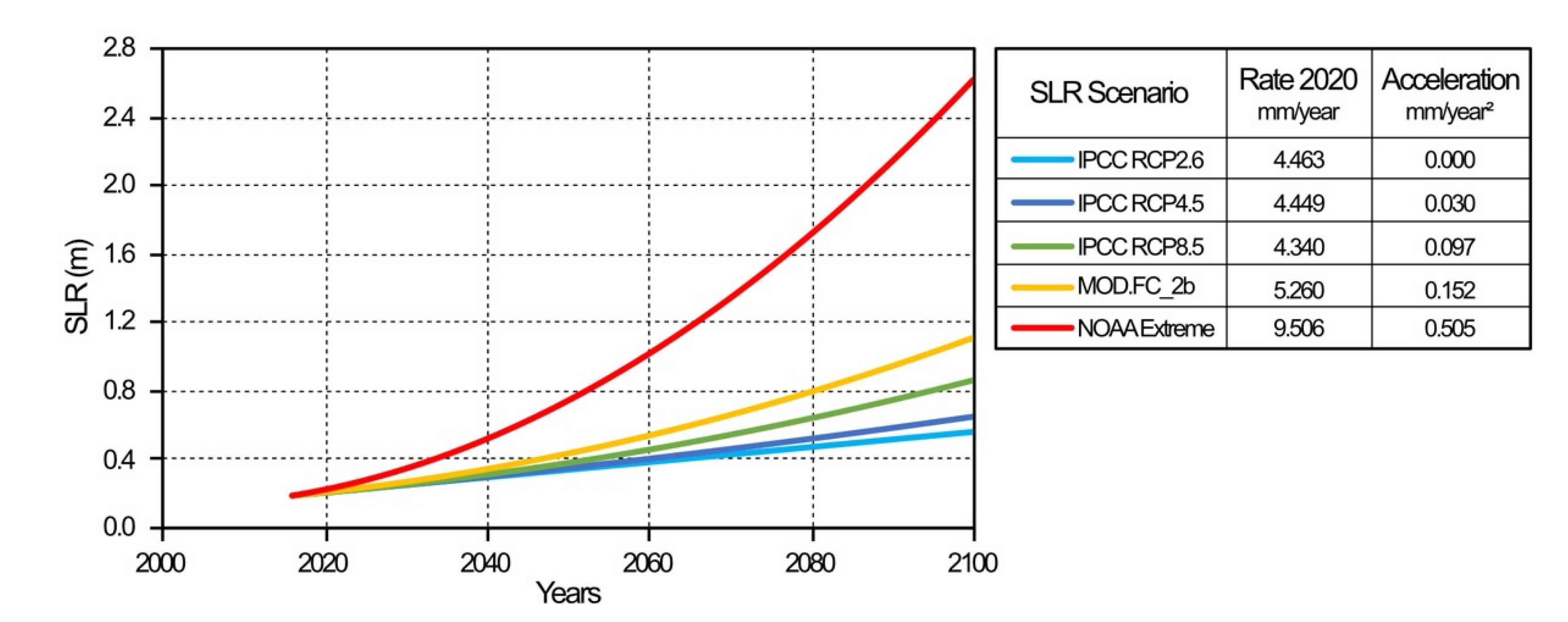
4.3. Sea-Level Rise Scenarios
4.4. Accretion Rates
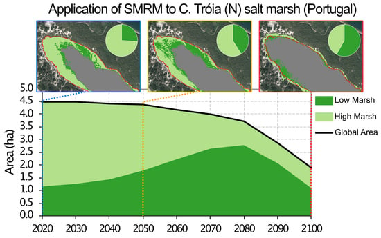
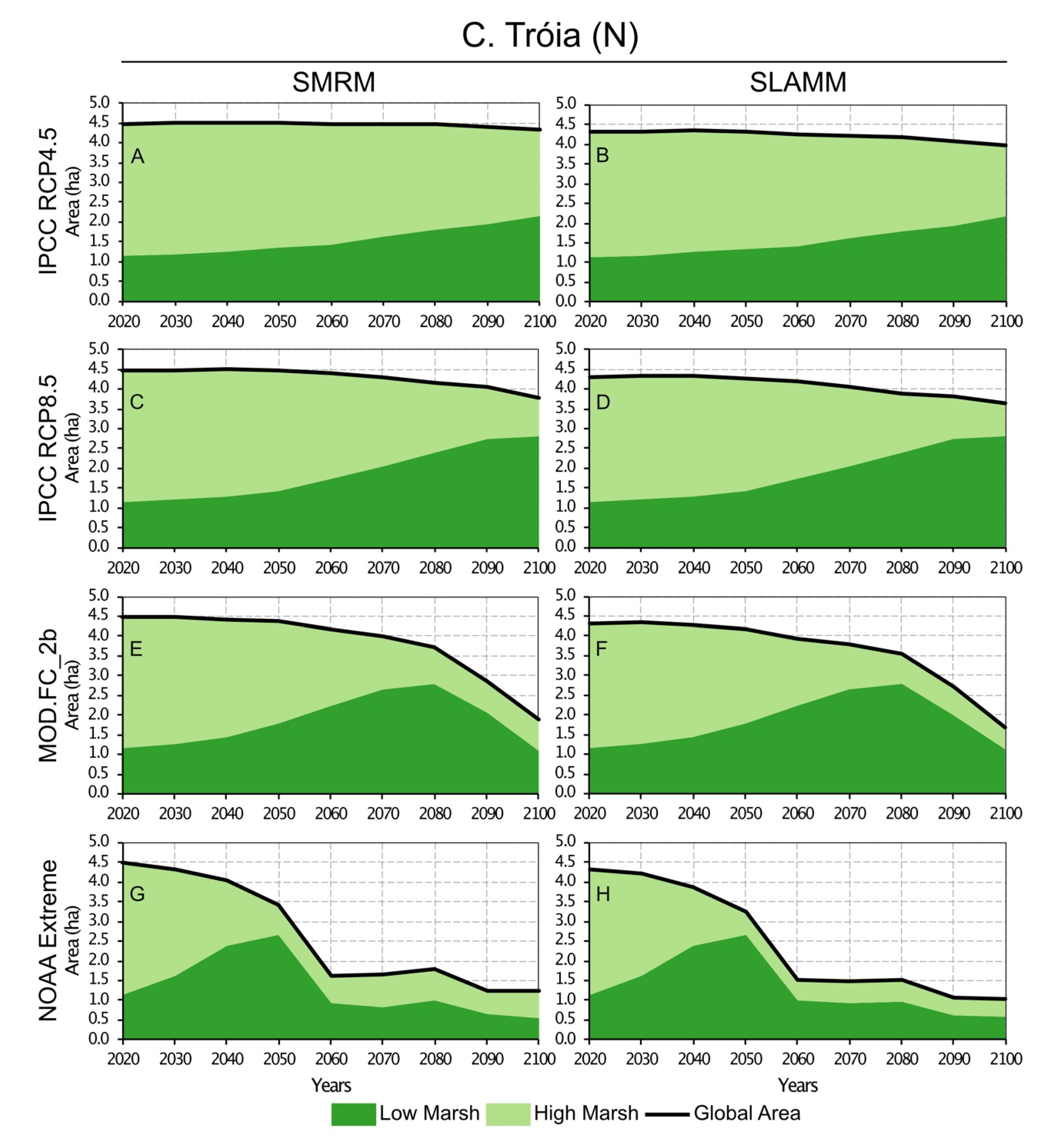
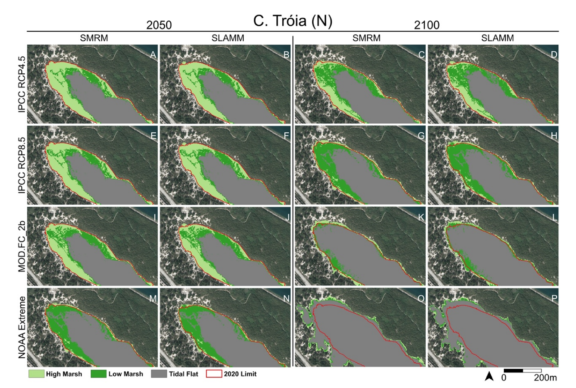
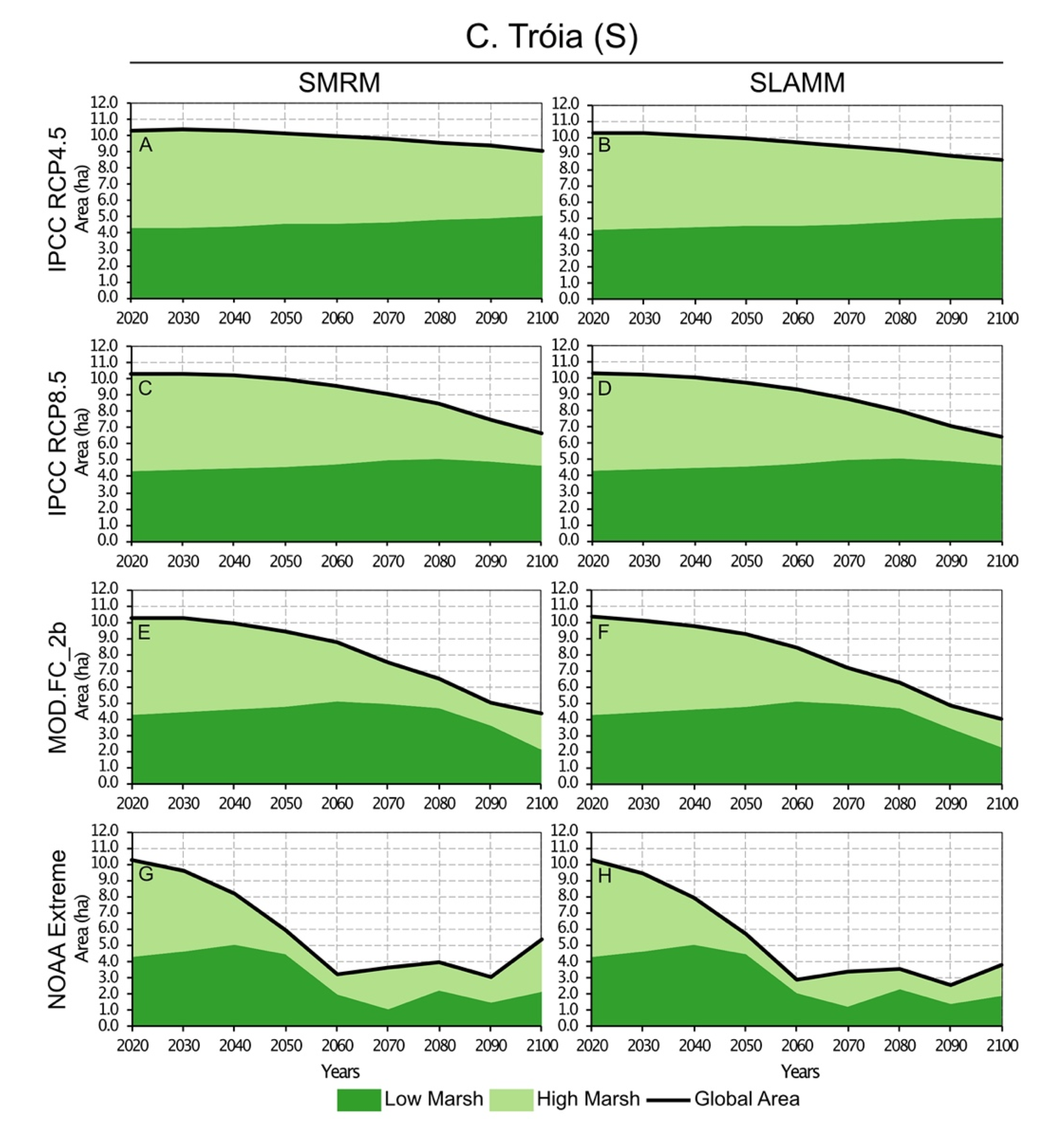
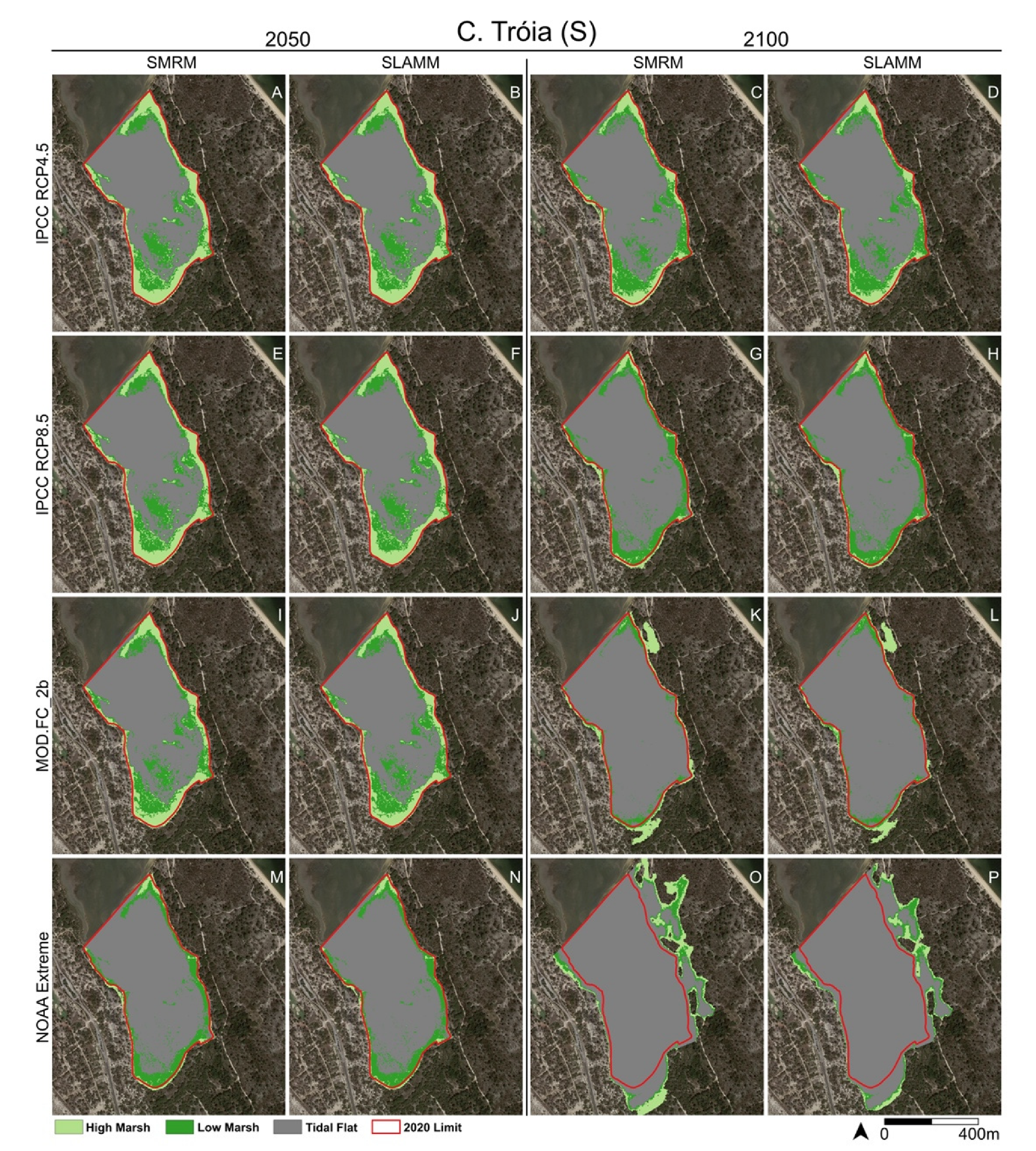
5. Application of SMRM to the Test Areas and Comparison with SLAMM
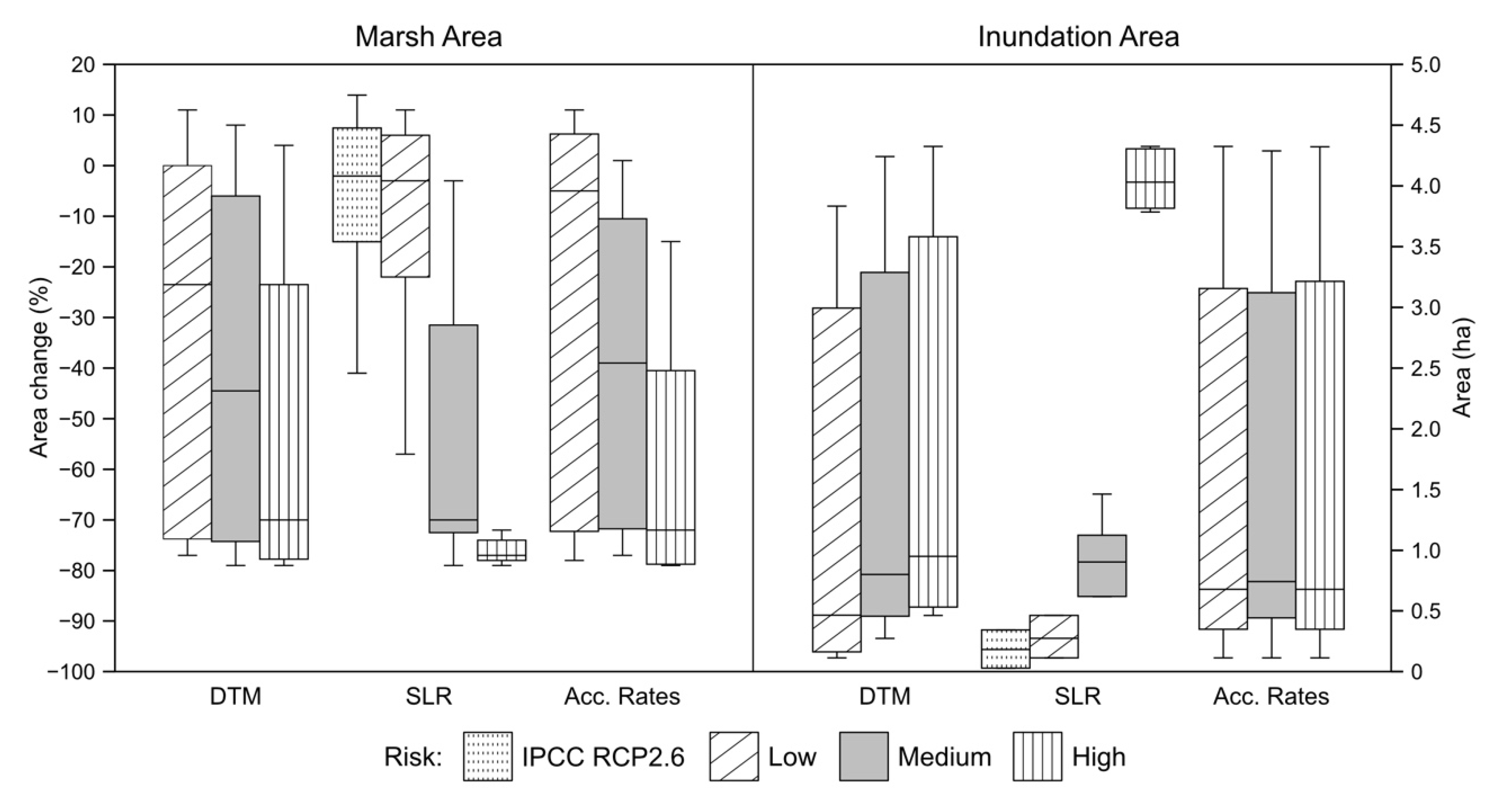
6. Sensitivity Analysis
6.1. Methodology
6.2. Results
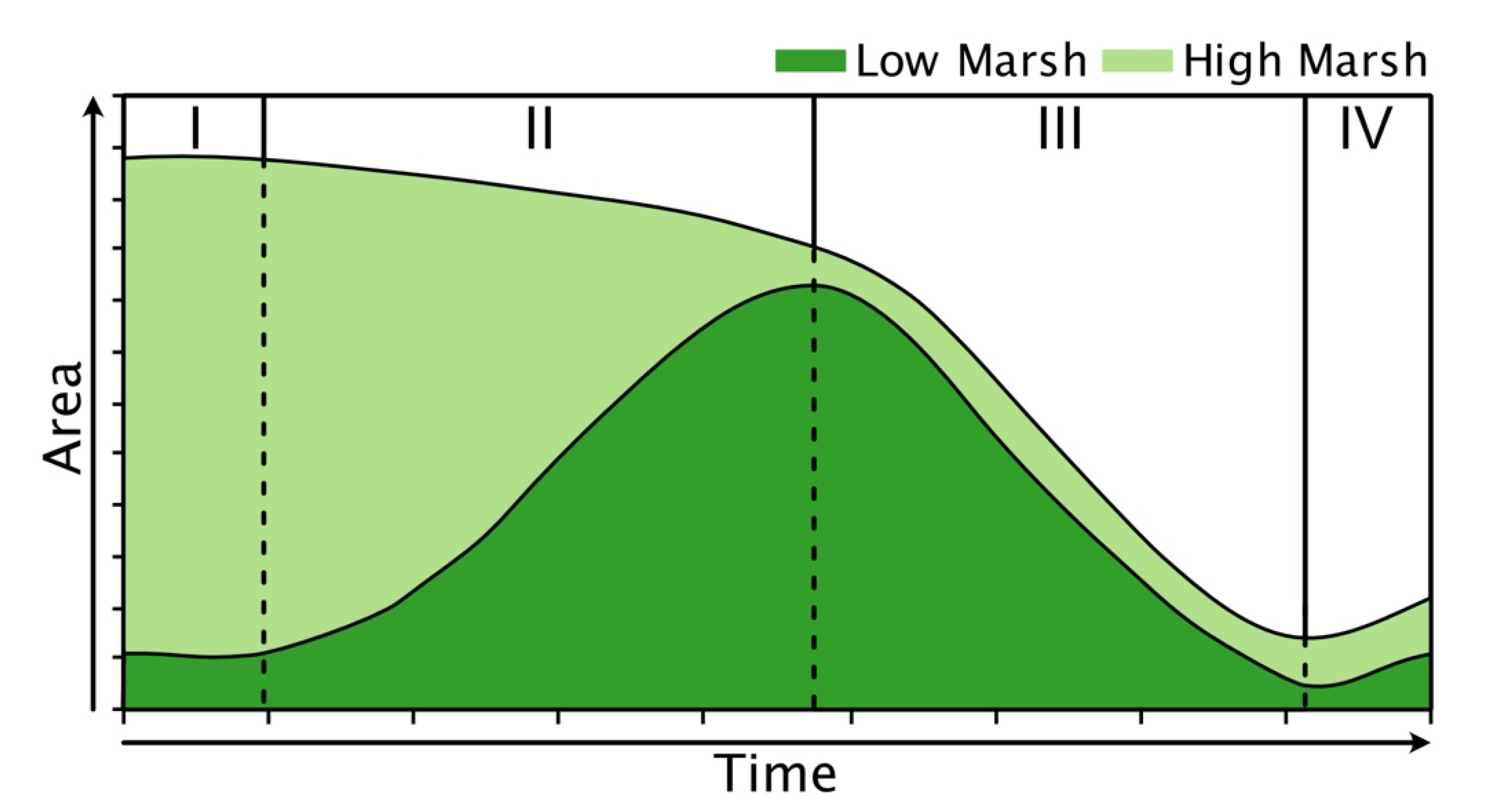
7. Discussion
8. Conclusions
Author Contributions
Funding
Data Availability Statement
Conflicts of Interest
Appendix A. DTM and SLR

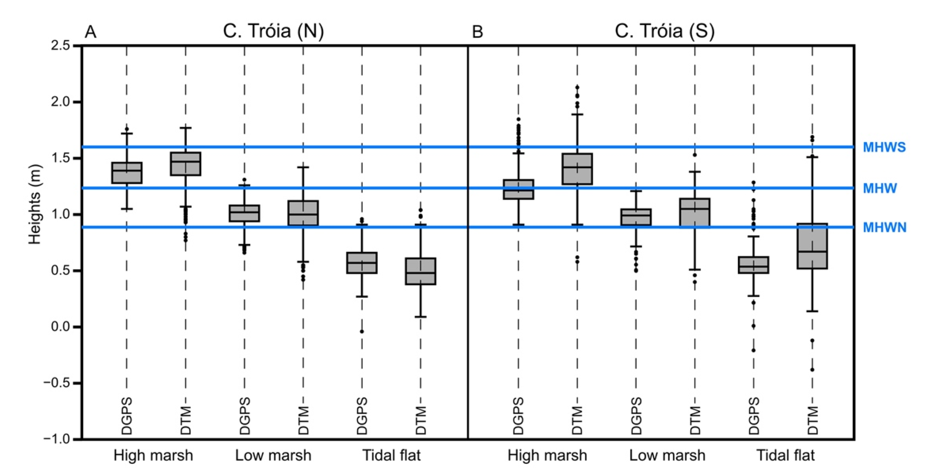
| Parameters | C. Tróia (N) | C. Tróia (S) | ||||||||||
|---|---|---|---|---|---|---|---|---|---|---|---|---|
| High Marsh | Low Marsh | Tidal Flat | High Marsh | Low Marsh | Tidal Flat | |||||||
| DGPS | DTM | DGPS | DTM | DGPS | DTM | DGPS | DTM | DGPS | DTM | DGPS | DTM | |
| Min. (m) | 1.05 | 0.77 | 0.66 | 0.42 | −0.04 | 0.09 | 0.91 | 0.58 | 0.50 | 0.40 | −0.21 | −0.38 |
| Q1 (m) | 1.28 | 1.35 | 0.94 | 0.91 | 0.48 | 0.38 | 1.14 | 1.27 | 0.91 | 0.89 | 0.48 | 0.52 |
| Median (m) | 1.39 | 1.47 | 1.02 | 1.00 | 0.57 | 0.48 | 1.21 | 1.42 | 0.99 | 1.05 | 0.54 | 0.67 |
| Q3 (m) | 1.46 | 1.55 | 1.08 | 1.12 | 0.66 | 0.61 | 1.31 | 1.54 | 1.05 | 1.14 | 0.62 | 0.92 |
| Max. (m) | 1.76 | 1.77 | 1.31 | 1.42 | 0.96 | 1.04 | 1.85 | 2.13 | 1.21 | 1.53 | 1.29 | 1.69 |
| IQR (m) | 0.19 | 0.20 | 0.15 | 0.22 | 0.18 | 0.23 | 0.17 | 0.27 | 0.14 | 0.25 | 0.14 | 0.40 |
| Mean (m) | 1.37 | 1.43 | 1.00 | 1.00 | 0.57 | 0.52 | 1.24 | 1.40 | 0.97 | 1.01 | 0.57 | 0.74 |
| Points | 678 | 928 | 238 | 489 | 191 | 198 | ||||||
| SLR Scenario | Rate 2020 | Acceleration | SLR (cm) | |
|---|---|---|---|---|
| mm/year | mm/year2 | 2050 | 2100 | |
| IPCC RCP2.6 | 4.463 | 0.000 | 33 | 55 |
| IPCC RCP4.5 | 4.449 | 0.030 | 35 | 65 |
| IPCC RCP8.5 | 4.340 | 0.097 | 37 | 86 |
| MOD.FC_2b | 5.260 | 0.152 | 43 | 111 |
| NOAA Extreme | 9.506 | 0.505 | 74 | 261 |
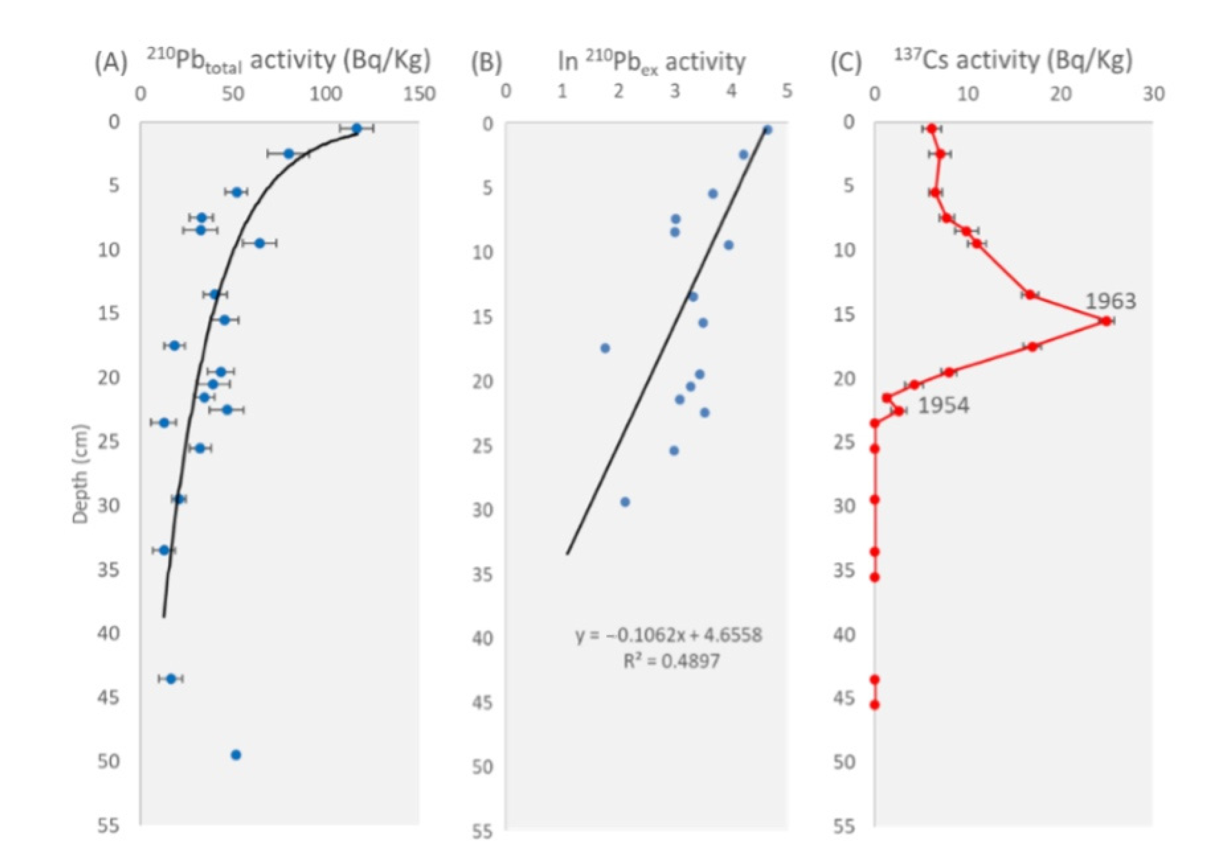
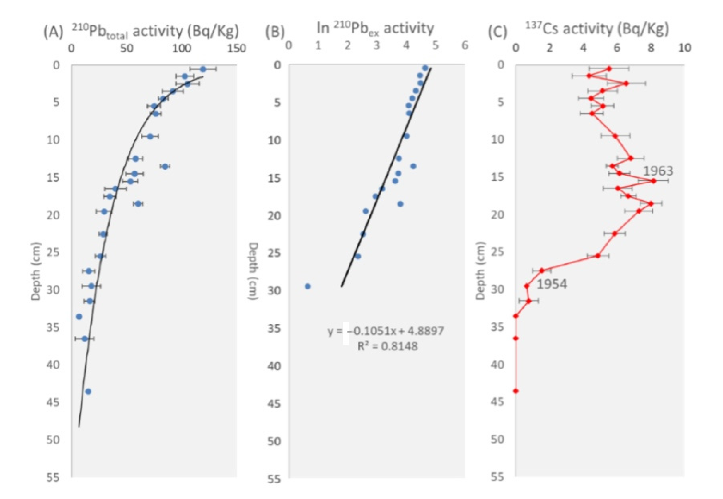
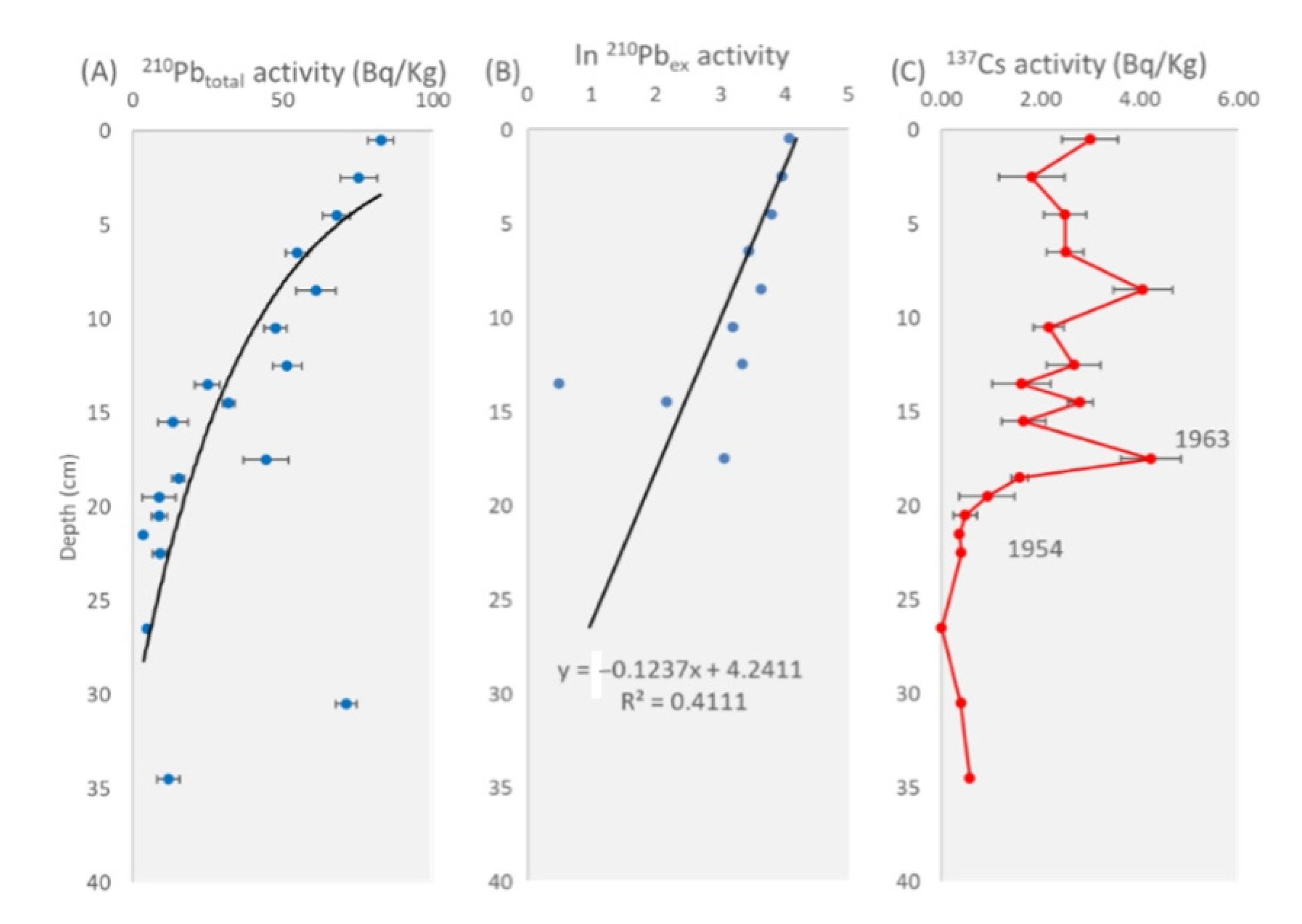
Appendix B. Accretion Rates


| Method | Reference Year | High Marsh | Low Marsh | Tidal Flat |
|---|---|---|---|---|
| 210Pb | - | 2.9 mm/year | 3.0 mm/year | 2.5 mm/year |
| 137Cs | 1963 | 2.9 mm/year | 2.9 mm/year | 3.3 mm/year |
| 1954 | 3.3 mm/year | 4.4 mm/year | 3.6 mm/year |
References
- Vernberg, F.G. Salt-marsh processes: A review. Environ. Toxicol. Chem. 1993, 12, 2167–2195. [Google Scholar] [CrossRef]
- McLeod, E.; Chmura, G.L.; Bouillon, S.; Salm, R.; Bjök, M.; Duarte, C.M.; Lovelock, C.E.; Schlesinger, W.H.; Silliman, B.R. A blueprint for blue carbon: Toward an improved understanding of the role of vegetated coastal habitats in sequestering CO2. Front. Ecol. Environ. 2011, 9, 552–560. [Google Scholar] [CrossRef] [Green Version]
- Boorman, L.A. Salt marshes—Present functioning and future change. Mangroves Salt Marshes 1999, 3, 227–241. [Google Scholar] [CrossRef]
- Davy, A.J. Life on the edge: Saltmarshes ancient and modern. Trans. Norfolk Norwich Nat. Soc. 2009, 42, 1–10. [Google Scholar]
- Valentim, J.M.; Vaz, N.; Silva, H.; Duarte, B.; Caçador, I.; Dias, J.M. Tagus estuary and Ria de Aveiro salt marsh dynamics and the impact of sea level rise. Estuar. Coast. Shelf Sci. 2013, 130, 138–151. [Google Scholar] [CrossRef]
- Fagherazzi, S.; Kirwan, M.L.; Mudd, S.M.; Guntenspergen, G.R.; Temmerman, S.; D’Alpaos, A.; van del Koppel, J.; Rybczyk, J.M.; Reyes, E.; Craft, C.; et al. Numerical models of salt marsh evolution: Ecological, geomorphic, and climatic factors. Rev. Geophys. 2012, 50, RG1002. [Google Scholar] [CrossRef]
- Bouma, T.J.; van Belzen, J.; Balke, T.; van Dalen, J.; Klaassen, P.; Hartog, A.M.; Callaghan, D.P.; Hu, Z.; Stive, M.J.F.; Temmerman, S.; et al. Short-term mudflat dynamics drive long-term cyclic salt marsh dynamics. Limnol. Oceanogr. 2016, 61, 2261–2275. [Google Scholar] [CrossRef]
- Klemas, V. Remote Sensing of Wetlands: Case Studies Comparing Practical Techniques. J. Coast. Res. 2011, 27, 418–427. [Google Scholar] [CrossRef]
- Shanmugam, P. Remote Sensing of the Coastal Ecosystems. J. Geophys. Remote Sens. S 2013, 2, 2169–2249. [Google Scholar] [CrossRef] [Green Version]
- Hardisky, M.A.; Gross, M.F.; Klemas, V. Remote Sensing of Coastal Wetlands: Landsat TM, SPOT, and imaging spectrometers will enhance remote sensing research on wetlands. BioScience 1986, 36, 453–460. [Google Scholar] [CrossRef]
- Goldsmith, S.B.; Eon, R.S.; Lapszynski, C.S.; Badura, G.P.; Osgood, D.T.; Bachmann, C.M.; Tyler, A.C. Assessing Salt Marsh Vulnerability Using High-Resolution Hyperspectral Imagery. Remote Sens. 2020, 12, 2938. [Google Scholar] [CrossRef]
- Doughty, C.L.; Cavanaugh, K.C. Mapping Coastal Wetland Biomass from High Resolution Unmanned Aerial Vehicle (UAV) Imagery. Remote Sens. 2019, 11, 540. [Google Scholar] [CrossRef] [Green Version]
- Oteman, B.; Morris, E.P.; Peralta, G.; Bouma, T.J.; van der Wal, D. Using Remote Sensing to Identify Drivers behind Spatial Patterns in the Bio-physical Properties of a Saltmarsh Pioneer. Remote Sens. 2019, 11, 511. [Google Scholar] [CrossRef] [Green Version]
- Lamb, B.T.; Tzortziou, M.A.; McDonald, K.C. Evaluation of Approaches for Mapping Tidal Wetlands of the Chesapeake and Delaware Bays. Remote Sens. 2019, 11, 2366. [Google Scholar] [CrossRef] [Green Version]
- Pendleton, L.; Donato, D.C.; Murray, B.C.; Crooks, S.; Jenkins, W.A.; Sifleet, S.; Craft, C.; Fourqurean, J.W.; Kauffman, J.B.; Marbà, N.; et al. Estimating global “Blue Carbon” emissions from conversion and degradation of vegetated coastal ecosystems. PLoS ONE 2012, 7, e43542. [Google Scholar] [CrossRef] [Green Version]
- Laffoley, D.; Grimsditch, G.D. The Management of Natural Coastal Carbon Sinks; IUCN Technical Report; IUCN: Gland, Switzerland, 2009. [Google Scholar]
- Luisetti, T.; Jackson, E.L.; Turner, R.K. Valuing the European “coastal blue carbon” storage benefit. Mar. Pollut. Bull. 2013, 71, 101–106. [Google Scholar] [CrossRef]
- Townend, I.; Rossington, K.; Knaapen, M.A.F.; Richardson, S. The dynamics of intertidal mudflats and saltmarshes within estuaries. In Proceedings of the Coastal Engineering Conference, Shanghai, China, 30 June–5 July 2010; Smith, J.M., Lynett, P., Eds.; Coastal Engineering Research Council: Reston, VA, USA, 2010; Volume 32, pp. 1–10. [Google Scholar]
- IPCC. Climate Change 2014: Impacts, Adaptation, and Vulnerability—Part A: Global and Sectoral Aspects. In Contribution of Working Group II to the Fifth Assessment Report of the Intergovernmental Panel on Climate Change; Field, C.B., Barros, V.R., Dokken, D.J., Mach, K.J., Mastrandrea, M.D., Bilir, T.E., Chatterjee, M., Ebi, K.L., Estrada, Y.O., Genova, R.C., et al., Eds.; Cambridge University Press: Cambridge, UK; New York, NY, USA, 2014; p. 1132. [Google Scholar]
- Kirwan, M.L.; Megonigal, J.P. Tidal wetland stability in the face of human impacts and sea-level rise. Nature 2013, 504, 53–60. [Google Scholar] [CrossRef]
- Constanza, R.; Voinov, A. (Eds.) Landscape Simulation Modeling: A Spatially Explicit Dynamic Approach; Springer: Berlin/Heidelberg, Germany, 2004. [Google Scholar] [CrossRef]
- Morris, J.T.; Sundareshwar, P.V.; Nietch, C.T.; Kjerfve, B.; Cahoon, D.R. Responses of coastal wetlands to rising sea level. Ecology 2002, 83, 2869–2877. [Google Scholar] [CrossRef]
- Fagherazzi, S.; Hannion, M.; D’Odorico, P. Geomorphic structure of tidal hydrodynamics in salt marsh creeks. Water Resour. Res. 2008, 44, W02419. [Google Scholar] [CrossRef]
- Raposa, K.B.; Wasson, K.; Smith, E.; Crooks, J.A.; Delgado, P.; Fernald, S.H.; Ferner, M.C.; Helms, A.; Hice, L.A.; Mora, J.W.; et al. Assessing tidal marsh resilience to sea-level rise at broad geographic scales with multi-metric indices. Biol. Conserv. 2016, 204, 263–275. [Google Scholar] [CrossRef] [Green Version]
- Best, S.N.; Van der Wegen, M.; Dijkstra, J.; Willemsen, P.W.J.M.; Borsje, B.W.; Roelvink, D.J.A. Do salt marshes survive sea level rise? Modelling wave action, morphodynamics and vegetation dynamics. Environ. Model. Softw. 2018, 109, 152–166. [Google Scholar] [CrossRef]
- Paola, C.; Leeder, M. Environmental Dynamics: Simplicity versus complexity. Nature 2011, 469, 38–39. [Google Scholar] [CrossRef] [PubMed]
- Murray, A.B. Contrasting the goals, strategies and predictions associated with simplified numerical models and detailed simulations. Predict. Geomorphol. 2003, 135, 151–165. [Google Scholar] [CrossRef]
- French, J.; Payo, A.; Murray, B.; Orford, J.; Eliot, M.; Cowell, P. Appropriate complexity for the prediction of coastal and estuarine geomorphic behaviour at decadal to centennial scales. Geomorphology 2016, 256, 3–16. [Google Scholar] [CrossRef] [Green Version]
- Silva, A.N.; Taborda, R.; Andrade, C.; Ribeiro, M. The future of insular beaches: Insights from a past-to-future sediment budget approach. Sci. Total Environ. 2019, 676, 692–705. [Google Scholar] [CrossRef]
- Silva, M.; Patrício, P.; Mariano, A.; Morais, M.; Valério, M. Obtenção de Dados LiDAR para as Zonas Costeiras de Portugal Continental. Segundas Jorn. Eng. Hidrográfica 2012, 2, 19–22. [Google Scholar]
- Andrade, C.; Pires, H.O.; Taborda, R.; Freitas, M.C. Zonas Costeiras. In Alterações Climáticas em Portugal. Cenários, Impactos e Medidas de Adaptação. Projecto SIAM II, 1st ed.; Santos, F.D., Miranda, P., Eds.; Gradiva: Lisboa, Portugal, 2006; pp. 169–208. [Google Scholar]
- ICNB. Plano Setorial da Rede Natura 2000—1130 Estuários. Instituto da Conservação da Natureza e da Biodiversidade, 2008. Available online: http://www2.icnf.pt/portal/pn/biodiversidade/rn2000/resource/doc/rn-plan-set/hab/hab-1130 (accessed on 1 December 2021).
- EEA. Report under the Article 17 of the habitats Directive—Period 2007–2012. 1130 Estuaries. European Environment Agency, 2013. Available online: https://forum.eionet.europa.eu/habitat-art17report/library/2007-2012-reporting/factsheets/habitats/coastal-habitats/1130-estuaries/download/en/1/1130-estuaries.pdf (accessed on 1 December 2021).
- Guerreiro, V.; Bettencourt, P.; Santos, A. Avaliação de Impactes Ambientais em Sistemas Estuarinos: Revisão de Estudos de Caso nos Estuários do Sado, Mira e Ria Formosa. In Actas do 1.º Simpósio Interdisciplinar de Processos Estuarinos; Universidade do Algarve: Faro, Portugal, 1998. [Google Scholar]
- Bettencourt, A.; Gomes, V.; Dias, A.; Ferreira, G.; Silva, M.; Costa, L. Estuários Portugueses; Direcção dos Serviços de Planeamento, Instituto da Água, Ministério das Cidades, Ordenamento do Território e Ambiente: Lisboa, Portugal, 2003. [Google Scholar]
- Dias, A.A. Estuário do Sado. In Encontro com o Sado; Escola Superior de Educação de Setúbal: Setúbal, Portugal, April 1999; pp. 13–26. [Google Scholar]
- Loureiro, J.M. Monografias Hidrológicas dos Principais Cursos de água de Portugal Continental; Direcção-Geral dos Recursos e Aproveitamentos Hidráulicos: Lisboa, Portugal, 1986. [Google Scholar]
- Moreira, M.E.S.A. Recent Saltmarsh Changes and Sedimentation Rates in the Sado Estuary, Portugal. J. Coast. Res. 1992, 8, 631–640. Available online: https://0-www-jstor-org.brum.beds.ac.uk/stable/4298012 (accessed on 1 December 2021).
- Ambar, I.; Fiúza, A.F.G.; Sousa, F.M.; Lourenço, I.O. General circulation in the lower Sado estuary under drought conditions. In Proceedings of the Actual Problems of Oceanography in Portugal, Lisboa, Portugal, 20–21 November 1980; JNICT/NATO: Lisboa, Portugal, 1982; pp. 97–107. [Google Scholar]
- Neves, R.J.; Ferreira, J.N.R. Modelo Matemático do Estuário do Sado, Extensão à plataforma Costeira Adjacente; Ed Serviço Nacional de Parques e Reservas e Conservação da Natureza: Lisboa, Portugal, 1987. [Google Scholar]
- Costas, S.; Rebêlo, L.; Brito, P.; Burbidge, C.I.; Prudêncio, M.I.; FitzGerald, D. The Joint History of Tróia Peninsula and Sado Ebb-Delta. In Sand and Gravel Spits. Coastal Research Library; Randazzo, G., Jackson, D.W.T., Cooper, J.A.G., Eds.; Springer International Publishing: Basel, Switzerland, 2015; p. 25. [Google Scholar] [CrossRef]
- Davis, R.A.; FitzGerald, D.M. Beaches and Coasts; Blackwell Publishing Company: Hoboken, NJ, USA, 2004. [Google Scholar] [CrossRef]
- MATLAB; 9.4.0.813654 (R2018a); The MathWorks Inc.: Natick, MA, USA, 2018.
- MATLAB; 9.8.0.1380330 (R2020a); The MathWorks Inc.: Natick, MA, USA, 2020.
- ESRI. ArcGIS Pro; Release 2.6.0; Environmental Systems Research Institute: Redlands, CA, USA, 2020. [Google Scholar]
- Inácio, M.; Freitas, M.C.; Cunha, A.G.; Antunes, C.; Leira, M.; Lopes, V.; Andrade, C. SMRM. 2022. Available online: https://figshare.com/articles/software/SMRM/20237409/1 (accessed on 8 July 2022).
- SLAMM. SLAMM 6.7 Technical Documentation; Sea Level Affecting Marshes Model, Version 6.7 Beta; Warren Pinnacle Consulting, Inc.: Waitsfield, VT, USA, 2016. Available online: http://warrenpinnacle.com/prof/SLAMM6/SLAMM_6.7_Technical_Documentation.pdf (accessed on 1 December 2021).
- SLAMM. User’s Manual; SLAMM 6.7 beta; Warren Pinnacle Consulting, Inc.: Waitsfield, VT, USA, 2016. Available online: http://warrenpinnacle.com/prof/SLAMM6/SLAMM_6.7_Users_Manual.pdf (accessed on 1 December 2021).
- Fernandez-Nunez, M.; Burningham, H.; Díaz-Cuevas, P.; Ojeda-Zújar, J. Evaluating the Response of Mediterranean-Atlantic Saltmarshes to Sea-Level Rise. Resources 2019, 8, 50. [Google Scholar] [CrossRef] [Green Version]
- Melet, A.; Meyssignac, B.; Almar, R.; Le Cozannet, G. Under-estimated wave contribution to coastal sea-level rise. Nat. Clim. Chang. 2018, 8, 234–239. [Google Scholar] [CrossRef]
- Antunes, C. Previsão de Marés dos Portos Principais de Portugal. FCUL Webpage, 2007. Available online: http://webpages.fc.ul.pt/~cmantunes/hidrografia/hidro_mares.html (accessed on 1 December 2021).
- Antunes, C. Assessment of sea level rise at West coast of Portugal mainland and its projection for the 21st century. J. Mar. Sci. Eng. 2019, 7, 61. [Google Scholar] [CrossRef] [Green Version]
- Gesch, D.B. Analysis of Lidar Elevation Data for Improved Identification and Delineation of Lands Vulnerable to Sea-Level Rise. J. Coast. Res. 2009, 10053, 49–58. [Google Scholar] [CrossRef]
- Fagherazzi, S. The ephemeral life of a salt marsh. Geology 2013, 41, 943–944. [Google Scholar] [CrossRef] [Green Version]
- Maune, D.F.; Maitra, J.B.; McKay, E.J. Accuracy standards & guidelines. In Digital Elevation Model Technologies and Applications: The DEM Users Manual, 2nd ed.; Maune, D., Ed.; American Society for Photogrammetry and Remote Sensing: Bethesda, MD, USA, 2007; pp. 65–97. [Google Scholar]
- Mendes, V.; Barbosa, S.; Carinhas, D. Vertical land motion in the Iberian Atlantic coast and its implication for sea level change evaluation. J. Appl. Geod. 2020, 14, 361–378. [Google Scholar] [CrossRef]
- Hammond, W.; Blewitt, G.; Kreemer, C.; Nerem, R. GPS Imaging of Global Vertical Land Motion for Studies of Sea Level Rise. J. Geophys. Res. Solid Earth 2021, 126, e2021JB022355. [Google Scholar] [CrossRef]
- IPCC. Climate Change 2013: The Physical Science Basis. In Contribution of Working Group I to the Fifth Assessment Report of the Intergovernmental Panel on Climate Change; Stocker, T.F., Qin, D., Plattner, G.K., Tignor, M., Allen, S.K., Boschung, J., Nauels, A., Xia, Y., Bex, V., Midgley, P.M., Eds.; Cambridge University Press: Cambridge, UK; New York, NY, USA, 2013; p. 1535. [Google Scholar]
- Sweet, V.W.; Kopp, R.E.; Weaver, P.C.; Obeysekera, J.; Horton, M.H.; Thiele, E.R.; Zervas, C. Global and Regional Sea Level Rise Scenarios for the United States; NOAA Technical Report NOS CO-OPS 083; National Oceanic and Atmospheric Admin: Washington, DC, USA, 2017.
- IPCC. Climate Change 2021: The Physical Science Basis. In Contribution of Working Group I to the Sixth Assessment Report of the Intergovernmental Panel on Climate Change; Masson-Delmotte, V., Zhai, P., Pirani, A., Connors, S.L., Péan, C., Berger, S., Caud, N., Chen, Y., Goldfarb, L., Gomis, M.I., et al., Eds.; Cambridge University Press: Cambridge, UK; New York, NY, USA, 2021; in press. [Google Scholar] [CrossRef]
- IPCC. Climate Change 2007: Synthesis Report. In Contribution of Working Groups I, II and III to the Fourth Assessment Report of the Intergovernmental Panel on Climate Change; Core Writing Team, Pachauri, R.K., Reisinger, A., Eds.; IPCC: Geneva, Switzerland, 2007; p. 104. [Google Scholar]
- Fagherazzi, S.; Mariotti, G.; Leonardi, N.; Canestrelli, A.; Nardin, W.; Kearney, W.S. Salt Marsh Dynamics in a Period of Accelerated Sea Level Rise. J. Geophys. Res. Earth Surf. 2020, 125, e2019JF005200. [Google Scholar] [CrossRef]
- Nolte, S.; Koppenaal, E.C.; Esselink, P.; Dijkema, K.S.; Schuerch, M.; De Groot, A.V.; Bakker, J.P.; Temmerman, S. Measuring sedimentation in tidal marshes: A review on methods and their application in biogeomorphological studies. J. Coast. Conserv. 2013, 17, 301–325. [Google Scholar] [CrossRef]
- Freitas, M.C.; Andrade, C.; Cruces, A.; Munhá, J.; Sousa, M.J.; Moreira, S.; Jouanneau, J.M.; Martins, L. Anthropogenic influence in the Sado Estuary (Portugal): A geochemical approach. J. Iber. Geol. 2008, 34, 271–286. [Google Scholar]
- Inácio, M.; Freitas, M.C.; Cunha, A.G.; Antunes, C.; Leira, M.; Lopes, V.; Andrade, C.C. Tróia (N) and (S) SMRM and SLAMM results 2022. Available online: https://figshare.com/articles/dataset/C_Tr_ia_N_and_S_SMRM_and_SLAMM_results/20254425/1 (accessed on 8 July 2022).
- Scardino, G.; Sabatier, F.; Scicchitano, G.; Piscitelli, A.; Milella, M.; Vecchio, A.; Anzidei, M.; Mastronuzzi, G. Sea-Level Rise and Shoreline Changes Along an Open Sandy Coast: Case Study of Gulf of Taranto, Italy. Water 2020, 12, 1414. [Google Scholar] [CrossRef]
- Anzidei, M.; Scicchitano, G.; Scardino, G.; Bignami, C.; Tolomei, C.; Vecchio, A.; Serpelloni, E.; De Santis, V.; Monaco, C.; Milella, M.; et al. Relative Sea-Level Rise Scenario for 2100 along the Coast of South Eastern Sicily (Italy) by InSAR Data, Satellite Images and High-Resolution Topography. Remote Sens. 2021, 13, 1108. [Google Scholar] [CrossRef]
- Gesch, D.B. Consideration of Vertical Uncertainty in Elevation-Based Sea-Level Rise Assessments: Mobile Bay, Alabama Case Study. J. Coast. Res. 2013, 63, 197–210. [Google Scholar] [CrossRef]
- Gesch, D.B. Best Practices for Elevation-Based Assessments of Sea-Level Rise and Coastal Flooding Exposure. Front. Earth Sci. 2018, 6, 230. [Google Scholar] [CrossRef] [Green Version]
- Temmerman, S.; Govers, G.; Meir, P.; Wartel, S. Modelling long-term tidal marsh growth under changing tidal conditions and suspended sediment concentrations, Scheldt Estuary, Belgium. Mar. Geol. 2003, 193, 151–159. [Google Scholar] [CrossRef]
- Laengner, M.L.; Siteur, K.; van der Wal, D. Trends in the Seaward Extent of Saltmarshes across Europe from Long-Term Satellite Data. Remote Sens. 2019, 11, 1653. [Google Scholar] [CrossRef] [Green Version]
- Belliard, J.P.; Di Marco, N.; Carniello, L.; Toffolon, M. Sediment and vegetation spatial dynamics facing sea-level rise in microtidal salt marshes: Insights from an ecogeomorphic model. Adv. Water Resour. 2016, 93, 249–264. [Google Scholar] [CrossRef]
- Kirwan, M.L.; Temmerman, S.; Skeehan, E.E.; Guntenspergen, G.R.; Fagherazzi, S. Overestimation of marsh vulnerability to sea level rise. Nat. Clim. Chang. 2016, 6, 253–260. [Google Scholar] [CrossRef]
- Crosby, S.C.; Sax, D.F.; Palmer, M.E.; Booth, H.S.; Deegan, L.A.; Bertness, M.D.; Leslie, H.M. Salt marsh persistence in threatened by predicted sea-level rise. Estuar. Coast. Shelf Sci. 2016, 181, 93–99. [Google Scholar] [CrossRef] [Green Version]
- Schuerch, M.; Spencer, T.; Temmerman, S.; Kirwan, M.L.; Wolff, C.; Lincke, D.; McOwen, C.J.; Pickering, M.D.; Reef, R.; Vafeidis, A.T.; et al. Future response of global coastal wetlands to sea-level rise. Nature 2018, 561, 231–234. [Google Scholar] [CrossRef]
- Giuliani, S.; Bellucci, L. Salt Marshes: Their Role in Our Society and Threats Posed to Their Existence. In World Seas: An Environmental Evaluation; Sheppard, C., Ed.; Academic Press: Cambridge, MA, USA, 2019; pp. 79–101. [Google Scholar] [CrossRef]
- Macreadie, P.I.; Costa, M.D.P.; Atwood, T.B.; Friess, D.A.; Kelleway, J.J.; Kennedy, H.; Lovelock, C.E.; Serrano, O.; Fuarte, C.M. Blue carbon as a natural climate solution. Nat. Rev. Earth Environ. 2021, 2, 826–839. [Google Scholar] [CrossRef]
- Howard, J.; Sutton-Grier, A.; Herr, D.; Kleypas, J.; Landis, E.; Mcleod, E.; Pidgeon, E.; Simpson, S. Clarifying the role of coastal and marine systems in climate mitigation. Front. Ecol. Environ. 2017, 15, 42–50. [Google Scholar] [CrossRef]
- Duarte, B.; Carreiras, J.; Caçador, I. Climate Change Impacts on Salt Marsh Blue Carbon, Nitrogen and Phosphorous Stocks and Ecosystem Services. Appl. Sci. 2021, 11, 1969. [Google Scholar] [CrossRef]
- Farris, A.S.; Defne, Z.; Ganju, N.K. Identifying Salt Marsh Shorelines from Remotely Sensed Elevation Data and Imagery. Remote Sens. 2019, 11, 1795. [Google Scholar] [CrossRef] [Green Version]
- Giorgi, F.; Lionello, P. Climate change projections for the Mediterranean region. Glob. Planet. Chang. 2007, 63, 90–104. [Google Scholar] [CrossRef]
- Lionello, P.; Özsoy, E.; Planton, S.; Zanchetta, G. Climate Variability and Change in the Mediterranean Region. Glob. Planet. Chang. 2017, 151, 1–3. [Google Scholar] [CrossRef]
- Appleby, P.G. Chronostratigraphic techniques in recent sediments. In Tracking Environmental Change Using Lake Sediments Volume 1: Basin Analysis, Coring, and Chronological Techniques; Last, W.M., Smol, J.P., Eds.; Kluwer Academic: Dordrecht, The Netherlands, 2001; pp. 171–203. [Google Scholar]
- Sanchez-Cabeza, J.A.; Ruiz-Fernández, A.C. 210Pb sediment radiochronology: An integrated formulation and classification of dating models. Geochim. Cosmochim. 2012, 82, 183–200. [Google Scholar] [CrossRef]


| Situation | Possible Result |
|---|---|
| SLR rates < Acc. rates | Expansion |
| SLR rates ≈ Acc. rates | Stability |
| SLR rates > Acc. rates | Inundation |
| SMRM | |||
|---|---|---|---|
| MSL | MHWN | MHW | MHWS |
| 0.19 m | 0.90 m | 1.26 m | 1.61 m |
| SLAMM | |||
| MSL | 90 days | 60 days | 30 days |
| 0.19 m | 1.32 m | 1.47 m | 1.62 m |
| SLAMM site-specific parameters | |||
| Great Diurnal Tidal Range | Salt Elevation | ||
| 2.14 m | 1.62 m | ||
| C. Tróia (N) | |||||
|---|---|---|---|---|---|
| Global | Dune | High marsh | Low marsh | Tidal flat | |
| RMSE | 17 cm | 29 cm | 13 cm | 18 cm | 14 cm |
| L.E. | 33 cm | 57 cm | 25 cm | 36 cm | 27 cm |
| C. Tróia (S) | |||||
| Global | Dune | High marsh | Low marsh | Tidal flat | |
| RMSE | 22 cm | 39 cm | 21 cm | 15 cm | 31 cm |
| L.E. | 43 cm | 76 cm | 41 cm | 29 cm | 60 cm |
| Scenario | SMRM | SLAMM | ||||||||||||
|---|---|---|---|---|---|---|---|---|---|---|---|---|---|---|
| 2020 | 2050 | 2100 | 2020 | 2050 | 2100 | |||||||||
| Area (ha) | HM/LM | Area (ha) | HM/LM | Area (ha) | HM/LM | Area (ha) | HM/LM | Area (ha) | HM/LM | Area (ha) | HM/LM | |||
| C. Tróia (N) | IPCC | RCP4.5 | 4.48 | 2.9 | 4.49 | 2.3 | 4.33 | 1.0 | 4.31 | 2.8 | 4.30 | 2.2 | 3.99 | 0.8 |
| RCP8.5 | 4.45 | 2.1 | 3.79 | 0.4 | 4.27 | 2.0 | 3.63 | 0.3 | ||||||
| MOD.FC_2b | 4.36 | 1.4 | 1.89 | 0.7 | 4.17 | 1.3 | 1.67 | 0.5 | ||||||
| NOAA Extreme | 3.42 | 0.3 | 1.25 | 1.2 | 3.25 | 0.2 | 1.03 | 0.8 | ||||||
| C. Tróia (S) | IPCC | RCP4.5 | 10.29 | 1.4 | 10.12 | 1.2 | 9.10 | 0.8 | 10.31 | 1.4 | 9.93 | 1.2 | 8.60 | 0.7 |
| RCP8.5 | 9.95 | 1.2 | 6.65 | 0.4 | 9.74 | 1.1 | 6.37 | 0.4 | ||||||
| MOD.FC_2b | 9.44 | 1.0 | 4.39 | 1.1 | 9.22 | 0.9 | 4.01 | 0.8 | ||||||
| NOAA Extreme | 5.98 | 0.3 | 5.40 | 1.5 | 5.71 | 0.3 | 3.81 | 1.0 | ||||||
| Risk | DTM | SLR | Acc. Rates |
|---|---|---|---|
| IPCC RCP2.6 | |||
| Low | SLR − RMSE | IPCC RCP4.5 | 5.46/5.84 mm/year (tidal flat/marsh) |
| Medium | - | MOD.FC_2b | 2.73/2.92 mm/year (tidal flat/marsh) |
| High | SLR + RMSE | NOAA Extreme | 0 mm/year |
Publisher’s Note: MDPI stays neutral with regard to jurisdictional claims in published maps and institutional affiliations. |
© 2022 by the authors. Licensee MDPI, Basel, Switzerland. This article is an open access article distributed under the terms and conditions of the Creative Commons Attribution (CC BY) license (https://creativecommons.org/licenses/by/4.0/).
Share and Cite
Inácio, M.; Freitas, M.C.; Cunha, A.G.; Antunes, C.; Leira, M.; Lopes, V.; Andrade, C.; Silva, T.A. Simplified Marsh Response Model (SMRM): A Methodological Approach to Quantify the Evolution of Salt Marshes in a Sea-Level Rise Context. Remote Sens. 2022, 14, 3400. https://0-doi-org.brum.beds.ac.uk/10.3390/rs14143400
Inácio M, Freitas MC, Cunha AG, Antunes C, Leira M, Lopes V, Andrade C, Silva TA. Simplified Marsh Response Model (SMRM): A Methodological Approach to Quantify the Evolution of Salt Marshes in a Sea-Level Rise Context. Remote Sensing. 2022; 14(14):3400. https://0-doi-org.brum.beds.ac.uk/10.3390/rs14143400
Chicago/Turabian StyleInácio, Miguel, M. Conceição Freitas, Ana Graça Cunha, Carlos Antunes, Manel Leira, Vera Lopes, César Andrade, and Tiago Adrião Silva. 2022. "Simplified Marsh Response Model (SMRM): A Methodological Approach to Quantify the Evolution of Salt Marshes in a Sea-Level Rise Context" Remote Sensing 14, no. 14: 3400. https://0-doi-org.brum.beds.ac.uk/10.3390/rs14143400