Article

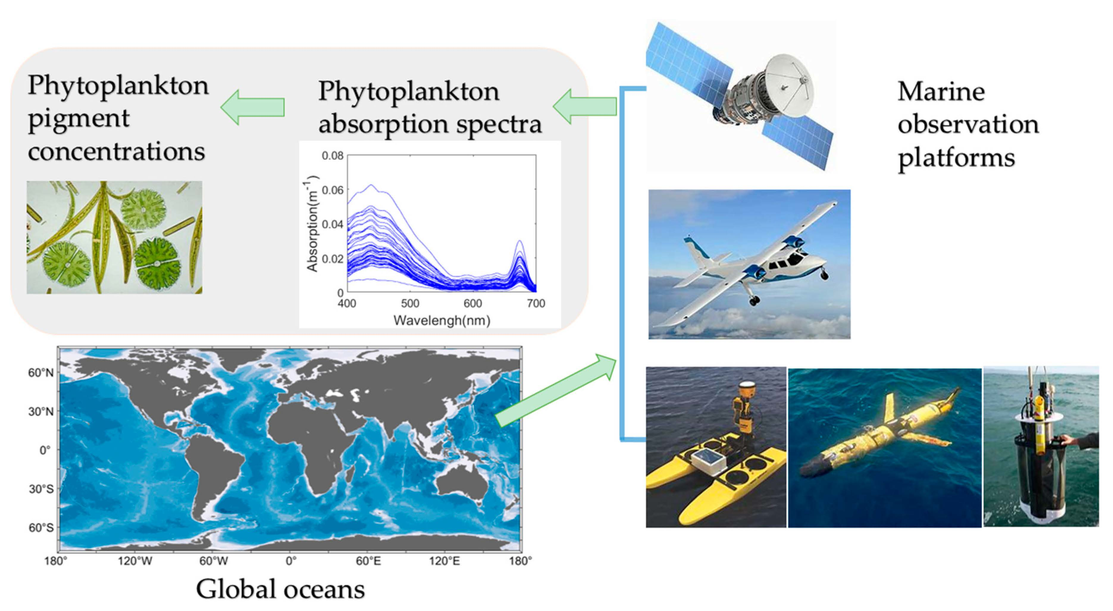
Retrieving Pigment Concentrations Based on Hyperspectral Measurements of the Phytoplankton Absorption Coefficient in Global Oceans

1
Department of Marine Technology, College of Information Science and Engineering, Ocean University of China, Qingdao 266100, China
2
Laboratory for Regional Oceanography and Numerical Modeling, Pilot National Laboratory for Marine Science and Technology (Qingdao), Qingdao 266237, China
*
Author to whom correspondence should be addressed.
Remote Sens. 2022, 14(15), 3516; https://0-doi-org.brum.beds.ac.uk/10.3390/rs14153516
Submission received: 17 June 2022 / Revised: 16 July 2022 / Accepted: 18 July 2022 / Published: 22 July 2022
(This article belongs to the Special Issue Bio-Optical Oceanic Remote Sensing)

Abstract

:
Phytoplankton communities, which can be easily observed by optical sensors deployed on various types of platforms over diverse temporal and spatial scales, are crucial to marine ecosystems and biogeochemical cycles, and accurate pigment concentrations make it possible to effectively derive information from them. To date, there is no practical approach, however, to retrieving concentrations of detailed pigments from phytoplankton absorption coefficients ( a ph ) with acceptable accuracy and robustness in global oceans. In this study, a novel method, which is a stepwise regression method improved by early stopping (the ES-SR method) based on the derivative of hyperspectral a ph , was proposed to retrieve pigment concentrations. This method was developed from an extensive global dataset collected from layers at different depths and contains phytoplankton pigment concentrations and a ph . In the case of the logarithm, strong correlations were found between phytoplankton pigment concentrations and the absolute values of the second derivative ( a ph )/the fourth derivative ( a ph 4 ) of a ph . According to these correlations, the ES-SR method is effective in obtaining the characteristic wavelengths of phytoplankton pigments for pigment concentration inversion. Compared with the Gaussian decomposition method and principal component regression method, which are based on the derivatives, the ES-SR method implemented on a ph is the optimum approach with the greatest accuracy for each phytoplankton pigment. More than half of the determination coefficient values ( R 2 log ) for all pigments, which were retrieved by performing the ES-SR method on a ph , exceeded 0.7. The values retrieved for all pigments fit well to the one-to-one line with acceptable root mean square error ( RMSE log : 0.146–0.508) and median absolute percentage error ( MPE log : 8.2–28.5%) values. Furthermore, the poor correlations between the deviations from the values retrieved by the ES-SR method and impact factors related to pigment composition and cell size class show that this method has advantageous robustness. Therefore, the ES-SR method has the potential to effectively monitor phytoplankton community information from hyperspectral optical data in global oceans.

Graphical Abstract

1. Introduction

Phytoplankton, as the primary production, is fundamental in the ocean, and its communities, characterized by a high degree of taxonomic diversity, are closely related to marine ecosystems and biogeochemical function, especially for the health of marine environments and global carbon cycling, which have been increasingly studied [1,2,3,4,5,6]. Hence, it is of substantial interest to efficiently and effectively derive information on phytoplankton biomass and community composition at the regional and, even, global scales.
Many in situ approaches have been developed to measure phytoplankton community structure, including microscopic taxonomy and cell counting, flow cytometric sorting and enumeration, DNA meta-barcoding, and pigment chemotaxonomy via high-performance liquid chromatography, with respective advantages at identifying phytoplankton, but the field sampling required by these methods cannot meet the ocean observation requirements with border scope and higher density at spatial and temporal scales [7,8,9]. Due to the widespread deployment of optical sensors on different monitoring platforms, e.g., fixed or moving platforms (such as profiling floats, autonomous underwater gliders, and unmanned surface vehicles), aircraft platforms and satellites, it is easy to obtain optical data at high temporal and spatial resolutions [10,11,12]. In particular, the development of satellites offers the possibility of rapid and repeated observations of global marine phytoplankton. In addition, with continuous advances in hyperspectral technology to provide more useful spectral characteristics of unique phytoplankton communities [13,14,15], it is becoming more important to determine how to effectively extract phytoplankton community information from hyperspectral optical data.
Many studies have indicated that phytoplankton absorption coefficients ( a ph ), which utilize optical approaches, can be retrieved from hyperspectral remote sensing reflectance and particulate absorption coefficients, which are generally acquired through optical observation platforms [10,12,16,17,18]. The features of a ph are sensitive to phytoplankton community information, and a ph values are increasingly applied to infer phytoplankton pigment concentrations, phytoplankton cell size and taxonomic information (e.g., harmful species) [9,19,20,21,22,23,24,25]. Moreover, phytoplankton cell size and community composition can be quantified using pigment chemotaxonomy methods, such as CHEMTAX [26,27,28] and diagnostic pigment analyses, in case there are reliable phytoplankton pigment concentrations [29,30,31,32]. Therefore, a ph is a potential tool for studying phytoplankton communities with high efficiency and feasibility. It is crucial to obtain a practical approach to retrieve concentrations of various detailed pigments from a ph with acceptable accuracy and robustness in global oceans.
There are several types of methods for retrieving pigment concentrations from a ph using the distinctive absorption characteristics of different pigments, such as principal component regression based on derivatives [9], the Gaussian decomposition method [10,12,33,34] and the matrix inversion method [12,23,35]. These methods are only tested and found to be suitable for surface or regional water samples, with reasonable results obtained for partial pigments. Moisan et al. used the matrix inversion method to obtain pigment concentrations from a large global ocean dataset, but the results can only be applied well in regional seas [23]. Chase et al. used the Gaussian decomposition method to accurately obtain the concentrations of pigment groups, e.g., photoprotective (PPC) and photosynthetic (PSC) carotenoids, but detailed pigments, e.g., fucoxanthin (Fuco) and alloxanthin (Allo), can hardly be distinguished by this method [10]. Catlett and Siegel developed an inversion method that combines the principal component regression method with the first and second derivative spectra to retrieve pigments, and the method is well suited for some detailed pigments, such as Fuco and peridinin (Perid) [9]. Due to the limitation of inversion methods or sampling ranges in previous studies until now, there has been no practical approach for retrieving the concentrations of most detailed pigments from a ph with acceptable accuracy and robustness in global oceans.
Numerous studies have shown that the transformation of derivatives, especially the second and fourth derivatives of hyperspectral optical data, can effectively enhance the absorption characteristics of phytoplankton pigments or species and can help reduce the pigment packaging effect, which depends mainly on phytoplankton cell size [8,9,19,36,37,38,39,40,41,42]. In addition, phytoplankton cell size and pigment composition are the main factors causing obvious discrepancies in specific absorption coefficients [43,44,45,46], and their influence on the accuracy of inversion methods is to be studied. Stepwise regression, as a popular high-efficiency data-mining tool, can obtain an optimum set of explanatory variables for modelling [47,48,49], which has great potential for pigment concentration inversion. Given the issues mentioned above, a scheme based on the second or fourth derivative of a ph and stepwise regression to estimate pigment concentrations was proposed, and the idea of evaluating inversion methods using impact factors related to phytoplankton size class and pigment composition was developed.
To establish an inversion method that can be applied not only to the sea surface layer, which can be easily derived by satellites, but also to deeper layers, which can be observed by profiling optical instruments in any waters of the global oceans, it is necessary to gather a dataset from diverse environments and different sampling depths. Here, an extensive dataset from global oceans at different depths was collected and analysed to elucidate the characteristics among phytoplankton pigment concentrations and matched a ph values. The data analysis was used to guide the establishment of the global inversion method, a stepwise regression method improved by early stopping (the ES-SR method), to retrieve pigment concentrations from the derivative of a ph . The performance of the ES-SR method was then assessed by comparison and analyses combining the inversion results obtained with various methods and the impact factors.
The paper is organized as follows. In Section 2, the global datasets and their processing procedures are described. The characteristics of the research data are analysed in Section 3, and the novel method is introduced in detail. The performance of this method is assessed in Section 4. The conclusions are organized and given in Section 5.

2. Study Area and Data

2.1. Study Area

A total of 4604 match-ups, which consisted of hyperspectral a ph and phytoplankton pigment concentrations, were obtained from SeaWiFS Bio-optical Archive and Storage System (SeaBASS) [50]. These match-ups were collected from oligotrophic oceans to turbid coasts between August 1996 and December 2017 and were quality controlled [51]. Figure 1 and Table 1 show the locations of the sampling stations and general data information, respectively. The distribution of seawater samples used in this study can roughly reflect the overall global ocean water information.

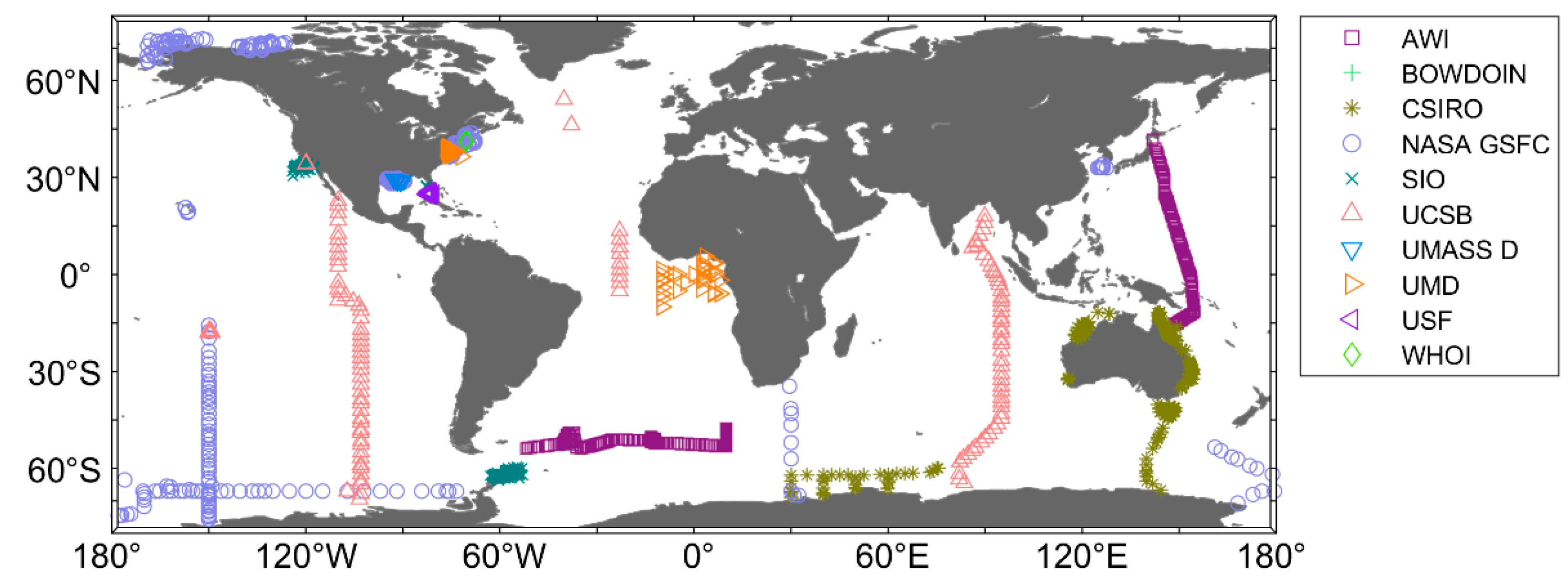
2.2. Data and Preprocessing

2.2.1. Phytoplankton Pigments

Discrete seawater samples were collected, filtered, flash-frozen and stored initially in liquid nitrogen until analysis in the laboratory. Then, phytoplankton pigments were extracted and analysed with a high-performance liquid chromatography (HPLC) method (pigment concentration units of mg m−3). Each of the pigments, which are considered critical in identifying the types of most phytoplankton communities in the ocean, are listed in Appendix A, along with their respective abbreviations and known taxonomic distributions [9,28,29,32]. The inversion objectives of this paper are five pigment groups (total chlorophyll (a, b and c), PSC and PPC) and eighteen detailed pigments (e.g., Fuco and Allo) in Table A1. Because of the large number of sources of this dataset, it is not practical to detail every cruise and the various laboratory processing methods involved in obtaining phytoplankton pigment concentrations. Specific criteria can be found on the SeaBASS website [52].

2.2.2. Phytoplankton Absorption Coefficient

Seawater samples for the determination of a ph were gathered by utilizing similar methods used for phytoplankton pigment samples. Using the quantitative filter technique (QFT), the particulate absorption coefficient ( a p ) of the filters was measured first. Then, the filters were extracted to remove phytoplankton pigments and other organic-soluble material. Finally, the detrital absorption coefficient ( a d ) of the extracted filters was measured and subtracted from a p to yield a ph [15,53]. To facilitate the establishment and parameter analysis of inversion methods, all a ph spectra (in absorption units of m−1) were resampled at 1 nm resolution using the cubic spline interpolation method. The spectral range of a ph was selected in the 400–700 nm range, which contains most information on phytoplankton pigment absorption.
To provide a helpful means of assessing pigment concentrations, the a ph spectra were processed by the Savitzky–Golay derivative transformation with a 31 nm window, which is close to the full width at half the maximum of pigment absorption peaks. The processed a ph can overall optimize the linear relationships between phytoplankton pigment concentrations and the corresponding first, second and fourth derivatives of a ph . In addition, to eliminate the measurement noise in a ph spectra, a Savitzky–Golay smoothing filter with an 11 nm window, which can remove noise and retain detailed a ph information, was applied to each a ph prior to derivation.

3. ES-SR Method

The phytoplankton absorption spectrum is the sum of all pigment absorption spectra. The absorption of light by various pigments in phytoplankton has wavelength selectivity, and each pigment has a specific absorption spectrum (as shown in Figure 2) [30,54]. Due to the extensive presence of chlorophyll a, the absorption peaks at 440 nm in the blue band and 675 nm in the red band are always present. In addition, the peaks in the blue band are broadened and enhanced due to the presence of accessory pigments, and the other corresponding bands also showed changes. Therefore, changes in the shape of the phytoplankton absorption spectrum can reflect changes in the pigment composition. However, as shown in Figure 2, the absorption spectra of some pigments are very similar (generally for the same type of pigments), such as Fuco and HexFuco, making the inversion of these pigments difficult. The shape of phytoplankton absorption spectra is influenced not only by pigment composition but also by morphological features such as phytoplankton cell size class [44,45,46], the so-called “pigment packaging effect”, which is one of the most challenging problems in retrieving pigment concentrations based on absorption spectra. To cope with these difficulties, this paper proposes a novel inversion method based on data characterization to improve the accuracy of pigment concentration inversion. The following will describe how the method was constructed.

3.1. Variable Form for Inversion

The phytoplankton pigment concentrations and absorption spectra of the global data were characterized, mainly using the formal normality test [55,56] and correlation coefficients, in Appendix B to guide the establishment of the inversion method, as well as to provide a basis for the interpretation of the inversion results. Global phytoplankton pigment concentrations depart substantially from normality, and the pigment concentrations of different samples may vary by multiple orders of magnitude, while the log-transformed pigment concentrations conform well to the normal distribution. There are strong correlations between many phytoplankton pigment concentrations, which can affect the accuracy of inversion models. Derivative transformation of a ph can mitigate the multicollinearity problem of pigment concentration inversion.
Based on the data analysis above, the dependent variable should be the log-transformed pigment concentration, which has poor correlations with the values of a ph and a ph 4 in global oceans. Hence, the novel explanatory variable needs to be explored for modelling. After testing various mathematical transformations of derivative spectra, strong correlations (Pearson’s correlation coefficients, R) were finally found between the logarithm of pigment concentrations and log-transformed absolute values of a ph and a ph 4 in some wavelength intervals (Figure 3).
The correlation spectra of various phytoplankton pigments are shown in Figure 3. The correlation spectra of pigments have similar shapes except for those of DVChla, DVChlb, ButFuco, HexFuco, Zea and Pras. In addition, the correlation spectra of DVChla and DVChlb are similar in shape, as are those of ButFuco and HexFuco. Coincidentally, the concentrations of DVChla, DVChlb, ButFuco, HexFuco, Zea and Pras showed low correlations with the concentrations of the remaining pigments, and there was a strong correlation between the concentrations of DVChla and DVChlb (Rs = 0.75), as did those of ButFuco and HexFuco (Rs = 0.65), as shown in Figure A1. Therefore, the strong correlations between pigment concentrations may lead to a deceptively strong correlation between the target pigment concentration and the absorption spectral features of some other interfering pigments, and similar conclusions can be drawn from the results of Catlett & Siegel [9]. For example, carotenoids have no obvious absorption features at 670–680 nm, and TChla has a strong absorption peak in this band, but a strong correlation still appears between the concentrations of many carotenoids (e.g., Fuco, etc.) and the absorption characteristics at 670–680 nm (Figure 3), which may be due to the strong correlation between the concentrations of carotenoids and TChla. These strong but physically meaningless correlations are rarely identified by statistical methods, so prior knowledge of the relevant pigment absorption features should be used to guide the establishment of pigment concentration inversion methods.

3.2. Ideas and Rationale for the Establishment of the ES-SR Method

As a high-efficiency data-mining tool, stepwise regression is widely used to select a subset of explanatory variables from a dataset based on statistical significance for modelling [47,48,49]. This method can effectively circumvent the computational burden of trying all possible combinations of explanatory variables and gives a reasonable approximation to the results of a full data-mining search [49]. The number of parameters in the stepwise regression model is expected to be significantly less than that in the full model, and the variance of estimated parameters can also be effectively reduced. Therefore, the stepwise regression method has great potential for the inversion of phytoplankton pigment concentrations.
Nonetheless, to retrieve phytoplankton pigment concentrations from a subset of explanatory variables obtained from hyperspectral a ph by stepwise regression, some problems should be solved in advance. The first problem is that explanatory variables were chosen exclusively based on statistical criteria without considering whether they were actually significant. In other words, some real explanatory variables have causal effects on the dependent variable, which may not be statistically significant, while nuisance variables may be coincidentally significant [49]. As a result, some real explanatory variables may be omitted, and some nuisance variables may be wrongly chosen for the inversion model. This model may fit the in-sample data well but may fit the out-of-sample data poorly. The second problem is that the larger the number of potential explanatory variables is, the less effective is the stepwise regression method. Paradoxically, the more information there is, the more difficult it is to extract its meaning [57]. In particular, big data, which have too many potential explanatory variables, exacerbate the failings of stepwise regression. Coincidentally, there are hundreds of candidates from hyperspectral a ph that could be used to choose the optimum set of explanatory variables for a multiple regression method in this study.
To attenuate or even eliminate the impact of the problems mentioned above, theoretical arguments or expert opinions are usually applied to select the initial list of predictors. Thus, first, the obviously meaningful absorption bands, corresponding to the absorption features of phytoplankton pigments [30,54], were selected as the initial list of predictors. This initial list can guarantee that all of the explanatory variables, selected by a stepwise selection procedure, have obvious absorption characteristics of corresponding phytoplankton pigments. Then, there were still some modelling problems based on this initial list. If the candidate variables are evaluated only using t statistics for coefficients of the variables that the stepwise selection generally used, there are still too many explanatory variables in inversion models, which easily leads to overfitting and inaccurate out-of-sample predictions. As the number of steps increases substantially in the stepwise regression procedures, there is no obvious improvement in inversion accuracy, but there are more variables with a poor statistical correlation or fewer variables with a strong statistical correlation in the model. According to the principle of parsimony, models with fewer variables typically also contain fewer nuisance variables and have greater generality [58,59]. Therefore, the notion of a minimum adequate model (MAM), containing the minimum number of predictors that satisfy the accuracy criterion, has become commonplace. Based on the above reasons, more criteria are needed to stop useless and even harmful steps in advance.
The early stopping method is widely used to avoid overfitting and reduce the computational resources needed to reach a given validation performance because it is simple to understand and implement [60,61,62]. This method can be used automatically based on some formal stopping criterion. In general, using the stepwise regression method, the determination coefficient ( R 2 ) of the inversion results increases and the root mean square error ( RMSE ) decreases as the number of training steps increases. In the inversion of phytoplankton pigment concentrations using stepwise regression, R 2 and the RMSE only varied more significantly in the first few steps and then varied slowly. For example, in the inversion of Diato concentration using stepwise regression based on a ph , R 2 increased by 0.045, the RMSE decreased by 0.021 from the previous step at step 2, R 2 increased by 0.006, and the RMSE decreased by 0.003 at step 6. This paper adds two automatic stopping criteria related to R 2 and the RMSE to the stepwise regression method to restrict this phenomenon, and the ES-SR method was established.

3.3. Procedures of the ES-SR Method

The dependent variable chosen is the logarithm of phytoplankton pigment concentrations. The explanatory variables and potential explanatory variables are both selected sets of log-transformed absolute values of a ph and a ph 4 . To retrieve pigment concentrations from a ph using the ES-SR method in global oceans, the steps are as follows:
(1) Table A1 shows the characteristic pigments for each phytoplankton group. Table 2 shows the characteristic wavelengths for those pigments. According to previous studies, the weight-specific absorption spectra of individual pigments are shown in Figure 2 [30,44,54], and the obvious absorption wavelength intervals of phytoplankton pigments were selected as the initial list of potential explanatory variables for pigment concentration inversion (Table 2).
(2) To obtain the optimum set of explanatory variables, a bidirectional stepwise selection procedure for potential explanatory variables was performed using a two-sided test. This procedure starts from the zero variable set and increases or decreases the variables sequentially according to the variance contribution of the potential explanatory variables to the dependent variable. At each step, the variable with the highest contribution is added to the equation if the two-sided test p value is less than 0.05, and the variable with the lowest contribution is removed from the equation if the two-sided test p value of the variables that have been selected in the equation is greater than 0.1. The procedure stops when no more variables are added or removed. The procedure introduces two automatic stopping criteria at the same time, and the stepwise selection procedure is terminated early if both automatic stopping criteria are satisfied simultaneously. To formally describe the two early stopping criteria, the values of ROCd(t) and ROCr(t) are separately defined as the absolute value of the change rate of the determination coefficient ( R 2 t ) and the root mean square error ( RMSE t ) of the training algorithm obtained at epoch t:
ROCd t = R 2 t R 2 t 1  
ROCr t = RMSE t RMSE t 1  
The two automatic stopping criteria can be formally defined using the values of ROCd(t) and ROCr(t) in epochs up to t + k.
  • Criterion 1: Stop after epoch t + k with ROCd (m) < 0.01 sequentially, where m = t, t + 1, …, t + k.
  • Criterion 2: Stop after epoch t + k with ROCr (m) < 0.01 sequentially, where m = t, t + 1, …, t + k.
In this study, k is specified as 5. The set of explanatory variables obtained at epoch t by the bidirectional stepwise selection method is the optimum when Criterion 1 and Criterion 2 are satisfied simultaneously.
(3) Based on the optimum set of explanatory variables obtained by the above means, a multiple linear regression model of phytoplankton pigment concentration was developed using the least squares method, as shown in the following equation:
log 10 C m = i = 1 N A m λ i     log | a ph m j λ i | + B m  
where C m is the inversion value of the mth phytoplankton pigment concentration, a ph m j λ i is the value of the jth order derivative of a ph at the ith wavelength λ for the mth pigment, A m λ i is the coefficient of the jth order derivative of a ph at the ith wavelength λ for the mth pigment, and B m is the intercept. The coefficients determined for Equation (3) are presented in Supplementary Materials.

4. Method Evaluation and Discussion

In this section, the characteristic wavelengths and retrieved pigment concentrations obtained by the ES-SR method are analysed comprehensively. The generalization ability of predictive models was assessed by the statistical characteristics and cross validation [63,64] described in Appendix C.1. The uncertainty of the ES-SR method was evaluated by comparing its predictive results with those of the Gaussian decomposition method [10,65] and principal component regression method [66] which is based on the derivatives (the PCRD method [9]) in Appendix C.2. The robustness of pigment concentration inversion methods was evaluated using the impact factors of phytoplankton size class [8,15,30,31,67] and pigment composition in Appendix C.3, and the influence law of impact factors on inversion methods was analysed.

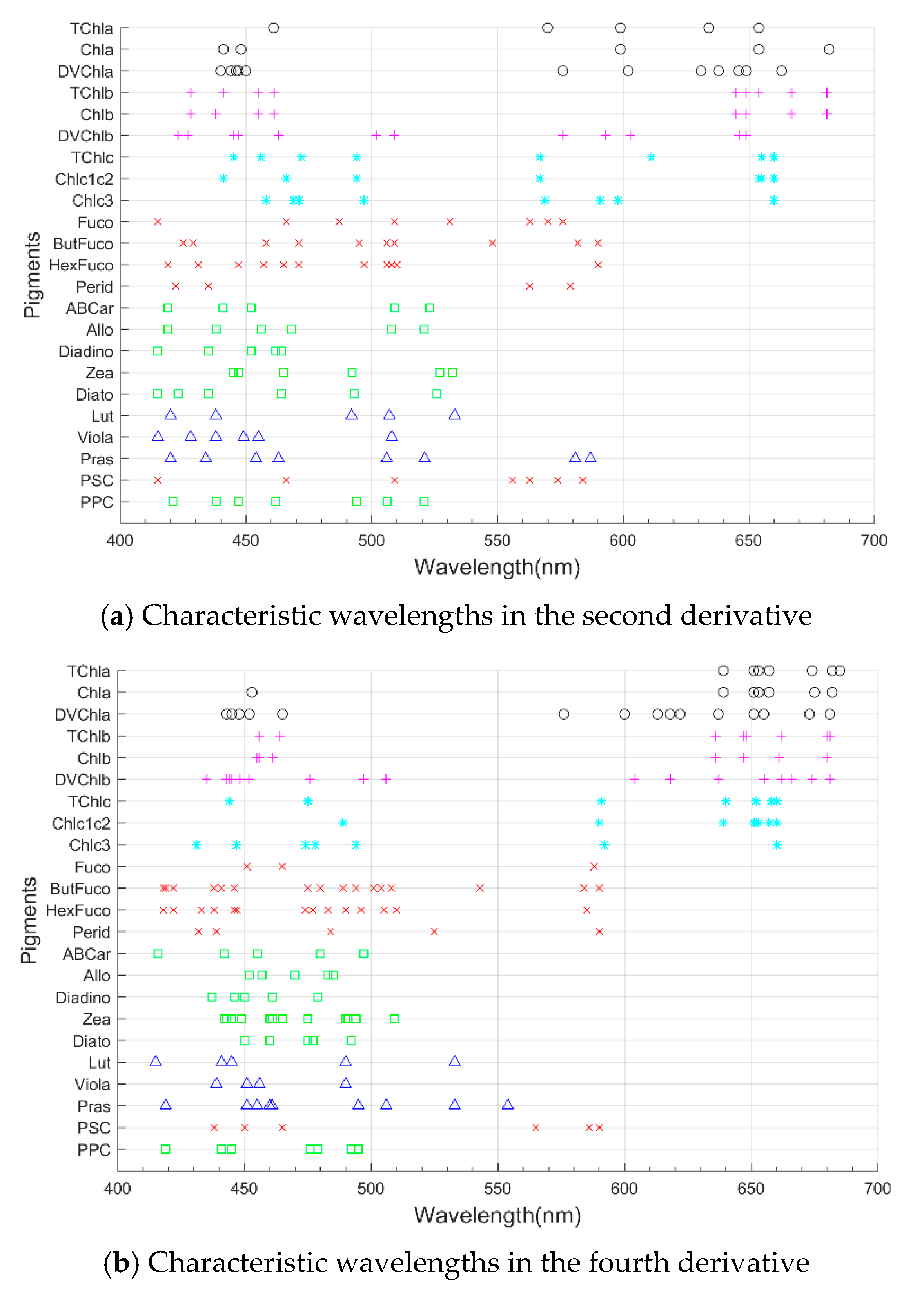
4.1. Characteristic Wavelength Analysis from the ES-SR Method

The characteristic wavelengths of various phytoplankton pigments in a ph and a ph 4 , i.e., the wavelengths of the optimum explanatory variable set, were selected by the ES-SR method (Figure 4). These wavelengths can reflect the important absorption features of the corresponding pigments [30,54], even if these characteristics are hard to detect by traditional methods. For example, the absorptions of Chla at approximately 440 nm and 675 nm, TChlb at approximately 470 nm and 650 nm, TChlc at 467 nm and 630 nm, Fuco in 521–530 nm, Zea in 490–500 nm, and Diadino in 425–500 nm [8,19] have been identified as absorption features important for the identification or inversion of the corresponding pigments in previous studies, and the vast majority of these absorption features can be selected by the ES-SR method.
For most pigments (e.g., TChlb), the positions of many characteristic wavelengths selected by the ES-SR method at a ph are similar to those selected at a ph 4 , and this similarity distribution of characteristic wavelengths from a ph and a ph 4 can indirectly verify the reliability of the ES-SR method (Figure 4). For most pigments, there is also some degree of difference in the location distribution of the characteristic wavelengths selected at a ph and a ph 4 . For example, the ES-SR method selected two explanatory variables of Fuco at 500–530 nm for a ph (Figure 4a), although no explanatory variables were selected in the corresponding interval of a ph 4 (Figure 4b). The ES-SR method selected one explanatory variable of Perid at approximately 480 nm for a ph 4 , and no explanatory variables were obtained in the corresponding interval of a ph . Thus, the second derivative and fourth derivative transformations have advantages in the spectral feature mining of phytoplankton pigments.
In addition, the ES-SR method has a certain degree of offset in the position of the pigment characteristic wavelengths selected for a ph and a ph 4 . For example, the ES-SR method picks the explanatory variable of Chla at 448 nm for a ph , and the explanatory variable picked for a ph 4 is at 453 nm (Figure 4b). The position shifts of the characteristic wavelengths selected by the ES-SR method for a ph and a ph 4 are due to the difference in the mathematical meaning of the derivatives of different orders.
The distribution patterns of the pigment characteristic wavelength positions selected by the ES-SR method for a ph and a ph 4 are relatively similar for pigments of the same class (the same symbols in Figure 4) and more different for pigments of different classes (different symbols in Figure 4).
In summary, the ES-SR method is an effective pigment feature selection method, and the results of its pigment feature selection initially verify the reliability of the method for pigment concentration inversion.

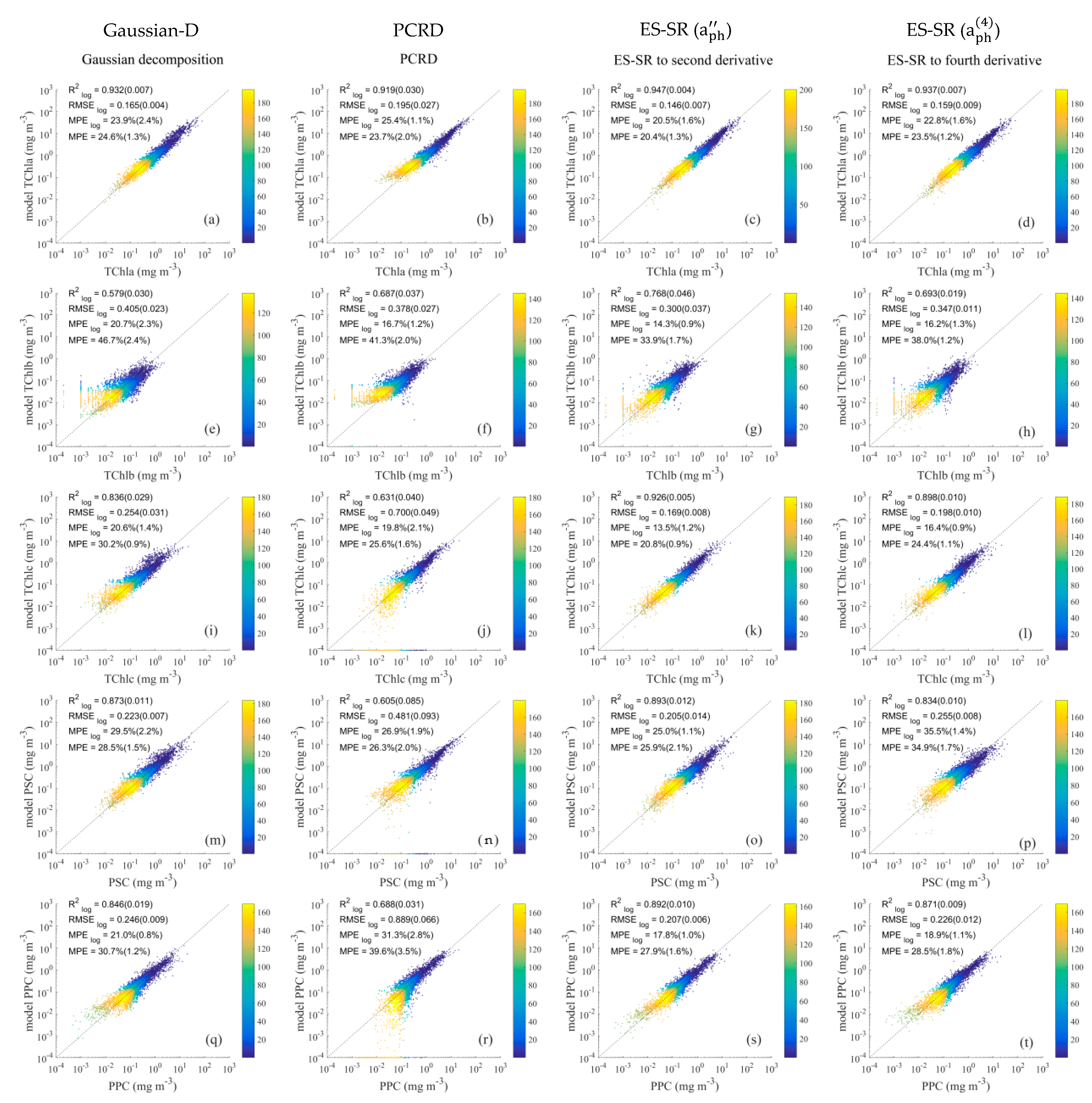
4.2. Result Comparison

To objectively evaluate the uncertainty of the ES-SR method applied to global data, the well-developed Gaussian decomposition method and the promising PCRD method were selected as the comparison methods. The statistical characteristics of the cross-validation results using these inversion methods were compared in detail.

4.2.1. Results of Pigment Group Comparison

The cross-validation results of pigment groups using the Gaussian decomposition method, PCRD method, ES-SR on a ph and ES-SR on a ph 4 are shown in Figure 5. To observe the overall characteristics of the validation results, the calculated negative values are labelled 0.0001 in this study.
The inversion results of the Gaussian decomposition method for TChla, TChlc, PSC and PPC concentrations (Figure 5a,i,m,q) exhibit good accuracy and good evaluation statistics ( R 2 log : 0.836–0.932, RMSE log : 0.165–0.254, MPE log : 20.6–29.5%, MPE : 24.6–30.7%), but the inversion results obtained for TChlb concentrations (Figure 5e) are relatively poor ( R 2 log = 0.579, RMSE log = 0.405, MPE log = 20.7%, MPE = 46.7%). The inversion results of the Gaussian decomposition method for phytoplankton pigment collection show good performance, but their accuracy needs to be further improved. In addition, the Gaussian decomposition method cannot retrieve detailed diagnostic pigments, which are critical for identifying the composition of phytoplankton communities [68] and greatly limit its application potential.
The TChlb, TChlc, PSC and PPC concentration inversion results of the PCRD method (Figure 5b,j,n,r) are less accurate than the results of the Gaussian decomposition method and have a relatively poor statistical evaluation performance ( R 2 log : 0.605–0.688, RMSE log : 0.378–0.889, MPE log : 16.7–31.3%, and MPE : 25.6–41.3%). The TChlc, PSC and PPC concentration inversion results of the PCRD method (Figure 5j,n,r) contain a certain number of negative values which conflict with reality. In addition, when the pigment concentration of the samples is low, the inversion results of the PCRD method are more severely discrete in the plot, and the accuracy of the calculation is significantly lower.
The ES-SR method on a ph is the best method for the inversion of TChla, TChlb, TChlc, PSC and PPC (Figure 5), and its R 2 log values are the highest among those of all inversion methods, with values of 0. 947, 0.768, 0.926, 0.893 and 0.892, respectively, which are significantly higher than those of the Gaussian decomposition method and PCRD method. The RMSE log (0.146–0.300), MPE log (13.5–25.0%), and MPE (20.4–33.9%) values obtained for the inversion results of the ES-SR method on a ph are also significantly lower than those of other methods. The inversion accuracy of the TChlb concentration was the lowest among the inversion accuracies of the five pigment group concentrations retrieved by the ES-SR method on a ph , which may result from the relatively low concentration distribution of TChlb (Table A2) since a lower pigment concentration distribution implies less spectral information. In addition, the inversion results of the ES-SR a ph 4 obtained for pigment group concentrations were similar to those of the ES-SR method on a ph , and the former results are slightly less accurate but mostly higher than the results of the Gaussian decomposition method and PCRD method in accuracy.

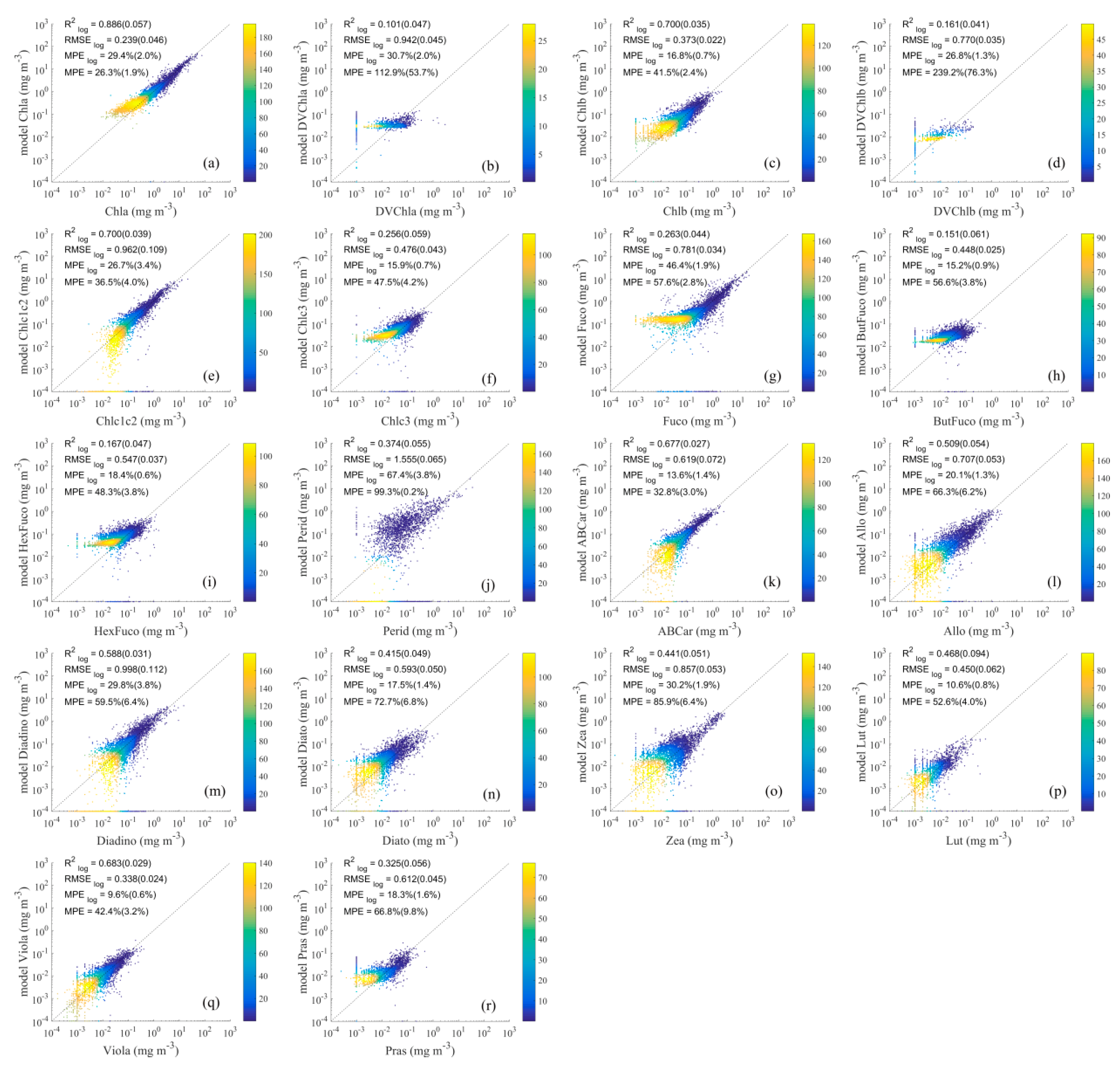
4.2.2. Results of Detailed Pigment Comparison

The cross-validation results of the 18 detailed pigments using the PCRD method, ES-SR on a ph and ES-SR on a ph 4 are shown in Figure 6, Figure 7 and Figure 8.
The results of the detailed pigments obtained using the PCRD method are shown in Figure 6, in which the R 2 log values for Chla, Chlb and Chlc1c2 are greater than 0.7, the values for ABCar, Allo, Diadito, and Viola are greater than 0.5, and the values for the remaining pigments are very low, such as DVChla (0.101), DVChlb (0.161), Chlc3 (0.256), Fuco (0.263), ButFuco (0.151), and HexFuco (0.167). Meanwhile, for the other evaluation statistics of the PCRD method, RMSE log was 0.239–1.555, MPE log was 9.6–67.4% and the MPE was 26.3–239.2%. In addition, the previously mentioned problems with the PCRD method in retrieving pigment group concentrations, i.e., negative inversion results and low inversion accuracy for samples with lower pigment concentrations, still exist or are even more serious, as for DVChla and Perid.
The inversion results of the detailed pigment concentrations obtained using the ES-SR on a ph are shown in Figure 7, where R 2 log is greater than 0.7 for half of the pigments, especially Chla (0.939), Chlc1c2 (0.939), Fuco (0.818), ABCar (0.834), and Diadino (0.799), whose concentration distributions in the ocean are relatively high, and the remaining pigments have R 2 log values greater than 0.5, except for ButFuco (0.454) and Pras (0.464). The reasonable inversion results of the ES-SR method on a ph are also present for other statistical evaluation parameters, such as RMSE log (0.161–0.508), MPE log (8.2–28.5%), and MPE (21.8–64.5%). The inversion results of the ES-SR method on a ph for the concentrations of most pigments are well distributed around the 1:1 line, indicating that the inversion results of this method are mainly affected by some kind of random error, such as measurement noise, and show good performance.
The inversion results of the detailed pigment concentrations obtained using the ES-SR method on a ph 4 are shown in Figure 8, and the evaluated statistical parameters include R 2 log (0.343–0.927), RMSE log (0.177–0.598), MPE log (8.2–40.5%), and MPE (25.6–76.3%). The inversion results of the detailed pigment concentration obtained using the ES-SR method on a ph 4 (Figure 8) were similar to those of the ES-SR method on a ph (Figure 7), and the former method was slightly less accurate but yielded higher accuracy than the PCRD method. In some previous studies, the spectral features of a ph 4 performed better than those of a ph in identifying the major pigments, and the former was less affected by pigment packaging effects [8,19]. However, the ES-SR method on a ph 4 performed slightly worse than the ES-SR method on a ph in this study, possibly because a ph 4 is weaker than a ph in terms of resistance to noise interference.
In summary, by comparing and analysing the validation results of different inversion methods for global ocean water samples, the ES-SR method on a ph is the optimal inversion method for the 18 detailed pigments and has the highest accuracy. The ES-SR method on a ph showed a significant overall improvement in inversion accuracy for the detailed pigments compared to the PCRD method and slightly better performance than the ES-SR method on a ph 4 .

4.3. Effects of Impact Factors on Inversion Methods

To evaluate the robustness of inversion methods and determine the primary cause that influences the method accuracy, the impact of phytoplankton size class and pigment composition on inversion methods was assessed. The Pearson’s correlation (R) values between the absolute values of the relative deviation of the pigment concentrations retrieved using various inversion methods and impact factors (pigment composition and size class) were calculated and are shown in Figure 9 and Figure 10. When the significance level p of R is greater than 0.05, the impact factors have an insignificant influence on the pigment concentration inversion method and are not labelled in the figure. The higher the absolute value of R is, the stronger the influence of the impact factor on the inversion method. When the absolute value of R is small, the influence of the impact factors is not obvious, so this paper focuses on the regular analysis of the impact factors for absolute values of R greater than 0.2.

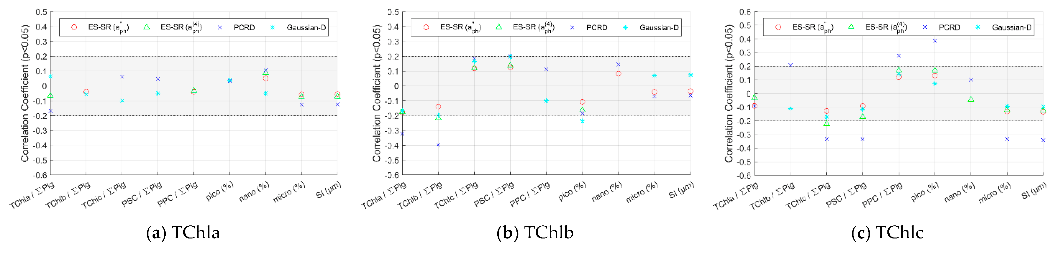
4.3.1. Methods Evaluation for Pigment Groups Based on Impact Factors

The absolute value of R between the inversion results of the ES-SR method on a ph for the five pigment groups and the impact factors is very low overall, and the vast majority are less than 0.2 or not significant (Figure 9). The ES-SR method on a ph shows strong robustness, slightly better than that of the Gaussian decomposition method and that of ES-SR on a ph 4 and significantly better than that of the PCRD method. The absolute values of R between the inversion results of the Gaussian decomposition method and ES-SR on a ph 4 and the impact factors are mostly less than 0.2, and there are a small number of impact factors with an absolute value of R greater than 0.2 for pigments such as TChlb. The absolute values of R between the inversion results of the PCRD method and the impact factors are higher overall. The PCRD method is less resistant to interference than the other methods, and there are impact factors with an absolute value of R greater than 0.3 for some pigments. For example, the PCRD method is obviously influenced by some impact factors for the inversion of TChlc concentration, especially by the proportion of picophytoplankton (R = 0.39), which can be interpreted as follows: TChlc is widely distributed in red algae, which is not a type of picophytoplankton (Table A1). Therefore, the larger the proportion of picophytoplankton in the water sample is, the more interference information and the larger the deviation in the inversion results.

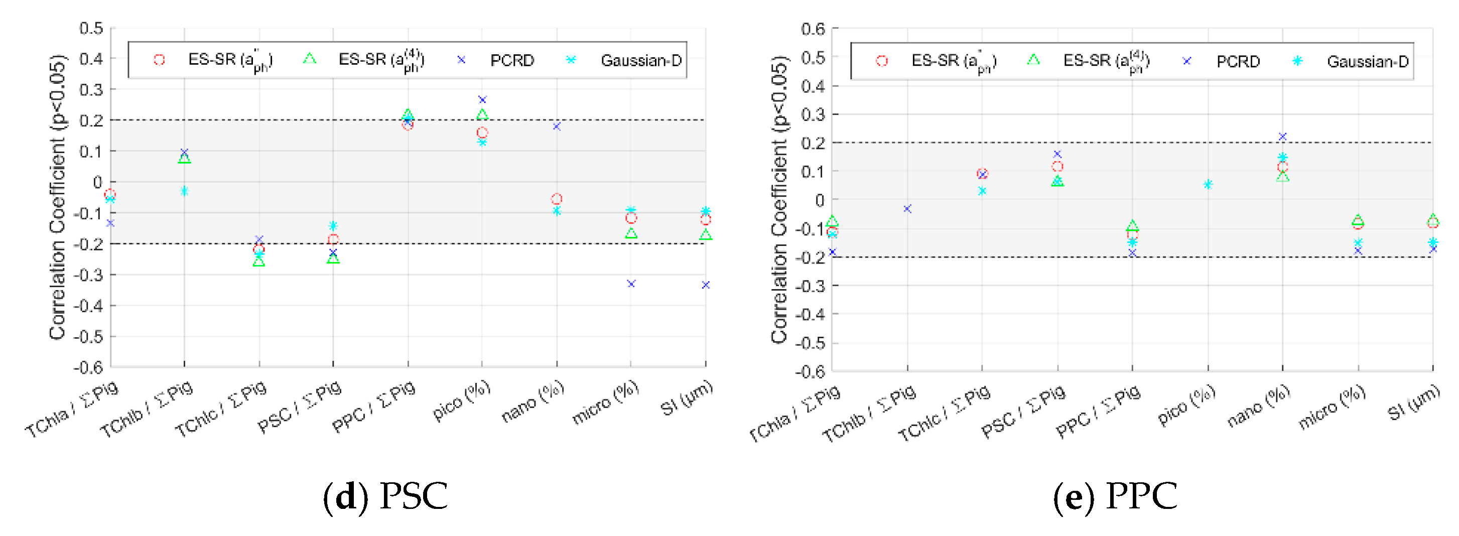
4.3.2. Methods Evaluation for Detailed Pigments Based on Impact Factors

The absolute value of R between the inversion results of the ES-SR method on a ph for the 18 detailed pigments and the impact factors is very low overall, and most are less than 0.2 (Figure 10). The ES-SR method on a ph shows strong robustness, slightly better than that of the ES-SR method on a ph 4 and significantly better than that of the PCRD method. The absolute values of R between the inversion results of the PCRD method and the impact factors are generally high, and some are much greater than 0.2 for various detailed pigments. Their maximum value is mostly the percentage of the corresponding pigment concentration, i.e., the influence of pigment composition on the PCRD method is stronger than that of cell size class. For example, the absolute value of R between the inversion results of the PCRD method for Chlb and the percentage of Chlb concentration is 0.41, which is the highest among the impact factors.
Because the inversion accuracy of the ES-SR method on a ph is better than that of the ES-SR method on a ph 4 , the patterns of the inversion results obtained using the two methods are similar. Therefore, the analysis focused on the pattern of the ES-SR method on a ph influenced by impact factors (Figure 10). For each detailed pigment, the maximum value of the absolute values of R between the inversion results of the ES-SR method on a ph and impact factors is mostly the percentage of the pigment concentration. Thus, the pigment composition influences more than the size class in the performance of the ES-SR method on a ph . For Chla, Chlb, Chlc1c2, Viola, and ABCar, the inversion results of the ES-SR method on a ph have low absolute values of R (<0.2) for most impact factors, so they are less influenced by impact factors (Figure 10). For DVChla, Chlc3, Fuco, ButFuco, HexFuco, Perid, Lut, Allo, Diadino, Diato, Zea, and Pras, the absolute value of R between the inversion results of the ES-SR method on a ph and the percentage of the target pigment itself is higher than that of other impact factors, and its corresponding R value is negative (<−0.2); i.e., the higher the percentage of the target pigment concentration is, the smaller the deviation in the inversion results. However, for DVChlb, there is a difference from the pattern mentioned above. The R value between the inversion results of the ES-SR method on a ph for DVChlb and the percentage of the Chlb concentration is close to 0.3, and its absolute value is the largest among those of the impact factors; i.e., the influence of the percentage of the Chlb concentration is greater than that of the DVChlb concentration, which can be explained as follows. The concentration distribution of Chlb in the ocean is significantly higher than that of DVChlb (Table A2), implying that more Chlb spectral information exists. The correlation between the concentrations of Chlb and DVChlb is extremely low (Figure A1), and the concentrations of the two pigments are independently distributed from each other. The absorption spectral features of Chlb and DVChlb are very similar and difficult to distinguish (Figure 2). Therefore, the inversion of DVChlb concentration is more likely to be affected by Chlb, and the higher the percentage of the Chlb concentration is, the greater the deviation in the DVChlb inversion results. The results in Figure 10 can be well interpreted with high confidence.

5. Conclusions

In this study, a global dataset, including phytoplankton pigment concentrations and hyperspectral data a ph , was comprehensively analysed. A strong correlation between the logarithm of phytoplankton pigment concentrations and the logarithm of the absolute values of a ph and a ph 4 was found, which is critical to the establishment of pigment concentration inversion methods from a ph in global oceans. The stepwise regression method was improved by introducing expert knowledge to assist in variable selection and adding automatic stopping criteria, and the ES-SR method was proposed to retrieve pigment concentrations from a ph and a ph 4 . The ES-SR method can effectively obtain optimum explanatory variable sets, including important absorption features of pigments, and these variables have the potential to be used for pigment concentration inversion.
The performance of the ES-SR method on a ph was verified by method comparison and impact factor evaluation, and the influence law of impact factors on the inversion method was analysed. The inversion accuracy of the ES-SR method on a ph for each pigment was significantly higher than that of the Gaussian decomposition method and that PCRD method, and better evaluation statistics were obtained: R 2 log of 0.454–0.947, RMSE log of 0.146–0.508, MPE log of 8.2–28.5, and an MPE of 20.4–64.5%. The inversion results of the ES-SR method on a ph were significantly less correlated with pigment composition and size class, i.e., less affected, than those of other methods. The pigment composition was correlated more strongly with the results calculated by various pigment inversion methods relative to phytoplankton size class. The above results indicate that the ES-SR method on a ph has relatively high accuracy and powerful robustness and can be applied to the major pigments in global marine waters. The effects of pigment composition on various inversion methods for pigment concentration were generally larger than those of size class, and these effects can be reduced as the performance of the inversion method improves.
Therefore, the ES-SR method on a ph can potentially be used to effectively retrieve pigment concentrations based on hyperspectral optical data from various types of platforms that can observe over diverse temporal and spatial scales within global oceans, and these retrieved pigments can then be further exploited to estimate the phytoplankton community composition and variation, taking advantage of applications such as CHEMTAX [26,27,28]. Nevertheless, for the inversion of some pigment (e.g., Pras) concentrations, the ES-SR method on a ph is still obviously influenced by few impact factors, especially those related to pigment composition. To retrieve pigment concentrations more accurately, it is necessary to collect data from more sea areas and divide the global ocean into provinces based on the geographical distribution of biota or regional absorption characteristics [69,70,71], and an inversion model for each province then needs to be established separately, since there are fewer variations in impact factors within the same province.

Supplementary Materials

The following supporting information can be downloaded at: https://0-www-mdpi-com.brum.beds.ac.uk/article/10.3390/rs14153516/s1, Table S1: The coefficients determined for Equation (3) based on a ph .; Table S2: The coefficients determined for Equation (3) based on a ph 4 .

Author Contributions

Conceptualization, J.T. and T.Z.; methodology, J.T.; software, J.T.; formal analysis, J.T.; writing—original draft preparation, J.T.; writing—review and editing, J.T., T.Z., K.S. and H.G.; visualization, J.T., K.S. and H.G.; supervision, T.Z. All authors have read and agreed to the published version of the manuscript.

Funding

This research was funded by the National Natural Science Foundation of China [grant number 41276041], and NSFC-Shandong Joint Fund for Marine Science Research Centers [grant number U1406405].

Data Availability Statement

Not applicable.

Acknowledgments

The authors are grateful to everyone who worked hard collecting the in situ data and to those who maintained and contributed data to the NASA SeaBASS data archive. We truly appreciate the anonymous reviewers who provided constructive suggestions to improve the quality of this manuscript.

Conflicts of Interest

The authors declare no conflict of interest.

Appendix A. Information on Phytoplankton Pigments

Table A1. Pigments used in this manuscript, corresponding abbreviations and known taxonomic distributions of phytoplankton [9,28,29,32].
AbbreviationPigment (Pigment Group)Taxonomic Distribution (Corresponding Phytoplankton Groups)
TChlaTotal chlorophyll a
(TChla = Chla + DVChla + Chlorophyllide a)
All taxa
Chlachlorophyll aAll taxa, with the exception of some cyanobacteria
DVChlaDivinyl chlorophyll aCyanobacteria, prochlorophytes
TChlbTotal chlorophyll b
(TChlb = Chlb + DVChlb)
Prochlorophytes, cyanobacteria, chlorarachniophytes,
mesostigmatophytes, chlorophytes, prasinophytes, green algae,
euglenophytes, dinoflagellates
Chlbchlorophyll bProchlorophytes, cyanobacteria, chlorarachniophytes,
mesostigmatophytes, chlorophytes, prasinophytes, green algae,
euglenophytes, dinoflagellates
DVChlbDivinyl chlorophyll bProchlorophytes
TChlcTotal chlorophyll c
(TChlc = Chlc1c2 + Chlc3)
All red algae except rhodophytes and eustigmatophytes
Chlc1c2Chlorophylls c1 and c2Diatoms, chrysophytes, cryptophytes, dictyophytes, pelagophytes, raphidophytes, synurophytes, haptophytes, dinoflagellates
Chlc3Chlorophyll c3Diatoms, dictyophytes, pelagophytes, haptophytes, dinoflagellates
FucoFucoxanthinDiatoms, bolidophytes, chrysophytes, dictyophytes, pelagophytes, raphidophytes, silicoflagellates, phaetamniophytes, pinguiophytes, synurophytes, haptophytes, dinoflagellates
ButFuco19′-ButanoyloxyfucoxanthinDiatoms, dictyophytes, raphidophytes, silicoflagellates,
pelagophytes, chrysophytes, dinoflagellates, haptophytes
HexFuco19′-HexanoyloxyfucoxanthinHaptophytes, dinoflagellates
PeridPeridininDinoflagellates (Not all pigmented dinoflagellates contain peridinin.)
ABCarAlpha-beta-carotene
(β, β-carotene + β, ε-carotene)
All taxa
AlloAlloxanthinCryptophytes, dinoflagellates, chlorophytes
DiadinoDiadinoxanthinDiatoms, bolidophytes, dictyophytes, pelagophytes, xanthophytes, haptophytes, dinoflagellates, euglenophytes,
ZeaZeaxanthinCyanobacteria, prochlorophytes, glaucocystophytes, rhodophytes, chrysophytes, eustigmatophytes, pinguiophytes, raphidophytes,
pelagophytes, dinoflagellates, chlorarachniophytes, prasinophytes, chlorophytes, diatoms, dictyophytes
DiatoDiatoxanthinDiatoms, bolidophytes, dictyophytes, pelagophytes, xanthophytes, haptophytes, dinoflagellates, euglenophytes
LutLuteinChlorarachniophytes, chlorophytes, prasinophytes, green algae, Mesostigmatophytes
ViolaViolaxanthinDiatoms, dictyophytes, raphidophytes, synurophytes,
mesostigmatophytes, green algae, prasinophytes, chlorophytes, chlorarachniophytes, dinoflagellates, eustigmatophytes,
chrysophytes
PrasPrasinoxanthinPrasinophytes, dinoflagellates
PSCPhotosynthetic carotenoids
(PSC = Fuco + ButFuco + HexFuco + Perid)
PPCPhotoprotective carotenoids
(PPC = Allo + Diadino + Diato + Zea + ABCar)
Pig_sum
(∑Pig)
The sum of pigments
(Pig_sum = TChla + TChlb + TChlc + PSC + PPC + Lut + Viola + Pras)

Appendix B. Analysis of Research Data

Appendix B.1. Phytoplankton Pigment Concentration Analysis

The characteristics of the 23 pigments in the present study are described in Table A2. In particular, as the formal normality test for sample distribution, the skewness ( Skew ) and kurtosis ( Kurt ) of each pigment concentration were calculated before and after logarithmic transformation, respectively [55,56]. The Skew value and Kurt value of a normal distribution are both zero. A reference of substantial departure from normality is proposed, with an absolute Skew value > 2 or an absolute Kurt value > 4 [55]. Before logarithmic transformation, the absolute Skew value of each pigment is distinctly higher than 2, and the absolute Kurt value of each is much higher than 4, even up to 1249.67. After logarithmic transformation, the absolute values of Skew and Kurt for each pigment are less than the respective reference values of substantial departure from normality, and most of the reference values are very close to zero. TChla, TChlc, PSC and PPC, Chla, Chlc1c2, Fuco, Perid, and Diadino had high average concentrations, with values of 2.44 mg m−3, 0.42 mg m−3, 1.02 mg m−3, 0.45 mg m−3, 2.26 mg m−3, 0.35 mg m−3, 0.75 mg m−3, 0.16 mg m−3, and 0.19 mg m−3; and maximum values of 78.95 mg m−3, 21.87 mg m−3, 37.61 mg m−3, 20.36 mg m−3, 78.04 mg m−3, 21.86 mg m−3, 27.57 mg m−3, 35.53 mg m−3, and 15.13 mg m−3, respectively. The remaining pigments, especially DVChla, DVChlb, Chlc3, ButFuco, Lut, Viola and Pras, had lower concentrations. Therefore, the log-transformed pigment concentration should be used as the dependent variable to make a fairer comparison for the global samples across multiple orders of magnitude when the inversion method is built or evaluated.
Table A2. Descriptive statistics for the phytoplankton pigments. These statistical parameters refer to the minimum (Min), maximum (Max), mean, skewness ( Skew ) and kurtosis ( Kurt ).
PigmentMin (mg m−3)Max (mg m−3)Mean (mg m−3)SkewKurtSkew (log10)Kurt (log10)
Chla078.042.266.1558.68−0.16−0.43
DVChla03.000.0131.151249.670.00−1.40
Chlb02.320.104.0933.40−0.760.52
DVChlb00.190.009.39102.290.40−0.34
Chlc1c2021.860.359.95176.01−0.15−0.35
Chlc300.860.072.4610.56−0.690.55
Fuco027.570.757.0075.02−0.43−0.27
ButFuco00.560.033.7429.77−1.283.79
HexFuco01.570.094.2331.82−0.681.25
Perid035.530.1621.63620.80−0.020.53
ABCar02.830.095.3644.80−0.18−0.01
Allo02.480.066.5162.07−0.35−0.18
Diadino015.130.1913.22283.45−0.290.01
Zea03.020.086.1545.02−0.280.32
Diato01.520.038.04109.17−0.600.43
Lut00.580.0113.21275.38−0.47−0.05
Viola00.410.024.9041.94−0.37−0.08
Pras00.560.016.2984.14−0.28−1.12
TChla0.00978.952.445.8753.73−0.11−0.42
TChlb02.320.113.9130.18−0.770.53
TChlc021.870.429.35160.36−0.30−0.11
PSC037.611.027.1378.85−0.21−0.23
PPC020.360.457.2898.21−0.370.62

Appendix B.2. Correlation Coefficients of Phytoplankton Pigment Concentrations

Spearman’s rank correlation coefficients (Rs), a nonparametric method without the normality assumption, between the concentrations of diverse phytoplankton pigments, are shown in Figure A1. There are strong correlations (Rs > 0.86) among the concentrations of TChla, TChlc, PSC and PPC. Chla, Chlc1c2, Fuco, Perid, and Diadino have large values of Rs (>0.70) with many detailed pigments and have relatively high concentrations in the ocean (Table A2). Chlb, DVChla, DVChlb, ABCar, Allo, ABCar, Viola, and Diato have large values of Rs (>0.70) with few detailed pigments and have relatively low concentrations in the ocean, particularly for DVChla, DVChlb, and Viola (Table A2). These strong correlations among pigments may result in the deviation of calculated values from measured values and increase the difficulty of interpreting the results of inversion methods.
Figure A1. Spearman’s rank correlation coefficients between the concentrations of phytoplankton pigments.
Remotesensing 14 03516 g0a1

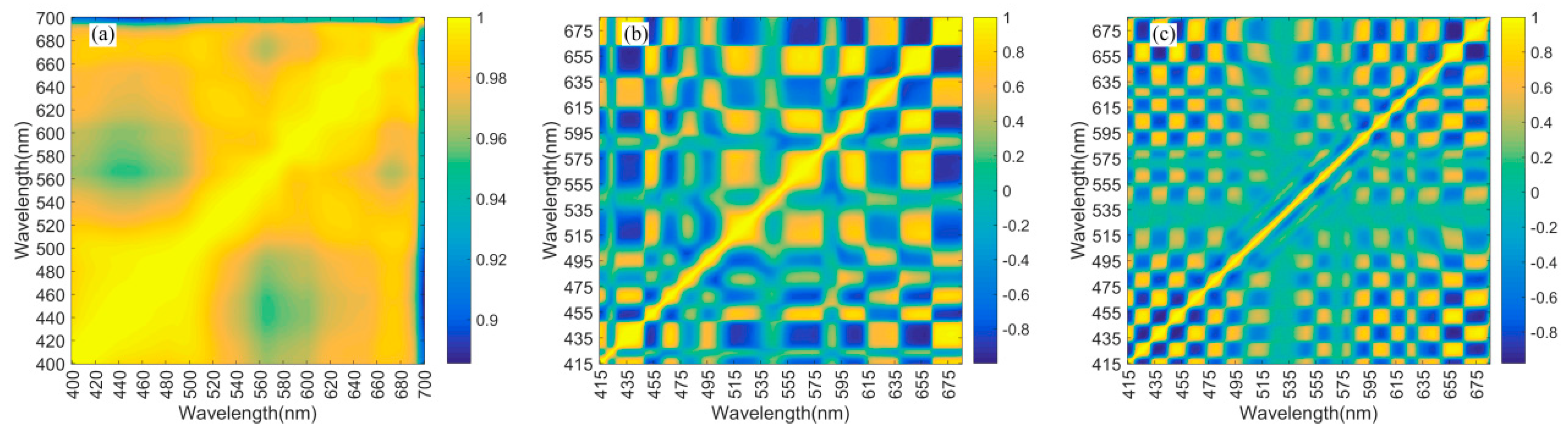
Appendix B.3. Correlation Coefficients of Phytoplankton Absorption and Derivative Spectra

The Spearman’s rank correlation coefficients of spectral wavelengths, related to a ph , a ph and a ph 4 , are shown in Figure A2. For a ph , in the overall spectral range, there are strong correlations between each pair of wavelengths, and the Rs values are all greater than 0.85 (Figure A2a). The strong multicollinearity problems of a ph result in ill-conditioning of the linear systems for modelling. The transformation of the derivative can obviously reduce the correlation between diverse wavelengths, and the higher derivative (Figure A2c) generally obtains smaller values of Rs than the lower-order derivative (Figure A2b). Although ill-conditioning cannot be eliminated, the problem can be mitigated by reducing the dimensions of the explanatory variable set using a reliable data-mining method. The correlations between many closely adjacent bands rapidly drop to extremely low levels after the transformation of the derivative (Figure A2); thus, the adjacent bands with different information can be simultaneously incorporated into explanatory variable sets for modelling.
Figure A2. Rs values of spectral wavelengths related to a ph (a), a ph (b) and a ph 4 (c).
Remotesensing 14 03516 g0a2

Appendix C. Additional Information on Method Evaluation

Appendix C.1. Statistics

Each pigment concentration, calculated by inversion methods, was evaluated with HPLC pigment concentrations by several statistical metrics: the determination coefficient ( R 2 ), the root mean square error ( RMSE ) and the median absolute percentage error ( MPE ). They were computed as follows:
R 2 = i = 1 n y ^ i y ¯ 2 i = 1 n y i y ¯ 2  
RMSE = 1 n i = 1 n ( y ^ i y i ) 2
MPE = median   of   y ^ i y i y i
where y i and y ^ i refer to the measured and retrieved values, respectively; y ¯ is the mean of all retrieved values; and n is the number of samples. R 2 , the RMSE , and the MPE were calculated using the measured and retrieved pigment concentrations in log10 space and abbreviated as R 2 log , RMSE log and MPE log to ensure that the overall performance of global samples, distributed across several orders of magnitude, can be effectively reflected by the statistical metrics. In addition, the MPE was computed using the measured and retrieved pigment concentrations.
To assess the generalization ability of predictive models, 10-fold cross validation was performed to estimate the prediction error of each model [63,64]. The optimal model was finally selected by choosing the one with the minimum loss function within the mean RMSE of the training set and validation set of ten inversion models.

Appendix C.2. Comparison Methods

Appendix C.2.1. Gaussian Decomposition Method

Gaussian functions can determine absorption by individual phytoplankton pigments, and these Gaussian functions can approximately represent the peak locations of absorption by diverse phytoplankton pigments, which have good correlations with the concentrations of pigment groups obtained from HPLC [10,30,33,34,65]. Referring to the study of Chase et al. [10], twelve Gaussian functions were used to decompose a ph using the least square curve-fitting technique, and the parameter varied iteratively with bounds of ±5 nm. The average peak location and standard deviation values of these Gaussian functions were calculated and used to retrieve the Gaussian peak values of all samples. The Gaussian peak values at 676.3 nm, 469.1 nm, 639.8 nm, 521.9 nm and 491.6 nm were used to retrieve the pigment concentrations of TChla, TChlb, TChlc, PSC and PPC, respectively. The optimal linear regression equation for pigment concentrations was established using linear least-squares fitting:
log 10 C i = A ij + B ij   log a gaus λ j
where C i is the log-transformed ith pigment concentration, a gaus λ j is the jth Gaussian peak value, and the coefficients A ij and B ij describe the relationship between the ith pigment concentration and the jth Gaussian peak value inverted from a ph . The concentrations of TChla, TChlb, TChlc, PSC and PPC were calculated using Equation (A4) and used as the results of the Gaussian decomposition method for comparison.

Appendix C.2.2. PCRD Method

There are unique patterns of strong correlations between the results of principal component analysis applied to the derivative of a ph and some phytoplankton pigment concentrations [9,15]. According to the study of Catlett and Siegel [9], the concentrations of phytoplankton pigments in Table A1 were retrieved as a linear sum of contributions from the first derivative spectra ( a ph λ i ) and the second derivative spectra ( a ph λ i ):
p m = i = 1 N [ A m λ i     a ph λ i + B m λ i     a ph λ i ] + C m
where p m is the value of the mth retrieved pigment concentration of phytoplankton, A m λ i and B m λ i are the coefficients of the first and second derivatives of a ph at the ith wavelength λ for the mth pigment concentration, and C m is an intercept. The principal component regression method was used to derive each set of A m λ i and B m λ i to solve the multicollinearity problem [9,66]. The values of a ph λ and a ph λ were standardized to have zero mean and unit variance before computing principal components. The values retrieved by the PCRD method were used for comparison.

Appendix C.3. Impact Factors of the Inversion Method

This paper calculates the ratio of the 23 pigment concentrations listed in Table A1 to the total pigment concentration as the impact factors of pigment composition and the respective contributions of picophytoplankton ( ƒ pico ), nanophytoplankton ( ƒ nano ) and microphytoplankton ( ƒ micro ) to TChla biomass and the pigment-based size index (SI) as the impact factors of size class [8,15,30,31,67]. The fractions of each pigment-derived size class in TChla and SI are calculated as follows:
ƒ micro = 1.41   Fuco + 1.41   Perid / DP
ƒ nano = 0.60   Allo + 0.35   ButFuco + 1.27   HexFuco / DP
ƒ pico = 0.86   Zea + 1.01   TChlb / DP
where pigment abbreviations are described in Table A1 and DP is the sum of the weighted concentrations of seven diagnostic pigments:
DP = 1.41   Fuco + 1.41   Perid + 0.60   Allo + 0.35   ButFuco + 1.27   HexFuco + 0.86   Zea + 1.01   TChlb
SI = 1 × ƒ pico + 5 × ƒ nano + 50 × ƒ micro
where the values 1, 5 and 50 are approximate central values of cell size (in units of μm) for the pico-, nano- and microphytoplankton classes, respectively.

References

  1. Behrenfeld, M.J.; Boss, E.; Siegel, D.A.; Shea, D.M. Carbon-based ocean productivity and phytoplankton physiology from space. Glob. Biogeochem. Cycles 2005, 19, GB1006. [Google Scholar] [CrossRef]
  2. Le Quéré, C.L.; Harrison, S.P.; Prentice, I.C.; Buitenhuis, E.T.; Aumont, O.; Bopp, L.; Claustre, H.; Cunha, L.C.D.; Geider, R.; Giraud, X.; et al. Ecosystem dynamics based on plankton functional types for global ocean biogeochemistry models. Glob. Chang. Biol. 2005, 11, 2016–2040. [Google Scholar]
  3. Nair, A.; Sathyendranath, S.; Platt, T.; Morales, J.; Stuart, V.; Forget, M.-H.; Devred, E.; Bouman, H. Remote sensing of phytoplankton functional types. Remote Sens. Environ. 2008, 112, 3366–3375. [Google Scholar] [CrossRef]
  4. Muller-Karger, F.; Kavanaugh, M.T.; Montes, E.; Balch, W.M.; Breitbart, M.; Chavez, F.P.; Doney, S.C.; Johns, E.M.; Letelier, R.M.; Lomas, M.W.; et al. A Framework for a Marine Biodiversity Observing Network within Changing Continental Shelf Seascapes. Oceanography 2014, 27, 18–23. [Google Scholar] [CrossRef] [Green Version]
  5. Edwards, K.F.; Thomas, M.K.; Klausmeier, C.A.; Litchman, E. Phytoplankton growth and the interaction of light and temperature: A synthesis at the species and community level. Limnol. Oceanogr. 2016, 61, 1232–1244. [Google Scholar] [CrossRef] [Green Version]
  6. Chase, A.P.; Boss, E.; Cetinić, I.; Slade, W. Estimation of phytoplankton accessory pigments from hyperspectral reflectance spectra: Toward a global algorithm. J. Geophys. Res. Ocean. 2017, 122, 9725–9743. [Google Scholar] [CrossRef]
  7. IOCCG. Phytoplankton Functional Types from Space; Sathyendranath, S., Ed.; Reports of the International Ocean-Colour Coordinating Group, No. 15; IOCCG: Dartmouth, NS, Canada, 2014. [Google Scholar]
  8. Lorenzoni, L.; Toro-Farmer, G.; Varela, R.; Guzman, L.; Rojas, J.; Montes, E.; Muller-Karger, F. Characterization of phytoplankton variability in the Cariaco Basin using spectral absorption, taxonomic and pigment data. Remote Sens. Environ. 2015, 167, 259–268. [Google Scholar] [CrossRef]
  9. Catlett, D.; Siegel, D.A. Phytoplankton pigment communities can be modeled using unique relationships with spectral absorption signatures in a dynamic coastal environment. J. Geophys. Res. 2018, 123, 246–264. [Google Scholar] [CrossRef] [Green Version]
  10. Chase, A.; Boss, E.; Zaneveld, R.; Bricaud, A.; Claustre, H.; Ras, J.; Dall’Olmo, G.; Westberry, T.K. Decomposition of in situ particulate absorption spectra. Methods Oceanogr. 2013, 7, 110–124. [Google Scholar] [CrossRef]
  11. Bracher, A.; Bouman, H.A.; Brewin, R.J.W.; Bricaud, A.; Brotas, V.; Ciotti, A.M.; Clementson, L.; Devred, E.; Di Cicco, A.; Dutkiewicz, S.; et al. Obtaining Phytoplankton Diversity from Ocean Color: A Scientifific Roadmap for Future Development. Front. Mar. Sci. 2017, 4, 55. [Google Scholar] [CrossRef] [Green Version]
  12. Liu, Y.; Boss, E.; Chase, A.; Xi, H.; Zhang, X.; Röttgers, R.; Pan, Y.; Bracher, A. Retrieval of Phytoplankton Pigments from Underway Spectrophotometry in the Fram Strait. Remote Sens. 2019, 11, 318. [Google Scholar] [CrossRef] [Green Version]
  13. Dickey, T.; Lewis, M.; Chang, G. Optical oceanography: Recent advances and future directions using global remote sensing and in situ observations. Rev. Geophys. 2006, 44, RG1001. [Google Scholar] [CrossRef] [Green Version]
  14. Lee, Z.; Shang, S.; Hu, C.; Zibordi, G. Spectral interdependence of remote-sensing reflectance and its implications on the design of ocean color satellite sensors. Appl. Opt. 2014, 53, 3301–3310. [Google Scholar] [CrossRef]
  15. Uitz, J.; Stramski, D.; Reynolds, R.A.; Dubranna, J. Assessing phytoplankton community composition from hyperspectral measurements of phytoplankton absorption coefficient and remote-sensing reflectance in open-ocean environments. Remote Sens. Environ. 2015, 171, 58–74. [Google Scholar] [CrossRef]
  16. Garver, S.A.; Siegel, D.A. Inherent optical property inversion of ocean color spectra and its biogeochemical interpretation: 1. Time series from the Sargasso Sea. J. Geophy. Res. 1997, 102, 18607–18625. [Google Scholar] [CrossRef]
  17. Lee, Z.; Carder, K.L. Absorption spectrum of phytoplankton pigments derived from hyperspectral remote-sensing reflectance. Remote Sens. Environ. 2004, 89, 361–368. [Google Scholar] [CrossRef]
  18. Isada, T.; Hirawake, T.; Kobayashi, T.; Nosaka, Y.; Natsuike, M.; Imai, I.; Suzuki, K.; Saitoh, S.-I. Hyperspectral optical discrimination of phytoplankton community structure in Funka Bay and its implications for ocean color remote sensing of diatoms. Remote Sens. Environ. 2015, 159, 134–151. [Google Scholar] [CrossRef]
  19. Bidigare, R.R.; Morrow, J.H.; Kiefer, D.A. Derivative analysis of spectral absorption by photosynthetic pigments in the western Sargasso Sea. J. Mar. Res. 1989, 47, 323–341. [Google Scholar] [CrossRef]
  20. Staehr, P.A.; Cullen, J.J. Detection of Karenia mikimotoi by spectral absorption signatures. J. Plankton Res. 2003, 25, 1237–1249. [Google Scholar] [CrossRef]
  21. Devred, E.; Sathyendranath, S.; Stuart, V.; Maass, H.; Ulloa, O.; Platt, T. A two-component model of phytoplankton absorption in the open ocean: Theory and applications. J. Geophys. Res. 2006, 111, C03011. [Google Scholar] [CrossRef]
  22. Barlow, R.; Kyewalyanga, M.; Sessions, H.; van den Berg, M.; Morris, T. Phytoplankton pigments, functional types, and absorption properties in the Delagoa and Natal Bights of the Agulhas ecosystem. Estuar. Coast. Shelf Sci. 2008, 80, 201–211. [Google Scholar] [CrossRef]
  23. Moisan, J.R.; Moisan, T.A.H.; Linkswiler, M.A. An inverse modeling approach to estimating phytoplankton pigment concentrations from phytoplankton absorption spectra. J. Geophys. Res. 2011, 116, C09018. [Google Scholar] [CrossRef] [Green Version]
  24. Xi, H.; Hieronymi, M.; Röttgers, R.; Krasemann, H.; Qiu, Z. Hyperspectral Differentiation of Phytoplankton Taxonomic Groups: A Comparison between Using Remote Sensing Reflectance and Absorption Spectra. Remote Sens. 2015, 7, 14781–14805. [Google Scholar] [CrossRef] [Green Version]
  25. Organelli, E.; Nuccio, C.; Lazzara, L.; Uitz, J.; Bricaud, A.; Massi, L. On the discrimination of multiple phytoplankton groups from light absorption spectra of assemblages with mixed taxonomic composition and variable light conditions. Appl. Opt. 2017, 56, 3952–3968. [Google Scholar] [CrossRef] [Green Version]
  26. Mackey, M.D.; Mackey, D.J.; Higgins, H.W.; Wright, S.W. CHEMTAX—A program for estimating class abundances from chemical markers: Application to HPLC measurements of phytoplankton. Mar. Ecol. Prog. Ser. 1996, 144, 265–283. [Google Scholar] [CrossRef] [Green Version]
  27. Latasa, M. Improving estimations of phytoplankton class abundances using CHEMTAX. Mar. Ecol. Proj. Ser. 2007, 329, 13–21. [Google Scholar] [CrossRef] [Green Version]
  28. Sañé, E.; Valente, A.; Fatela, F.; Cabral, M.C.; Beltrán, C.; Drago, T. Assessment of sedimentary pigments and phytoplankton determined by CHEMTAX analysis as biomarkers of unusual upwelling conditions in summer 2014 off the SE coast of Algarve. J. Sea Res. 2019, 146, 33–45. [Google Scholar] [CrossRef]
  29. Jeffrey, S.W.; Mantoura, R.F.C.; Wright, S.W. Phytoplankton Pigments in Oceanography: Guidelines to Modern Methods, 1st ed.; UNESCO: Paris, France, 1997. [Google Scholar]
  30. Bricaud, A.; Claustre, H.; Ras, J.; Oubelkheir, K. Natural variability of phytoplanktonic absorption in oceanic waters: Influence of the size structure of algal populations. J. Geophys. Res. 2004, 109, C11010. [Google Scholar] [CrossRef]
  31. Uitz, J.; Claustre, H.; Morel, A.; Hooker, S.B. Vertical distribution of phytoplankton communities in open ocean: An assessment based on surface chlorophyll. J. Geophy. Res. 2006, 111, C08005. [Google Scholar] [CrossRef]
  32. Roy, S.; Llewellyn, C.; Egeland, E.S.; Johnsen, G. Phytoplankton Pigments: Characterization, Chemotaxonomy and Applications in Oceanography, 1st ed.; Cambridge University Press: Cambridge, UK, 2011. [Google Scholar]
  33. Hoepffner, N.; Sathyendranath, S. Determination of the major groups of phytoplankton pigments from the absorption spectra of total particulate matter. J. Geophys. Res. 1993, 98, 22789–22803. [Google Scholar] [CrossRef]
  34. Wang, G.; Lee, Z.; Mouw, C.B. Concentrations of Multiple Phytoplankton Pigments in the Global Oceans Obtained from Satellite Ocean Color Measurements with MERIS. Appl. Sci. 2018, 8, 2678. [Google Scholar] [CrossRef] [Green Version]
  35. Moisan, T.A.; Moisan, J.R.; Linkswiler, M.A.; Steinhardt, R.A. Algorithm development for predicting biodiversity based on phytoplankton absorption. Cont. Shelf Res. 2013, 55, 17–28. [Google Scholar] [CrossRef]
  36. Kirkpatrick, G.J.; Millie, D.F.; Moline, M.A.; Schofield, O. Optical Discrimination of a Phytoplankton Species in Natural Mixed Populations. Limnol. Oceanogr. 2000, 45, 467–471. [Google Scholar] [CrossRef]
  37. Aguirre-Gómez, R.; Weeks, A.R.; Boxall, S. The identification of phytoplankton pigments from absorption spectra. Int. J. Remote Sens. 2001, 22, 315–338. [Google Scholar] [CrossRef]
  38. Craig, S.E.; Lohrenz, S.E.; Lee, Z.; Mahoney, K.L.; Kirkpatrick, G.J.; Schofield, O.M.; Steward, R.G. Use of hyperspectral remote sensing reflectance for detection and assessment of the harmful alga, Karenia brevis. Appl. Opt. 2006, 45, 5414–5425. [Google Scholar] [CrossRef]
  39. Lubac, B.; Loisel, H.; Guiselin, N.; Astoreca, R.; Artigas, L.F.; Mériaux, X. Hyperspectral and multispectral ocean color inversions to detect Phaeocystis globosa blooms in coastal waters. J. Geophys. Res. 2008, 113, C06026. [Google Scholar]
  40. Torrecilla, E.; Piera, J.; Vilasec, M. Derivative analysis of hyperspectral oceanographic data. In Advances in Geoscience and Remote Sensing; Jedlovec, G., Ed.; IntechOpen: London, UK, 2009; pp. 597–618. [Google Scholar]
  41. Torrecilla, E.; Stramski, D.; Reynolds, R.A.; Millán-Núñez, E.; Piera, J. Cluster analysis of hyperspectral optical data for discriminating phytoplankton pigment assemblages in the open ocean. Remote Sens. Environ. 2011, 115, 2578–2593. [Google Scholar] [CrossRef] [Green Version]
  42. Wolanin, A.; Soppa, M.; Bracher, A. Investigation of Spectral Band Requirements for Improving Retrievals of Phytoplankton Functional Types. Remote Sens. 2016, 8, 871. [Google Scholar] [CrossRef] [Green Version]
  43. Bidigare, R.R.; Ondrusek, M.E.; Morrow, J.H.; Kiefer, D.A. In-vivo absorption properties of algal pigments. Ocean Opt. X 1990, 1302, 290–302. [Google Scholar]
  44. Robinson, C.M.; Huot, Y.; Schuback, N.; Ryan-Keogh, T.J.; Thomalla, S.J.; Antoine, D. High latitude Southern Ocean phytoplankton have distinctive bio-optical properties. Opt. Express 2021, 29, 21084. [Google Scholar] [CrossRef]
  45. Allali, K.; Bricaud, A.; Claustre, H. Spatial variations in the chlorophyll-specific absorption coefficients of phytoplankton and photosynthetically active pigments in the equatorial Pacific. J. Geophys. Res. 1997, 102, 12413–12423. [Google Scholar] [CrossRef]
  46. Stuart, V.; Sathyendranath, S.; Platt, T.; Maass, H.; Irwin, B.D. Pigments and species composition of natural phytoplankton populations: Effect on the absorption spectra. J. Plankton Res. 1998, 20, 187–217. [Google Scholar] [CrossRef] [Green Version]
  47. Whittingham, M.J.; Stephens, P.A.; Bradbury, R.B.; Freckleton, R.P. Why do we still use stepwise modelling in ecology and behaviour? J. Anim. Ecol. 2006, 75, 1182–1189. [Google Scholar] [CrossRef]
  48. Prost, L.; Makowski, D.; Jeuffroy, M.-H. Comparison of stepwise selection and Bayesian model averaging for yield gap analysis. Ecol. Model. 2008, 219, 66–76. [Google Scholar] [CrossRef]
  49. Smith, D. Step away from stepwise. J. Big Data 2018, 5, 32. [Google Scholar] [CrossRef]
  50. Werdell, P.J.; Bailey, S.; Fargion, G.; Pietras, C.; Knobelspiesse, K.; Feldman, G.; McClain, C. Unique data repository facilitates ocean color satellite validation. Eos Trans. Am. Geophys. Union 2003, 84, 377–387. [Google Scholar] [CrossRef]
  51. Hirata, T.; Aiken, J.; Hardman-Mountford, N.; Smyth, T.J.; Barlow, R.G. An absorption model to determine phytoplankton size classes from satellite ocean colour. Remote Sens. Environ. 2008, 112, 3153–3159. [Google Scholar] [CrossRef]
  52. Specific Criteria of SeaBASS Data. Available online: https://seabass.gsfc.nasa.gov (accessed on 30 December 2018).
  53. Kishino, M.; Takahashi, M.; Okami, N.; Ichimura, S. Estimation of the Spectral Absorption Coefficients of Phytoplankton in the Sea. Bull. Mar. Sci. 1985, 37, 634–642. [Google Scholar]
  54. Clementson, L.A.; Wojtasiewicz, B. Dataset on the in vivo absorption characteristics and pigment composition of various phytoplankton species. Data Brief 2019, 25, 104020. [Google Scholar] [CrossRef]
  55. Kim, T.; White, H. On More Robust Estimation of Skewness and Kurtosis: Simulation and Application to the S&P500 Index; Department of Economics, UCSD, UC: San Diego, CA, USA, 2003. [Google Scholar]
  56. Kim, H.-Y. Statistical notes for clinical researchers: Assessing normal distribution (2) using skewness and kurtosis. Restor. Dent. Endod. 2013, 38, 52–54. [Google Scholar] [CrossRef]
  57. Calude, C.S.; Longo, G. The Deluge of Spurious Correlations in Big Data. Found. Sci. 2016, 22, 595–612. [Google Scholar] [CrossRef] [Green Version]
  58. Ginzburg, L.R.; Jensen, C.X.J. Rules of thumb for judging ecological theories. Trends Ecol. Evol. 2004, 19, 121–126. [Google Scholar] [CrossRef]
  59. Guthery, F.S.; Brennan, L.A.; Peterson, M.J.; Lusk, J.J. Information theory in wildlife science: Critique and viewpoint. J. Wildl. Manag. 2005, 69, 457–465. [Google Scholar] [CrossRef]
  60. Finnoff, W.; Hergert, F.; Zimmermann, H.G. Improving model selection by nonconvergent methods. Neural Netw. 1993, 6, 771–783. [Google Scholar] [CrossRef]
  61. Prechelt, L. Automatic early stopping using cross validation: Quantifying the criteria. Neural Netw. 1998, 11, 761–767. [Google Scholar] [CrossRef] [Green Version]
  62. Dodge, J.; Ilharco, G.; Schwartz, R.; Farhadi, A.; Hajishirzi, H.; Smith, N. Fine-Tuning Pretrained Language Models: Weight Initializations, Data Orders, and Early Stopping. arXiv 2020, arXiv:2002.06305. [Google Scholar]
  63. Simon, R. Resampling strategies for model assessment and selection. In Fundamentals of Data Mining in Genomics and Proteomics; Dubitzky, W., Granzow, M., Berrar, D., Eds.; Springer: Boston, MA, USA, 2007; pp. 173–186. [Google Scholar]
  64. Berrar, D. Cross-Validation. In Encyclopedia of Bioinformatics and Computational Biology; Ranganathan, S., Gribskov, M., Nakai, K., Schönbach, C., Eds.; Elsevier Inc.: Cambridge, UK, 2019; pp. 542–545. [Google Scholar]
  65. Hoepffner, N.; Sathyendranath, S. Effect of pigment composition on absorption properties of phytoplankton. Mar. Ecol. Prog. Ser. 1991, 73, 11–23. [Google Scholar] [CrossRef]
  66. Massy, W.F. Principal components regression in exploratory statistical research. J. Am. Stat. Assoc. 1965, 60, 234–256. [Google Scholar] [CrossRef]
  67. Vidussi, F.; Claustre, H.; Manca, B.B.; Luchetta, A.; Marty, J.-C. Phytoplankton pigment distribution in relation to upper thermocline circulation in the eastern Mediterranean Sea during winter. J. Geophy. Res. 2001, 106, 19939–19956. [Google Scholar] [CrossRef]
  68. Higgins, H.W.; Wright, S.W.; Schlüter, L. Quantitative interpretation of chemotaxonomic pigment data. In Phytoplankton Pigments: Characterization, Chemotaxonomy and Applications in Oceanography; Roy, S., Llewellyn, C., Egeland, E., Johnsen, G., Eds.; Cambridge University Press: Cambridge, UK, 2011; pp. 257–313. [Google Scholar]
  69. Suzuki, K.; Kishino, M.; Sasaoka, K.; Saitoh, S.; Saino, T. ChlorophylI-specific absorption coefficients and pigments of phytoplankton off Sanriku, Northwestern North Pacific. J. Oceanogr. 1998, 54, 517–526. [Google Scholar] [CrossRef]
  70. Longhurst, A.R. Ecological Geography of the Sea, 2nd ed.; Academic Press: New York, USA, 2007. [Google Scholar]
  71. Blondeau-Patissier, D.; Gower, J.F.R.; Dekker, A.G.; Phinn, S.R.; Brando, V.E. A review of ocean color remote sensing methods and statistical techniques for the detection, mapping and analysis of phytoplankton blooms in coastal and open oceans. Prog. Oceanogr. 2014, 123, 123–144. [Google Scholar] [CrossRef] [Green Version]
Figure 1. Location of the study area with sampling stations. The institutions providing data were the Alfred-Wegener-Institute Helmholtz Centre for Polar and Marine Research (AWI), Bowdoin College (BOWDOIN), Commonwealth Scientific and Industrial Research Organization (CSIRO), NASA Goddard Space Flight Center (NASA GSFC), University of California, San Diego Scripps Institution of Oceanography (SIO), University of California, Santa Barbara (UCSB), University of Massachusetts Dartmouth (UMASS D), University of Maryland (UMD), University of South Florida (USF) and Woods Hole Oceanography Institute (WHOI).
Remotesensing 14 03516 g001
Figure 2. In vivo weight-specific absorption spectra of the main pigments, a*. The same colour represents the same type of pigments. Absorption spectra of primary photosynthetic and photoprotective carotenoids are shown in red and green, respectively. See Table A1 for details on pigment categories.
Remotesensing 14 03516 g002
Figure 3. Pearson’s correlation coefficients between the logarithm of phytoplankton pigment concentrations and the logarithm of the absolute values of a ph (a,c,e,g) and a ph 4 (b,d,f,h). Pigments are separated according to the type of pigments (Table A1 and Figure 2) as (a,b) pigment groups, (c,d) chlorophylls, (e,f) photosynthetic carotenoids and (g,h) other carotenoids.
Remotesensing 14 03516 g003
Figure 4. Characteristic wavelengths of pigments in a ph (a) and a ph 4 (b) selected by the ES-SR method. The same symbol represents the same type of pigments. Where circles represent chlorophyll a, plus signs represent chlorophyll b, asterisks represent chlorophyll c, forks represent photosynthetic carotenoids, squares represent photoprotective carotenoids, and triangles represent other carotenoids.
Remotesensing 14 03516 g004
Figure 5. Comparison of phytoplankton pigment group values retrieved using the Gaussian decomposition method (a,e,i,m,q), PCRD method (b,f,j,n,r), ES-SR on a ph (c,g,k,o,s) and ES-SR on a ph 4 (d,h,l,p,t) with measured values. The horizontal axis represents measured pigment concentrations, and the vertical axis represents estimated pigment concentrations. The dashed line is a one-to-one line. The colour scale represents the density.
Remotesensing 14 03516 g005
Figure 6. Comparison of detailed phytoplankton pigment values retrieved using the PCRD method (ar) with measured values. The horizontal axis represents measured pigment concentrations, and the vertical axis represents estimated pigment concentrations. Dashed lines are one-to-one lines. The colour scale represents the density.
Remotesensing 14 03516 g006
Figure 7. Comparison of detailed phytoplankton pigment values retrieved using the ES-SR method on a ph (ar) with measured values. The horizontal axis represents measured pigment concentrations, and the vertical axis represents estimated pigment concentrations. The dashed lines are the one-to-one lines. The colour scale represents the density.
Remotesensing 14 03516 g007
Figure 8. Comparison of detailed phytoplankton pigment values retrieved using the ES-SR method on a ph 4 (ar) with measured values. The horizontal axis represents measured pigment concentrations, and the vertical axis represents estimated pigment concentrations. The dashed lines are the one-to-one lines. The colour scale represents the density.
Remotesensing 14 03516 g008
Figure 9. Pearson’s correlation coefficients between the absolute values of the relative deviation of pigment group concentrations retrieved from the inversion methods and impact factors. Only the values of the correlation coefficient with a significance level p less than 0.05 are indicated. The absolute value of the correlation coefficient in the shaded area is less than 0.2.
Remotesensing 14 03516 g009aRemotesensing 14 03516 g009b
Figure 10. Pearson’s correlation coefficients between the absolute values of the relative deviation in retrieved detailed pigment concentrations from inversion methods and impact factors. Only the values of the correlation coefficient with a significance level p less than 0.05 are indicated. The absolute value of the correlation coefficient in the shaded area is less than 0.2.
Remotesensing 14 03516 g010aRemotesensing 14 03516 g010b
Table 1. Information about the datasets selected from global oceans.
InstitutionTimeSize (N)Depth (m)
AWI2009–20122810–12
BOWDOIN2011–2011260.5–10
CSIRO1997–20106290–150
NASA GSFC2005–20149060–140
SIO2004–20088890–200
UCSB2003–20178030–150
UMASS D2008–2008161–30
UMD1996–20073280–80
USF2012–2016480.5–30
WHOI2006–20146780–40
Table 2. Characteristic wavelength range for retrieving pigment concentrations using derivative transformation of phytoplankton absorption spectra.
Pigment (Pigment Group)Wavelength (nm)
TChla, Chla, DVChla415–475, 570–685
TChlb, Chlb, DVChlb415–515, 575–685
TChlc, Chlc1c2, Chlc3415–505, 538–660
PSC, Fuco, ButFuco, HexFuco, Perid415–590
PPC, Allo, Diadino, Diato, Zea, ABCar, Lut, Viola415–535
Pras415–560
Publisher’s Note: MDPI stays neutral with regard to jurisdictional claims in published maps and institutional affiliations.

