Article

An Improved QAA-Based Method for Monitoring Water Clarity of Honghu Lake Using Landsat TM, ETM+ and OLI Data

1
Key Laboratory for Environment and Disaster Monitoring and Evaluation, Innovation Academy for Precision Measurement Science and Technology, Chinese Academy of Sciences, Wuhan 430077, China
2
University of Chinese Academy of Sciences, Beijing 100049, China
*
Author to whom correspondence should be addressed.
Remote Sens. 2022, 14(15), 3798; https://0-doi-org.brum.beds.ac.uk/10.3390/rs14153798
Submission received: 27 May 2022 / Revised: 24 July 2022 / Accepted: 3 August 2022 / Published: 6 August 2022
(This article belongs to the Special Issue Optical Remote Sensing for Surface Water Parameters Retrieval)

Abstract

:
Secchi disk depth (ZSD) is used to quantify water clarity as an important water-quality parameter, and one of the most used mechanistic models for ZSD is the quasi-analytical algorithm (QAA), of which the latest version is QAA_v6. There are two models in QAA for clear and turbid waters (referred to as QAA_clear and QAA_turbid). QAA_v6 switches between the two models by setting a threshold value for the remote sensing reflectance (Rrs, sr−1) at the selected reference band of 656 nm. However, some researchers found that this reference band or the threshold value does not apply to many turbid inland lakes. In Honghu Lake, the Rrs (656) (Rrs at 656 nm) in the whole lake is less than 0.0015 sr−1; therefore, only QAA_turbid can be applied. Moreover, we found that QAA_clear resulted in overestimation while QAA_turbid resulted in significant underestimations. The waters of inland lakes usually continuously vary between clear and turbid water. We proposed a hypothesis that QAA_turbid and QAA_clear transition evenly, rather than being distinguished by one threshold value, and we developed a model that combined QAA_clear and QAA_turbid according to our assumption. This model simulated the process of continuous change in water clarity. The results showed that our model had a better performance with an RMSE that reduced from 0.5 to 0.28, an MAE that reduced from 0.43 to 0.21, and bias that reduced from −0.4 to −0.05 m compared with QAA_v6. We applied QAA_Honghu to Landsat TM, ETM+, and OLI data and obtained 205 ZSD maps with high spatial resolution in Honghu Lake. The results were consistent with the existing in situ measurements. From 1987–2020, the ZSD results of Honghu Lake showed an overall downward trend and a distinct seasonal pattern.

Graphical Abstract

1. Introduction

Water clarity is an important water-quality parameter that can affect the transmission of light in the water and thus the growth of aquatic vegetation. Secchi disk depth is an important indicator to quantify water clarity. It is closely related to phytoplankton concentration and water eutrophication [1]. The use of a Secchi disk is the simplest and lowest-cost water-quality measurement. Over the past 100 years, more than a million ZSD measurements have been made in marine and inland waters [2].
Traditional studies have analyzed the variation characteristics of the ZSD through many sampling data. Such studies require a large number of sites and are costly. Moreover, this analysis is not spatially continuous. Due to the low cost and high efficiency, there have been many studies on monitoring water clarity through remote sensing [3,4,5]. Most of this research uses two methods. The first one is to derive the ZSD by empirical methods such as regression arithmetic [6] and machine learning [7]. This method is only applicable to waters that are similar to those for which the algorithm was developed, due to the nature of regression. In addition, the lack of measured data will cause greater error [8,9,10]. The second method is the semi-analytical algorithm based on solutions to the radiative transfer equation [11,12].
Lee proposed a new quasi-analytical algorithm based on underwater visibility theory [13]. QAA is a mechanistic model that derives the total absorption coefficient a (λ), total backscattering coefficient bb (λ), and diffuse attenuation coefficient Kd (λ) from Rrs (λ). This algorithm has been applied in many waters around the world for various satellite sensors [14,15,16,17]. Yin et al. successfully applied QAA to Landsat TM and OLI data and observed the water clarity changes in Taihu Lake over 36 years [17]. However, this research did not change the QAA, so further improvements are significant for lakes with complex optical properties such as Honghu Lake.
QAA_v6 uses Rrs (656) to distinguish clear water from turbid water. If Rrs (656) < 0.0015 sr−1, then the water is identified as clear water. Conversely, QAA_turbid is applied. These two models differ mainly in their choice of reference bands. The reference bands of QAA_clear and QAA_turbid are 560 and 656 nm respectively. However, many studies have shown that QAA_v6 or earlier versions often failed in some turbid waters [18,19,20,21,22,23]. QAA_v6 can underestimate the ZSD of highly turbid inland waters [24,25,26]. The reason may be that the threshold value of Rrs (656) or the reference band may not be suitable for all waters, and this determination condition may cause discontinuity in the ZSD estimation results near the threshold. Some studies have improved the performance of QAA by changing the reference band [14,22,27,28]. However, for inland lake waters, it is challenging to find an accurate threshold value. We found in our study that QAA_clear had a good performance when the ZSD values were high. QAA_turbid performed better when the ZSD values were low. Therefore, we assumed that the transition from QAA_clear to QAA_turbid should be a continuous process. A more applicable model can be developed through the combination of QAA_clear and QAA_turbid with gradual weight changes between them.
To validate the assumption and develop this new model, we selected Honghu Lake as the study area. Honghu Lake is a typical lake in the middle reaches of the Yangtze River, and it is the seventh-largest lake in China. For inland lakes such as Honghu Lake, where clear and turbid water spatio-temporal changes are frequent, the new model can reflect the process of clear–turbid water variation. Many of the current QAA applications use ocean color satellites such as MODIS, SeaWiFS, and CZCS [29,30]. However, most of the lakes and reservoirs in the world cannot be observed with the spatial resolution of existing ocean color sensors [31]. Some research has shown that the quality of remote sensing signals from land bands is comparable to that from ocean bands [14]. The Landsat series is considered highly promising for water-quality mapping in inland waters [31]. Lee et al. established an empirical relation to estimate the diffuse attenuation reflection coefficient Kd(λ) at 530 nm, filling the broad spectral gap of Landsat OLI in the visible domain [32]. Landsat series satellites have a spatial resolution of 30 m, which can be applied to inland shallow lakes. Since Landsat-5 was launched in 1984, Landsat-5–8 have delivered nearly 39 years of Earth imaging data, which can meet long-term water-clarity-monitoring needs.
Therefore, this study aims to: (1) develop a combined model (QAA_Honghu) using the original QAA_clear and QAA_turbid, which applies to inland waters with highly turbid water or frequent clear–turbid variation; (2) improve the QAA to be applied to Landsat TM, ETM+, OLI data, and derive 33 years of water clarity in Honghu Lake using Landsat series data from 1987 to 2020.

2. Study Region and Datasets

2.1. Study Region

Honghu Lake is the largest lake in Hubei Province and the seventh-largest lake in China. As a national wetland nature reserve, it has the most productive ecosystem in China. Honghu Lake is located in the subtropical monsoon climate region and the middle reaches of the Yangtze River (29°48′ N, 113°17′ E). Its total surface area is approximately 350 km2. Honghu Lake is a representative of the shallow lakes in the Yangtze Plain. Its slopes gently descend from northwest to southeast, and the surface runoff in the lake area mainly flows into the lake through the main canal. Honghu Lake was listed as a wetland of international importance in 2008 and became a national nature reserve in 2014. It is a priority conservation area established by the World Wide Fund (WWF) to restore the dramatic loss of biodiversity.
The Honghu Lake wetland contributes great ecological value and performs important functions such as flood control, water supply, irrigation, and transportation. The area of enclosure aquaculture in Honghu Lake has increased since the 1950s. During this period, it experienced several catastrophic floods. These have led to the extreme deterioration of the water quality of Honghu Lake. Ecological and environmental issues in Honghu Lake include a sharp reduction in the lake surface area, eutrophication, and frequent floods. Therefore, monitoring water clarity variation is vital to the study of key drivers and lake-restoration management.

2.2. Datasets

From 2011 to 2020, we conducted field surveys on Honghu Lake and collected water-quality data. We selected the ZSD of 24 sampling stations in this dataset (Figure 1). We used 116 pairs of match-ups to improve the algorithm and 44 match-ups to evaluate the performance. Table 1 shows the time difference between the in situ-measured data and the remote sensing data.
Landsat Level-1 products were downloaded from the U.S. Geological Survey (USGS, https://www.usgs.gov/, accessed on 28 January 2021). A total of 205 images covering the study area without clouds from 1987 to 2020 were acquired, including 89 Landsat TM images, 78 Landsat ETM+ images, and 38 Landsat OLI images. Due to the Scan Line Corrector (SLC) failure in 2003, all Landsat-7 images collected after 31 May 2003, have data gaps. In addition, we used band-specific gap mask files to mask out the un-scanned pixels.
ACOLITE is a generic processor for aquatic applications of Landsat-5/7/8 and Sentinel-2, and it is especially suitable for processing turbid inland waters [33]. There are two atmospheric-correction algorithms in ACOLITE, and we used the Dark Spectrum Fitting (DSF) algorithm [34]. We processed these Landsat level-1 DN (Digital Number) data to generate Rrs data in ACOLITE.

3. Methods

3.1. The Original OLI ZSD Algorithm

Lee et al. (2015) proposed a new underwater visibility theory and developed a model to derive the ZSD from the visible spectrum. This model obtained an unbiased absolute percent difference of ~18% between in situ measurements and satellite estimates. This algorithm has strong robustness in nearshore clear water [13]. To obtain higher-spatial-resolution ZSD maps, Lee et al. (2016) modified QAA to apply it to Landsat-8 data [32].
The main steps of the new model were based on Landsat-8 are similar to the original algorithm. There are three main steps to derive the ZSD using QAA: a (λ) and bb (λ) are retrieved from Rrs (λ), then Kd (λ) is calculated by the radiative transfer equation.
Then, according to the new underwater visibility theory, the relationship between the ZSD and Kd (λ) is expressed as:
Z S D = 1 2.5 M i n ( K d t r ) l n ( | 0.14 R r s P C | 0.013 )
where M i n ( K d t r ) is the minimum diffuse attenuation coefficient of the water body in the visible domain, and R r s P C is the corresponding Rrs value of the wavelength with a minimum Kd. Compared to ocean color satellite sensors like MODIS and MERIS, Landsat-8 has fewer bands in the visible domain. To obtain a more accurate M i n ( K d t r ) , Lee filled the wide spectral gap between 500–530 nm with an empirical relationship:
K d ( 530 ) = 0.20 K d ( 481 ) + 0.75 K d ( 554 )
Therefore, the bands involved in the M i n ( K d t r ) calculation are K d ( 443 ) , K d ( 481 ) , K d ( 530 ) , K d ( 554 ) , and K d ( 656 ) . Equation (1) becomes:
Z S D = 1 2.5 M i n ( K d ( 443 , 481 , 530 , 554 , 656 ) ) l n ( | 0.14 R r s p c | 0.013 )

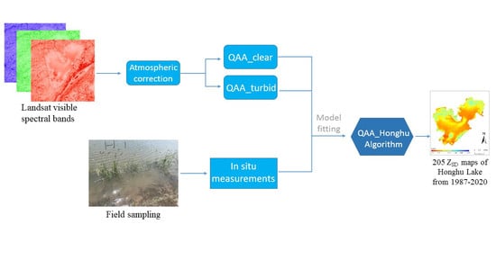
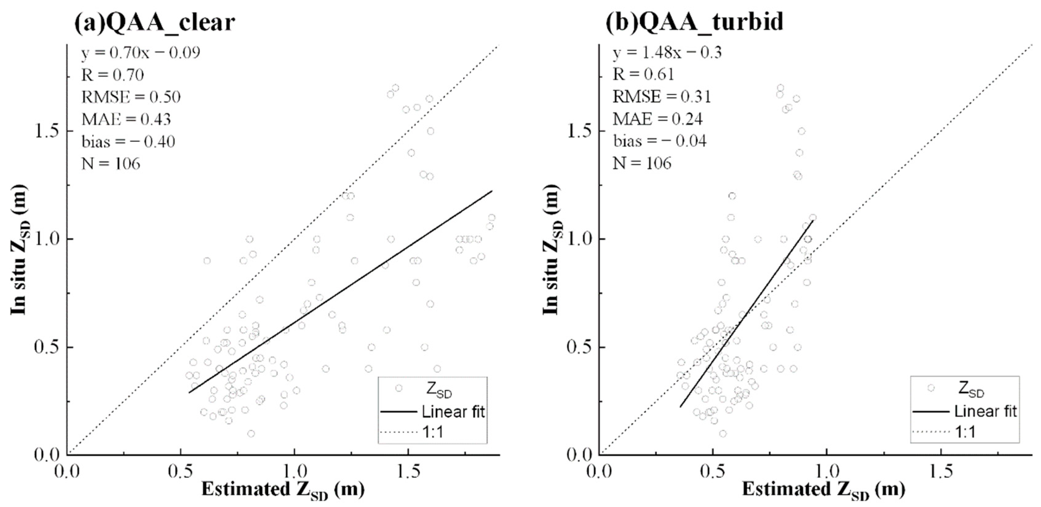
3.2. Developing a Combined Model for Honghu Lake

We found that QAA_v6 identified all of the water bodies in Honghu Lake as turbid water, which meant that only QAA_turbid could be applied. Then, we used QAA_turbid and QAA_clear separately, and the results showed that QAA_turbid severely underestimated the ZSD, while QAA_clear overestimated it. Moreover, water bodies of inland lakes usually change continuously between the two states of clear and turbid water. This change is rapid and a burst of wind and waves can cause relatively clear water to become very turbid. We assumed that QAA_clear and QAA_turbid change uniformly with the two states, rather than being switched by a threshold value. We proposed a combined model that simulated the transition of QAA_turbid to QAA_clear according to the uniform change process of the ZSD.
According to the characteristics of this process, we used logistic regression, a binary logistic model, to fit the model. The logistic model has been commonly used for binary regression, and it is frequently used in many areas, such as biology, economics, etc. [35]. There are three stages in our hypothesis: when the ZSD is very low, the proportion of QAA_clear is 0; when the ZSD is high enough, the coefficient of QAA_clear is 1; in another case, each of the two models has a certain proportion. The coefficient of QAA_clear and QAA_turbid varies continuously between 0 and 1. For this type of modeling, logistic regression is very suitable. We labeled the case where the water was turbid as 0, and the case where water was clear as 1. The regression was fitted with the lsqcurvefit function in MATLAB. The model (Figure 2) returned the weights of these two cases. We used the coefficient of QAA_clear to build a logistic function. It can be expressed as follows:
C c l e a r = 1 / ( 1 + e k × ( Z S D c l e a r x 0 ) )
where C c l e a r and Z S D c l e a r are the proportion and the ZSD estimation of QAA_clear. k and x0 are the steepness and the x value of the midpoint of the curve, and the sum of the proportion of QAA_turbid and QAA_clear should be 1.
Figure 2 illustrates the variation process of coefficients of the models. To fit this logistic curve, we chose the least-squares method. The basis of this method is to approximate the model and refine the parameters through successive iterations. There were 106 match-ups used for the fitting process. The values of QAA_clear and QAA_turbid are calculated for each sample point to obtain Z S D c l e a r and Z S D t u r b i d . These two model values and the in situ-measured data were put into the logistic model to fit the model parameters of Equation (3). After fitting the coefficients of the two models, the ZSD was therefore calculated as:
Z S D = C c l e a r × Z S D c l e a r + C t u r b i d × Z S D t u r b i d
where C c l e a r and C c l e a r are the coefficients of QAA_clear and QAA_turbid. Z S D c l e a r and Z S D t u r b i d are the estimations of the two models.
After we fit the logistic model, we can derive the threshold Rrs (656) value from Equation (3) and Table 2. In Figure 2, we can find the approximate position of the thresholds (the dotted line). If the ZSD value is smaller than the first threshold, then QAA_turbid is used; if it is greater than the second threshold, then QAA_clear is applied; in the middle of the two threshold values, each of the two models has a certain proportion. In order to obtain the accurate threshold values, we used the change rate of the curve curvature. For the formula like Equation (3), its curvature is Equation (5):
K = | f ( x ) | ( 1 + f 2 ( x ) ) 3 / 2
f(x) is C c l e a r in Equation (3) with model parameters, and f ( x ) and f ( x ) are the first- and second-order derivatives of f(x), respectively. The two threshold values correspond to the maxima and minima of the derivative formula for the rate of change K. The two threshold Rrs (656) can thus be derived by inversing the corresponding ZSD values according to the equations in Table 2.

3.3. Applying QAA to Landsat TM and ETM+ Data

Landsat OLI/TIRS has acquired about 10,000 scenes since it was launched in 2013. To provide the long time-series water clarity monitoring, we used Landsat TM and ETM+ data. Landsat series satellites have a 30 m spatial resolution and are ideal for monitoring inland lakes. Landsat series data has been widely used in lake research [36,37,38], and some studies have validated the applicability of Landsat TM, ETM+ in QAA [16,17,39]. OLI has a narrower spectrum compared to TM and ETM+, and OLI adds a shorter-wavelength blue band (0.43–0.45 μm) [40]. Due to the similarity of band 1, we used band 2 to replace band 1 for the experiment when applying OLI data to QAA. Figure 3 shows very little difference before and after the replacement. This experiment inspired us to apply TM and ETM+ data to QAA. The flow of applying QAA to TM and ETM+ is roughly the same as OLI (Table 2). The difference is the band substitute and the representative wavelength. Table 3 displays the representative wavelength of these sensors.
Normally, the direct substitute of 443 nm by 481 nm in QAA may lead to some changes in the results to a certain extent. It affects the empirical formula that determines a ( λ 0 ) and K d ( λ ) . To evaluate the error, we used Landsat-7 and Landsat-8 with overlapping acquisition dates to compare the results before and after the replacement. If this substitute works for Landsat-7, then it applies to Landsat-5 because of their similarity. Due to the satellite orbit settings, the time difference between the Landsat-7 and Landsat-8 satellite data is 8 days (Table 4). The ZSD is calculated through the Kd(λ) that is retrieved from QAA. We derived the minKd(λ) (the minimum Kd(λ) in the visible domain) and the ZSD from these satellite data using QAA_v6.

3.4. Error Metics and Statistical Indicators

To assess the performance of our algorithm, we used the following model-evaluation metrics: Pearson’s R (R), Mean Absolute Error (MAE), Root-Mean-Squared Error (RMSE) and bias. R represents how well the estimation fits the measurements; MSE shows how close the fitted line is to the data points; RMSE measures the distribution of the residuals and bias is a measure of the difference between the predicted values and the measured values. They are calculated as:
R M S E = 1 N i = 1 N ( y i y i ^ ) 2
M A E = 1 N i = 1 N | y i y i ^ |
b i a s = 1 N i = 1 N ( y i y i ^ )
where N is number of samples, y i ^ is the estimator and y i is the matched in situ measurement.

4. Results

4.1. ZSD Estimation from Landsat Data by QAA_Honghu

Figure 4 shows the comparison of the two models using 125 pairs of match-ups. QAA_clear had a result with slope = 0.70, R = 0.70, RMSE = 0.50, MAE = 0.43 and bias = −0.40 m. QAA_turbid had a result with slope = 1.48, R = 0.61, RMSE = 0.31, MAE = 0.24 and bias = −0.04. The slope of these two models illustrated that QAA_clear had an overestimate and QAA_turbid had an underestimate. Although the R of QAA_clear was relatively low, the other metrics of QAA_clear were very high, and Figure 4a shows that basically, all of the ZSD estimations of QAA_clear were higher than the in situ measurements. For QAA_turbid, on the other hand, most of its points were concentrated in the low-value region, and the higher the measured values, the more the ZSD estimations were underestimated. Therefore, the combined model is required in order to adopt the advantages of QAA_clear and QAA_turbid to improve the algorithm.
To develop this model, we used 106 matching pairs of field measurements and spectra-estimated ZSD in Honghu Lake from 2013 to 2020. We excluded sampling sites close to the lake shore because the bottom reflectance affects the water surface reflectance of shallow water areas [41,42,43]. The other parts of the match-ups were then used in the next section to validate QAA_Honghu. Then, we used these match-ups to fit the combined model coefficients according to Equation (4). It returned two model parameters: k = 11.84 and x0 = 0.99 (Figure 5). k is the steepness of the S-curve, and it controls the rate of curve growth [44]. The logistic curve is steepest at the midpoint, x0.
The parameters are applied to Equations (3) and (4). The ZSD calculations were:
Z S D = Z S D c l e a r 1 + e x p ( 11.84 × ( x 0.99 ) ) + Z S D t u r b i d × e x p ( 11.84 × ( x 0.99 ) ) 1 + e x p ( 11.84 × ( x 0.99 ) )
With certain model coefficients, we derived the Z S D c l e a r values of the threshold point, 0.67 m and 1.31 m. Next, we obtained the corresponding Rrs (656): if Rrs (656) < 0.010 sr−1, then the water will be determined as clear water; if Rrs (656) > 0.020 sr−1, then QAA_turbid will be applied. If Rrs (656) is between these two values, then both models will account for a certain proportion.
Figure 6 shows that QAA_Honghu had a significant improvement. Compared with QAA_clear and QAA_turbid, our model performed better with an RMSE that reduced from 0.5 to 0.28, an MAE that reduced from 0.43 to 0.21, and a bias that reduced from −0.4 to −0.05. Additionally, the trendline was closer to the 1:1 line. It improved the problem of too much deviation from the ZSD measurements.
We applied QAA_Honghu to Landsat TM, ETM+, and OLI imagery and obtained 205 ZSD maps with high spatial resolution. For these Landsat-7 data, we used the natural neighbor interpolation to fill the data gap. Figure 7 compared the trends between the measured ZSD and estimated ZSD from lake-centered sampling point Hu30 (29.829°N, 113.310°E). We used the average value within the 3 × 3 windows as the ZSD estimation. The results showed an overall consistency and the feasibility of QAA_Honghu for monitoring the process of changing water clarity. Figure 8 displays the ZSD of the Hu30 variation from 1987–2020, with an overall decreasing trend. Before 2000, the ZSD fluctuated significantly but quickly returned to peak value. Since then, although the fluctuation range of the ZSD was slight, the extreme values could not reach the previous level. There was a distinct downward trend from 2016–2020, and the peak values became smaller and smaller.
The ZSD of Honghu Lake showed a distinct seasonal pattern. Figure 9 demonstrates the ZSD variation from 1987–2020 by season; the ZSD in summer had the most evident downward trend, while the other seasons have also declined, but not to a great extent. Figure 10 shows the spatial distribution of the seasonal ZSD in 1991, 2016, and 2020. Overall, the ZSD was the highest in summer and the lowest in winter.

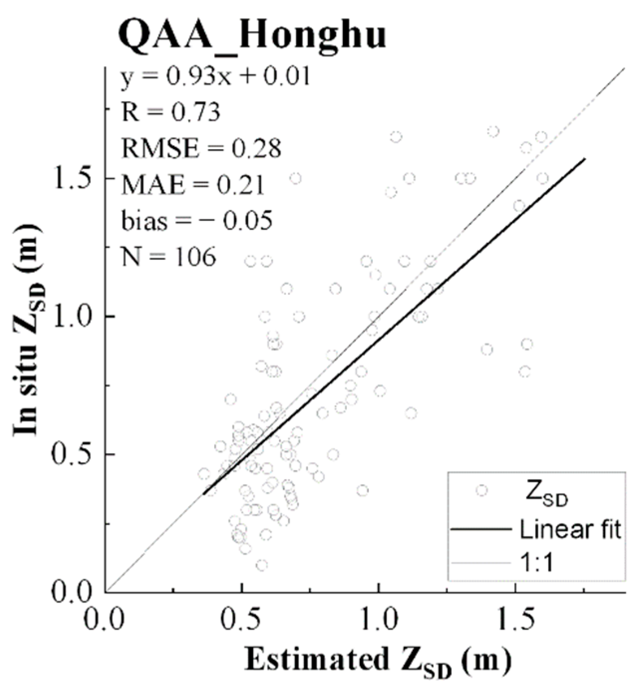
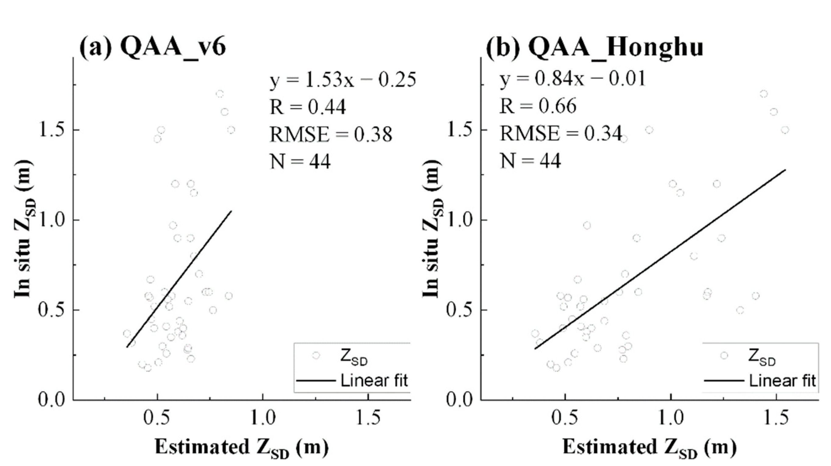
4.2. Validation of QAA_Honghu Using in Situ Measurements

We used 44 pairs of match-ups of Honghu Lake from 2013–2020 to verify the stability of this model. Compared to QAA_v6, QAA_Honghu had a more stable and better result with R = 0.66, RMSE = 0.34 and a slope closer to 1. A comparison of the ZSD estimations of QAA_v6 and QAA_Honghu (Figure 11) demonstrated the applicability of our model.

5. Discussion

5.1. The Performance of QAA_Honghu

Since the reference band and the threshold value set by the original algorithm (Rrs (656) = 0.0015 sr−1) did not apply to Honghu Lake, it caused the original QAA to identify all water as turbid water and seriously underestimated the ZSD. Instead of setting specific thresholds, our study fitted the respective percentage of QAA_clear and QAA_turbid by a logistic model. The critical values for QAA_clear and QAA_turbid corresponding to our fitted model were Rrs (656) = 0.010 sr−1 and Rrs (656) = 0.020 sr−1. When Rrs < 0.010 sr−1, QAA_clear is used; when Rrs > 0.020 sr−1, QAA_turbid is used; in addition to these two cases, each of the two models takes a certain percentage. We developed this combined model without a determination condition, which greatly improved the applicability of QAA in inland lakes. By fitting the coefficients of the two models, we obtained results with higher accuracy. Compared to the original algorithm, QAA_Honghu had a significant improvement in the validation dataset. QAA_Honghu had a higher R of 0.66, and the slope was closer to one. Moreover, this study improved the temporal resolution of the ZSD products by using Landsat-5,7,8 satellite data and covered 33 years of available data.

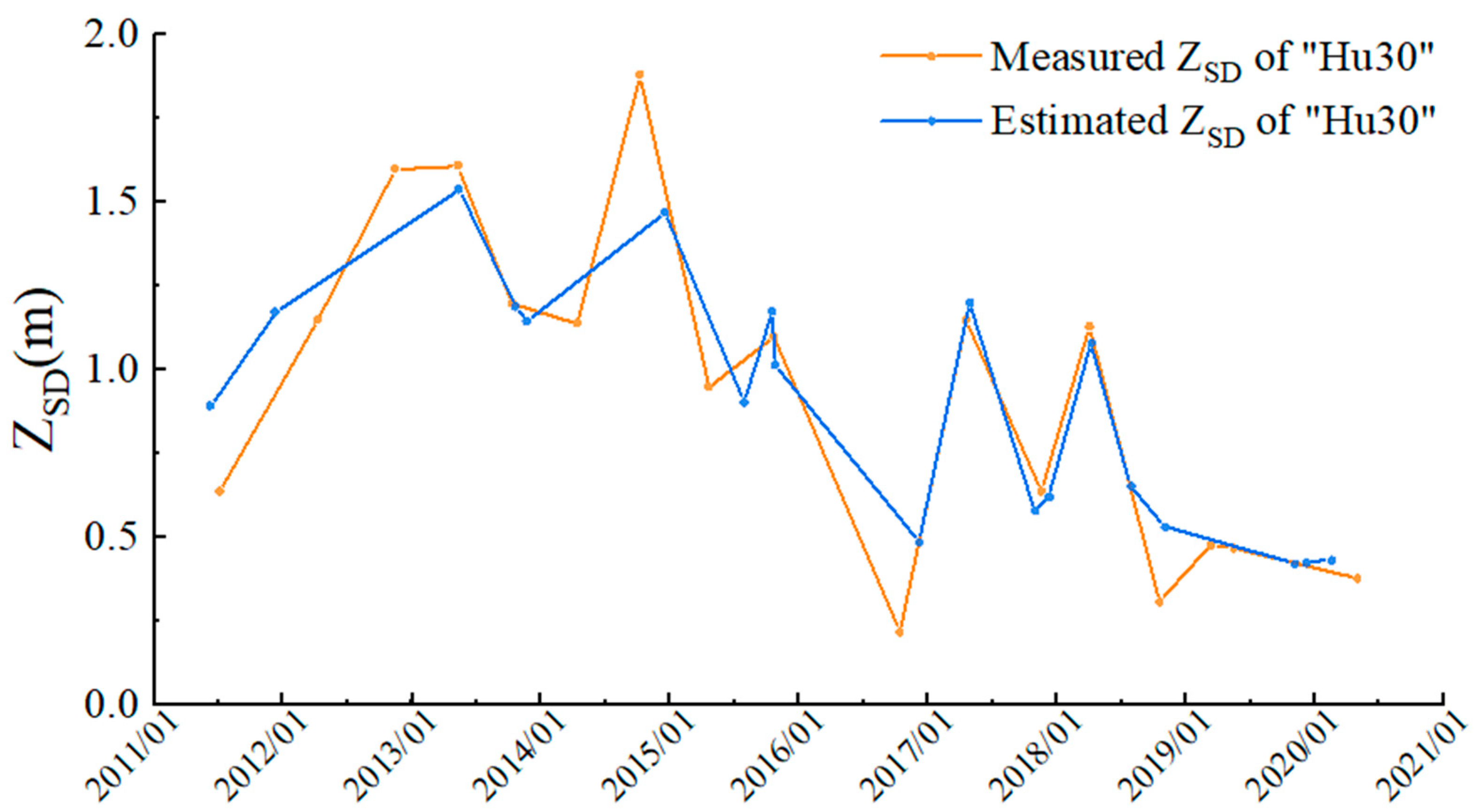
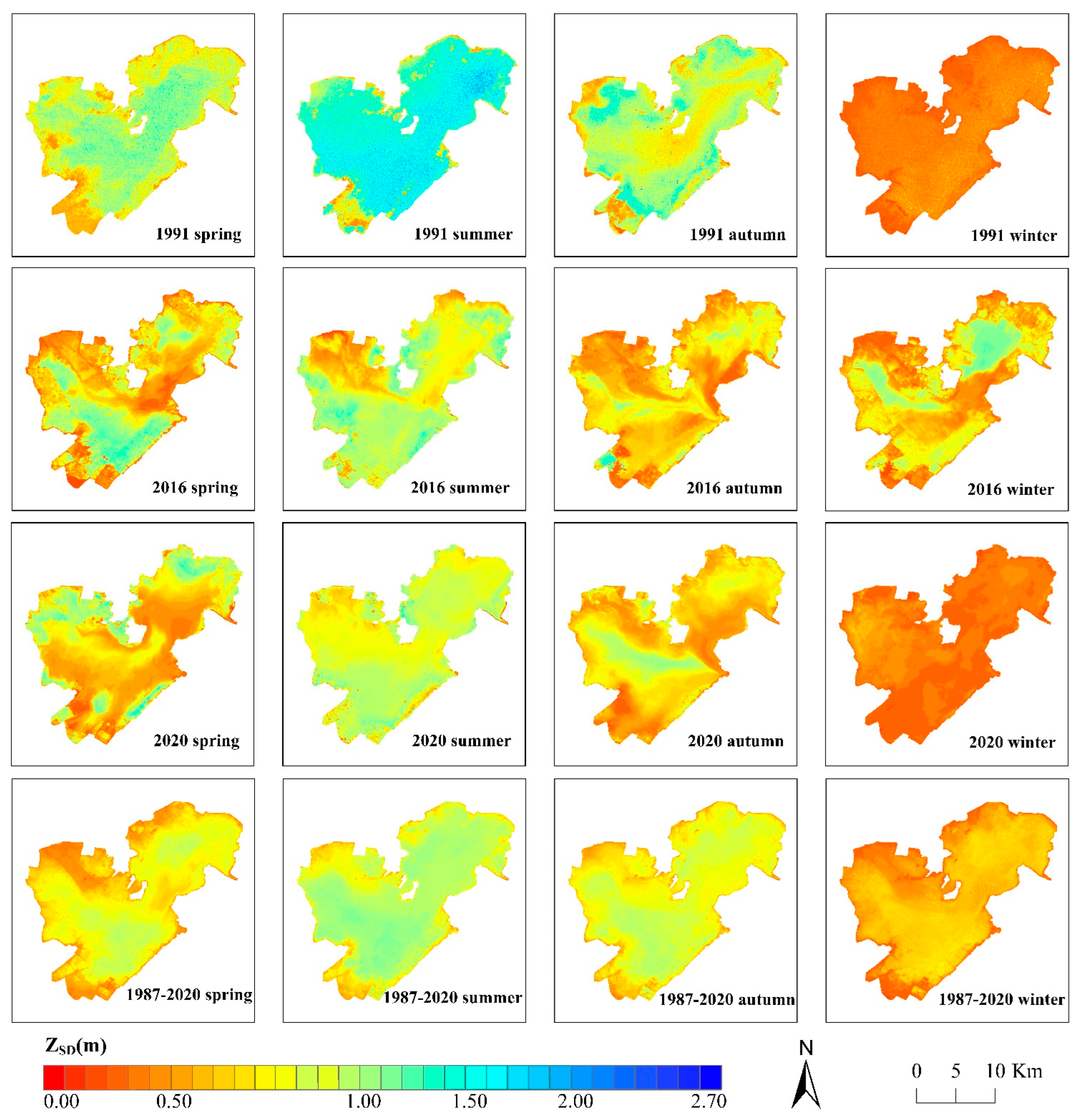
5.2. ZSD Trend of Honghu Lake

According to Figure 8, the ZSD showed an overall decreasing trend from 1987–2020. Before 2000, the ZSD fluctuated significantly, and the trendline was almost horizontal during this period. While some factors can significantly reduce the ZSD, Honghu Lake can recover, and it does so very quickly. From 2000–2016, the ZSD experienced a decline followed by an increase, and the peak values of the ZSD had difficulty reaching the previous values. The changes in the ZSD from 2000–2016 were primarily caused by human activities, especially enclosure aquaculture. Local fishermen used nets and bamboo poles to zone the open waters of Honghu Lake and then conducted aquaculture activities. Enclosure aquaculture remained an important factor in the ecological damage of Honghu Lake for a very long time [45,46,47]. After 2000, the area of enclosure aquaculture expanded rapidly. In 2004, the area reached 70% of the total lake area. During this period, the ZSD decreased rapidly. In 2005, the Hubei provincial government required the removal of the purse seine from Honghu Lake; the two largest ones were in 2005–2006 and 2013–2014. Since these two large-scale seine removals, the ZSD of Honghu Lake has increased. By 2017, the purse seine was completely removed.
In addition to human activities, extreme climatic events can also affect the water clarity of Honghu Lake. We found that the ZSD of Honghu Lake decreased after floods. The ZSD decreased to extreme values for some time immediately after the floods of 1996 and 1998 but quickly recovered to high levels. Then, after the catastrophic flood in 2016, the ZSD continued declining until 2020. It was mentioned above that all of the purse seines were removed around 2017, yet the water clarity of Honghu Lake did not rise as expected.
Some studies showed that the catastrophic flood in 2016 led to the extensive death of aquatic vegetation in Honghu Lake, which decayed and deposited, further deteriorating the water quality of Honghu Lake [48]. Enclosure aquaculture can also lead to a reduction in the environmental carrying capacity, making it difficult to restore the ecological functions of Honghu Lake after flooding [49]. This flood has degraded the ecological system of Honghu Lake and made it difficult to restore water clarity to the previous level.
Overall, the ZSD had a distinct seasonal variation from 1987–2020, with the highest in summer and the lowest in winter, and some early research had consistent results [15,50,51]. The drivers of this seasonal variation were also well-described by Feng et al. (2019), and it was caused by the rapid seasonal change in wind speed and precipitation in the Yangtze Plain [15,50,52].

5.3. Future Implication

In our study, we found that the error of QAA may originate from many factors. Firstly, the substitute of 443 nm by 481 nm had some impact. We used Landsat-7 and Landsat-8 data with overlapping acquisition dates (Table 4) to compare the satellite retrievals before and after the replacement. We generated 21 random points evenly over the study area and calculated the average value of minKd(λ) and ZSD from the satellite data. Average values can reduce the effect of the eight-day time window. Figure 12 shows the difference between the retrievals from Landsat-7 and Landsat-8. The minKd(λ) values (Figure 12a) from Landsat-7 of most of these 21 points were smaller than the results from Landsat-8. The bias between minKd(λ) from Landsat-7 and Landsat-8 was −0.018. Since the ZSD is inversely proportional to Kd(λ), most of the ZSD estimations (Figure 12b) from Landsat-7 were greater than Landsat-8 with bias = 0.009. The substitute of 443 nm by 481 nm resulted in a mild overestimation of ZSD. As a result, the relationship between Rrs (443) and Rrs (481) may change with the water optical properties and thus inevitably impact the results. Therefore, the above substitute is a kind of stopgap. Many studies have used empirical formulas or virtual-band estimators to solve the problem of missing bands [17,32]. These methods require a large amount of in situ-measured Rrs (λ) data, and we are also collecting such measured data to improve our algorithm.
Other factors also cause errors, such as the atmospheric correction, lake bottom, and the time-matching of measurement data with satellite data. Atmospheric correction is vital for a remotely sensed observation of water color [53]. The effect of the atmosphere over water bodies on the radiance is significant because water is highly absorptive [54]. The atmosphere of inland waters is more optically heterogeneous, making atmospheric correction more difficult. We have tried several frequently used methods and found ACOLITE is the most effective. Atmospheric-correction methods specifically for inland lake waters are urgent for such research. We also found in our experiments that a main problem in applying QAA to inland lakes was that the lake bottom affected the reflectance of the water surface in places with shallow water depth, and it decreased the accuracy of the algorithm. There are some studies to attenuate or quantify the impact of bottom reflectance [55]. Another way to increase the accuracy of QAA could be eliminating the error of the lake bottom. Another source of error is that the previous measured data do not intentionally match the image acquisition dates. Waters tend to change rapidly in inland lakes compared to relatively stable offshore waters. A single gust of wind and waves can quickly disturb the sediment in the lake, causing a rapid change in water clarity. Therefore, more satellite transit matching data are vital for improvement.
In recent years, the government has proposed many conservation measures to restore the water quality of Honghu Lake and protect the ecosystem diversity of its wetlands. The measures include removing all the purse seines, returning the embankments to the lake, and controlling pollution sources. However, the results so far have failed to reach expectations. Due to the limitation of data acquisition, this study could not quantitatively analyze the influence of various factors on the water clarity of Honghu Lake. In future research, NDVI data, water-level data, various meteorological data, and other water-quality parameters could be used to reveal the degree of influence factors.

6. Conclusions

The original QAA switches between QAA_clear and QAA_turbid by Rrs (656) = 0.0015 sr−1. It is unapplicable for inland lakes such as Honghu Lake. It caused the identification of all water bodies as turbid water. A new hypothesis in this research is that QAA_turbid and QAA_clear transition evenly. We developed a model for this change process. This model combines QAA_turbid and QAA_Honghu. After the modeling and validation, QAA_Honghu was applied to Landsat TM, Landsat ETM+, and Landsat OLI data for a total of 205 satellite imageries. The improved algorithm results reduced the RMSE from 0.5 to 0.28, the MAE from 0.43 to 0.21, and the bias from −0.4 to −0.05. The ZSD products with a high spatial resolution of Honghu Lake for 1987–2020 were obtained. Overall, the water clarity of Honghu Lake trended downward and demonstrated distinct seasonality.

Author Contributions

Conceptualization, M.C. and F.X.; methodology, M.C. and F.X.; software, M.C. and F.X.; validation, M.C. and Z.W.; formal analysis, M.C. and Q.F.; investigation, M.C., Q.F. and Y.Z.; resources, M.C., Z.W. and X.B.; data curation, M.C., Z.W. and Z.H.; writing—original draft preparation, M.C. and F.X.; writing—review and editing, M.C., F.X., Z.W., Q.F., X.B., Y.Z. and Z.H.; visualization, M.C.; supervision, F.X., Z.W., Q.F. and X.B.; project administration, F.X.; funding acquisition, F.X. All authors have read and agreed to the published version of the manuscript.

Funding

This research was funded by the Strategic Priority Research Program of the Chinese Academy of Sciences, (XDA23040201) and Key R & D projects in Hubei Province, (2020BCA074).

Data Availability Statement

Not applicable.

Acknowledgments

We thank the U.S. Geological Survey (USGS, https://www.usgs.gov/, accessed on 28 January 2021) for providing the Landsat data.

Conflicts of Interest

The authors declare no conflict of interest.

References

  1. Liu, X.; Zhang, Y.; Yin, Y.; Wang, M.; Qin, B. Wind and submerged aquatic vegetation influence bio-optical properties in large shallow Lake Taihu, China. J. Geophys. Res. Biogeosciences 2013, 118, 713–727. [Google Scholar] [CrossRef]
  2. Boyce, D.G.; Lewis, M.; Worm, B. Integrating global chlorophyll data from 1890 to 2010. Limnol. Oceanogr. Methods 2012, 10, 840–852. [Google Scholar] [CrossRef]
  3. Chen, Z.; Muller-Karger, F.E.; Hu, C. Remote sensing of water clarity in Tampa Bay. Remote Sens. Environ. 2007, 109, 249–259. [Google Scholar] [CrossRef]
  4. McCullough, I.M.; Loftin, C.S.; Sader, S.A. Combining lake and watershed characteristics with Landsat TM data for remote estimation of regional lake clarity. Remote Sens. Environ. 2012, 123, 109–115. [Google Scholar] [CrossRef]
  5. Majozi, N.P.; Salama, M.S.; Bernard, S.; Harper, D.M.; Habte, M.G. Remote sensing of euphotic depth in shallow tropical inland waters of Lake Naivasha using MERIS data. Remote Sens. Environ. 2014, 148, 178–189. [Google Scholar] [CrossRef]
  6. Deutsch, E.S.; Cardille, J.A.; Koll-Egyed, T.; Fortin, M.-J. Landsat 8 Lake Water Clarity Empirical Algorithms: Large-Scale Calibration and Validation Using Government and Citizen Science Data from across Canada. Remote Sens. 2021, 13, 1257. [Google Scholar] [CrossRef]
  7. Cao, Z.; Ma, R.; Duan, H.; Pahlevan, N.; Melack, J.; Shen, M.; Xue, K. A machine learning approach to estimate chlorophyll-a from Landsat-8 measurements in inland lakes. Remote Sens. Environ. 2020, 248, 111974. [Google Scholar] [CrossRef]
  8. Lee, Z.; Carder, K.L.; Arnone, R.A. Deriving inherent optical properties from water color: A multiband quasi-analytical algorithm for optically deep waters. Appl. Opt. 2002, 41, 5755–5772. [Google Scholar] [CrossRef]
  9. Pan, H.; Lyu, H.; Wang, Y.; Jin, Q.; Wang, Q.; Li, Y.; Fu, Q. An Improved Approach to Retrieve IOPs Based on a Quasi-Analytical Algorithm (QAA) for Turbid Eutrophic Inland Water. IEEE J. Sel. Top. Appl. Earth Obs. Remote Sens. 2015, 8, 5177–5189. [Google Scholar] [CrossRef]
  10. Ogashawara, I.; Mishra, D.R.; Nascimento, R.F.F.; Alcântara, E.H.; Kampel, M.; Stech, J.L. Re-parameterization of a quasi-analytical algorithm for colored dissolved organic matter dominant inland waters. Int. J. Appl. Earth Obs. Geoinf. 2016, 53, 128–145. [Google Scholar] [CrossRef] [Green Version]
  11. Hoge, F.E.; Lyon, P.E. Satellite retrieval of inherent optical properties by linear matrix inversion of oceanic radiance models: An analysis of model and radiance measurement errors. J. Geophys. Res. 1996, 101, 16631–16648. [Google Scholar] [CrossRef]
  12. Bukata, R.P.; Jerome, J.H.; Kondratyev, K.Y.; Pozdnyakov, D.V. Optical Properties and Remote Sensing of Inland and Coastal Waters; CRC Press: Boca Raton, FL, USA, 1995. [Google Scholar]
  13. Lee, Z.; Shang, S.; Hu, C.; Du, K.; Weidemann, A.; Hou, W.; Lin, J.; Lin, G. Secchi disk depth: A new theory and mechanistic model for underwater visibility. Remote Sens. Environ. 2015, 169, 139–149. [Google Scholar] [CrossRef] [Green Version]
  14. Chen, S.; Zhang, T. Evaluation of a QAA-based algorithm using MODIS land bands data for retrieval of IOPs in the Eastern China Seas. Opt. Express 2015, 23, 13953–13971. [Google Scholar] [CrossRef] [PubMed]
  15. Feng, L.; Hou, X.; Zheng, Y. Monitoring and understanding the water transparency changes of fifty large lakes on the Yangtze Plain based on long-term MODIS observations. Remote Sens. Environ. 2019, 221, 675–686. [Google Scholar] [CrossRef]
  16. Pitarch, J.; Bellacicco, M.; Organelli, E.; Volpe, G.; Colella, S.; Vellucci, V.; Marullo, S. Retrieval of Particulate Backscattering Using Field and Satellite Radiometry: Assessment of the QAA Algorithm. Remote Sens. 2019, 12, 77. [Google Scholar] [CrossRef] [Green Version]
  17. Yin, Z.; Li, J.; Liu, Y.; Xie, Y.; Zhang, F.; Wang, S.; Sun, X.; Zhang, B. Water clarity changes in Lake Taihu over 36 years based on Landsat TM and OLI observations. Int. J. Appl. Earth Obs. Geoinf. 2021, 102, 102457. [Google Scholar] [CrossRef]
  18. Cheng Feng, L.; Yun Mei, L.; Yong, Z.; Deyong, S.; Bin, Y. Validation of a Quasi-Analytical Algorithm for Highly Turbid Eutrophic Water of Meiliang Bay in Taihu Lake, China. IEEE Trans. Geosci. Remote Sens. 2009, 47, 2492–2500. [Google Scholar] [CrossRef]
  19. Yang, W.; Matsushita, B.; Chen, J.; Yoshimura, K.; Fukushima, T. Retrieval of Inherent Optical Properties for Turbid Inland Waters From Remote-Sensing Reflectance. IEEE Trans. Geosci. Remote Sens. 2013, 51, 3761–3773. [Google Scholar] [CrossRef]
  20. Mishra, S.; Mishra, D.R.; Lee, Z. Bio-Optical Inversion in Highly Turbid and Cyanobacteria-Dominated Waters. IEEE Trans. Geosci. Remote Sens. 2014, 52, 375–388. [Google Scholar] [CrossRef]
  21. Watanabe, F.; Mishra, D.R.; Astuti, I.; Rodrigues, T.; Alcântara, E.; Imai, N.N.; Barbosa, C. Parametrization and calibration of a quasi-analytical algorithm for tropical eutrophic waters. ISPRS J. Photogramm. Remote Sens. 2016, 121, 28–47. [Google Scholar] [CrossRef] [Green Version]
  22. Wang, Y.; Shen, F.; Sokoletsky, L.; Sun, X. Validation and Calibration of QAA Algorithm for CDOM Absorption Retrieval in the Changjiang (Yangtze) Estuarine and Coastal Waters. Remote Sens. 2017, 9, 1192. [Google Scholar] [CrossRef] [Green Version]
  23. Jiang, D.; Matsushita, B.; Setiawan, F.; Vundo, A. An improved algorithm for estimating the Secchi disk depth from remote sensing data based on the new underwater visibility theory. ISPRS J. Photogramm. Remote Sens. 2019, 152, 13–23. [Google Scholar] [CrossRef]
  24. Liu, X.; Lee, Z.; Zhang, Y.; Lin, J.; Shi, K.; Zhou, Y.; Qin, B.; Sun, Z. Remote Sensing of Secchi Depth in Highly Turbid Lake Waters and Its Application with MERIS Data. Remote Sens. 2019, 11, 2226. [Google Scholar] [CrossRef] [Green Version]
  25. Zeng, S.; Lei, S.H.; Li, Y.M.; Lyu, H.; Xu, J.F.; Dong, X.Z.; Wang, R.; Yang, Z.Q.; Li, J.C. Retrieval of Secchi Disk Depth in Turbid Lakes from GOCI Based on a New Semi-Analytical Algorithm. Remote Sens. 2020, 12, 1516. [Google Scholar] [CrossRef]
  26. Somasundaram, D.; Zhang, F.; Ediriweera, S.; Wang, S.; Yin, Z.; Li, J.; Zhang, B. Patterns, Trends and Drivers of Water Transparency in Sri Lanka Using Landsat 8 Observations and Google Earth Engine. Remote Sens. 2021, 13, 2193. [Google Scholar] [CrossRef]
  27. Li, S.; Song, K.; Mu, G.; Zhao, Y.; Ma, J.; Ren, J. Evaluation of the Quasi-Analytical Algorithm (QAA) for Estimating Total Absorption Coefficient of Turbid Inland Waters in Northeast China. IEEE J. Sel. Top. Appl. Earth Obs. Remote Sens. 2016, 9, 4022–4036. [Google Scholar] [CrossRef]
  28. Najah, A.; Al-Shehhi, M.R. Performance of the Ocean Color Algorithms: QAA, GSM, and GIOP in Inland and Coastal Waters. Remote Sens. Earth Syst. Sci. 2021, 4, 235–248. [Google Scholar] [CrossRef]
  29. Shang, S.; Dong, Q.; Lee, Z.; Li, Y.; Xie, Y.; Behrenfeld, M. MODIS observed phytoplankton dynamics in the Taiwan Strait: An absorption-based analysis. Biogeosciences 2011, 8, 841–850. [Google Scholar] [CrossRef] [Green Version]
  30. Chen, J.; He, X.; Liu, Z.; Lin, N.; Xing, Q.; Pan, D. Sun glint correction with an inherent optical properties data processing system. Int. J. Remote Sens. 2021, 42, 617–638. [Google Scholar] [CrossRef]
  31. Warren, M.A.; Simis, S.G.H.; Selmes, N. Complementary water quality observations from high and medium resolution Sentinel sensors by aligning chlorophyll-a and turbidity algorithms. Remote Sens. Environ. 2021, 265, 112651. [Google Scholar] [CrossRef] [PubMed]
  32. Lee, Z.; Shang, S.; Qi, L.; Yan, J.; Lin, G. A semi-analytical scheme to estimate Secchi-disk depth from Landsat-8 measurements. Remote Sens. Environ. 2016, 177, 101–106. [Google Scholar] [CrossRef]
  33. Vanhellemont, Q. Adaptation of the dark spectrum fitting atmospheric correction for aquatic applications of the Landsat and Sentinel-2 archives. Remote Sens. Environ. 2019, 225, 175–192. [Google Scholar] [CrossRef]
  34. Vanhellemont, Q.; Ruddick, K. Atmospheric correction of metre-scale optical satellite data for inland and coastal water applications. Remote Sens. Environ. 2018, 216, 586–597. [Google Scholar] [CrossRef]
  35. Jukić, D.; Scitovski, R. Solution of the least-squares problem for logistic function. J. Comput. Appl. Math. 2003, 156, 159–177. [Google Scholar] [CrossRef] [Green Version]
  36. Carpenter, D.J.; Carpenter, S.M. Modeling inland water quality using Landsat data. Remote Sens. Environ. 1983, 13, 345–352. [Google Scholar] [CrossRef]
  37. Kloiber, S.M.; Brezonik, P.L.; Bauer, M.E. Application of Landsat imagery to regional-scale assessments of lake clarity. Water Res. 2002, 36, 4330–4340. [Google Scholar] [CrossRef]
  38. Song, K.; Liu, G.; Wang, Q.; Wen, Z.; Lyu, L.; Du, Y.; Sha, L.; Chong, F. Quantification of lake clarity in China using Landsat OLI imagery data. Remote Sens. Environ. 2020, 243, 111800. [Google Scholar] [CrossRef]
  39. Zhang, Y.; Zhang, Y.; Shi, K.; Zhou, Y.; Li, N. Remote sensing estimation of water clarity for various lakes in China. Water Res. 2021, 192, 116844. [Google Scholar] [CrossRef]
  40. Roy, D.P.; Kovalskyy, V.; Zhang, H.K.; Vermote, E.F.; Yan, L.; Kumar, S.S.; Egorov, A. Characterization of Landsat-7 to Landsat-8 reflective wavelength and normalized difference vegetation index continuity. Remote Sens. Environ. 2016, 185, 57–70. [Google Scholar] [CrossRef] [Green Version]
  41. Ackleson, S.G. Diffuse attenuation in optically-shallow water: Effects of bottom reflectance. Ocean. Opt. XIII 1997, 2963, 326–330. [Google Scholar]
  42. Islam, A.; Gao, J.; Ahmad, W.; Neil, D.; Bell, P. A composite DOP approach to excluding bottom reflectance in mapping water parameters of shallow coastal zones from TM imagery. Remote Sens. Environ. 2004, 92, 40–51. [Google Scholar] [CrossRef]
  43. Yu, Y.; Chen, S.; Qin, W.; Lu, T.; Li, J.; Cao, Y. A Semi-Empirical Chlorophyll-a Retrieval Algorithm Considering the Effects of Sun Glint, Bottom Reflectance, and Non-Algal Particles in the Optically Shallow Water Zones of Sanya Bay Using SPOT6 Data. Remote Sens. 2020, 12, 2765. [Google Scholar] [CrossRef]
  44. Choudhary, R.; Gianey, H.K. Comprehensive review on supervised machine learning algorithms. In Proceedings of the 2017 International Conference on Machine Learning and Data Science (MLDS), Noida, India, 14–15 December 2017; pp. 37–43. [Google Scholar]
  45. Ban, X.; Yu, C.; WeiI, K.; Du, Y. Analysis of Influence of Enclosure Aquaculture on Water Quality of Honghu Lake. Environ. Sci. Technol. 2010, 33, 125–129. [Google Scholar]
  46. Jiang, L.; Wang, X.; EnHua, L.; Cai, X.; Deng, F. Water Quality Change Characteristics and Driving Factors of Honghu Lake before and after Ecological Restoration. Wetl. Sci. 2012, 10, 188–193. [Google Scholar]
  47. Yu, H.; Wang, H.; Wand, H.; Liang, Y.; Li, X. Lake Demolition Monitoring and Estimation of Ecological Environment Benefits in Jianghan Plain: A Case Study of the Honghu Lake. Resour. Environ. Yangtze Basin 2020, 29, 2760–2769. [Google Scholar]
  48. LI, E.; Yang, C.; Cai, X.; Wang, Z.; Wang, X. Plant Diversity and Protection Measures in Honghu Wetland. Resour. Environ. Yangtze Basin 2021, 30, 623–635. [Google Scholar]
  49. Liu, K.; Zhou, S.; Huang, Y.; Tang, Y.; Li, R. The Impact of Land Use Changes on Flood Disaster in the Honghu Lake Watershed. Adv. Meteorol. Sci. Technol. 2018, 8, 63–66. [Google Scholar]
  50. Shi, K.; Zhang, Y.; Zhu, G.; Liu, X.; Zhou, Y.; Xu, H.; Qin, B.; Liu, G.; Li, Y. Long-term remote monitoring of total suspended matter concentration in Lake Taihu using 250 m MODIS-Aqua data. Remote Sens. Environ. 2015, 164, 43–56. [Google Scholar] [CrossRef]
  51. Hou, X.; Feng, L.; Duan, H.; Chen, X.; Sun, D.; Shi, K. Fifteen-year monitoring of the turbidity dynamics in large lakes and reservoirs in the middle and lower basin of the Yangtze River. Remote Sens. Environ. 2017, 190, 107–121. [Google Scholar] [CrossRef]
  52. Hu, C.; Lee, Z.; Ma, R.; Yu, K.; Li, D.; Shang, S. Moderate resolution imaging spectroradiometer (MODIS) observations of cyanobacteria blooms in Taihu Lake. J. Geophys. Res. Ocean. 2010, 115. [Google Scholar] [CrossRef] [Green Version]
  53. Liu, G.; Li, Y.; Lyu, H.; Wang, S.; Du, C.; Huang, C. An improved land target-based atmospheric correction method for Lake Taihu. IEEE J. Sel. Top. Appl. Earth Obs. Remote Sens. 2015, 9, 793–803. [Google Scholar] [CrossRef]
  54. Moses, W.J.; Sterckx, S.; Montes, M.J.; De Keukelaere, L.; Knaeps, E. Atmospheric correction for inland waters. In Bio-Optical Modeling and Remote Sensing of Inland Waters; Elsevier: Amsterdam, The Netherlands, 2017; pp. 69–100. [Google Scholar] [CrossRef]
  55. Ma, Y.; Zhang, H.; Li, X.; Wang, J.; Cao, W.; Li, D.; Lou, X.; Fan, K. An Exponential Algorithm for Bottom Reflectance Retrieval in Clear Optically Shallow Waters from Multispectral Imagery without Ground Data. Remote Sens. 2021, 13, 1169. [Google Scholar] [CrossRef]
Figure 1. Map of Honghu Lake with 24 in situ sampling sites. It is located in the middle reaches of the Yangtze River.
Remotesensing 14 03798 g001
Figure 2. Logistic equation of coefficients of QAA_clear. The vertical dashed line represents the threshold value for switching models. The curve has three stages of change: the first only applies QAA_turbid, the second is when both models have contributions, and the third only uses QAA_clear.
Remotesensing 14 03798 g002
Figure 3. Scatter plots of before and after the replacement of the estimated ZSD of Landsat OLI data with a 1:1 fit line.
Remotesensing 14 03798 g003
Figure 4. Scatter plots of Landsat-estimated ZSD and in situ-measured ZSD for (a) QAA_clear and (b) QAA_turbid. The field data were gathered ±1–7 days of Landsat satellite overpass.
Remotesensing 14 03798 g004
Figure 5. Function diagram of coefficients of QAA_clear after bringing in the parameters.
Remotesensing 14 03798 g005
Figure 6. Scatter plots of Landsat-estimated ZSD and in situ-measured ZSD for QAA_Honghu. The field data were gathered ±1–7 days of Landsat satellite overpass.
Remotesensing 14 03798 g006
Figure 7. The Landsat-estimated ZSD and in situ-measured ZSD trend at sampling point Hu30.
Remotesensing 14 03798 g007
Figure 8. Time series of Landsat-estimated ZSD (mean value of the central lake area) from 1987–2020. There are 205 points in total, with a general downward trend.
Remotesensing 14 03798 g008
Figure 9. Time series of Landsat-estimated ZSD (mean value of the main area of Honghu Lake, the buffer zone generated 2 km inward from Honghu Lake boundary) by season from 1987–2020. The red lines are the trend lines of each season.
Remotesensing 14 03798 g009
Figure 10. Spatial distribution of seasonal ZSD retrieved from QAA_Honghu in 1991, 2016 and 2020 and the mean ZSD of 1987–2020. These 12 representative images were selected by season and acquired on 16 May 1991, 19 July 1991, 7 October 1991, 27 January 1992, 1 March 2016, 23 July 2016, 12 November 2016, 16 February 2017, 29 April 2020, 3 August 2020, 7 November 2020, and 25 December 2020.
Remotesensing 14 03798 g010
Figure 11. Comparison between in situ ZSD and estimated ZSD using (a) QAA_v6, (b) QAA_Honghu.
Remotesensing 14 03798 g011
Figure 12. Average ZSD (a) and minKd(λ) (b) plots of 21 sample points. The value of each dot is the average of retrievals from Landsat-7 and Landsat-8 in Table 4.
Remotesensing 14 03798 g012
Table 1. Image type and dates of image acquisition and in situ sampling.
Image Type Image DateSampling Date
Landsat-812 May 20139 May 2013
Landsat-711 October 20139 October 2013
Landsat-86 October 20147 October 2014
Landsat-825 October 201521 October 2015
Landsat-713 April 201717 April 2017
Landsat-88 April 1082 April 2018
Landsat-81 August 201926 July 2019
Landsat-85 November 201914 November 2019
Landsat-829 April 202029 April 2020
Table 2. Steps of QAA_v6 for Landsat OLI.
StepCalculation
1 r r s ( λ ) = R r s ( λ ) / ( 0.52 + 1.7 R r s ( λ ) )
2 u ( λ ) = g 0 + ( g 0 ) 2 + 4 g 1 × r r s ( λ ) 2 g 1 , where g 0 =0.089, g 1 =0.1245
3QAA_clear ( R r s ( 656 ) < 0.0015 s r 1 )QAA_turbid (Else)
4 χ = l o g ( r r s ( 443 ) + r r s ( 483 ) r r s ( 554 ) + 5 r r s ( 656 ) r r s ( 483 ) r r s ( 665 ) )
a ( λ 0 ) = a ( 554 ) = a w ( 554 ) + 10 h 0 + h 1 χ + h 2 χ 2 ,   where   h 0 = 1.146 ,   h 1 = 1.366 ,   and   h 2 = 0.469
a ( λ 0 ) = a ( 665 ) = a w ( 665 ) + 0.39 ( R r s ( 656 ) R r s ( 443 ) + R r s ( 483 ) ) 1.14
5 b b p ( λ 0 ) = b b p ( 554 ) = u ( 554 ) × a ( 554 ) 1 u ( 554 ) b b w ( 554 ) b b p ( λ 0 ) = b b p ( 656 ) = u ( 656 ) × a ( 656 ) 1 u ( 656 ) b b w ( 656 )
6 η = 2.0 ( 1 1.2 e x p ( 0.9 r r s ( 443 ) r r s ( 554 ) ) )
7 b b p ( λ ) = b b p ( λ 0 ) ( λ 0 λ ) η
8 a ( λ ) = ( 1 u ( λ ) ) ( b b w ( λ ) + b b p ( λ ) ) / u ( λ )
9 b b ( λ ) = u ( λ ) × a ( λ ) 1 u ( λ )
10 K d ( λ ) = ( 1 + 0.005 × θ s ) a ( λ ) + ( 1 0.265 b b w ( λ ) b b ( λ ) ) × 4.26 × ( 1 0.52 × e 10.8 × a ( λ ) ) b b ( λ )
Notes: r r s ( λ ) : below-surface remote sensing reflectance; R r s ( λ ) : above-surface remote sensing reflectance; u ( λ ) : ratio of backscattering coefficient to the sum of absorption and backscattering coefficients; λ 0 : a reference wavelength; a ( λ ) : absorption coefficient of the total; a w ( λ ) : absorption coefficient of pure water; b b p ( λ ) : backscattering coefficient of suspended particles; b b w ( λ ) : backscattering coefficient of pure seawater; η : spectral power for particle backscattering coefficient; K d ( λ ) : diffuse attenuation coefficient; θ s : the solar zenith angle.
Table 3. The representative wavelength of TM, ETM+ and OLI visible bands.
Band
Wavelength (nm)
TMETM+OLI
Band 1486479443
Band 2571561481
Band 3668661554
Band 4 656
Table 4. Images acquisition dates of Landsat-7 and Landsat-8.
Landsat-7 DateLandsat-8 Date
23 July 201331 July 2013
30 December 201322 December 2013
17 October 201525 October 2014
4 November 201612 November 2016
9 December 201717 December 2017
25 August 201917 August 2019
15 November 20207 November 2020
Publisher’s Note: MDPI stays neutral with regard to jurisdictional claims in published maps and institutional affiliations.

