Article

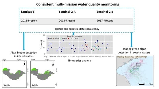
Evaluating Landsat-8 and Sentinel-2 Data Consistency for High Spatiotemporal Inland and Coastal Water Quality Monitoring

1
Department of Land Surveying and Geo-Informatics, The Hong Kong Polytechnic University, Kowloon, Hong Kong, China
2
Research Institute for Land and Space, The Hong Kong Polytechnic University, Kowloon, Hong Kong, China
3
Center for Geographic Information System, University of the Punjab, Lahore 54590, Pakistan
4
Remote Sensing, GIS and Climatic Research Lab (RSGCRL), National Center of GIS and Space Applications, University of the Punjab, Lahore 54590, Pakistan
5
Department of Physics and Technology, Earth Observation Division, The Arctic University of Norway, 9019 Tromsø, Norway
*
Author to whom correspondence should be addressed.
Remote Sens. 2022, 14(13), 3155; https://0-doi-org.brum.beds.ac.uk/10.3390/rs14133155
Submission received: 30 April 2022 / Revised: 22 June 2022 / Accepted: 27 June 2022 / Published: 30 June 2022
(This article belongs to the Special Issue Optical Remote Sensing for Surface Water Parameters Retrieval)

Abstract

:
The synergy of fine-to-moderate-resolutin (i.e., 10–60 m) satellite data of the Landsat-8 Operational Land Imager (OLI) and the Sentinel-2 Multispectral Instrument (MSI) provides a possibility to monitor the dynamics of sensitive aquatic systems. However, it is imperative to assess the spectral consistency of both sensors before developing new algorithms for their combined use. This study evaluates spectral consistency between OLI and MSI-A/B, mainly in terms of the top-of-atmosphere reflectance ( ρ t ) , Rayleigh-corrected reflectance ( ρ r c ) ,   and   remote-sensing reflectance ( R r s ) . To check the spectral consistency under various atmospheric and aquatic conditions, near-simultaneous same-day overpass images of OLI and MSI-A/B were selected over diverse coastal and inland areas across Mainland China and Hong Kong. The results showed that spectral data obtained from OLI and MSI-A/B were consistent. The difference in the mean absolute percentage error (MAPE) of the OLI and MSI-A products was ~8% in ρ t and ~10% in both ρ r c   and R r s for all the matching bands, whereas the MAPE for OLI and MSI-B was ~3.7% in ρ t , ~5.7% in ρ r c , and ~7.5%   in   R r s for all visible bands except the ultra-blue band. Overall, the green band was the most consistent, with the lowest MAPE of ≤ 4.6% in all the products. The linear regression model suggested that product difference decreased significantly after band adjustment with the highest reduction rate in R r s (NIR band) and R r s (red band) for the OLI–MSI-A and OLI–MSI-B comparison, respectively. Further, this study discussed the combined use of OLI and MSI-A/B data for (i) time series of the total suspended solid concentrations (TSS) over coastal and inland waters; (ii) floating algae area comparison; and (iii) tracking changes in coastal floating algae (FA). Time series analysis of the TSS showed that seasonal variation was well-captured by the combined use of sensors. The analysis of the floating algae bloom area revealed that the algae area was consistent, however, the difference increases as the time difference between the same-day overpasses increases. Furthermore, tracking changes in coastal FA over two months showed that thin algal slicks (width < 500 m) can be detected with an adequate spatial resolution of the OLI and the MSI.

Graphical Abstract

1. Introduction

Coastal and inland waters are adversely affected by the anthropogenic activities and climate change. Population density within 100 km of coastlines is three times higher than the average density of the global population [1]. Coastal cities rely on both a high-quality resource of drinking water and clean coastal resources for sustainable coastal ecosystems and coastal economy. Inland freshwater resources are also a vital source of drinking water, providers of ecosystem services, centers of recreational activities, and homes to aquatic species. Increasing land exploitation activities and changing climate are posing threats to coastal and inland waters [2]. Heavy nutrients flow into these water resources from land activities as changing agricultural practices and improper management of industrial waste have led to more frequent occurrences of harmful algae blooms that endanger human health, economy, and aquatic ecosystems [3,4,5].
To cope with the adverse consequences of water pollution, there is an urgent need to monitor the potential changes in these water resources [6,7]. The traditional methods adopted to monitor these resources are labor-intensive and time-consuming. Consistent coverage with high temporal resolution of ~2–3 days of the Landsat and Sentinel-2 (S-2 hereafter) virtual constellation along with an adequate spatial resolution from 10–30 m [8] provides possibilities for reliable monitoring of aquatic systems [9]. In the coming 10–15 years, the Multispectral Imager (MSI) onboard Sentinel-2 mission and the Operational Land Imager (OLI) onboard Landsat-8/9 are expected to provide well-calibrated and robust water quality products [10,11]. High-frequency revisits can be fully achieved as Landsat-9 also became operational in 2021. Considering the data gaps caused by cloud cover and various environmental conditions, this temporal frequency is critical in capturing dynamic coastal and inland waters. With reliable radiometric performances, the OLI and the MSI can monitor several water quality indicators, such as chlorophyll-a (Chl-a) [12], suspended particulate matter (SPM) or total suspended solids (TSS) [13,14,15], and water clarity [16]. Both the OLI and the MSI have four visible bands, i.e., ultra-blue/coastal aerosol, blue, green, and red. In addition to the four visible bands, the OLI has one near-infrared (NIR) band and two shortwave-infrared (SWIR) bands, while MSI has three additional NIR bands that allow the use of alternative algorithms for retrieving Chl-a or other pigments responsible for inland/coastal algae blooms [17,18,19]. This undoubtedly makes the MSI more effective in studying algae blooms and Chl-a. The MSI also has one NIR and two SWIR bands, similarly (i.e., closely spaced) to the OLI.
Recent studies have proved the efficiency of Landsat-8 (L-8) OLI and/or S-2 MSI data for the monitoring of coastal and inland resources. Vanhellemont and Ruddick [20] studied the impact of offshore wind farms on the TSS and quantified the width and length of plumes. OLI data with adequate spatial resolution were adopted to study dynamic thin turbid wakes. Qiu et al. [21] retrieved the TSS in the Yellow River estuary using OLI data. With the use of the MSI, Gernez et al. [22] studied the influence of Chl-a and TSS concentrations on oyster physiological responses in an economically important intertidal zone, and highlighted the importance of the MSI red and NIR bands for estimation of the TSS [23]. Liu et al. [13] highlighted the use of an additional NIR band (783 nm) of the MSI in the retrieval of the TSS in Poyang Lake. Hafeez and Wong [14] also studied small coastal algae blooms in turbid waters of Hong Kong using MSI data. Other similar studies have either demonstrated the use of MSI data for water quality [24] or algorithm development and bottom mapping [25]. The combined use of two sensors is important for high temporal monitoring. Many studies have demonstrated the use of harmonized OLI and MSI time-series data for diverse terrestrial applications, such as detection of irrigated areas [26], urban areas, evaluation of land indices [27], monitoring selective logging [28], winter crop mapping and winter wheat yield [29], and crop monitoring [30]. However, to our knowledge, there is limited work on aquatic applications using combined satellite sensor data. Only a few studies have explained the combined use of the OLI and MSI missions for aquatic applications [11,16].
For creating a consistent, seamless multi-sensor record for monitoring inland and coastal areas, ensuring the spectral consistency among the sensors at both level 1, i.e., calibrated top-of-atmosphere (TOA) reflectance ( ρ t ), and level 2, i.e., water-leaving reflectance ( ρ w ) or remote-sensing reflectance ( R r s ), is critical. Data consistency of different sensors has been extensively studied in the case of land [26,31] and open-ocean applications [32,33,34]. Researchers have also studied the consistency of spectral characteristics of OLI and MSI data for land applications. For example, Mandanici and Bitelli [35] studied the comparison between the OLI- and MSI-derived indices, such as normalized difference vegetation index (NDVI) [36], normalized difference water index (NDWI) [37], and ferrous iron index (FII) [38], using both satellite images and simulated data. They found a high correlation among these indices. Runge and Grosse [39] also examined permafrost by comparing OLI data with the same-day MSI data. They performed spectral band adjustment through ordinary least squares regression, with OLI as reference data. More recently, Pahlevan et al. [11] studied spectral consistency between the OLI and the MSI for aquatic applications. However, they studied simulated top-of-atmosphere (TOA) reflectance using the MODerate resolution atmospheric TRANsmission (MODTRAN) code [40] for each matchup site, and to derive   R r s , seaDAS software was used. Their study was also limited to moderately eutrophic/turbid waters. Nonetheless, there is a need to evaluate the spectral consistency in OLI–MSI products by introducing other processing systems and considering eutrophic–hypereutrophic or colored dissolved organic matter (CDOM)-rich waters.
In the present study, the consistency between the OLI and MSI-A (MSI onboard S-2 A) and the OLI and MSI-B (MSI onboard S-2 B) products were evaluated through an extensive evaluation of spectral consistency in terms of the calibrated TOA reflectance ( ρ t ), Rayleigh-corrected reflectance ( ρ r c ), and remote-sensing reflectance of a water pixel ( R r s ) using simultaneous same-day data. The analysis was performed over oligotrophic to hypereutrophic inland and coastal waters of Mainland China and Hong Kong. The possibilities of combined sensor use are studied through (i) time series analysis of coastal and inland waters; (ii) comparison of the algae bloom areas; and (iii) tracking coastal floating algae. Spectral consistency provides insights into the cross-mission consistency of various water conditions, i.e., oligotrophic, eutrophic, and in regions of high turbidity caused by suspended sediments. Time series allows the assessment of relative performance under various atmospheric and aquatic conditions and provides insights into the filling of data gaps after the launch of S-2. In the present study, the L-8 OLI served as the reference sensor for the evaluation of S-2 MSI-A and S-2 MSI-B’s relative performances due to its high signal-to-noise ratio.

2. Materials and Method
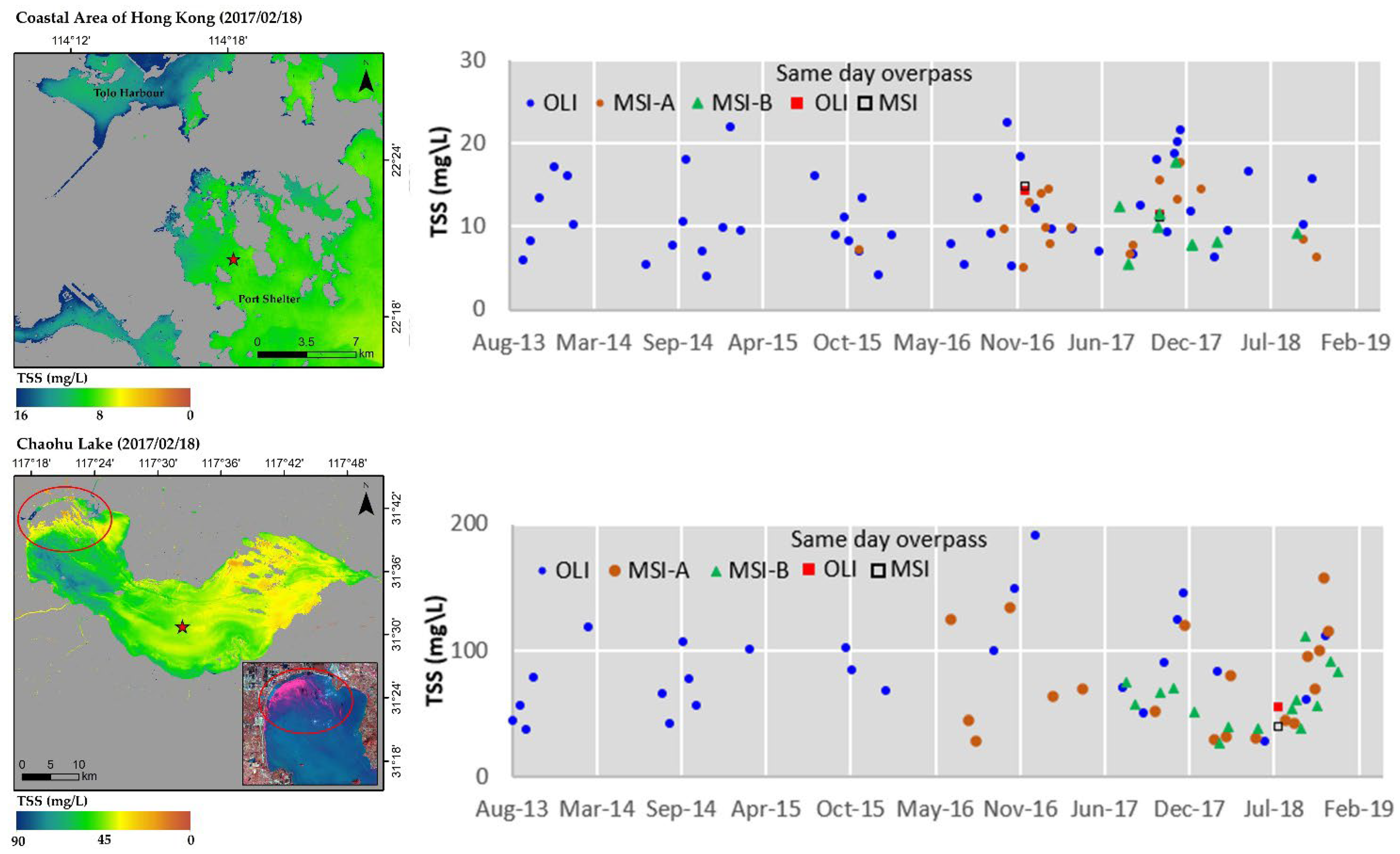
This section covers: (i) a brief overview of the test area; (ii) relative spatial accuracy; (iii) an explanation of atmospheric correction (AC) using vicarious calibration gains; and (iv) spectral consistency assessment. This section also includes examples of combined use of the OLI and the MSI for aquatic applications such as (i) time series analysis of the TSS concentrations; (ii) algae bloom area intercomparison; and (iii) the tracking of floating algae. Here, we refer to both MSI sensors onboard S-2 A/B as the MSI, but to be specific, MSI-A or MSI-B refer to their satellites, when necessary.

2.1. Testing Area

Only a few large lakes in China can be monitored using low-resolution satellite data like MODIS and the Sentinel-3 Ocean and Land Colour Instrument (OLCI). However, there are around 3000 lakes with areas of more than 1 km2, and most of them belong to case Ⅱ waters featuring a large volume of shallow waters [41]. Low-resolution data are not sufficiently reliable when it is adopted to monitor these small and average-size lakes. Furthermore, an investigation conducted in 2013 by the Ministry of Ecology and Environment in China showed that 57.4% of the lakes surveyed were eutrophic, with an extra 27.8% in a hypereutrophic condition [42]. Most lakes in the northeastern China are highly eutrophic, and algae bloom events are quite common in these lakes. Furthermore, the Chinese coastal area is the home ground of the largest fishing industry in the world, and its annual contribution to China’s food supply is over 57 million metric tons, and the industry provides over 9.2 million jobs [43]. Eutrophication caused by the nutrient enrichment and frequency of harmful algae blooms has displayed a steady trend, posing a threat to the coastal activities in these waters [5]. Therefore, the inland and coastal waters of China were selected for this study. Figure 1a–k shows the test sites. Eight diverse, oligotrophic-eutrophic lakes and three coastal regions were selected for the current study. Lake Taihu, Lake Hongze, Lake Chaohu, Lake Dianchi, and Lake Poyang are eutrophic [42], while Lake Ulungur, Lake Ebinur, and Qinghai Lake are oligotrophic. Qinghai Lake is also one of the calibration sites for space-borne remote sensors [44]. Water in the Yangtze River estuary is highly turbid, while moderate-to-low turbid in the Lianyungang coastal area and the Hong Kong coastal area.

2.2. Dataset

L-8 and S-2 A/B have 185 km and 290 km fields of view, respectively, with equatorial crossing times at 10:00 a.m. ± 15 min and 10:30 a.m., are placed in orbits such that they occasionally capture the same area on Earth simultaneously with <30 min time difference [45,46]. Both satellites provide data with a radiometric quantization of 12 bit. Details of satellite sensors are given in Table 1. Overall, 46 near-simultaneous nadir overpass images, 20 by L-8 and 26 by S-2 A/B, were selected for 11 test sites. Near-simultaneous images with time difference of ≤25 min were considered. We selected scene pairs with low/no cloud cover and low aerosol loading. Level-1 C MSI and level-1 T OLI data were acquired from ESA’s Copernicus Open Access Hub and Earth Explorer over the test sites, respectively. The images used in this study are given in Table S1 of the Supplementary Materials.

2.3. Data Processing

Figure 2 shows the workflow of data processing for consistency assessment. The following subsections cover the details of data processing.

2.3.1. Relative Co-Registration Test

Both satellite images were first projected to the same projection system. Before the relative co-registration test, MSI data were resampled to 30 m resolution to match the OLI pixel dimensions. Sixty benchmarks were collected regularly over 12 image pairs, mainly from marine structures or water channels entering inland/coastal waters. Co-registration among OLI and MSI data was tested as follows:
The difference between Easting ( Δ E) and Northing ( Δ N) was calculated for all the benchmarks; mean ( m Δ E , m Δ N ) and standard deviation values ( S Δ E , S Δ N ) were computed; m Δ E , m Δ N were considered as a measure of bias and S Δ E , S Δ N were considered as a measure of precision. In the relative co-registration test, bias is the relative difference between two datasets. Bias is assumed negligible if standard deviation < mean. The total error of the generic point was as follows:
Δ i = Δ E i 2 + Δ N i 2
The root-mean-square error (RMSE) was considered as a synthetic measure of accuracy:
RMSE = 1 n i = 1 n Δ i 2
where n is the total number of benchmark points.

2.3.2. Atmospheric Correction and Masking

Acolite Python version 20180925.0 [47] was adopted to derive calibrated ρ t ,   ρ r c ,   R r s . Acolite is designed for correcting Landsat (5–9) and S-2 A/B images for coastal and inland water applications [47]. It includes the dark spectrum fitting (DSF) [48] and exponential extrapolation (EXP) [49] methods for atmospheric correction. For the L-8 OLI and the S-2 MSI, it is recommended to use the recently developed DSF method. In addition to atmospheric correction, Acolite also includes already developed models as in-built models which can be adopted to retrieve several water quality parameters, i.e., Chl-a, TSS, and turbidity. Vicarious calibration gains reported by Pahlevan et al. [50] were used for OLI data, and gains reported by Pahlevan et al. [11] were used for MSI-A and MSI-B in the Acolite software. A unit gain was used for the 492 nm band of MSI-A as recommended [11]. No sun-glint correction method was applied in Acolite. The SWIR-I band (at 1600 nm) with threshold 0.0215 was adopted in masking land, cloud, and sun glint pixels, as it is proven to be effective in discriminating land and cloud from water pixels, even in turbid coastal waters [51]. Currently, Acolite has resampling capability only for the MSI. Therefore, only the MSI was resampled to 60 m resolution, and OLI data retained their original resolution after processing.

2.3.3. Spectral Consistency Assessment

Spectral consistency assessment was performed at two levels, i.e., level 1 ( ρ t , ρ r c ) and level 2 ( R r s ) for matching bands of OLI and MSI-A and MSI-B using simultaneous same-day data. Pixels pairs for spectral consistency analysis were selected from test sites (Figure 1 and Table S1) such that pixels were 100 m distant from land and one pair was at least 500 m apart from the next one. To minimize the effects of the BDRF (bidirectional reflectance distribution factor), pixels within ±7° of the view zenith angles were selected. To avoid the computational burden, a maximum of 300 matchups for each scene pair were considered. Matchup pixels with cloud shadow were dropped carefully as the masking algorithm does not work well if the cloud shadow exists, it is reported as clear water. Data from both sensors (OLI/MSI) were resampled to 60 m to minimize random noise and/or artefacts before the extraction of band values from coeval MSI and OLI data. Spectral values for the non-masked area (water pixel) were adopted for ρ t ,   ρ r c , and R r s comparison. A large dataset comprising 4409 and 542 matchups was selected for comparing level-1 OLI data with MSI-A data, and level-1 OLI data with MSI-B data, respectively. For level-2 product comparison, 4409 and 408 matchups were selected from same-day overpass pairs for the OLI–MSI-A and the OLI–MSI-B comparison, respectively.
Spectral band differences were expressed in terms of the root-mean-square error (RMSE), the mean absolute percentage error (MAPE), and the median difference (MD) (Equations (3)–(5)). The median was preferred over the mean in case there were any outliers and any noise present in the data due to atmospheric correction or difference in the spectral response function.
RMSE = 1 N ( ρ   S 2 ( λ i ) ρ     L 8 ( λ i ) ) 2
MAPE = 100 × 1 N       | ρ   L 8 ( λ i ) ρ S 2 ( λ i ) | ρ   L 8 ( λ i )
MD = Median   ( ρ S 2 ( λ i ) ρ   L 8 ( λ i ) )
where ρ   denotes   ρ t ,   ρ r c ,   or   R r s ,   S 2 ( λ i )   denotes the band i value recorded by the S-2 MSI-A or S-2 MSI-B, L 8   ( λ i )   denotes the band i value recorded by the L-8 OLI, and N is the total number of matchup pixels.
For spectral band adjustment, the abovementioned condition (view zenith angles within ±7°) was not considered, and matchups from overlapping areas of L-8 and S-2 were collected (i.e., 11,000 for L-8 and S2-A and 6000 for L-8 and S2-B). The linear regression model was used using L-8 as reference data for the spectral adjustment that was calibrated using 70% of the data and evaluated using 30% of same-day data. The linear regression method is also applied to synthetic data of surface reflectance processed from a large number of hyperspectral EO-1 Hyperion scenes for deriving harmonized Landsat-S-2 surface reflectance products [52]. The spectral band differences after band adjustment were expressed in terms of the RMSE (Equation (2)). The RMSE reduction rate (RRR) was used to quantify the cross-sensor consistency improvement as follows:
RRR = ( RMSE RMSE ) RMSE × 100
where RMSE and RMSE refer to the spectral difference before and after band adjustment.

2.3.4. Combined Landsat-8/OLI and Sentinel-2/MSI Use for Coastal/Inland Water Applications

This section covers some case studies considering coastal and inland water applications where data from the L-8 and S-2 virtual constellation can be used for detailed monitoring.
i.
Example 1: TSS time series analysis
Through time series analysis, the TSS consistency for same-day overpass is explained, and the analysis also serves as a way of showing how MSI-A and MSI-B fill data gaps in inland and coastal areas, making it possible to study the dynamic behavior of these resources. For time series analysis, one lake area (Lake Chaohu) and one coastal area (Port Shelter coastal area of Hong Kong) were selected. A total of 58 OLI, 29 MSI-A, and 13 MSI-B cloud-free images were used in time series analysis over the coastal area of Hong Kong (Table S2). Similarly, 53 OLI, 27 MSI-A, and 18 MSI-B images were used in time series analysis at Lake Chaohu, China (Table S3). The TSS algorithm by Nechad et al. [53] was used in this study. This algorithm was recalibrated for the OLI and the MSI and embedded in Acolite version 20180925.0. Data from all the sensors were resampled to 60 m prior to applying the TSS algorithm.
ii.
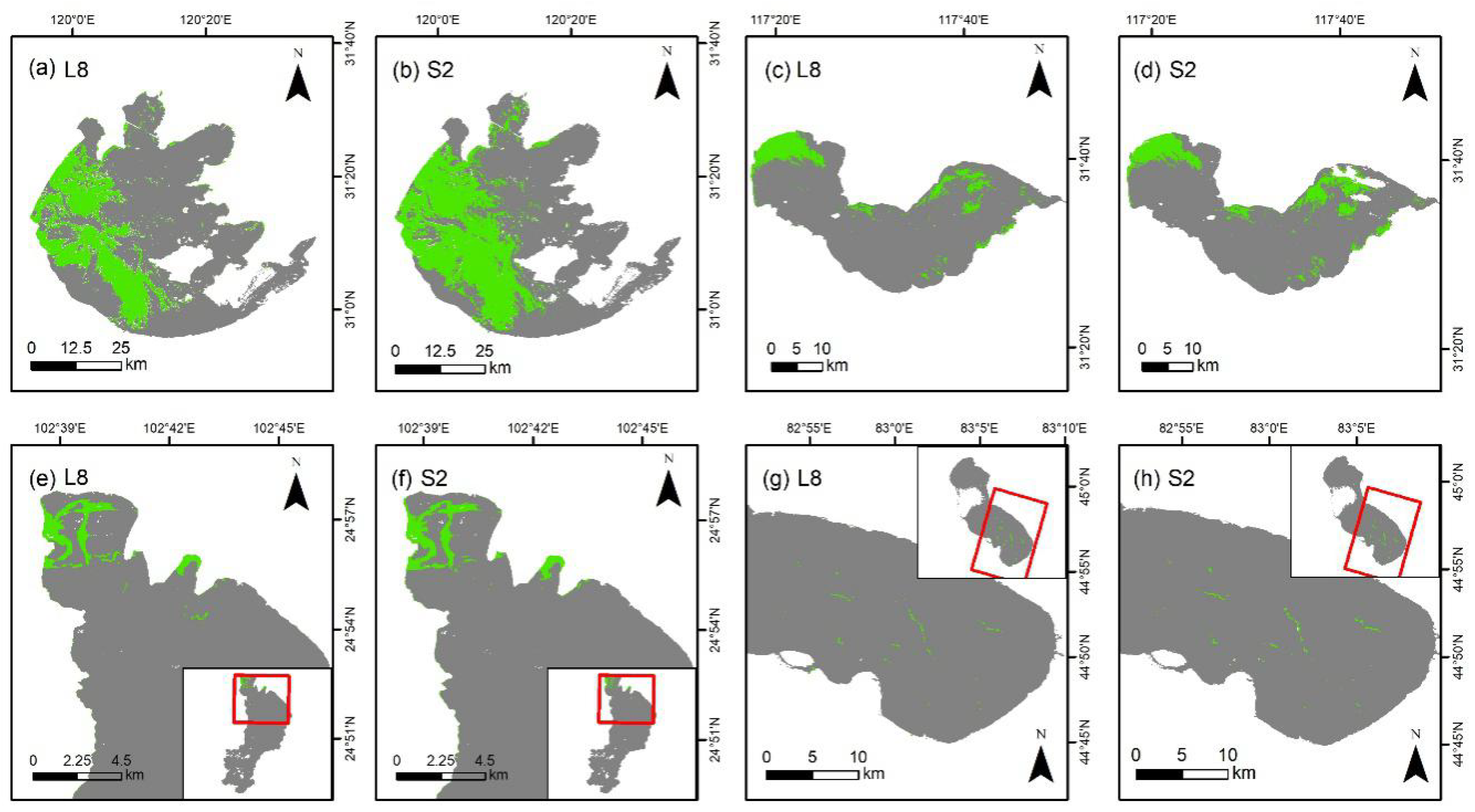
Example 2: Floating algae area comparison
The floating algae area was extracted by incorporating the floating algae index (FAI) [54] (Equations (7) and (8)). The FAI has been found to be relatively stable as compared to the NDVI and enhanced vegetation index (EVI), especially with respect to atmospheric turbidity [54]. Cloud-free Rayleigh-corrected OLI and MSI data were used to derive the FAI from four lakes, Lake Taihu, Lake Chaohu, Lake Dianchi, and Lake Ebinur. The data were further classified based on the FAI threshold (FAI > 0) to algal and non-algal pixels. For each lake, surface reflectance in the SWIR-I band of the cloud-free image was adopted to extract the feature boundary of inland water. The threshold value of 0.0215 was used to separate water from the land area. The data used for FAI analysis are shown in Table S4.
FAI = ρ r c , N I R ρ r c , N I R
ρ r c , N I R = ρ r c , R E D + ( ρ r c , S W I R ρ r c , R E D ) . λ N I R λ R E D λ S W I R λ R E D
iii.
Example 3: Tracking of coastal floating algae
The Yellow Sea, 35°0′N 123°0′E, is a semi-closed sea and is usually affected by floating algae in the summer. The floating algae area was extracted using all available OLI and MSI data collected in June and July (2019). A total of 83 OLI, MSI-A, and MSI-B images were adopted (Table S5). The floating algae area was extracted based on the methodology explained in Section 2.3.4.

3. Results

3.1. Geometric Assessment

Relative geometric assessment between OLI and MSI data was assessed using the mean ( m Δ E , m Δ N ), standard deviation ( S Δ E , S Δ N ), and the RMSE. Statistics (Table 2) show that no systemic errors were present since m Δ E and m Δ N remained lower than the corresponding S Δ E and S Δ N . Furthermore, the RMSE was 23.5 m, which is less than the OLI pixel size (30 m), ensuring that spectral measures from OLI and MSI data refer to the same ground point and therefore represent the same type of surface.

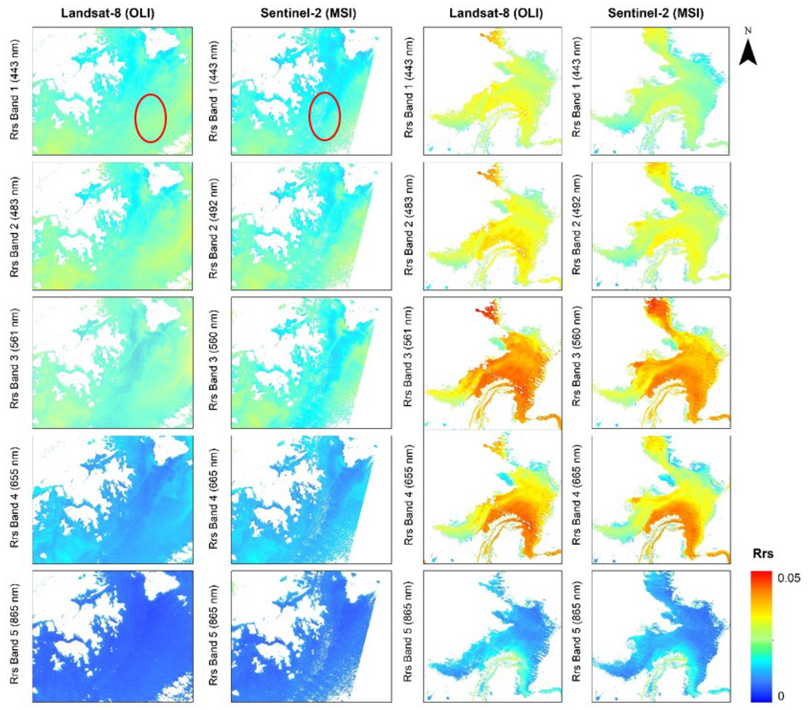
3.2. Spectral Consistency Assessment

The OLI and MSI-A/B data were corrected for atmospheric effects using Acolite software [49]. Acolite has been demonstrated with reasonable results for the OLI [23,55] and the MSI [56] for water quality applications. Figure 3 presents the initial comparison of the OLI and the MSI-A ( R r s )   in a coastal region and an inland region. The lower and higher limits and the spatial variation of R r s   for the OLI and MSI-A bands are consistent across these test sites. However, the OLI produced higher values as compared with the MSI-A values over relatively less turbid coastal waters in band 1 (area indicated by an ellipse in Figure 3). For detailed assessment, band-by-band consistency comparison for the same-day OLI–MSI-A/B level-1 and level-2 products are discussed in this section. The OLI–MSI-A and OLI–MSI-B pixel pairs were compared separately to access the consistency. Band agreements are displayed using scatterplots (Figures S1–S6 of the Supplementary Materials) where the 1:1 line represents perfect agreement between the sensor bands and allows visual assessment of misalignment between two sensors.

3.2.1. Top-of-Atmosphere Reflectance ( ρ t )

With the values of the slope, intercept, and coefficient of determination (R2), it is possible to evaluate the consistency of OLI and MSI products. R2 is high, ≥0.80, in all the bands for OLI and MSI-A pairs. R2 is also high, ≥0.80, for all the visible and NIR bands for OLI and MSI-B pairs. The highest R2 was observed in the green band for OLI and MSI-A pairs (OLI: 561 nm, MSI-A: 560 nm) and in the red band for OLI and MSI-B pairs, although the red band did not fully overlap (OLI: 655 nm, MSI-B: 665 nm). The product difference in terms of the MAPE (MAPE in all the channels except SWIR bands) was ≤5% and ≤8% for the OLI–MSI-A and OLI–MSI-B comparison, respectively. The MAPE is lowest in band 3 (2.0 % in the OLI–MSI-A pair and 1.5% in the OLI–MSI-B pair) and highest in SWIR bands ≥ 13.5%. The corresponding slope, intercept, RMSE, MD, and MAPE for each band for OLI–MSI-A and OLI–MSI-B pairs are summarized in in Table 3. Scatterplots for OLI–MSI-A and OLI–MSI-B comparison are given in Figure S1. Large ρ t -NIR values were observed during the occurrence of algae bloom events.

3.2.2. Rayleigh-Corrected Reflectance ( ρ r c )

The values of the slope, intercept, and R2 show that Rayleigh-corrected reflectance ( ρ r c   )   is also consistent in visible and NIR bands, with R2 ≥ 0.87 for all the test sites (Table 4). The highest R2 (0.99) was observed in the green band, with low MAPE (3.4%) for the OLI–MSI-A comparison. The green band also showed the highest consistency for the OLI–MSI-B comparison (R2 = 0.98, MAPE = 2.3%). Table 4 shows slope, intercept, RMSE, MD, and MAPE for each band in the OLI and the MSI-A/B. The scatterplot of ρ r c   (NIR) shows that the values are almost consistent for NIR < 0.06, and the inter-consistency between the OLI and the MSI-B decreases with higher NIR values (Figure S4). Large ρ r c (NIR) values are observed during the occurrence of algae bloom events. Rayleigh-corrected red, NIR, and SWIR bands are important for the detection of floating algae during algae bloom events, as floating algae reflect significantly in the NIR portion of the spectrum [54]. The average MAPE in the coastal aerosol band is high as compared to visible and NIR bands for OLI–MSI-A/B comparison. This uncertainty could be attributed to pixel size difference (60 m in the MSI-A/B and 30 m the OLI) or error in atmospheric correction. High MAPE was observed in SWIR bands. These differences may have been due to differences in the signal-to-noise ratio (SNR) or spectral range differences of SWIR bands.

3.2.3. Water-Leaving Remote-Sensing Reflectance ( R r s )

Remote-sensing reflectance ( R r s = ρ w / p i ; ρ w   i s   water-leaving-reflectance) data are critical for water quality algorithm development. Satellite-based ρ w   or   R r s products are adopted in several studies to develop models for retrieving different water quality parameters [16,57,58]. A research study was also conducted to map water clarity with combined OLI and MSI data and perform single model calibration and validation [16]. The assessment of inter-sensor consistency in R r s is important before the combined use. The R r s comparison shows the consistencies between OLI and MSI data (Table 5). Like the ρ t and ρ r c   comparison, the green band was highly consistent with the lowest MAPE in the OLI–MSI-A and OLI–MSI-B comparison. Overall, a higher R2 was found in green and red channels. The MAPE is highest in band 1 for both comparison datasets. The reason behind low consistency can be pixel size differences (60 m in the MSI-A/B and 30 m in the OLI) or an error in atmospheric correction. Pahlevan et al. [59] suggested that if ambient aerosol properties are not considered, high uncertainty in R r s (443) is expected.

3.3. Spectral Band Adjustment

A linear regression model (using 70% band pair data) was suggested in this study for spectral band adjustment. With the coefficients mentioned in Table 6 and Table 7, band 1–4 and band 9 of MSI-A/B was adjusted to fit the OLI spectral values. After band adjustment, we recalculated the R2 the RMSE’. and the RRR for test data (30%). Table 6 and Table 7 show that bias removal determines an appreciable improvement in spectral consistency of OLI–MSI-A and OLI–MSI-B. The adjustment in MSI-A data shows that the RMSE in visible bands increased significantly with higher RRR in coastal aerosol and the blue band for ρ t and the highest RRR was observed for the NIR band when ρ r c and R r s were adjusted for the OLI. The RRR was also high for the coastal aerosol band and the blue band when MSI-B bands were adjusted. Additionally, RRR was also high when MSI-B data were adjusted for the OLI red band. Overall RRR values show that a linear regression model can be used to adjust MSI-A and MSI-B data to fit OLI spectral data with a considerable decrease in the RMSE. To further remove the bias, the researcher also suggested applying normalization when multi-sensor data (OLI and MSI-A/B) were under consideration for the same statistical distribution [30].

3.4. Example 1: Time Series Analysis

The utility of combined OLI–MSI products is discussed by assessing the time series of the TSS in a coastal region and a lake region under diverse atmospheric and aquatic conditions. Figure 4 shows the time series plots which exhibit valid TSS retrievals from August 2013 (after the launch of the OLI). These plots show diverse seasonal variability between the TSS in the coastal area of Hong Kong and Lake Chaohu. The arbitrary point was selected for TSS data extraction from both sites. The extraction was conducted by taking the mean over the 4 × 4 and 6 × 6 averaging window (equivalent to 120 m2) from OLI and MSI data, respectively. The location of the arbitrary point was arranged in such a way so as to ensure the window sizes mentioned above were not affected by the pixels adjacent to the land/cloud shadow. The analysis of two different aquatic systems, coastal and inland, illustrated with different TSS concentrations, highlighted the value of the combined use of the OLI and the MSI. Time series plots clearly show that MSI data fill the gap of OLI data. For instance, there is a visible data gap from January to July 2014, and from January to July 2015, in both areas. This gap started to be filled partially after the launch of the MSI-A. Data from the MSI-B fill more data gaps. It can be seen from both plots that the cloud-free data availability after June 2017 has increased. The solid red square and the black hollow square represent the same-day overpass (<25 min time difference). Two overpasses revealed that the TSS products estimated by the OLI were slightly higher than the ones estimated by the MSI. The TSS concentration range varied from 5–25 mg/L in the port shelter coastal area of Hong Kong. High values are recorded during the winter season. TSS concentration values are large at Lake Chaohu from 20 to 190 mg/L. Triplets of the sensors evidently capture the seasonal variability across these areas, with the TSS peak occurring in December 2017 in the coastal area of Hong Kong, and the TSS peak occurring in December 2017 and November 2018 at Lake Chaohu. Jiang, et al. [60] also observed an average of 31.1 ± 20.78 mg/L during summer months (May–August), which is comparable to the results for this time series analysis. The same-day overpass data were not adequate for the performance of the statistical analysis. Further research is required to quantify the errors in the OLI, MSI-derived TSS using in-situ TSS data; and calibration and validation of TSS algorithm using combined OLI-MSI data.

3.5. Example 2: Floating Algae Area Comparison

The advantages of the spatial resolution of MSI (10–20 m) and OLI (30 m) data for the mapping of floating algae areas at four diverse lakes using same-day overpass data are discussed in this section. Figure 5 and Figure 6 show the comparable algae area derived from the same-day OLI and MSI data. The floating algae area is slightly higher in MSI products in all the lakes except Lake Taihu. MSI data led to the largest difference in the algae area of 268 km2 at Lake Taihu. This large difference in the area can be attributed to the largest time difference (19 min) between overpasses. MSI-A data were 19 min ahead, and algae bloom grew more rapidly where there were favorable environmental conditions, such as higher temperature, exposure to light, and suitable wind. The time difference is 7 min at Lake Chaohu, 4 min at Lake Dianchi, and 12 min at Lake Ebinur. This analysis shows the competency of higher MSI spatial resolution and the benefits of the combined use of OLI and MSI data.
With a high resolution of the OLI and the MSI (10–30 m) as compared to the MODIS (500–1000 m) and the OLCI (300 m), relatively accurate floating algae area as the MODIS and the OLCI can be provided, and the algal pixel can be detected as non-algal due to mixed pixel effect or vice versa can be detected. Of these four lakes, serious eutrophication was observed at Lake Taihu and Lake Chaohu [61,62], which are the third and fifth largest freshwater lakes in China, respectively. The monitoring of cyanobacterial blooms at Lake Taihu started in 2008. Since then, an increase in the affected area has been reported by researchers [61,63]. A comprehensive study based on fourteen-year MODIS data archive at Lake Chaohu also found an increase in the surface algae bloom frequency, bloom coverage, and duration [62]. Lake Chaohu is the major potable water resource for the Hefei City, but due to the reoccurrence of massive algae blooms, the water resource was changed to Dongpu reservoir [4]. Algae blooms of different seriousness take place every year, but the upper part of Lake Dianchi displays higher algae bloom frequency [64], and the water of Lake Ebinur is relatively clear with occasional occurrences of thin algae slicks.

3.6. Example 3: Tracking of Coastal Floating Algae

Accurate and timely detection of coastal floating algae (FA) and tracking of bloom time are relatively difficult if the traditional ocean color satellite data are adopted and the surface area of FA is relatively small in the start and the end of bloom. Reliable revisit frequency of the OLI and the MSI with high-resolution data provides an opportunity to track the record of the accurate coastal area affected by FA. However, the coverage area of the MSI and the OLI is limited when the open sea is considered. Here, this analysis provides insight into the tracking of coastal FA during June and July 2019 based on the combined use of OLI and MSI-A/B data. Figure 7 shows the changes in FA in the two months. The bloom started in the lower (33.6°N 122.1°E) and central (35.7°N 120.9°E) parts of the Yellow Sea in the beginning of June and persisted in this part until the end of June (Figure 7: upper blue box). The bloom also grew in the northern part (36.3°N 121.1°E) by the end of June (Figure 7: upper red and black box), and coastal areas of Yancheng were also affected. In early July, the bloom area moved a little eastward, and in mid-July, more FA appeared near the coastal areas of Qingdao (Figure 7: lower red and black box). These changes in FA are attributed to both new FA growth and/or its movements caused by currents. At the start of the bloom, the maximum width of a floating algal slick was 700 m, which is difficult to be detected by a traditional ocean color sensor. The width of an algal slick increased to 6000 m during the peak bloom.

4. Discussion and Future Directions

Integrated Landsat-8/9 and Sentinel-2 data open new opportunities for monitoring coastal and inland waters at a frequency that has never been possible before because the temporal coverage at 10–60 m spatial resolution can be improved with combined use. The resulting increase in the average revisit time, as well as in the number of cloud-free images, can guarantee better monitoring of the dynamics of inland and coastal waters [11]. Furthermore, the combined use of these satellite sensors provides a great opportunity to build time series with an improved spatial and temporal resolution [26], thus enabling limnologists, aquatic ecologists, coastal oceanographers, and water resource managers to enhance their monitoring efforts [10,21]. NASA scientists have developed a harmonized Landsat and S-2 (HLS) surface reflectance product [31]. Although the HLS product is a free and valuable opportunity to create combined OLI–MSI datasets, there are some shortcomings, which hamper its utilization by the ocean color community. In general, HLS products are mostly designed for land applications [65], and the atmospheric correction method adopted does not correct for the adjacency effect, the sun-glint effect, etc., i.e., the main issues concerning water applications using satellite data. Furthermore, the HLS data are available only for selected sites (120 worldwide), so the combined OLI–MSI application is not possible everywhere in the world. A study by Shang and Zhu [65] discusses the OLI–MSI data consistency and time-series based on the reflectance adjustment approach. However, they masked the water and snow/ice data to focus on land surface reflectance. Pahlevan et al. [11] evaluated OLI–MSI spectral consistency for aquatic application considering multiple inland and coastal regions around the world. However, they considered limited view zenith and azimuth angles during data extraction to minimize the effects of the bidirectional reflectance distribution factor. Moreover, Runge and Grosse [39] suggested that localized harmonized OLI–MSI data can be generated through the least square regression for the adjustment of the spectral band. Therefore, in this study, the spectral consistency OLI–MSI data were evaluated, and afterwards the capability of combined OLI–MSI data for TSS time series, algae bloom area mapping, and tracking of floating coastal algae bloom was discussed.
Spectral consistency analysis shows that OLI and MSI products, ρ t ,   ρ r c ,   and   R r s   , are adequately consistent. The products’ differences are ~8% in ρ t and ~10% in both ρ r c   and R r s   for all the matching bands. Overall, the lowest RMSE and MAPE were found in the green band for level-1 and level-2 products for both OLI–MSI-A and OLI–MSI-B comparisons. The difference in some matchups in the NIR band can be attributed to the occurrence of rapid algae bloom changes caused by the time difference between L-8 and S-2 overpasses. The algae may grow readily under changing light conditions; therefore, consistency in NIR values tends to decrease as the time difference between same-day overpasses increases. Our finding on R r s   (OLI: 655 nm; MSI: 665 nm) agrees well with the corresponding results provided by Ciancia et al. [66]. The spectral consistency analyses by Pahlevan et al. [11] were based on the image products processed via SeaDAS, and they suggest that the relative consistency in OLI–MSI products, which are processed through other available processing systems, should be studied, especially in extremely eutrophic/turbid conditions and/or CDOM-rich waters where SeaDAS retrievals often fail. In this study, spectral consistency analysis was performed with the use of image products processes via Acolite [47]. Acolite is an atmospheric correction algorithm and processing software developed at RBINS for aquatic applications of Landsat (5–9) and S-2 (A/B) satellite data. Acolite can not only be adopted to perform atmospheric correction but can also retrieve several water quality parameters derived from water reflectance.
The assessment of TSS variability plays a key role in inland and coastal water management and tries to answer questions such as how these fluctuations influence water clarity, light availability, and the physical, chemical, and biological processes (such as primary production) [13,58,67]. In this study, the time series constructed based on the combined use of OLI–MSI data further emphasize the effectiveness and consistency of L-8 and S-2 missions. No band adjustment algorithm was used before retrieving the TSS from either sensor. Analysis showed that overall, the TSS concentrations derived from OLI data were slightly higher than MSI-A/B data. Algae bloom area comparison also showed consistent results. However, the difference in the algae bloom area increased as the time difference between the same-day overpass images increased. Moreover, tracking of floating algae bloom using available cloud-free OLI and MSI data reveals interesting results in case of open sea, despite their lower swath coverage as compared to traditional ocean color sensors. Small algal slicks (width ~700 m), at the start of the two-month long algae bloom event, were accurately identified, which is quite impossible if the traditional ocean color satellite is adopted. Coastal oceanographers and aquatic ecologists can precisely identify the location and season which are more favorable for algae bloom events by taking advantage of high-resolution OLI–MSI data.
It is important to use consistent algorithms for consistent product records for Landsat and Sentinel-2 missions. Both sensors have their distinct advantages such as the MSI has additional red edge bands (705, 740, and 783 nm) which allow the application and development of alternative algorithms for Chl-a retrievals in hypereutrophic systems [17,18], whereas the OLI has a panchromatic band which enables it to identify cyanobacteria biomass by the detecting phycocyanin pigment using the orange contraband (620 nm). Further studies should also emphasize the limitations and advantages of product consistency, band adjustment approaches for consistent products and improve water quality parameters (e.g., Chl-a, TSS, CDOM) retrievals by combined use. As the S-2-MSI can produce more robust Chl-a records by taking advantage of additional red edge bands and its higher spatial resolution than that of the L-8/9 OLI, an S-2-based independent algorithm can be used separately in hypereutrophic waters while another set of consistent algorithms can be applied to both L-8/9 and S-2 data to produce consistent Chl-a or other water quality parameters such as water clarity [16], TSS, or algae bloom area record.

5. Conclusions

The present study aims to evaluate the inter-sensor consistency for Operational Land Imager (OLI) and Multispectral Imager (MSI), Level-1 and level-2 products which are important for the generation of aquatic ocean color products for inland and nearshore coastal waters. The dark spectrum fitting method in Acolite was adopted for atmospheric correction. This demonstration was performed at a near-simultaneous same-day overpass allowing for almost similar atmospheric conditions. The study shows that vicariously calibrated OLI and MSI-A/B average products difference is ~8% in ρ t   ,   and   ~10% in ρ r c   and R r s   for all matching bands, and ~3.7% in ρ t , ~5.7% in ρ r c   and ~7.5% in R r s for all visible bands except the coastal aerosols band. The lowest MAPE was found in green band for level-1 and level-2 products for both OLI–MSI-A and OLI–MSI-B comparison. The linear regression model showed that RMSE has decreased significantly after band adjustment with the highest reduction rate in NIR band and red band for OLI-MSIA and OLI-MSIB comparison. Consistency in total suspended solids (TSS) for same-day has also been evaluated for various water types. Time series in the coastal and inland waters provide detailed insight into the TSS derived from OLI and MSI-A/B with MSI producing slightly lower TSS, while there is a need for more in-situ data to evaluate OLI and MSI derived TSS over test sites. Triplets of satellites, with two to three days revisit time, provide more data enabling end-users to derive consistent water quality products, with reliable resolution and further investigation of seasonal trends. Floating algae bloom area extraction was performed using same-day OLI and MSI-A/B data. The analysis reveals that the difference in the algae area increases with the time difference between the same-day overpass. Coastal algae bloom tracking using available OLI and MSI data shows the application of these satellites reveals interesting results in case of open sea, despite their lower swath coverage as compared to traditional ocean color sensors. Further, the reliable resolution of OLI and MSI is capable of detecting thin algal slicks. Although results suggest that the S-2 MSI and L-8/9 OLI products at level 1 and level 2 are consistent and can be used qualitatively, and quantitatively, for monitoring inland and nearshore coastal waters. Nonetheless, further research efforts are needed: to develop band adjustment approaches to minimize the product difference, improve atmospheric correction models, and suitable biogeochemical algorithms to maximize the synergy use of these sensors.

Supplementary Materials

The following supporting information can be downloaded at: https://0-www-mdpi-com.brum.beds.ac.uk/article/10.3390/rs14133155/s1, Figure S1: Inter-comparison of Top of atmosphere reflectance (ρ_t) for OLI – MSI-A pairs; Figure S2: Inter-comparison of Top of atmosphere reflectance (ρ_t) for OLI – MSI-B pairs; Figure S3: Inter-comparison of Rayleigh corrected reflectance (ρ_rc) for OLI – MSI-A pairs; Figure S4: Inter-comparison of Rayleigh corrected reflectance (ρ_rc) for OLI – MSI-B pairs; Figure S5: Inter-comparison of remote sensing reflectance (R_rs) for OLI – MSI-A pairs; Figure S6: Inter-comparison of remote sensing reflectance (R_rs) for OLI – MSI-B pairs; Table S1: Landsat 8 OLI and Sentinel 2-MSI A/B near- simultaneous overpass images used for spectral consistency analysis and band adjustment; Table S2: Landsat-8 OLI and Sentinel 2-MSI A/B images used for Total suspended solids (TSS) time series analysis over Hong Kong; Table S3: Landsat-8 OLI and Sentinel 2-MSI A/B images used for Total suspended solids (TSS) time series analysis over Lake Chaohu; Table S4. Landsat-8 OLI and Sentinel 2-MSI A/B images used for floating algal area comparison; Table S5. Landsat-8 OLI and Sentinel 2-MSI A/B images used for floating algal bloom tracking over the Yellow Sea.

Author Contributions

Conceptualization: S.H. and M.S.W.; Analysis: S.H.; Writing—original draft preparation: S.H.; Writing–review and editing: S.H., M.S.W., S.A. and M.A.; Funding acquisition, M.S.W. All authors have read and agreed to the published version of the manuscript.

Funding

This research was supported in part by the General Research Fund (project ID 15609421 and 15603920), and the Hong Kong Ph.D. Fellowship Scheme from the Research Grants Council of Hong Kong. M. S. Wong thanks the support from the Research Institute for Land and Space (project ID 1-CD81), The Hong Kong Polytechnic University.

Data Availability Statement

The data presented in this study are available on request from the corresponding author.

Acknowledgments

The authors would like to acknowledge the US Geological Survey (USGS) and the Copernicus Open Access Hub European Space Agency (ESA) for providing the Landsat-8 (OLI) and Sentinel-2 image archive. Furthermore, the authors would like to thank the reviewers and editors for their time and valuable input to this manuscript.

Conflicts of Interest

The authors declare no conflict of interest.

References

  1. Small, C.; Nicholls, R.J. A global analysis of human settlement in coastal zones. J. Coast. Res. 2003, 19, 584–599. [Google Scholar]
  2. Paerl, H.W.; Paul, V.J. Climate change: Links to global expansion of harmful cyanobacteria. Water Res. 2012, 46, 1349–1363. [Google Scholar] [CrossRef] [PubMed]
  3. Hallegraeff, G.M. A review of harmful algal blooms and their apparent global increase. Phycologia 1993, 32, 79–99. [Google Scholar] [CrossRef] [Green Version]
  4. Xie, P. Reading about the Histories of Cyanobacteria, Eutrophication and Geological Evolution in Lake Chaohu; Science Press: Beijing, China, 2009. (In Chinese) [Google Scholar]
  5. Mackey, K.R.M.; Kavanaugh, M.; Wang, F.; Chen, Y.; Liu, F.; Glover, D.M.; Chien, C.-T.; Paytan, A. Atmospheric and Fluvial Nutrients Fuel Algal Blooms in the East China Sea. Front. Mar. Sci. 2017, 4, 2. [Google Scholar] [CrossRef] [Green Version]
  6. Chen, X.; Li, Y.S.; Liu, Z.; Yin, K.; Li, Z.; Wai, O.W.; King, B. Integration of multi-source data for water quality classification in the Pearl River estuary and its adjacent coastal waters of Hong Kong. Cont. Shelf Res. 2004, 24, 1827–1843. [Google Scholar] [CrossRef]
  7. Doña, C.; Chang, N.-B.; Caselles, V.; Sánchez, J.M.; Camacho, A.; Delegido, J.; Vannah, B.W. Integrated satellite data fusion and mining for monitoring lake water quality status of the Albufera de Valencia in Spain. J. Environ. Manag. 2015, 151, 416–426. [Google Scholar] [CrossRef] [Green Version]
  8. Li, J.; Roy, D.P. A Global Analysis of Sentinel-2A, Sentinel-2B and Landsat-8 Data Revisit Intervals and Implications for Terrestrial Monitoring. Remote Sens. 2017, 9, 902. [Google Scholar] [CrossRef] [Green Version]
  9. Tyler, A.N.; Hunter, P.D.; Spyrakos, E.; Groom, S.; Constantinescu, A.M.; Kitchen, J. Developments in Earth observation for the assessment and monitoring of inland, transitional, coastal and shelf-sea waters. Sci. Total Environ. 2016, 572, 1307–1321. [Google Scholar] [CrossRef] [Green Version]
  10. Pahlevan, N.; Sarkar, S.; Franz, B.; Balasubramanian, S.; He, J. Sentinel-2 MultiSpectral Instrument (MSI) data processing for aquatic science applications: Demonstrations and validations. Remote Sens. Environ. 2017, 201, 47–56. [Google Scholar] [CrossRef]
  11. Pahlevan, N.; Chittimalli, S.K.; Balasubramanian, S.V.; Vellucci, V. Sentinel-2/Landsat-8 product consistency and implications for monitoring aquatic systems. Remote Sens. Environ. 2019, 220, 19–29. [Google Scholar] [CrossRef]
  12. Pahlevan, N.; Lee, Z.; Wei, J.; Schaaf, C.; Schott, J.R.; Berk, A. On-orbit radiometric characterization of OLI (Landsat-8) for applications in aquatic remote sensing. Remote Sens. Environ. 2014, 154, 272–284. [Google Scholar] [CrossRef]
  13. Liu, H.; Li, Q.; Shi, T.; Hu, S.; Wu, G.; Zhou, Q. Application of Sentinel 2 MSI Images to Retrieve Suspended Particulate Matter Concentrations in Poyang Lake. Remote Sens. 2017, 9, 761. [Google Scholar] [CrossRef] [Green Version]
  14. Hafeez, S.; Wong, M.S. Measurement of coastal water quality indicators using Sentinel-2; An evaluation over Hong Kong and the Pearl River Estuary. In Proceedings of the IGARSS 2019–2019 IEEE International Geoscience and Remote Sensing Symposium, Yokohama, Japan, 28 July–2 August 2019; pp. 8249–8252. [Google Scholar]
  15. Zorrilla, N.A.; Vantrepotte, V.; Gensac, E.; Huybrechts, N.; Gardel, A. The Advantages of Landsat 8-OLI-Derived Suspended Particulate Matter Maps for Monitoring the Subtidal Extension of Amazonian Coastal Mud Banks (French Guiana). Remote Sens. 2018, 10, 1733. [Google Scholar] [CrossRef] [Green Version]
  16. Page, B.P.; Olmanson, L.G.; Mishra, D.R. A harmonized image processing workflow using Sentinel-2/MSI and Landsat-8/OLI for mapping water clarity in optically variable lake systems. Remote Sens. Environ. 2019, 231, 111284. [Google Scholar] [CrossRef]
  17. Gons, H.J.; Rijkeboer, M.; Ruddick, K.G. A chlorophyll-retrieval algorithm for satellite imagery (Medium Resolution Imaging Spectrometer) of inland and coastal waters. J. Plankton Res. 2002, 24, 947–951. [Google Scholar] [CrossRef] [Green Version]
  18. Moses, W.J.; Gitelson, A.A.; Berdnikov, S.; Povazhnyy, V. Satellite Estimation of Chlorophyll-$a$ Concentration Using the Red and NIR Bands of MERIS—The Azov Sea Case Study. IEEE Geosci. Remote Sens. Lett. 2009, 6, 845–849. [Google Scholar] [CrossRef]
  19. Gower, J.; King, S.; Borstad, G.; Brown, L. The importance of a band at 709 nm for interpreting water-leaving spectral radiance. Can. J. Remote Sens. 2008, 34, 287–295. [Google Scholar]
  20. Vanhellemont, Q.; Ruddick, K. Turbid wakes associated with offshore wind turbines observed with Landsat. Remote Sens. Environ. 2014, 145, 105–115. [Google Scholar] [CrossRef] [Green Version]
  21. Qiu, Z.; Xiao, C.; Perrie, W.; Sun, D.; Wang, S.; Shen, H.; Yang, D.; He, Y. Using L andsat 8 data to estimate suspended particulate matter in the Y ellow R iver estuary. J. Geophys. Res. Oceans 2017, 122, 276–290. [Google Scholar] [CrossRef]
  22. Gernez, P.; Doxaran, D.; Barillé, L. Shellfish aquaculture from space: Potential of Sentinel2 to monitor tide-driven changes in turbidity, chlorophyll concentration and oyster physiological response at the scale of an oyster farm. Front. Mar. Sci. 2017, 4, 137. [Google Scholar] [CrossRef] [Green Version]
  23. Novoa, S.; Doxaran, D.; Ody, A.; Vanhellemont, Q.; Lafon, V.; Lubac, B.; Gernez, P. Atmospheric Corrections and Multi-Conditional Algorithm for Multi-Sensor Remote Sensing of Suspended Particulate Matter in Low-to-High Turbidity Levels Coastal Waters. Remote Sens. 2017, 9, 61. [Google Scholar] [CrossRef] [Green Version]
  24. Caballero, I.; Fernández, R.; Escalante, O.M.; Mamán, L.; Navarro, G. New capabilities of Sentinel-2A/B satellites combined with in situ data for monitoring small harmful algal blooms in complex coastal waters. Sci. Rep. 2020, 10, 8743. [Google Scholar] [CrossRef] [PubMed]
  25. Dörnhöfer, K.; Göritz, A.; Gege, P.; Pflug, B.; Oppelt, N. Water Constituents and Water Depth Retrieval from Sentinel-2A—A First Evaluation in an Oligotrophic Lake. Remote Sens. 2016, 8, 941. [Google Scholar] [CrossRef] [Green Version]
  26. Bolognesi, S.F.; Pasolli, E.; Belfiore, O.; De Michele, C.; D’Urso, G. Harmonized Landsat 8 and Sentinel-2 Time Series Data to Detect Irrigated Areas: An Application in Southern Italy. Remote Sens. 2020, 12, 1275. [Google Scholar] [CrossRef] [Green Version]
  27. Nie, Z.; Chan, K.K.Y.; Xu, B. Preliminary Evaluation of the Consistency of Landsat 8 and Sentinel-2 Time Series Products in An Urban Area—An Example in Beijing, China. Remote Sens. 2019, 11, 2957. [Google Scholar] [CrossRef] [Green Version]
  28. Lima, T.A.; Beuchle, R.; Langner, A.; Grecchi, R.C.; Griess, V.C.; Achard, F. Comparing Sentinel-2 MSI and Landsat 8 OLI Imagery for Monitoring Selective Logging in the Brazilian Amazon. Remote Sens. 2019, 11, 961. [Google Scholar] [CrossRef] [Green Version]
  29. Skakun, S.; Vermote, E.; Roger, J.-C.; Franch, B. Combined Use of Landsat-8 and Sentinel-2A Images for Winter Crop Mapping and Winter Wheat Yield Assessment at Regional Scale. AIMS Geosci. 2017, 3, 163–186. [Google Scholar] [CrossRef]
  30. Lessio, A.; Fissore, V.; Borgogno-Mondino, E. Preliminary Tests and Results Concerning Integration of Sentinel-2 and Landsat-8 OLI for Crop Monitoring. J. Imaging 2017, 3, 49. [Google Scholar] [CrossRef] [Green Version]
  31. Claverie, M.; Ju, J.; Masek, J.G.; Dungan, J.L.; Vermote, E.F.; Roger, J.-C.; Skakun, S.V.; Justice, C. The Harmonized Landsat and Sentinel-2 surface reflectance data set. Remote Sens. Environ. 2018, 219, 145–161. [Google Scholar] [CrossRef]
  32. Franz, B.A.; Werdell, P.J.; Meister, G.; Bailey, S.; Eplee, R.E., Jr.; Feldman, G.C.; Kwiatkowska, E.J.; McClain, C.R.; Patt, F.S.; Thomas, D. The continuity of ocean color measurements from SeaWiFS to MODIS. In Earth Observing Systems X; SPIE: Bellingham, DC, USA, 2005; Volume 5882, p. 58820W. [Google Scholar] [CrossRef]
  33. Morel, A.; Huot, Y.; Gentili, B.; Werdell, P.J.; Hooker, S.B.; Franz, B.A. Examining the consistency of products derived from various ocean color sensors in open ocean (Case 1) waters in the perspective of a multi-sensor approach. Remote Sens. Environ. 2007, 111, 69–88. [Google Scholar] [CrossRef]
  34. Müller, D.; Krasemann, H.; Brewin, R.J.; Brockmann, C.; Deschamps, P.-Y.; Doerffer, R.; Fomferra, N.; Franz, B.A.; Grant, M.G.; Groom, S.B.; et al. The Ocean Colour Climate Change Initiative: II. Spatial and temporal homogeneity of satellite data retrieval due to systematic effects in atmospheric correction processors. Remote Sens. Environ. 2015, 162, 257–270. [Google Scholar] [CrossRef] [Green Version]
  35. Mandanici, E.; Bitelli, G. Preliminary Comparison of Sentinel-2 and Landsat 8 Imagery for a Combined Use. Remote Sens. 2016, 8, 1014. [Google Scholar] [CrossRef] [Green Version]
  36. Braun, M.; Herold, M. Mapping imperviousness using NDVI and linear spectral unmixing of ASTER data in the Cologne-Bonn region (Germany). In Remote Sensing for Environmental Monitoring, gis Applications, and Geology iii; SPIE: Bellingham, DC, USA, 2004; Volume 5239, pp. 274–284. [Google Scholar]
  37. Gao, B.-C. NDWI—A normalized difference water index for remote sensing of vegetation liquid water from space. Remote Sens. Environ. 1996, 58, 257–266. [Google Scholar] [CrossRef]
  38. Kalinowski, A.A.; Oliver, S. ASTER Processing Manual, Remote Sensing Applications, Geoscience Australia, Internal Report. Commonwealth of Australia (Geoscience Australia) Australia 01/01/2004. 2004. Available online: https://ecat.ga.gov.au/geonetwork/srv/eng/catalog.search#/metadata/67957 (accessed on 1 February 2021).
  39. Runge, A.; Grosse, G. Comparing Spectral Characteristics of Landsat-8 and Sentinel-2 Same-Day Data for Arctic-Boreal Regions. Remote Sens. 2019, 11, 1730. [Google Scholar] [CrossRef] [Green Version]
  40. Berk, A.; Anderson, G.P.; Acharya, P.K.; Bernstein, L.S.; Muratov, L.; Lee, J.; Fox, M.; Adler-Golden, S.M.; Chetwynd, J.H., Jr.; Hoke, M.L.; et al. MODTRAN5: 2006 update. In Algorithms and Technologies for Multispectral, Hyperspectral, and Ultraspectral Imagery XII; International Society for Optics and Photonics: Bellingham, DC, USA, 2006; Volume 6233, p. 62331F. [Google Scholar]
  41. Pan, D.; Ma, R. Several key problems of lake water quality remote sensing. J. Lake Sci. 2008, 20, 139–144. [Google Scholar]
  42. MEP. Report on the State of the Enviornment in China. Minister of Environmental Protection the People’s Republic of China. 2014. Available online: http://english.mee.gov.cn/Resources/Reports/soe/soe2011/201606/P020160601591756378883.pdf (accessed on 1 February 2021).
  43. FAO. Yearbook 2012, Fisheries and Aquaculture Statistics; Food and Agriculture Organization of the United Nations: Rome, Italy, 2012. [Google Scholar]
  44. Wang, X.-Y.; Li, T.-J.; Zhu, J.-H. Analyzing Surface Water Optical Properties of Qinghai Lake. Ocean. Technol. 2005, 24, 54. [Google Scholar]
  45. NASA. Landsat 8 Overview. 2013. Available online: https://landsat.gsfc.nasa.gov/landsat-data-continuity-mission/ (accessed on 10 February 2021).
  46. ESA. Sentinel Online: Sentinel-2 Overview. 2020. Available online: https://sentinel.esa.int/web/sentinel/missions/sentinel-2/overview (accessed on 10 February 2021).
  47. RBINS. ACOLITE Python User Manual (QV-September 25, 2018). 2018. Available online: https://odnature.naturalsciences.be/downloads/remsem/acolite/acolite_manual_20190326.0.pdf (accessed on 10 March 2020).
  48. Vanhellemont, Q.; Ruddick, K. Atmospheric correction of metre-scale optical satellite data for inland and coastal water applications. Remote Sens. Environ. 2018, 216, 586–597. [Google Scholar] [CrossRef]
  49. Vanhellemont, Q.; Ruddick, K. Acolite for Sentinel-2: Aquatic applications of MSI imagery. In Proceedings of the 2016 ESA Living Planet Symposium, Prague, Czech Republic, 9–13 May 2016; pp. 9–13. [Google Scholar]
  50. Pahlevan, N.; Schott, J.R.; Franz, B.A.; Zibordi, G.; Markham, B.; Bailey, S.; Schaaf, C.B.; Ondrusek, M.; Greb, S.; Strait, C.M. Landsat 8 remote sensing reflectance (Rrs) products: Evaluations, intercomparisons, and enhancements. Remote Sens. Environ. 2017, 190, 289–301. [Google Scholar] [CrossRef]
  51. Wang, M.; Shi, W. Cloud Masking for Ocean Color Data Processing in the Coastal Regions. IEEE Trans. Geosci. Remote Sens. 2006, 44, 3196–3105. [Google Scholar] [CrossRef]
  52. Masek, J.G.; Claverie, M.; Ju, J.; Vermote, E.; Justice, C.O. A Harmonized Landsat-Sentinel-2 Surface Reflectance product: A resource for Agricultural Monitoring. In Proceedings of the AGU Fall Meeting Abstracts, San Francisco, CA, USA, 14–18 December 2015. [Google Scholar]
  53. Nechad, B.; Ruddick, K.; Park, Y. Calibration and validation of a generic multisensor algorithm for mapping of total suspended matter in turbid waters. Remote Sens. Environ. 2010, 114, 854–866. [Google Scholar] [CrossRef]
  54. Hu, C. A novel ocean color index to detect floating algae in the global oceans. Remote Sens. Environ. 2009, 113, 2118–2129. [Google Scholar] [CrossRef]
  55. Ilori, C.O.; Pahlevan, N.; Knudby, A. Analyzing Performances of Different Atmospheric Correction Techniques for Landsat 8: Application for Coastal Remote Sensing. Remote Sens. 2019, 11, 469. [Google Scholar] [CrossRef] [Green Version]
  56. Martins, V.S.; Barbosa, C.C.F.; De Carvalho, L.A.S.; Jorge, D.S.F.; Lobo, F.D.L.; Novo, E.M.L.D.M. Assessment of Atmospheric Correction Methods for Sentinel-2 MSI Images Applied to Amazon Floodplain Lakes. Remote Sens. 2017, 9, 322. [Google Scholar] [CrossRef] [Green Version]
  57. Hafeez, S.; Wong, M.S.; Ho, H.C.; Nazeer, M.; Nichol, J.E.; Abbas, S.; Tang, D.; Lee, K.-H.; Pun, L. Comparison of Machine Learning Algorithms for Retrieval of Water Quality Indicators in Case-II Waters: A Case Study of Hong Kong. Remote. Sens. 2019, 11, 617. [Google Scholar] [CrossRef] [Green Version]
  58. Zhou, Q.; Li, J.; Tian, L.; Song, Q.; Wei, A. Coupled approach for radiometric calibration and parameter retrieval to improve SPM estimations in turbid inland/coastal waters. Opt. Express 2020, 28, 5567–5586. [Google Scholar] [CrossRef]
  59. Pahlevan, N.; Roger, J.-C.; Ahmad, Z. Revisiting short-wave-infrared (SWIR) bands for atmospheric correction in coastal waters. Opt. Express 2017, 25, 6015–6035. [Google Scholar] [CrossRef]
  60. Jiang, Y.-J.; He, W.; Liu, W.-X.; Qin, N.; Ouyang, H.-L.; Wang, Q.-M.; Kong, X.-Z.; He, Q.-S.; Yang, C.; Yang, B.; et al. The seasonal and spatial variations of phytoplankton community and their correlation with environmental factors in a large eutrophic Chinese lake (Lake Chaohu). Ecol. Indic. 2014, 40, 58–67. [Google Scholar] [CrossRef]
  61. Duan, H.T.; Ma, R.H.; Xu, X.F.; Kong, F.X.; Zhang, S.X.; Kong, W.J.; Hao, J.Y.; Shang, L.L. Two-Decade Reconstruction of Algal Blooms in China’s Lake Taihu. Environ. Sci. Technol. 2009, 43, 3522–3528. [Google Scholar] [CrossRef]
  62. Zhang, Y.; Ma, R.; Zhang, M.; Duan, H.; Loiselle, S.; Xu, J. Fourteen-year record (2000–2013) of the spatial and temporal dynamics of floating algae blooms in Lake Chaohu, observed from time series of MODIS images. Remote Sens. 2015, 7, 10523–10542. [Google Scholar] [CrossRef] [Green Version]
  63. Qin, B.; Li, W.; Zhu, G.; Zhang, Y.; Wu, T.; Gao, G. Cyanobacterial bloom management through integrated monitoring and forecasting in large shallow eutrophic Lake Taihu (China). J. Hazard. Mater. 2015, 287, 356–363. [Google Scholar] [CrossRef]
  64. Jing, Y.; Zhang, Y.; Hu, M.; Chu, Q.; Ma, R. MODIS-Satellite-Based Analysis of Long-Term Temporal-Spatial Dynamics and Drivers of Algal Blooms in a Plateau Lake Dianchi, China. Remote Sens. 2019, 11, 2582. [Google Scholar] [CrossRef] [Green Version]
  65. Shang, R.; Zhu, Z. Harmonizing Landsat 8 and Sentinel-2: A time-series-based reflectance adjustment approach. Remote Sens. Environ. 2019, 235, 111439. [Google Scholar] [CrossRef]
  66. Ciancia, E.; Campanelli, A.; Lacafva, T.; Palombo, A.; Pascucci, S.; Pergola, N.; Pignatti, S.; Satriano, V.; Tramutoli, V. Modeling and Multi-Temporal Characterization of Total Suspended Matter by the Combined Use of Sentinel 2-MSI and Landsat 8-OLI Data: The Pertusillo Lake Case Study (Italy). Remote Sens. 2020, 12, 2147. [Google Scholar] [CrossRef]
  67. Peeters, E.T.; Franken, R.J.; Jeppesen, E.; Moss, B.; Bécares, E.; Hansson, L.-A.; Romo, S.; Kairesalo, T.; Gross, E.M.; van Donk, E.; et al. Assessing ecological quality of shallow lakes: Does knowledge of transparency suffice? Basic Appl. Ecol. 2009, 10, 89–96. [Google Scholar] [CrossRef] [Green Version]
Figure 1. Landsat-8 RGB composites of the overlapping area for the test sites. The red frames show the Landsat-8 image footprint and the blue frames show the Sentinel-2 image footprint of the same-day acquisitions used in this study. (a) Yangtze River estuary, (b) Lake Taihu, (c) Lake Hongze, (d) Lianyungang coastal area, (e) Lake Chaohu, (f) Lake Poyang, (g) Hong Kong coastal area, (h) Lake Dianchi, (i) Qinghai Lake, (j) Lake Ebinur, (k) Lake Ulungur.
Remotesensing 14 03155 g001
Figure 2. Workflow for spectral consistency assessment of Landsat-8 and Sentinel-2.
Remotesensing 14 03155 g002
Figure 3. Pseudo-color maps of same-day Landsat-8 OLI and Sentinel-2 MSI-A water-leaving reflectance ( R r s ). Two right columns show products over the eastern coastal area of Hong Kong (overpass on 16 December 2016) and two left columns show products over Lake Hongze, China (overpass on 9 October 2017).
Remotesensing 14 03155 g003
Figure 4. TSS concentration together with the time series plot of an arbitrary location (indicated by the star symbol in maps) in the coastal area of Hong Kong and at Lake Chaohu. Blue dots, brown dots, and green triangles show the TSS derived by the Landsat-8 OLI and Sentinel-2 MSI A/B, respectively. The same-day OLI and MSI overpasses are shown by the red square and the black hollow square.
Remotesensing 14 03155 g004
Figure 5. Area of lakes affected by floating algae: (a,b) floating algae at Lake Taihu, (c,d) floating algae at Lake Chaohu, (e,f) floating algae at Lake Dianchi, and (g,h) floating algae at Lake Ebinur. L-8 and S-2 refer to the data by the Landsat-8 OLI and the Sentinel-2 MSI, respectively.
Remotesensing 14 03155 g005
Figure 6. Floating algae area derived by Landsat-8 OLI and Sentinel-2 MSI.
Remotesensing 14 03155 g006
Figure 7. Coastal floating algae during June and July 2019 in the Yellow Sea.
Remotesensing 14 03155 g007
Table 1. Sentinel 2 MSI A/B and Landsat-8 OLI sensor characteristics.
Sentinel-2 MSI-ASentinel-2 MSI-BLandsat-8 OLI
Central wavelength (nm) of the bandResolution (m)Bandwidth (nm)Central Wavelength (nm) of the BandResolution (m)Bandwidth (nm)Signal-to-Noise RatioCentral Wavelength (nm) of the BandResolution (m)Bandwidth (nm)Signal-to-Noise Ratio
B1: 443.96027B1: 442.36045439B1: 442.963015.98284
B2: 496.61098B2: 492.11098102B2: 482.043060.04321
B3: 5601045B3: 559104679B3: 561.413057.33223
B4: 664.51038B4: 665103945B4: 654.593037.47113
B8A: 864.82033B8A: 864203216B5: 864.673028.2545
B10: 1373.56075B10: 1376.9 6076B9:1373.433020.39
B11: 1613.520143B11: 1610.4201412.8B6: 1608.863084.7210.1
B12: 2202.420242B12: 2185.7202382.2B7: 2200.7330186.667.4
Radiometric resolution: 12-bitRadiometric resolution: 12-bit
Temporal Resolution: 5 daysTemporal Resolution: 16 Days
Table 2. Relative co-registration error statistics: mean (m), standard deviation (S) of Easting ( Δ E) and Northing ( Δ N) differences, and root-mean-square error (RMSE).
OLI vs. MSI
m Δ E ( m ) m Δ N (m) S Δ E (m) S Δ N (m)RMSE(m)
12.35.514.312.623.5
Table 3. Intercomparison of unitless ρ t after vicarious calibration.
MSI-A vs. OLI (N = 4409)
Central Wavelength,
MSI-A–OLI (nm)
443–443497–482560–561665–655865–8651613–16082200–2200
Slope0.97341.02351.03011.00030.96320.92570.8104
Intercept0.0018−0.0084−0.0027−0.00420.00160.0010.0018
R20.970.970.990.980.970.910.80
RMSE0.00410.00660.00350.00580.00350.00160.0017
MD 0.00400.0040−0.00060.00750.0008−0.0003−0.0009
MAPE (%)2.14.02.04.64.913.528.5
MSI-B vs. OLI (N = 542)
Central Wavelength, MSI-B–OLI (nm) 442–443492–482559–561665–655864–8651611–16082184–2200
Slope1.2982 1.2069 1.081 1.0075 1.0175 0.7195 0.504
Intercept−0.0499−0.0359−0.0093−0.0068−0.00150.00220.0024
R20.920.880.980.990.850.410.39
RMSE0.00470.00770.00220.00650.00600.00180.0009
MD0.00070.0063−0.00110.00730.00020.0007−0.0002
MAPE (%)2.15.01.58.07.214.214.4
Table 4. Inter-comparison of ρ r c after vicarious calibration.
MSI-A vs. OLI (N = 4409)
Central Wavelength,
MSI-A–OLI (nm)
443–443497–482560–561665–655865–8651613–16082200–2200
Slope0.9905 1.02841.0415 0.99610.95770.9248 0.8106
Intercept (1/sr)−0.0033−0.0038−0.0033−0.0030.00170.0010.0018
R20.970.960.990.980.970.910.79
RMSE (1/sr)0.00620.00630.00450.00540.00370.00170.0017
MD (1/sr)0.005040.000060.000030.006800.00076−0.00029−0.00087
MAPE (%)8.16.43.45.36.114.729.9
MSI-B vs. OLI (N = 542)
Central Wavelength, MSI-B–OLI (nm) 442–443492–482559–561665–655864–8651611–16082184–2200
Slope1.3151 1.2218 1.0867 1.0021.0148 0.72480.5072
Intercept (1/sr)−0.0311−0.0228−0.0087−0.0059−0.00150.0020.0023
R20.950.920.980.990.870.420.41
RMSE (1/sr)0.01010.00660.00260.00610.00600.00180.0009
MD (1/sr)0.00490.00390.00020.00680.00050.0006−0.0002
MAPE (%)13.36.92.310.69.315.314.9
Table 5. Inter-comparison of R r s after vicarious calibration.
MSI-A vs. OLI (N = 4103)
Central Wavelength,
MSI-A–OLI (nm)
443–443497–482560–561665–655865–865
Slope1.04531.12861.0758 0.9980.9567
Intercept (1/sr)−0.0101−0.0132−0.01−0.0063−0.0003
R20.920.930.990.990.97
RMSE (1/sr)0.00290.00260.00190.00250.0014
MD (1/sr)0.00240.00030.00060.00270.0006
MAPE (%)12.29.24.68.610.8
MSI-B vs. OLI (N = 542)
Central Wavelength, MSI-B–OLI (nm) 442–443492–482559–561665–655864–865
Slope1.0021.17961.0731.11520.9251
Intercept (1/sr)−0.013−0.0196−0.0086−0.01850.0006
R20.840.870.880.970.75
RMSE (1/sr)0.00420.00230.00080.00310.0021
MD (1/sr)0.00410.00220.00030.00300.0007
MAPE (%)21.09.01.612.110.9
Table 6. Statistical parameters of linear regression, RMSE before and after band adjustment for test data and the RMSE reduction rate (RRR) considering the OLI and MSI-A comparison.
MSI-A   ρ t
SlopeInterceptR2RMSERMSE’RRR
Band 10.9540.0040.950.00580.003441.4
Band 20.992−0.0050.880.00640.003349.5
Band 31.0070.0010.990.00460.003132.6
Band 40.994−0.0020.970.00750.005920.3
Band 8-A0.9010.0060.990.00480.003330.6
MSI-A ρ r c
SlopeInterceptR2RMSERMSE’RRR
Band 11.003−0.0040.970.00460.003426.1
Band 20.993−0.0010.840.00870.007810.3
Band 30.9970.0030.970.00600.005116.3
Band 40.9840.0000.970.00670.005714.8
Band 8-A0.8740.0060.980.00550.003437.0
MSI-A R r s
SlopeInterceptR2RMSERMSE’RRR
Band 11.039−0.0090.950.00210.001242.5
Band 21.038−0.0060.890.00320.002715.2
Band 31.0060.0000.980.00210.00204.6
Band 40.997−0.0040.980.00260.001640.3
Band 8-A0.7830.0050.930.00320.001163.8
Table 7. Statistical parameters of linear regression, RMSE before and after band adjustment for test data and the RMSE reduction rate (RRR) considering the OLI and MSI-B comparison.
MSI-B   ρ t
SlopeInterceptR2RMSERMSE’RRR
Band 11.154−0.0270.900.00750.004638.6
Band 21.043−0.0140.890.00830.004743.4
Band 30.9650.0020.990.00300.00284.7
Band 40.909−0.0010.990.00870.004053.3
Band 8-A0.7440.0070.930.00570.004323.9
MSI-B ρ r c
SlopeInterceptR2RMSERMSE’RRR
Band 10.993−0.0080.950.00410.003122.6
Band 20.987−0.0060.960.00550.003928.8
Band 30.9550.0000.990.00500.003137.7
Band 40.901−0.0020.990.00830.005139.0
Band 8-A0.7460.0050.940.00600.004426.3
MSI-B R r s
SlopeInterceptR2RMSERMSE’RRR
Band 11.063−0.0020.880.00210.001242.5
Band 20.9820.0030.970.00250.002211.5
Band 30.9520.0020.990.00130.000931.5
Band 40.932−0.0030.990.00260.001640.3
Band 8-A0.8130.0010.800.00300.002615.3
Publisher’s Note: MDPI stays neutral with regard to jurisdictional claims in published maps and institutional affiliations.

