
Backscatter Characteristics Analysis for Flood Mapping Using Multi-Temporal Sentinel-1 Images


1
School of Remote Sensing and Geomatics Engineering, Nanjing University of Information Science and Technology, Nanjing 210044, China
2
School of Surveying and Land Information Engineering, Henan Polytechnic University, Jiaozuo 454000, China
3
Shanghai Astronomical Observatory, Chinese Academy of Sciences, Shanghai 200030, China
*
Author to whom correspondence should be addressed.
Remote Sens. 2022, 14(15), 3838; https://0-doi-org.brum.beds.ac.uk/10.3390/rs14153838
Submission received: 10 June 2022
/
Revised: 3 August 2022
/
Accepted: 4 August 2022
/
Published: 8 August 2022
(This article belongs to the Special Issue Remote Sensing in Urban Natural Hazards Monitoring)
Abstract
:Change detection between images of pre-flood and flooding periods is a critical process for flood mapping using satellite images. Flood mapping from SAR images is based on backscattering coefficient differences. The change rules of the backscattering coefficient with different flooding depths of ground objects are essential prior knowledge for flood mapping, while their absence greatly limits the precision. Therefore, minimizing the backscattering coefficient differences caused by non-flood factors is of great significance for improving the accuracy of flood mapping. In this paper, non-flood factor influences, i.e., monthly variations of ground objects and polarization and satellite orbits, on the backscattering coefficient are studied with multi-temporal Sentinel-1 images for five ground objects in Kouzi Village, Shouguang City, Shandong Province, China. Sentinel-1 images in different rainfalls are used to study the variation of the backscattering coefficient with flooding depths. Since it is difficult to measure the flooding depth of historical rainfall events, a hydrological analysis based on the Geographic Information System (GIS) and Remote Sensing (RS) is used to estimate the flooding depth. The results showed that the monthly variations of the maximum backscattering coefficients of farmland and construction and the backscattering coefficient differences caused by the satellite orbit were larger than the minimum backscattering coefficient differences caused by inundation. The flood extraction rules of five objects based on Sentinel-1 were obtained and analyzed, which improved flood extraction knowledge from qualitative to semi-quantitative analysis.
1. Introduction
Synthetic Aperture Radar (SAR) provides optimal data for flood mapping due to its all-time and all-weather characteristics. The biggest limitation of flood extraction using remote sensing images is that it can only extract flood areas, without depth information. There are two solutions to solve the problem: introducing new flood extraction methods and exploring more prior knowledge for flood extraction using SAR images. Extractions of flood areas were based on the prior knowledge of the change rules of the backscattering coefficient, with flood depths of ground objects, whichever method was used. Therefore, a lack of change rules is an important factor limiting current flood extraction based on SAR images. The backscattering characteristics change rules of ground objects are the basis for flood mapping based on SAR images [1], which can extract a flood area based on SAR image differences, i.e., the backscattering coefficient difference. However, non-flood factors may also cause SAR image differences. Backscattering coefficient differences due to the non-flood factors may reduce errors in flood extractions using SAR images.
Non-flood factors causing SAR image differences include changes in the properties of the ground object [2] and satellite system parameter differences. The former mainly occurs over time [3,4]. Seasonal changes in backscattering coefficients increase the difficulty of identifying inundated areas [2], and must be factored when extracting floods [5]. Zhang et al. [6] studied the seasonal variation characteristics of backscattering intensity with Vertical-Vertical polarization (VV), Vertical-Horizontal polarization (VH), Horizontal-Horizontal polarization (VH) and the difference in NDVI (Normalized Difference Vegetation Index), and found that the variation of backscattering intensity under different polarizations was inconsistent. Zhou [7] used Sentinel-1 data to study the annual variation rule of the backscattering coefficients for different crop types using C-band with VV polarization and showed that the monthly variation of the backscattering coefficient was significant. Therefore, minimizing the backscattering coefficient differences caused by factors other than floods is vital for flood extraction. Recent research in this field has mainly focused on monthly variations of the backscattering characteristics of bare soil and vegetation areas and few studies have focused on monthly variations of the backscattering characteristics of other ground objects. According to the radar imaging principle, the backscattering coefficient of ground objects is not only seasonal, but also affected by polarization and imaging orbit. However, there is currently a lack of research on the influence of orbits on scattering coefficients.
Qualitative and quantitative studies have been conducted on the backscattering coefficient change rules of different ground objects in different flooding conditions [8]. Schlaffer et al. [9] found that the backscattering coefficient dropped suddenly and became smaller when the dry bare soil was flooded. Li et al. [10] pointed out that the backscattering coefficient was decreased when the open areas displayed specular reflection due to surface ponding. However, due to the obvious specular reflection characteristics of open areas such as roads and squares, the changes in backscattering characteristics caused by floods are often ignored. Due to the secondary reflection effect in built-up areas, floods often present a bright linear structure, especially on roads. The microwave backscattering characteristics of vegetation in floods are affected by the shape of the vegetation and the satellite incident wavelength. Many scholars have studied the backscattering characteristics of different forms of vegetation in different wave bands and their changes due to inundation [11,12,13]. Generally speaking, the backscattering coefficients of vegetation obtained by various SAR sensors in different bands (X, C, L, etc.) all increased after an inundation, and the maximum increasement in magnitude was as high as 10 dB in the X-band [14,15], 6.9 dB in the C-band [16], and 9.7 dB in the L-band [17]. The backscattering characteristics of ground objects and their changes due to flooding are important prior knowledge for flood extraction based on SAR images. Prior knowledge states that ground objects will become water bodies when they are completely submerged. The prior knowledge of extracting a partially submerged area is that the backscattering coefficient will increase when a vegetation area is partially submerged. Therefore, the extraction targets identified by flood extraction from SAR images comprise completely submerged areas and partially submerged vegetation areas. While flood depth in instances of partial submergence is ambiguous, it is not possible to obtain prior knowledge when we want to extract a partially submerged area with different flood depths. The lack of a backscattering characteristics analysis of ground objects with different flood depths is the main limiting factor for flood mapping from SAR images.
This paper aims to study monthly variations and the influence of polarization and orbit on backscattering coefficients using multi-temporal Sentinel-1 images in Kouzi Village, Shouguang City, Shandong Province, China. Sentinel-1 data in different rainfall events are used to study variations in the backscattering coefficient according to flood depths. The flood depth simulation with hydrological analyses based on GIS and RS technology is used to reveal the change rules of the backscattering coefficient with flood degrees. Finally, backscattering coefficient differences caused by monthly variations and satellite system parameters are compared to those caused by floods to analyze the quantitative flood extraction errors caused by these factors.
2. Data and Methodology
2.1. Study Area
The study area is located in Kouzi Village, Shouguang City, Shandong Province, China (Figure 1). This was one of the worst-hit areas in the 2018 flood. Its terrain is flat with many rivers. The Mihe River flows through the whole area. The village mainly consists of farmland and residential areas, and there is also a river and two major intersecting roads. The farmland can be broken down into farmland without and with plastic sheds. The former is mainly planted with corn in the summer and wheat in the winter. There are mainly buildings and pathways in the residential areas. Therefore, five classification categories are applied: water body, road, construction, farmland, and farmland with plastic sheds. These distinctions are worth studying, because they include all the ground types in the study area and their scattering coefficients are quite different.
2.2. Data and Pre-Processing
2.2.1. Sentinel-1 Data and Pre-Processing
Sentinel-1 data comprise free SAR images with level 1 ground range detected (GRD) products. GRD products consist of focused SAR data that have been detected, multi-looked, and projected to the ground range using an Earth ellipsoid model. GRD products are widely used in studying the backscattering of land cover and monitoring water bodies [18]. Different polarizations observed by Sentinel-1 show different detection sensitivities to the land surface [19,20]. Vertical-Horizontal polarization (VH) has a stronger return over areas with volume scattering, while Vertical-Vertical polarization (VV) has stronger returns with specular scattering [21].
The Sentinel-1 GRD products are processed into Gamma during radiometric calibration, speckle filtering, multi-looking, and geometric correction. Gamma is the normalized backscattering coefficient. Radiometric calibration is conducted by calculating the backscattering values for each pixel. Geometric correction aims to locate the image on the earth (geocoding) and correct terrain distortions [22]. GRD products provide amplitude and intensity bands with VV and VH polarization [23,24]. The images are processed into Gamma bands during radiometric, calibration, geometric, and speckle filtering.
The backscattering coefficients of ground objects in rainless scenarios were obtained from multi-temporal Sentinel-1 images. Fifty-eight scenes were used for the analyses. There were 34 images with ascending orbits and 24 images with descending orbits. No image covered the study area in January 2019, and the backscattering coefficients with descending orbits in January 2019 took the average of those from December 2018 and February 2019. The two main system parameters causing backscattering coefficient differences are the polarization and orbit. Sentinel-1 provides products with both VH and VV polarizations for each image. However, each image has a single orbit, and products with ascending and descending orbits alternately cover the study area.
2.2.2. Rainfall and Terrain Data
The rainfall data were downloaded from the China Meteorological Data Service Center (http://data.cma.cn) [25]. Data with a 24-h duration were from Shouguang Station (Station ID: 54832, 118.44°E, 36.53°N).
2.3. Methodology
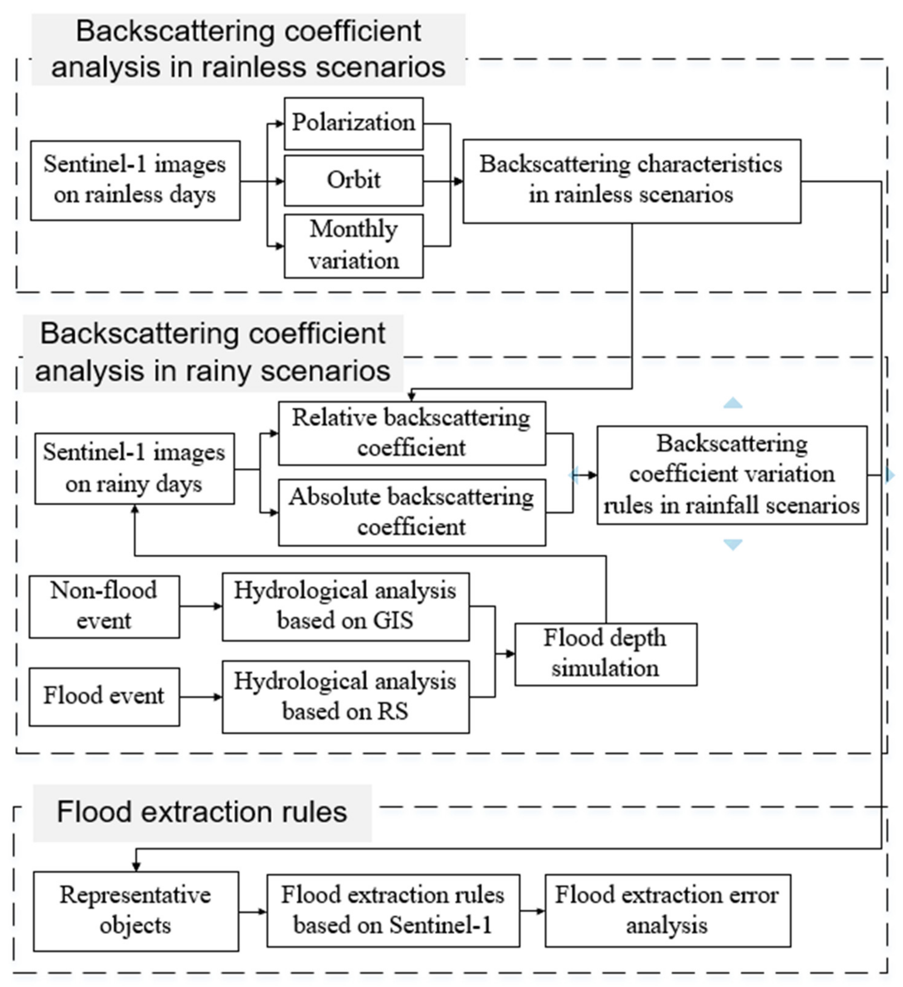
The backscattering characteristics of five ground objects in the study area were studied using multi-temporal Sentinel-1 images. The monthly variation of backscattering coefficients in rainless scenarios and the influence of polarization on the backscattering coefficients were studied to provide a basis for minimizing the error caused by seasonal variations.
Flood depth simulations were done using GIS and RS technology. The change rules of the backscattering coefficient with flood degrees in different rainfall scenarios were studied to provide an experimental basis for estimating the surface inundation state. Figure 3 shows a flow chart of this process.
2.3.1. Flood Inundation Analysis Based on GIS
The flood inundation analysis based on GIS technology has three parts: rainfall-runoff, surface rainwater conflux, and numerical simulation of surface inundation depth.
Rainfall-runoff refers to the forming net rain after deducting various losses in rainfall, i.e., mainly through evaporation, plant interception, surface depression filling, and soil infiltration. There is an obvious relationship between surface runoff and soil moisture [28]. Light rain can increase soil moisture at 0~10 cm soil depths, and moderate rain can increase it at 10–20 cm depths [29].
Surface rainwater conflux refers to the process in which runoff or floodwater flows from the surface into a pipeline network or river [30,31,32]. In our urban waterlogging simulation, the confluence of the pipe network is the link between surface water and drainage, which is the most critical part of the inundation analysis. On the other hand, rivers and ditches are the main drainage channels for rural or suburban areas without pipelines.
The numerical simulation of surface inundation depth refers to the possible surface flood depth according to the terrain after determining the total rainstorm water. The flooding algorithms based on DEM mainly include “inundation without a source” and “inundation with a source”. Inundation without a source means that the grids with lower elevation values than the given water level are inundated areas. When regional connectivity is considered, the flood can only inundate areas with flowing through [33]. As such, in this study, connectivity is not considered.
2.3.2. SCS-CN Model
The critical aspect of constructing the relationship between rainfall and surface runoff is to establish a convenient and effective rainfall-runoff model. The Soil Conservation Service Curve Number (SCS-CN) model [34,35] was developed based on the climatic characteristics and multi-year hydrological runoff data from the United States. It has been widely used due to its simple results, few parameters, and high accuracy. The SCS-CN model includes a water balance equation and two basic assumptions [36]. The balanced equation is as follows (1):
where P is rainfall (mm), Q is runoff depth (mm), F is cumulative infiltration (mm), and is initial loss (mm). Equation (2) is an assumption of equal proportions:
The assumption of a proportional relationship between the initial rainfall loss and the potential stagnant storage is described in Equation (3) [37]:
where S is the maximum infiltration of the watershed (mm), is the initial loss (mm), and is the initial loss rate.
The runoff depth can be calculated by combining Equations (1)–(3) [38,39]:
where S is calculated by the CN (Curve Number) coefficient in Equation (5) with the following statistical relationship:
Runoff CN is the model’s main parameter, which reflects the comprehensive characteristics of the soil moisture degree (Antecedent moisture condition (AMC)), slope, soil type, and land use status in the early stage of the basin. Table 1 shows the CN value of each category under the average soil humidity (AMC II) [40]. The greater the CN value is, the worse the maximum water storage capacity of the basin is.
2.3.3. Three-Level Catchment Division Method
A catchment is an area where water accumulates due to the natural landscape. It is essential to do catchment division based on ground object characteristics, because ground objects are complex and show different characteristics in rainfall-runoff processes. Catchment division methods can be categorized as either hydrologic and geometric methods. For hydrologic methods, catchments are divided with hydrological tools based on DEM. The D8 algorithm is the most widely used method [41]. However, it has poor applicability in plain areas [42,43]. For geometric methods, the nodes are determined according to research objectives, and then catchments are divided with Voronoi (Thiessen polygon) method based on nodes [44]. Voronoi diagrams are based on a set of nodes and define one area for each node with every point within the area being closer to the originating node than any other node. This method highlights the role of nodes. It ignores terrain factors and is suitable for urban areas with complex pipeline networks.
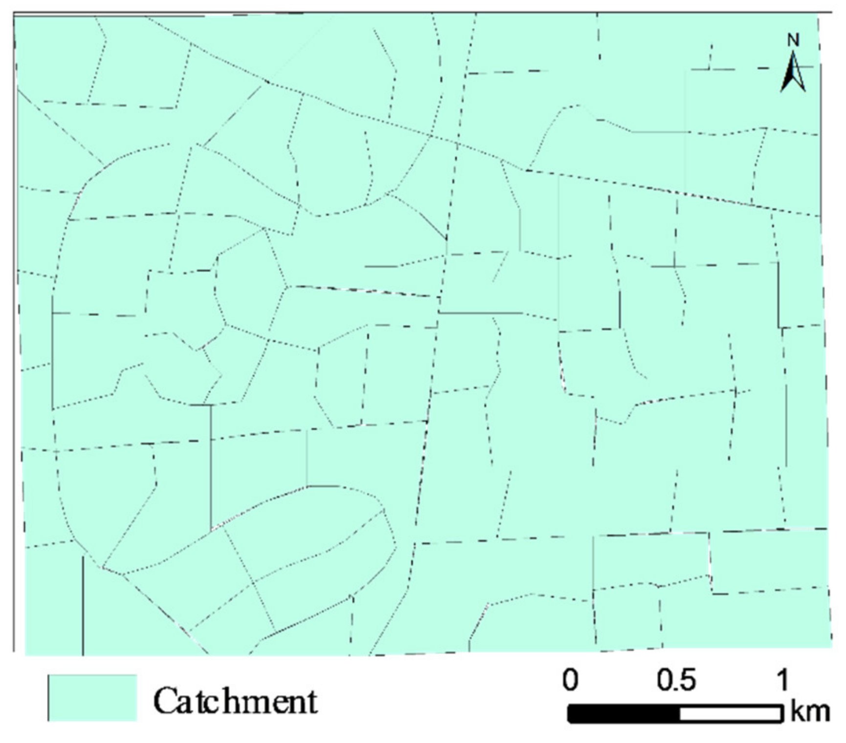
Because the study area is rural, with flat terrain and without pipelines, a three-level catchment division method using hydrologic and geometric methods was proposed to divide catchments. First, a large-scale watershed division of the study area was carried out using river channels and main roads, because river channels are subsidence areas and usually function as watershed outlets. The main road is a highway. Its elevation is higher than the grids on both sides, and the river and the main road naturally cut off the catchment. Second, for each first-level watershed, DEM data and the D8 algorithm are used to divide the catchment area into smaller parcels. However, due to the flat terrain in the area, the accumulation of confluence resulting from the use of the D8 algorithm is small, and the water flow path is short, so the catchment area is small. Usually, in the process of surface confluence, roads will generate water flow paths and the properties of the runoff between different types of land are different greatly, which limits its circulation. Therefore, the catchment areas were merged and sorted according to the secondary roads and land types. The catchment area of the study area was divided based on the three-level catchment area division method. A total of 88 catchment areas were obtained (Figure 4), and the average area was 13.33 ha.
2.3.4. Surface Flood Diffusion Algorithm with Non-Source
In actual scenarios, floods always occur in areas with low local topographies. Floods gradually diffuse according to the Digital Elevation Model (DEM) and terrain connectivity. After calculating the basin runoff Q, based on Equation (6), the flood depth and total flood water exist in the following relationship in each catchment according to the water balance theory:
where Area is the area of one grid (m2), is the runoff of the grid I (m), n is the number of grids in the current catchment area, H is the flood elevation in the catchment (m), is the elevation of the grid j (m), and m is the number of flooded grids in the catchment.
A diffusion algorithm with non-source [45] is used to calculate flood depth. It assumes that the flood starts from the grid with the lowest elevation in the catchment and gradually diffuses to grids with higher elevations. Flood diffusion ceases when flood elevation H is lower than all non-flood grids.
2.3.5. Flood Inundation Analysis Based on RS and DEM
Flood inundation analysis combined with DEM and RS is usually used to extract inundated areas based on satellite images and then calculate the flood depth through an elevation-based hydrological analysis [21].
In this study, Sentinel-1 images and a threshold method are used to extract the completely inundated area. The modified soil adjusted vegetation index (MSAVI) difference, with an empirical threshold in [46], and the change detection and threshold method (CDAT) in [47], were used to assess the partly inundated area. MSAVI difference with an empirical threshold is first used to calculate the MSAVI differences between pre-flood and flooding periods, and then to extract the inundated area based on the MSAVI difference result and an empirical threshold. MSAVI can be calculated via Equation (7):
where NIR is the Near Infrared band and Red the red band.
The CDAT method [47] can be used to determine backscattering coefficient differences using Sentinel-1 GRD products, and then to determine the threshold for common floods via Equation (8) and the threshold for floods in vegetation via Equation (9).
where is the mean of the backscattering coefficient differences, is the standard deviation of the backscattering coefficient differences, and and are the coefficients that determine these two thresholds respectively. The empirical values of and are 1.5 and 2.5 in [47].
Because the above three methods have advantages and disadvantages, all the flood areas extracted by the three methods are merged. The three-level divided catchments in Section 2.3.3 are used for the segmentation of the larger patches.
For each inundated patch, flood elevation is calculated via Equation (10). For all grids in the same inundated patch with an elevation lower than the flood elevation, flood depth is calculated via Equation (11) [21].
where is the elevation standard deviation (m) of all grids in the same inundated patch and is the elevation of grid i (m).
3. Results and Discussion
3.1. Backscattering Coefficient of Ground Objects in Rainless Scenarios
3.1.1. Selection and Statistical Analysis of Sample Points
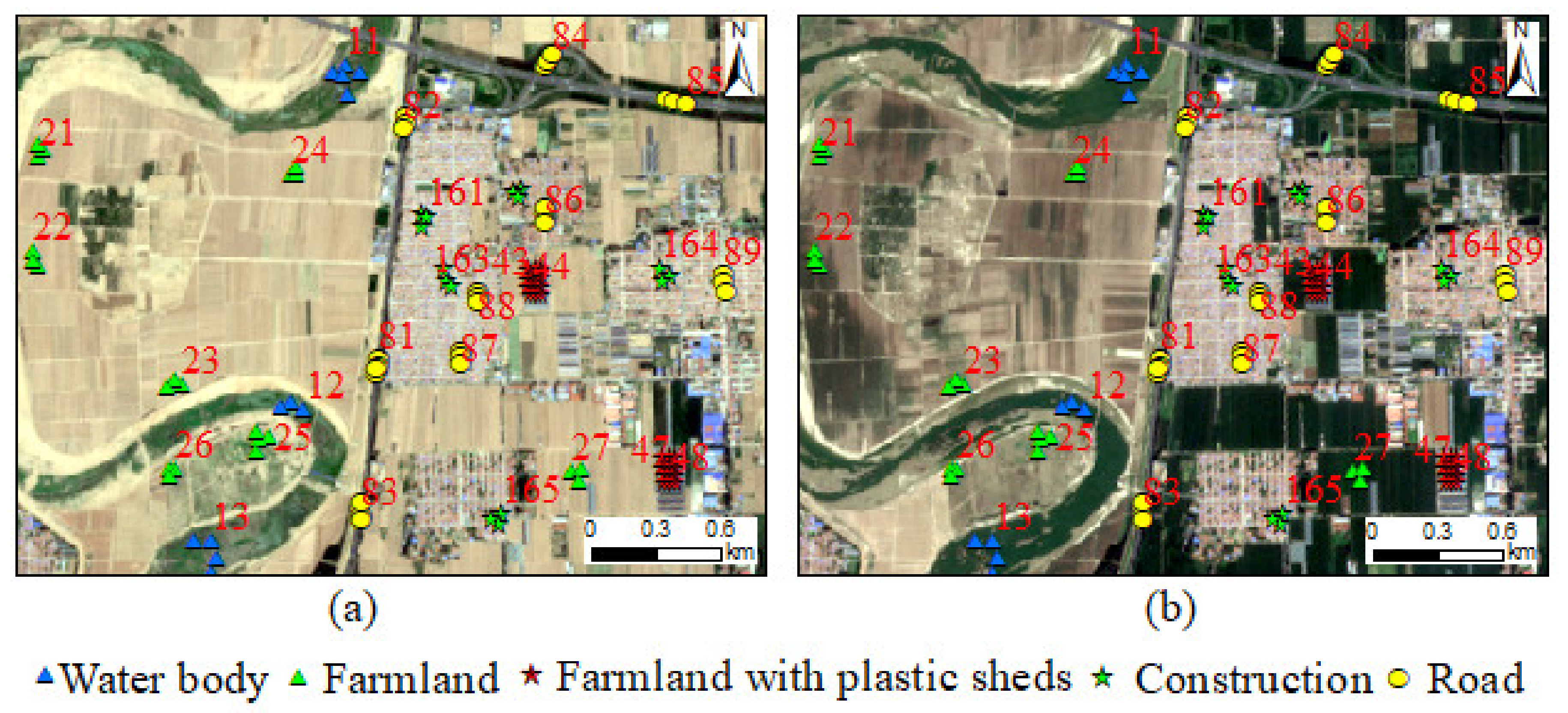
In this study, it is essential to ensure that changes are only caused by the system parameters and the ground objects themselves. Therefore, it is necessary to eliminate changes caused by artificial factors. The visual interpretation method is used to judge the changes in the study area. The test areas comprise areas that have never changed. Figure 5 shows 32 test areas with no less than 3 test areas for each ground object and no less than three points in each area. The value of each test area is the average of all points. The IDs range from 11 to 13 for water body test areas, from 21 to 27 for farmland test areas without plastic sheds, from 41 to 48 for farmland test areas with plastic sheds, from 81 to 89 for road test areas, and from 161 to 165 for construction test area.
3.1.2. Monthly Variations of Backscattering Coefficients
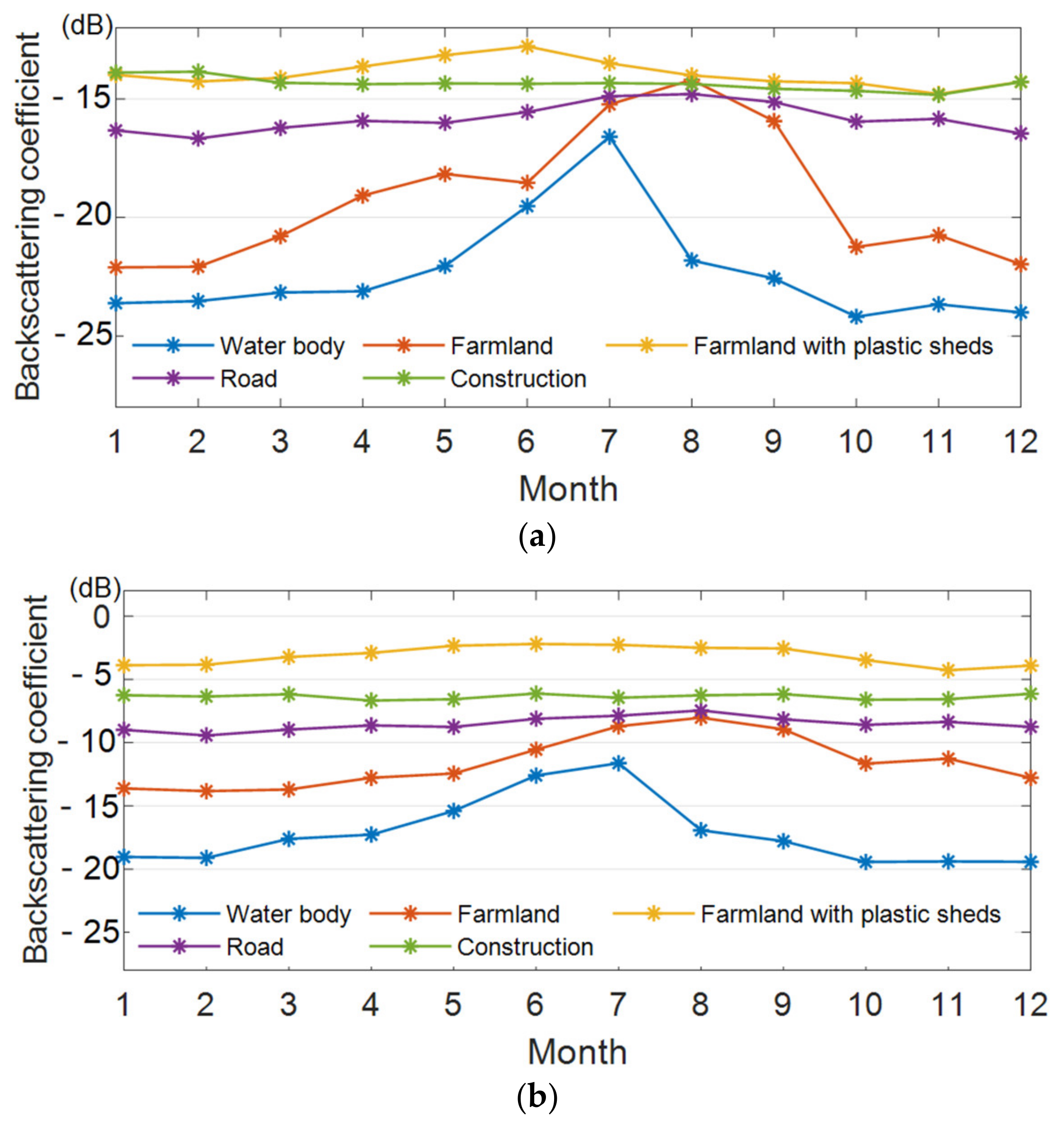
The monthly backscattering coefficients of each object are calculated based on the sample data. The backscattering coefficient with the integrated orbit is the average of the backscattering coefficients with ascending and descending orbits in the month. Table 2 shows the mean value, standard deviation, and annual maximum and minimum value of the monthly backscattering coefficient with the integrated orbit for 2019. Figure 6 shows the variations in the monthly backscattering coefficients in each category. The results show the following. (1) With VH and VV polarizations, the relationship between the annual mean backscattering coefficient of each category is as follows: water body < farmland < road< construction < farmland with plastic sheds. Road, construction, and farmland with plastic sheds present high values almost all year round. Even if the water in this study is unconventional, open water, its backscattering coefficient is the lowest each month. (2) The backscattering coefficients of road, construction, and farmland with plastic sheds vary slightly from month to month, while those of farmland and water bodies vary greatly. The standard deviations (STDs) of the backscattering coefficient of farmland with plastic sheds, road, and construction with two polarizations are all ≤0.7 dB, while that of construction with VV polarization is the smallest, i.e., only 0.2 dB. With the two polarizations, the max and min difference values between the maximum and the minimum of the three objects are only 2.1 dB and 0.6 dB, respectively. The annual change is small and stable. (3) The standard deviations of the annual backscattering coefficient of the water body and farmland are much greater than those of the other categories, i.e., both ≥1.9 dB. The annual maximum differences in the backscattering coefficient with the two polarizations are 7.6 dB and 7.8 dB, respectively. (4) The backscattering coefficient of farmland with the two polarizations reaches the maximum value in August and the minimum in January and February. The differences in the maximum value with the two polarization modes are 7.1 dB and 5.4 dB, respectively. This mainly shows an upward trend from January to July and a decreasing trend from September to December.
3.1.3. Influence of Polarization on Backscattering Coefficient
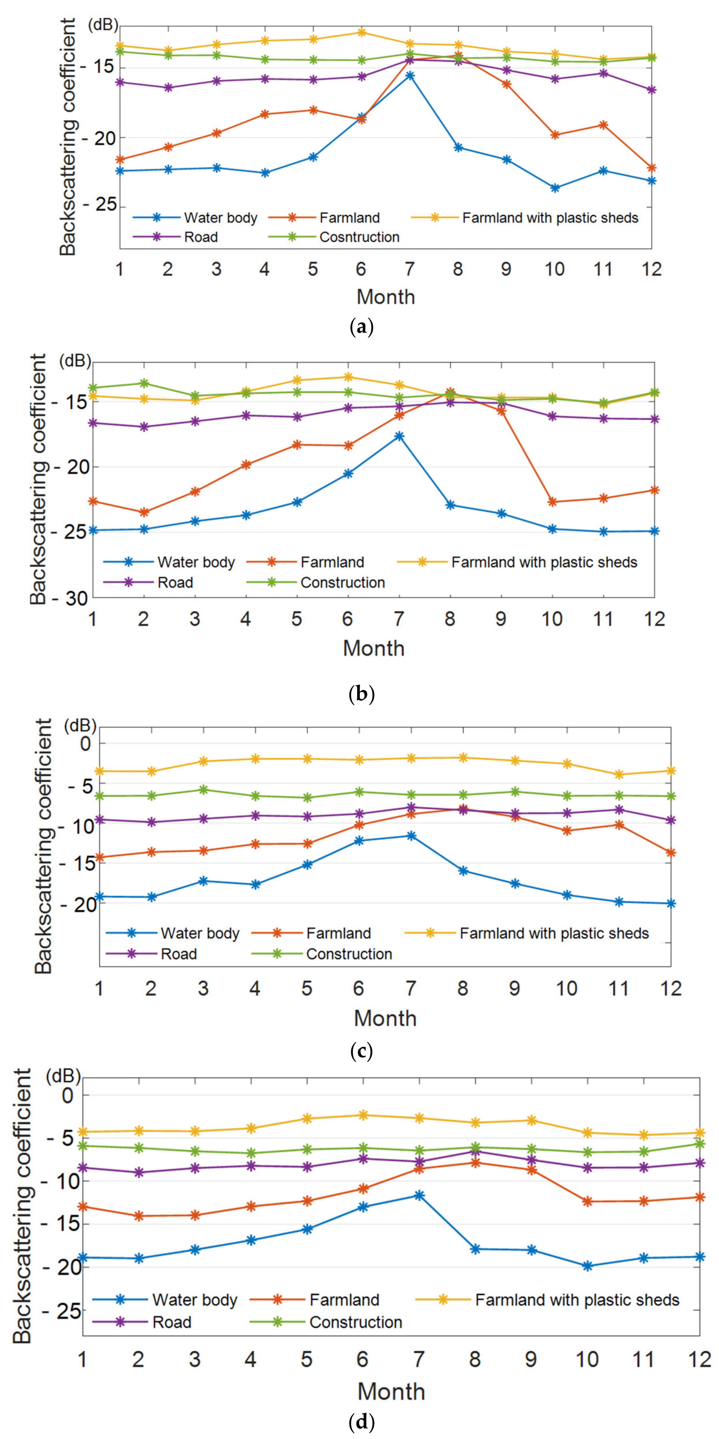
Table 3 shows the mean and standard deviation of the backscattering coefficients of each category with two polarizations in 2019. Figure 7 shows the line graph of monthly backscattering coefficient variation for each category with different polarizations and orbits.
The differences between the backscattering coefficients due to polarizations are as follows: (1) The differences of the backscattering coefficients with VH polarization are smaller than those with VV polarization. The greatest backscattering coefficient difference with two polarizations is the road, i.e., up to 10.8 dB, and water, i.e., up to 5.2 dB. (2) The maximum absolute values of the difference between the backscattering coefficient are 8.3 dB for VH and 13.9 dB for VV. (3) The annual variation with VH polarization is greater than that with VV polarization for the same category.
3.1.4. Influence of Orbit on Backscattering Coefficient
Table 4 shows the mean and standard deviation of the backscattering coefficients of each category with two orbits in 2019 and the difference in annual mean backscattering coefficients with two orbits. Combined with Table 4 and Figure 7, it reveals that the relationship between the backscattering coefficients of each category is the same. The backscattering coefficient differences of each category caused by orbit are as follows: (1) Backscattering coefficients with ascending orbits are generally greater than those with descending orbits. The max absolute value of the difference of the same category is 1.7 dB and the minimum is 0.1 dB; (2) The influence of orbit on the backscattering coefficient is less than that of polarization; and (3) The variation of the backscattering coefficient with descending orbit is greater than that with ascending orbit.
3.2. Backscattering Coefficients Change Rules of Ground Objects in Rainy Scenarios
Remote sensing images reflect the state of ground objects at the time of imaging, while SAR images reflect the backscattering characteristics of ground objects. Different rainfall leads to different flood depths, causing changes in ground object backscattering coefficients. The change in the backscattering coefficient caused by a single rainfall factor reveals the change in the water depth of ground objects. Remote sensing technology can extract flood areas but cannot measure the flood depth. As such, flood depth is simulated by hydrological analysis based on GIS and RS.
3.2.1. Flood Depth Simulation Based on the GIS and RS Techniques
Rainfall Samples
A Sentinel-1 image on a rainy day is selected as the sample, as the influence of previous rainfall should be considered when selecting samples. When the rainfall is heavy, the duration of its influence should be considered. According to previous research, large-scale surface water accumulation generally retreats completely within seven days when a single-day rainfall comprises heavy rain or lighter. The influence duration of previous rainfall may be extended according to the situation when a single-day rainfall level is a heavy rainstorm or heavier. It is currently impossible to determine the exact impact of previous rainfall. Therefore, to minimize the error caused by previous rainfall, this paper ensures that the rainfall rankings of the first 24 h, the first 72 h and the first 169 h of each event are consistent when selecting the rainfall events. Table 5 shows the five rainfall samples and presents specific rainfall information. In line with the Chinese rainfall classification standards, the four rainfall events are categorized as moderate rain, heavy rain, rainstorm, rainstorm, and heavy rainstorm.
Waterbody Extraction Based on RS Images and Threshold Method
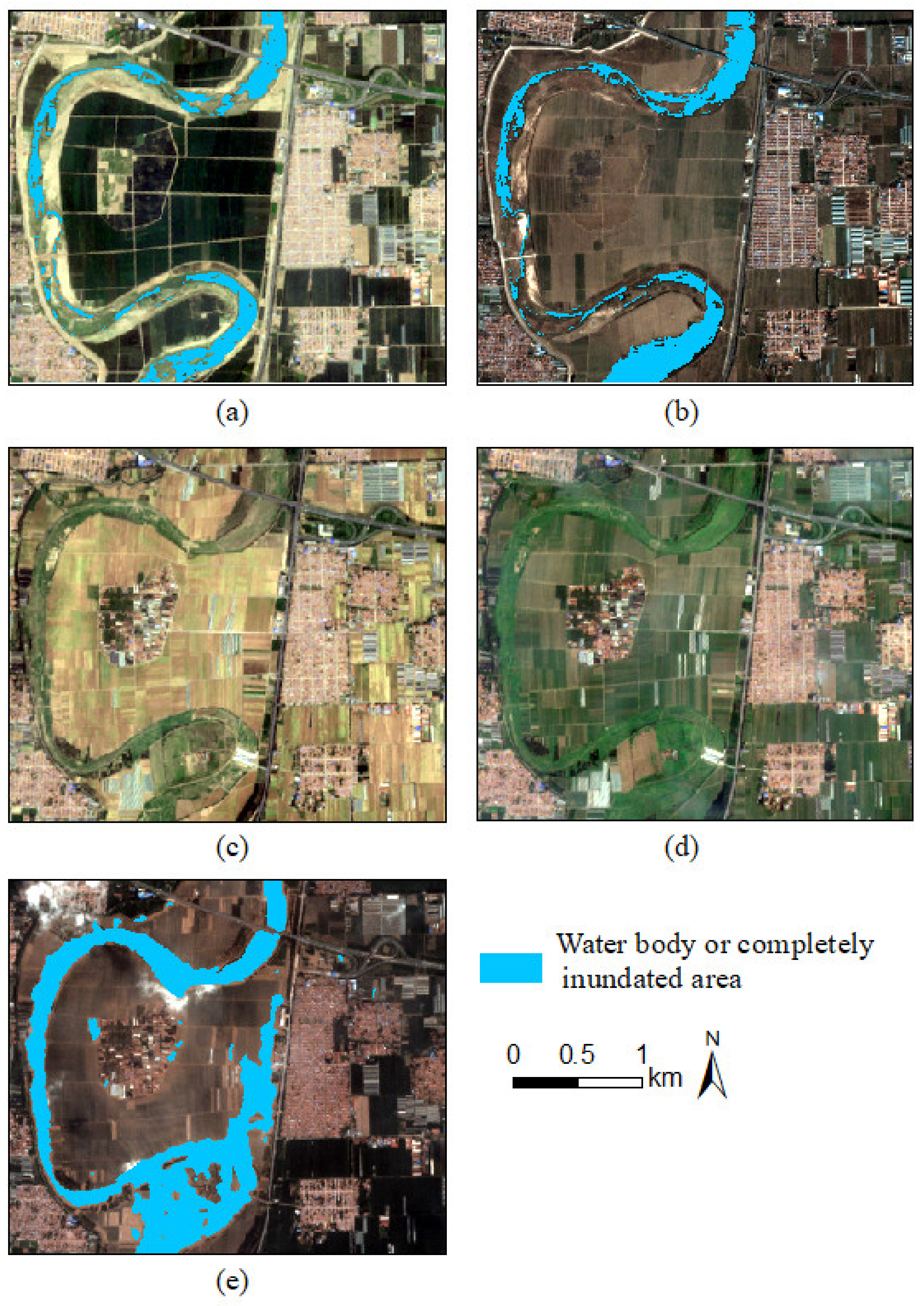
The water body was extracted with a threshold method and Sentinel-1/2 images to determine the completely inundated areas in each rainfall. The bimodal method is used to extract the range of water bodies in five rainfall events. This method requires an appropriate proportion of water area in the total image area. When the rainfall or runoff is small, the water body is not easy to discern from SAR images. More accurate water body information can be obtained through optical images. The satellite products and their dates used for water extraction in each rainfall event are shown in Table 6. Figure 8 shows the spatial distribution of water in each rainfall event. The maps on each date are Planet satellite RGB composite images.
Flood Depth Simulation
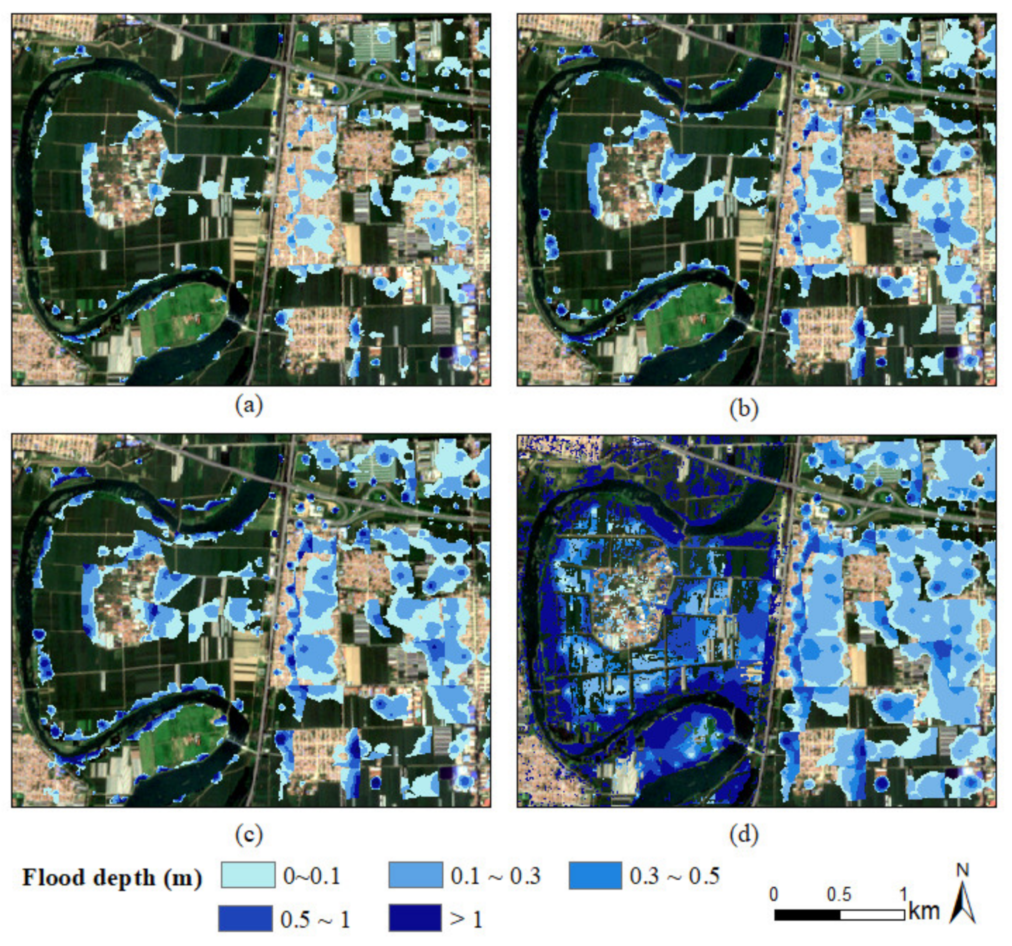
In the absence of other data support, the initial loss rate of this study area is taken as 0.2 [36]. The study area’s average CN value is about 78.92, and S is 67.84. According to the SCS-CN model, when p > 13.57 mm, the study area begins to generate surface runoff, so there was no flooding on the surface on 5 May 2020. The last four rainfalls generated runoff. Except for the rainfall on that day, the previous rainfall affected the last four rainfalls. The rainfall in the first 24–48 h of the latter two rainfalls was greater than the critical value for generating runoff. The surface runoff on 15 July 2018 was only affected by rainfall, so the total rainfall in the previous 48 h was applied. In the flood event on 20 August 2018, the flood was not only affected by rainfall but also by the overflow of the river channel. River inversion was mainly occurred in the area along the Mi River, which was the west of the main road in the study area. However, given the specific amount of river channel backflow, it was not possible to convert the incoming water into runoff using the SCS-CN model directly, and the method based on DEM and remote sensing images was used to calculate the water depth. For the whole area on 18 November 2020, 16 May 2018, and 15 July 2018, and for the area east of the main road during the flood on 20 August 2018, the SCS-CN method and the diffusion algorithm with non-source performed the calculation of flood depth. The flood depth distribution in the last four rainfall events is shown in Figure 9, in which the river channel range has been removed.
3.2.2. Selection and Statistical Analysis of Sample Points in the Context of Flood Mapping
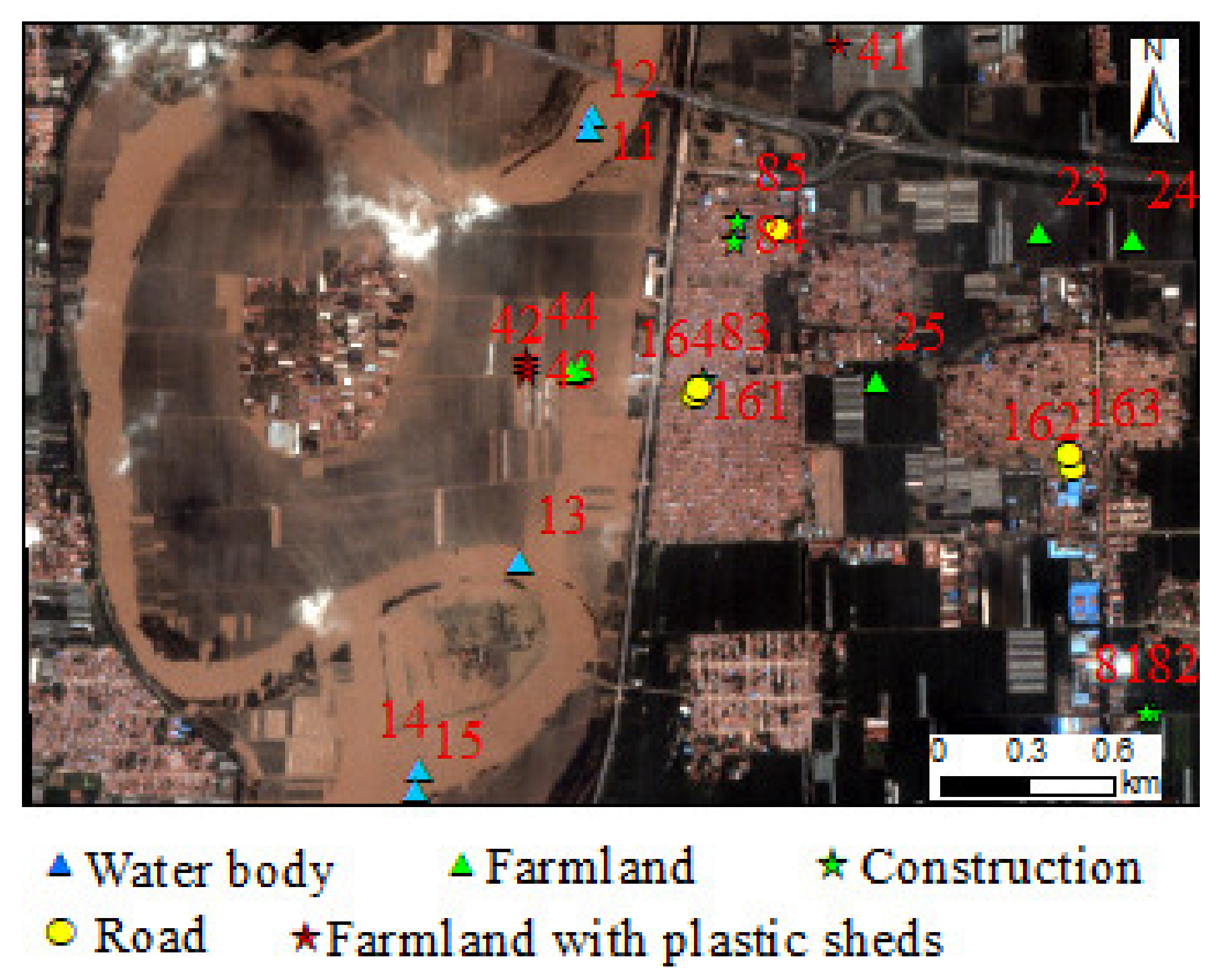
The sample points are those with obvious inundation during rainfall, based on the flood depth simulation results. Such points are usually local depressions, and flood depth continues to increase with increased rainfall. Figure 10 shows the distribution of the sample points. The IDs of water body sample points are from 11 to 15 in Mi River. In the rainfall event on 20 August 2018, the Mihe River was full and was considered an open water body. Therefore, the mean value of the backscattering coefficients of all the water sample points on this day is taken as the backscattering coefficient of an open water body, which provides a reference for studying variations in the backscattering coefficients of ground objects in different rainfall scenarios. The IDs range from 21 to 25 for farmland sample points, and points 21 and 22 were completely inundated during the last rainfall. The IDs range from 41 to 44 for farmland with plastic sheds sample points, the IDs range from 81 to 85 for road sample points, and the IDs range from 161 to 165 for construction sample points. Because of the frequent changes in farmland with plastic sheds, all areas underwent change and were flooded in the five rainfalls. As such, the experimental data of the farmland with plastic sheds were only from the three rainfall events in 2018.
Table 7 shows the flood depths of all sample points resulting from five rainfall events. There is no flood in any of the sample points during light rain, but a roughly 10-cm flood depth is occurred due to moderate rain, roughly 10- to 30 -m flood depth due to two heavy rainstorms, and more than 20-cm flood depths due to heavy rain. The flood depths of all sample points are increased with an increase in rainfall.
3.2.3. Backscattering Coefficient Change Rules for the Sample Points
The relative backscattering coefficient is the change value of each sample point relative to the corresponding monthly benchmark in each rainfall scenario. The monthly benchmark is the average of the backscattering coefficients with the integrated orbit in that month. The relative backscattering coefficient reflects the change degree in the backscattering coefficient in different rainfall scenarios or at different flood depths relative to the rainless state.
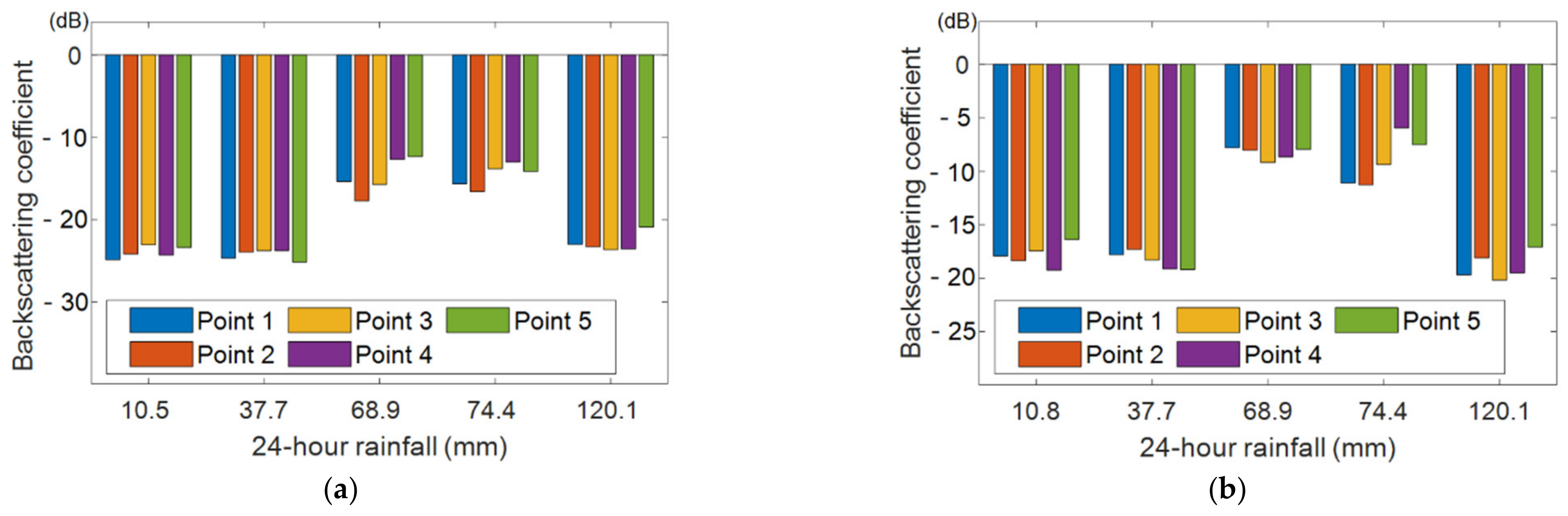
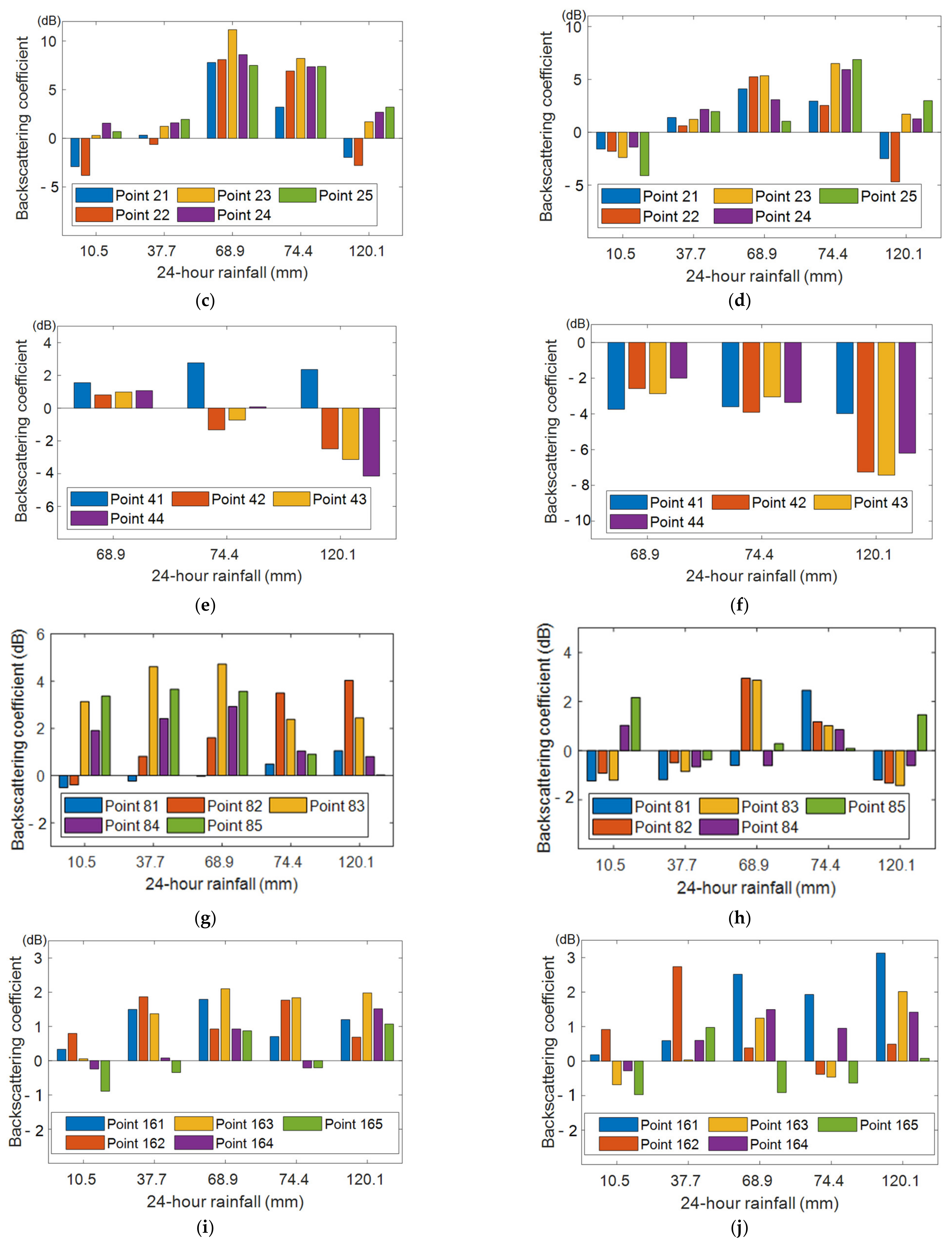
Figure 11 shows the change process for each object’s backscattering coefficient in different rainy scenarios. The results are as follows: (1) For dry or shallow rivers, the backscattering coefficients with two polarizations become smaller than the normal scattering coefficient in each rainfall scenario. (2) For the farmland, the backscattering coefficients become smaller when the soil moisture increases, but no surface runoff occurs. When the soil moisture is saturated and the flood depth does not exceed 10 cm, the backscattering coefficients for farmland are increased. The backscattering coefficients increase when the flood depths at the sample points are about 10–30 cm. When the flood depths of the sample points are greater than 30 cm, the backscattering coefficients of completely inundated sample points become smaller, while the coefficients of the incompletely inundated points increase. (3) For the farmland with plastic sheds, the flood depths are less than 15 cm due to the two rainstorms, but the change trends of the coefficients are inconsistent. During the flood, sample points from 42 to 44 are completely inundated and the flood depths are greater than 30 cm. As such, the backscattering coefficients of the sample points become smaller. The flood depth of sample point 41 is less than 20 cm, and the backscattering coefficient of this point becomes larger with VH polarization and smaller with VV polarization. Additionally, the change of backscattering coefficient amplitude is smaller than that of the sample point with a flood depth greater than 30 cm. (4) For the road, the backscattering coefficients with the two polarizations are increased with the increasing inundation. (5) During the continuous increase of flood depth in the construction site, the backscattering coefficients with the two polarizations are increased slightly. (6) A comprehensive analysis of the variation of the other four classifications, except for water, show that the variation with VH polarization is greater than that with VV polarization, and the variation of the backscattering coefficients of farmland is the largest, and the trends of construction sire and road are the same, demonstrating only relatively small changes.
The absolute backscattering coefficient is the original backscattering coefficient without other processing. This reflects the backscattering state of ground objects in different rainfall conditions, which is used to determine representative objects with different flood depths.
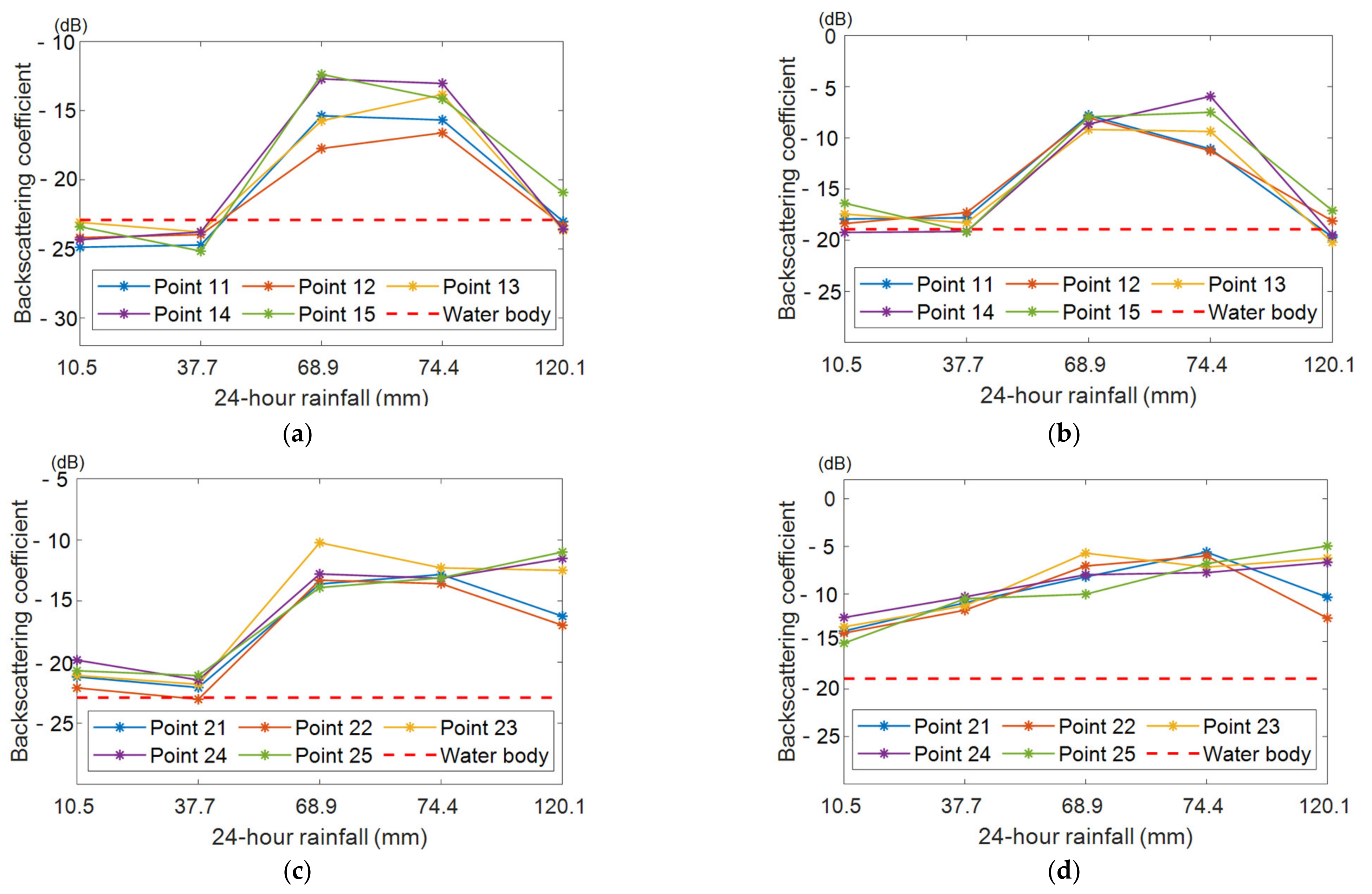
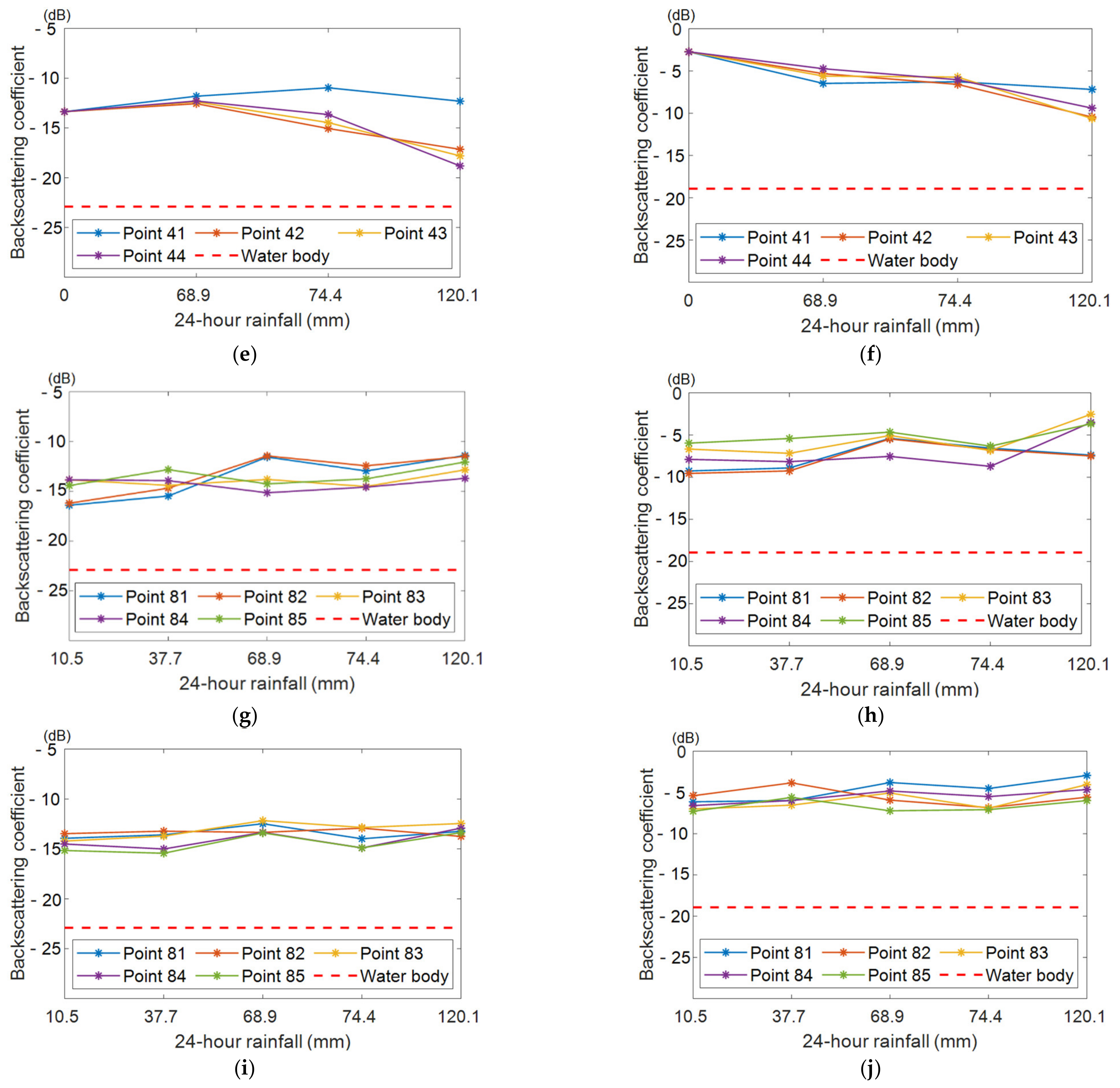
Figure 12 shows the change process of the absolute backscattering coefficients of each object in different rainfall scenarios. The main conclusions are as follows: (1) The backscattering coefficient experienced a process of first increasing and then decreasing for the water body. In the two rainfall events, the Mi River runoff demonstrated little difference and the scattering coefficient did not change significantly. Following the heavy rain, the Mi River changed from the original underflow, but the runoff rating is changed to no obvious runoff. Additionally, the absolute scattering coefficients are increased sharply with both polarizations. Through experiments, it is found that the river runoff in this area is greatly affected by human activity and is not consistent with rainfall. However, it is also found that the relevant backscattering coefficient is greatly reduced when the flow is full. (2) For farmland, when the flood depth is less than 30 cm, all the sample points show the same backscattering coefficient variation rules. When the flood depth is less than 10 cm, the backscattering coefficient is decreased slightly with VH polarization and increased with VV polarization. Following an increase in the flood depth to 30 cm, the backscattering coefficients are increased with both polarizations. When the flood depth is greater than 30 cm but complete inundation has not occurred, the backscattering coefficient of the various points is increased. The backscattering coefficient of the completely inundated points is decreased. (3) For the farmland with plastic sheds, the absolute backscattering coefficient is unchanged when the flood depth is less than 20 cm and not completely inundated. In the completely inundated state, the flood depth is greater than 30 cm and the backscattering coefficients with both polarizations become smaller. (4) Road and construction settings generally show a slight upward trend with increasing flood depth.
3.3. Flood Extraction Rules Based on Sentinel-1
3.3.1. Selection of Representative Objects of Flood State
Representative objects of flood state comprise ground objects for representing the backscattering state of different objects and their different inundated states. The backscattering characteristics of all representative objects are taken from their status in a rainless scenario. Representative objects are determined by the backscattering coefficient change rules of ground objects in different inundated states. The backscattering coefficients of five ground objects in different inundated states are within the range of those in rainless scenarios. Thus, the backscattering coefficients of five ground objects in rainless scenarios can represent different inundated states.
Taking backscattering coefficients with VH polarization and descending orbit as an example, the backscattering coefficients of five ground objects range from −24.0 to 14.0 dB. The backscattering coefficients variation of road, farmland with plastic sheds, and construction are small, centering around −16.0 to −14.0 dB. As such, the three objects are not subdivided. The backscattering coefficient of the water body is −23.3 dB, and the annual average backscattering coefficient of farmland is −19.8 dB. If the annual average backscattering coefficient of the farmland is used as a representative object, there is no representative object to cover backscattering coefficients around −19.0 to −16.0 dB. The backscattering coefficient variation of farmland is large. To more accurately represent the inundation state of ground objects and reveal the small coefficient differences, the backscattering characteristics of farmland are further subdivided. Combined with the backscattering coefficients of farmland in different inundation depths, the coefficients are subdivided into farmland with low (January), with medium (May), and with high backscattering (August). In summary, the final objects with representing the backscattering characteristic state of ground objects are as follows: water body, farmland with low backscattering, farmland with medium backscattering, farmland with high backscattering, road, construction, and farmland with plastic sheds.
3.3.2. Flood Degree Estimation Rules of Ground Objects Based on Sentinel-1 Images
According to the relative and absolute change of backscattering coefficients of objects in different rainfall scenarios, combined with the estimation results of flood depths at the sample points, the rules for judging the inundation degree of ground objects based on Sentinel-1 images are determined. The backscattering coefficient of the water body with two polarizations becomes smaller with each rainfall. In the full flow state it is very low, while under the semi-dry state it is close to those of the construction and farmland with plastic sheds. The backscattering of farmland increases with the increasing flood depth, and the backscattering coefficient in the completely inundated state is close to that of the water body. The backscattering coefficient with the two polarizations becomes smaller when the farmland with plastic sheds is completely inundated and the inundation depth is greater than 30 cm. Before complete inundation, the variation of the absolute backscattering coefficient is small and the relative backscattering coefficient with two polarizations is inconsistent, so the flood degree cannot be determined according to the variation rule of the backscattering coefficient. The backscattering coefficients of road and construction show a slight upward trend.
Combined with the results of representative object selection and the ground object backscattering coefficient variation with different flood depths, the flood degree estimation rules for ground objects based on Sentinel-1 can be determined. A mildly inundated state means that the flood begins to appear on the surface and the flood depth is less than 10 cm. A moderately inundated state means the flood depth is more than 10 cm and less than 30 cm. A completely inundated state means that the ground object is completely inundated and the scattering coefficient presents an open water state independent of the inundated depth. All the ground objects are completely inundated when their backscattering coefficients are close to that of open water. The backscattering coefficient of farmland with medium and high backscattering in a mildly inundated state is close to those of construction and farmland with plastic sheds. The backscattering coefficient of farmland with medium backscattering in a moderately inundated state is close to those of road and farmland with high backscattering. The backscattering coefficient of farmland with high backscattering in a moderately inundated state is close to that of road and farmland with medium backscattering. The backscattering coefficient of the road in a mildly inundated state is close to those of construction and farmland with plastic sheds when the latter is moderately inundated. The backscattering coefficient of construction in a mildly inundated state is close to that of farmland with plastic sheds.
3.3.3. Flood Extraction Error Caused by Monthly Object Variation and Orbit Differences
The key to flood extractions based on SAR images is change detection of backscattering coefficients in the pre-flood and post-flood periods. Especially when the flood extraction is done based on change detection and the threshold method using original backscattering coefficient differences between pre-flood and post-flood periods [35], coefficient differences have an important influence on the flood extraction results. According to the above-mentioned research results, monthly variation and orbits, in addition to floods, can cause backscattering coefficient differences. Therefore, flood extraction errors caused by monthly variation and orbits can be quantitatively estimated by comparing them with the backscattering coefficient differences caused by the flood.
Table 8 shows the details of the backscattering coefficient differences due to flood, monthly variation and orbit. When the coefficient differences between monthly coefficients and the maximum of that caused by orbits are larger than the minimum coefficient differences caused by flooding, monthly variation and orbit may cause extraction errors. The following can be concluded by comparing the data in the third, fourth, and fifth columns: (1) The monthly backscattering coefficient variation affects flood extractions of farmland, road, and construction with VH and VV polarization. In particular, the maximum difference of monthly backscattering coefficients of farmland is much greater than that between different inundation states. (2) The backscattering coefficient differences caused by the orbit mainly affect the flood extraction results of farmland and road with VH polarization. (3) The influence of monthly variation of the backscattering coefficient on flood extraction results is greater than that of the orbit.
3.3.4. Pre-Flood Reference Image Selection Rules
It is vital to select a reasonable pre-flood reference image, especially when the flood methods directly use the backscattering coefficients in the pre-flood and flooding period [47]. The pre-flood reference image is determined according to the selected image parameters in the flooding period. Because light rain (<10 mm) can be completely absorbed by surface soil (0~10 cm), its influence on the surface is relatively small, while the influence of heavier rainfall is uncertain. Additionally, while floods often occur in the rainy season, it may be difficult to find a reference image without any previous rainfall. Section 3.3.3 shows that monthly variation and orbit may cause flood extraction errors. Therefore, pre-flood reference images must meet the following three conditions: (1) no daily rainfall is greater than 10 mm within one week before the flood; (2) The orbit parameters are consistent with the images in the flooding period; and (3) The imaging time of the reference image and the flooding period should not differ by more than one month.
3.4. Discussion
Multi-temporal image analysis and flood depth simulation based on GIS and hydrological analysis are conducted to study the monthly variation of backscattering coefficients in rainless scenarios and the change rules of backscattering coefficients according to flood depths. The influence of orbit on backscattering coefficient and improvements for flood extraction rules, i.e., by transitioning from qualitative to semi-quantitative analyses, are presented. However, due to the lack of measured data or limited current technical means, this study still has some shortcomings: (1) While soil moisture is the dominant factor in soil dielectric properties, radar imaging is also affected by soil moisture. However, due to the lack of measured soil moisture data, relevant experiments cannot be carried out. Therefore, the influence of soil moisture on backscattering coefficients should be further studied. The groundwater level in the study area changed greatly around 2018, which led to a large difference in soil moisture contents in different years. Only Sentinel-1 data from 2019 were used to reduce the errors caused by soil moisture, which should be further discussed. (2) There is currently no effective method for observing flood depth based on remote sensing images. The flood depth simulation method used in this paper can estimate the relative degree of a flood. According to the degree of change of the backscattering coefficient, it can judge whether it has changed. However, when the change is small, it is impossible to judge whether the backscattering coefficient is insensitive to the flood degree or whether the ground objects themselves have not changed. A more accurate method should be investigated to improve evaluations of flood degree in the future.
4. Conclusions
This paper aimed to improve the accuracy of flood mapping using Sentinel-1 images by analyzing backscatter characteristics, including supplementing prior knowledge of flood extraction and quantitatively evaluating flood extraction errors due to non-rainfall factors. For the influence of non-flood factors on backscattering coefficients, the monthly variation of the backscattering coefficients of ground objects with different polarizations and orbits was studied using multi-temporal Sentinel-1 images in rainless scenarios. Variations of backscattering coefficients with different flood depths were studied using Sentinel-1 data showing different degrees of rainfall. A hydrological analysis based on GIS and RS was used to simulate flood depths. The results showed that the monthly variations of the maximum backscattering coefficients of farmland and construction and the backscattering coefficient differences caused by the satellite orbit were larger than the minimum backscattering coefficient differences caused by inundation. The flood extraction rules of five objects based on Sentinel-1 are obtained. The main conclusions and contributions are summarized as follow: (1) Flood extraction rules based on Sentinel-1 images were obtained, which improves the flood extraction rules from qualitative to semi-quantitative analyses. (2) The flood extraction error was quantitatively analyzed and evaluated by comparing backscattering coefficient differences caused by monthly variation, polarization, and orbit to that caused by the flood. This provides a reference for selecting pre-flood images or appropriate flood extraction methods.
Author Contributions
Conceptualization, M.H. and S.J.; methodology, M.H. and S.J.; software, M.H.; validation, M.H. and S.J.; formal analysis, M.H.; investigation, M.H.; resources, M.H. and S.J.; data curation, M.H.; writing—original draft preparation, M.H. and S.J.; writing—review and editing, S.J.; visualization, M.H.; supervision, S.J.; project administration, S.J.; funding acquisition, S.J. All authors have read and agreed to the published version of the manuscript.
Funding
The work was supported by the Strategic Priority Research Program Project of the Chinese Academy of Sciences, grant number XDA23040100, and Jiangsu Natural Resources Development Special Project, grant number JSZRHYKJ202002.
Institutional Review Board Statement
Not applicable.
Informed Consent Statement
Not applicable.
Data Availability Statement
The rainfall data were available from the website of the China Meteorological Data Service Center (http://data.cma.cn).
Acknowledgments
The authors thanks ESA for providing Sentinel-1/2 data and Planet Labs for providing Planet images.
Conflicts of Interest
The authors declare no conflict of interest.
References
- Borah, S.B.; Sivasankar, T.; Ramya, M.N.S.; Raju, P.L.N. Flood inundation mapping and monitoring in Kaziranga National Park, Assam using Sentinel-1 SAR data. Environ. Monit. Assess. 2018, 190, 520. [Google Scholar] [CrossRef] [PubMed]
- Grimaldi, S.; Xu, J.; Li, Y.; Pauwels, V.; Walker, J. Flood mapping under vegetation using single SAR acquisitions. Remote Sens. Environ. 2020, 237, 111582. [Google Scholar] [CrossRef]
- Zhang, Y.-P.; Jiang, L.-M.; Qiu, Y.-B.; Wu, S.-L.; Shi, J.-C.; Zhang, L.-X. Study of the microwave emissivity characteristics over different land cover types. Spectrosc. Spectr. Anal. 2010, 30, 1446–1451. [Google Scholar]
- Guccione, P.; Lombardi, A.; Giordano, R. Assessment of seasonal variations of radar backscattering coefficient using sentinel-1 data. In Proceedings of the 2016 IEEE International Geoscience and Remote Sensing Symposium (IGARSS), Beijing, China, 10–15 July 2016; pp. 3402–3405. [Google Scholar] [CrossRef]
- Schlaffer, S.; Chini, M.; Giustarini, L.; Matgen, P. Probabilistic mapping of flood-induced backscatter changes in SAR time series. Int. J. Appl. Earth Obs. Geoinf. 2017, 56, 77–87. [Google Scholar] [CrossRef]
- Zhang, M.; Li, Z.; Tian, B.; Zhou, J.; Tang, P. The backscattering characteristics of wetland vegetation and water-level changes detection using multi-mode SAR: A case study. Int. J. Appl. Earth Obs. Geoinf. 2016, 45, 1–13. [Google Scholar] [CrossRef]
- Zhou, L. Extraction of Planting Structure and Analysis of Spatial-Temporal Distribution Characteristics in Irrigated Areas Based on Sentinel Data. Master’s Thesis, Anhui University of Science and Technology, Huainan, China, 10 June 2019. [Google Scholar]
- Pierdicca, N.; Pulvirenti, L.; Boni, G.; Squicciarino, G.; Chini, M. Mapping Flooded Vegetation Using COSMO-SkyMed: Comparison With Polarimetric and Optical Data Over Rice Fields. IEEE J. Sel. Top. Appl. Earth Obs. Remote Sens. 2017, 10, 2650–2662. [Google Scholar] [CrossRef]
- Schlaffer, S.; Matgen, P.; Hollaus, M.; Wagner, W. Flood detection from multi-temporal SAR data using harmonic analysis and change detection. Int. J. Appl. Earth Obs. Geoinf. 2015, 38, 15–24. [Google Scholar] [CrossRef]
- Li, Y.; Martinis, S.; Wieland, M. Urban flood mapping with an active self-learning convolutional neural network based on TerraSAR-X intensity and interferometric coherence. ISPRS J. Photogramm. Remote Sens. 2019, 152, 178–191. [Google Scholar] [CrossRef]
- Martinis, S.; Rieke, C. Backscatter Analysis Using Multi-Temporal and Multi-Frequency SAR Data in the Context of Flood Mapping at River Saale, Germany. Remote Sens. 2015, 7, 7732–7752. [Google Scholar] [CrossRef] [Green Version]
- Sun, Y.; Huang, S.; Li, J.; Ling, X.; Ma, J.; Qu, W. The Downstream flood monitoring application of Myanmar Irrawaddy River based on Sentinel-1A SAR. Remote Sens. Technol. Appl. 2017, 32, 282–288. [Google Scholar] [CrossRef]
- Hess, L.L.; Melack, J.M. Remote sensing of vegetation and flooding on Magela Creek Floodplain (Northern Territory, Australia) with the SIR-C synthetic aperture radar. Hydrobiologia 2003, 500, 65–82. [Google Scholar] [CrossRef]
- Voormansik, K.; Praks, J.; Antropov, O.; Jagomagi, J.; Zalite, K. Flood Mapping With TerraSAR-X in Forested Regions in Estonia. IEEE J. Sel. Top. Appl. Earth Obs. Remote Sens. 2014, 7, 562–577. [Google Scholar] [CrossRef]
- Pulvirenti, L.; Pierdicca, N.; Chini, M.; Guerriero, L. Monitoring Flood Evolution in Vegetated Areas Using COSMO-SkyMed Data: The Tuscany 2009 Case Study. IEEE J. Sel. Top. Appl. Earth Obs. Remote Sens. 2013, 6, 1807–1816. [Google Scholar] [CrossRef]
- Kundu, S.; Aggarwal, S.P.; Kingma, N.C.; Mondal, A.; Khare, D. Flood monitoring using microwave remote sensing in a part of Nuna river basin, Odisha, India. Nat. Hazards 2015, 76, 123–138. [Google Scholar] [CrossRef]
- Richards, J.A.; Woodgate, P.W.; Skidmore, A.K. An explanation of enhanced radar backscattering from flooded forests. Int. J. Remote Sens. 1987, 8, 1093–1100. [Google Scholar] [CrossRef]
- Bhogapurapu, N.; Dey, S.; Bhattacharya, A.; Mandal, D.; Lopez-Sanchez, J.M.; McNairn, H.; López-Martínez, C.; Rao, Y. Dual-polarimetric descriptors from Sentinel-1 GRD SAR data for crop growth assessment. ISPRS J. Photogramm. Remote Sens. 2021, 178, 20–35. [Google Scholar] [CrossRef]
- Ezzine, A.; Darragi, F.; Rajhi, H.; Ghatassi, A. Evaluation of Sentinel-1 data for flood mapping in the upstream of Sidi Salem dam (Northern Tunisia). Arab. J. Geosci. 2018, 11, 170. [Google Scholar] [CrossRef]
- Zhang, B.; Wdowinski, S.; Gann, D.; Hong, S.-H.; Sah, J. Spatiotemporal variations of wetland backscatter: The role of water depth and vegetation characteristics in Sentinel-1 dual-polarization SAR observations. Remote Sens. Environ. 2022, 270, 112864. [Google Scholar] [CrossRef]
- Jo, M.-J.; Osmanoglu, B.; Zhang, B.; Wdowinski, S. Flood extent mapping using dual-polarimetric sentinel-1 synthetic aperture radar imagery. In Proceedings of the ISPRS—International Archives of the Photogrammetry, Remote Sensing and Spatial Information Sciences, Beijing, China, 7–10 May 2018; Volume XLII-3. [Google Scholar] [CrossRef] [Green Version]
- Grimaldi, S.; Li, Y.; Pauwels, V.R.N.; Walker, J.P. Remote Sensing-Derived Water Extent and Level to Constrain Hydraulic Flood Forecasting Models: Opportunities and Challenges. Surv. Geophys. 2016, 37, 977–1034. [Google Scholar] [CrossRef]
- Twele, A.; Cao, W.; Plank, S.; Martinis, S. Sentinel-1-based flood mapping: A fully automated processing chain. Int. J. Remote Sens. 2016, 37, 2990–3004. [Google Scholar] [CrossRef]
- Conde, F.C.; Muñoz, M.D.M. Flood Monitoring Based on the Study of Sentinel-1 SAR Images: The Ebro River Case Study. Water 2019, 11, 2454. [Google Scholar] [CrossRef] [Green Version]
- The China Meteorological Data Service Center. Available online: http://data.cma.cn (accessed on 30 December 2020).
- Chen, C.; Zhao, N.; Yue, T.; Guo, J. A generalization of inverse distance weighting method via kernel regression and its application to surface modeling. Arab. J. Geosci. 2014, 8, 6623–6633. [Google Scholar] [CrossRef] [Green Version]
- Maleika, W. Inverse distance weighting method optimization in the process of digital terrain model creation based on data collected from a multibeam echosounder. Appl. Geomat. 2020, 12, 397–407. [Google Scholar] [CrossRef]
- Zhang, D.-H.; Li, X.-R.; Zhang, F.; Zhang, Z.-S.; Chen, Y.-L. Effects of rainfall intensity and intermittency on woody vegetation cover and deep soil moisture in dryland ecosystems. J. Hydrol. 2016, 543, 270–282. [Google Scholar] [CrossRef]
- Haiyan, D.; Haimei, W. Influence of rainfall events on soil moisture in a typical steppe of Xilingol. Phys. Chem. Earth Parts A/B/C 2021, 121, 102964. [Google Scholar] [CrossRef]
- Babaei, S.; Ghazavi, R.; Erfanian, M. Urban flood simulation and prioritization of critical urban sub-catchments using SWMM model and PROMETHEE II approach. Phys. Chem. Earth Parts A/B/C 2018, 105, 3–11. [Google Scholar] [CrossRef]
- Ma, B.; Wu, Z.; Hu, C.; Wang, H.; Xu, H.; Yan, D.; Soomro, S.-E. Process-oriented SWMM real-time correction and urban flood dynamic simulation. J. Hydrol. 2022, 605, 127269. [Google Scholar] [CrossRef]
- Yazdi, M.N.; Ketabchy, M.; Sample, D.J.; Scott, D.; Liao, H. An evaluation of HSPF and SWMM for simulating streamflow regimes in an urban watershed. Environ. Model. Softw. 2019, 118, 211–225. [Google Scholar] [CrossRef]
- Liang, J.; Liu, D. A local thresholding approach to flood water delineation using Sentinel-1 SAR imagery. ISPRS J. Photogramm. Remote Sens. 2020, 159, 53–62. [Google Scholar] [CrossRef]
- Shi, W.; Huang, M.; Gongadze, E.; Wu, L. A Modified SCS-CN Method Incorporating Storm Duration and Antecedent Soil Moisture Estimation for Runoff Prediction. Water Resour. Manag. 2017, 31, 1713–1727. [Google Scholar] [CrossRef]
- Khzr, B.O.; Ibrahim, G.R.F.; Hamid, A.A.; Ail, S.A. Runoff estimation using SCS-CN and GIS techniques in the Sulaymaniyah sub-basin of the Kurdistan region of Iraq. Environ. Dev. Sustain. 2022, 24, 2640–2655. [Google Scholar] [CrossRef]
- Shi, Z.-H.; Chen, L.-D.; Fang, N.-F.; Qin, D.-F.; Cai, C.-F. Research on the SCS-CN initial abstraction ratio using rainfall-runoff event analysis in the Three Gorges Area, China. Catena 2009, 77, 1–7. [Google Scholar] [CrossRef]
- Walega, A.; Amatya, D.M.; Caldwell, P.; Marion, D.; Panda, S. Assessment of storm direct runoff and peak flow rates using improved SCS-CN models for selected forested watersheds in the Southeastern United States. J. Hydrol. Reg. Stud. 2020, 27, 100645. [Google Scholar] [CrossRef]
- Walega, A.; Salata, T. Influence of land cover data sources on estimation of direct runoff according to SCS-CN and modified SME methods. Catena 2019, 172, 232–242. [Google Scholar] [CrossRef]
- Liu, W.; Feng, Q.; Wang, R.; Chen, W. Effects of initial abstraction ratios in SCS-CN method on runoff prediction of green roofs in a semi-arid region. Urban For. Urban Green. 2021, 65, 127331. [Google Scholar] [CrossRef]
- Kumar, A.; Kanga, S.; Taloor, A.K.; Singh, S.K.; Đurin, B. Surface runoff estimation of Sind river basin using integrated SCS-CN and GIS techniques. HydroResearch 2021, 4, 61–74. [Google Scholar] [CrossRef]
- Costa-Cabral, M.C.; Burges, S.J. Digital Elevation Model Networks (DEMON): A model of flow over hillslopes for computation of contributing and dispersal areas. Water Resour. Res. 1994, 30, 1681–1692. [Google Scholar] [CrossRef]
- Ariza-Villaverde, A.B.; Jimenez-Hornero, F.J.; de Ravé, E.G. Influence of DEM resolution on drainage network extraction: A multifractal analysis. Geomorphology 2015, 241, 243–254. [Google Scholar] [CrossRef]
- Li, J.; Li, T.; Zhang, L.; Sivakumar, B.; Fu, X.; Huang, Y.; Bai, R. A D8-compatible high-efficient channel head recognition method. Environ. Model. Softw. 2020, 125, 104624. [Google Scholar] [CrossRef]
- Guth, N.; Klingel, P. Demand Allocation in Water Distribution Network Modelling—A GIS-Based Approach Using Voronoi Diagrams with Constraints. In Application of Geographic Information Systems; Alam, B.M., Ed.; IntechOpen: London, UK, 2012. [Google Scholar] [CrossRef] [Green Version]
- Huang, M.; Jin, S. A methodology for simple 2-D inundation analysis in urban area using SWMM and GIS. Nat. Hazards 2019, 97, 15–43. [Google Scholar] [CrossRef]
- Bi, J.; Huang, H.; Liu, Y. Flood Trace Extraction and Flood Inundation Estimation Using Remote Sensing and GIS. Remote Sens. Inf. 2016, 31, 147–152. [Google Scholar] [CrossRef]
- Long, S.; Fatoyinbo, T.; Policelli, F. Flood extent mapping for Namibia using change detection and thresholding with SAR. Environ. Res. Lett. 2014, 9, 035002. [Google Scholar] [CrossRef]
Figure 1.
Map of the study area: (a) Municipal administrative boundary of Shandong Province; (b) Sentinel-2 RGB composite image of study area of Shouguang City; (c) Planet RGB composite image of the study area.
Figure 1.
Map of the study area: (a) Municipal administrative boundary of Shandong Province; (b) Sentinel-2 RGB composite image of study area of Shouguang City; (c) Planet RGB composite image of the study area.

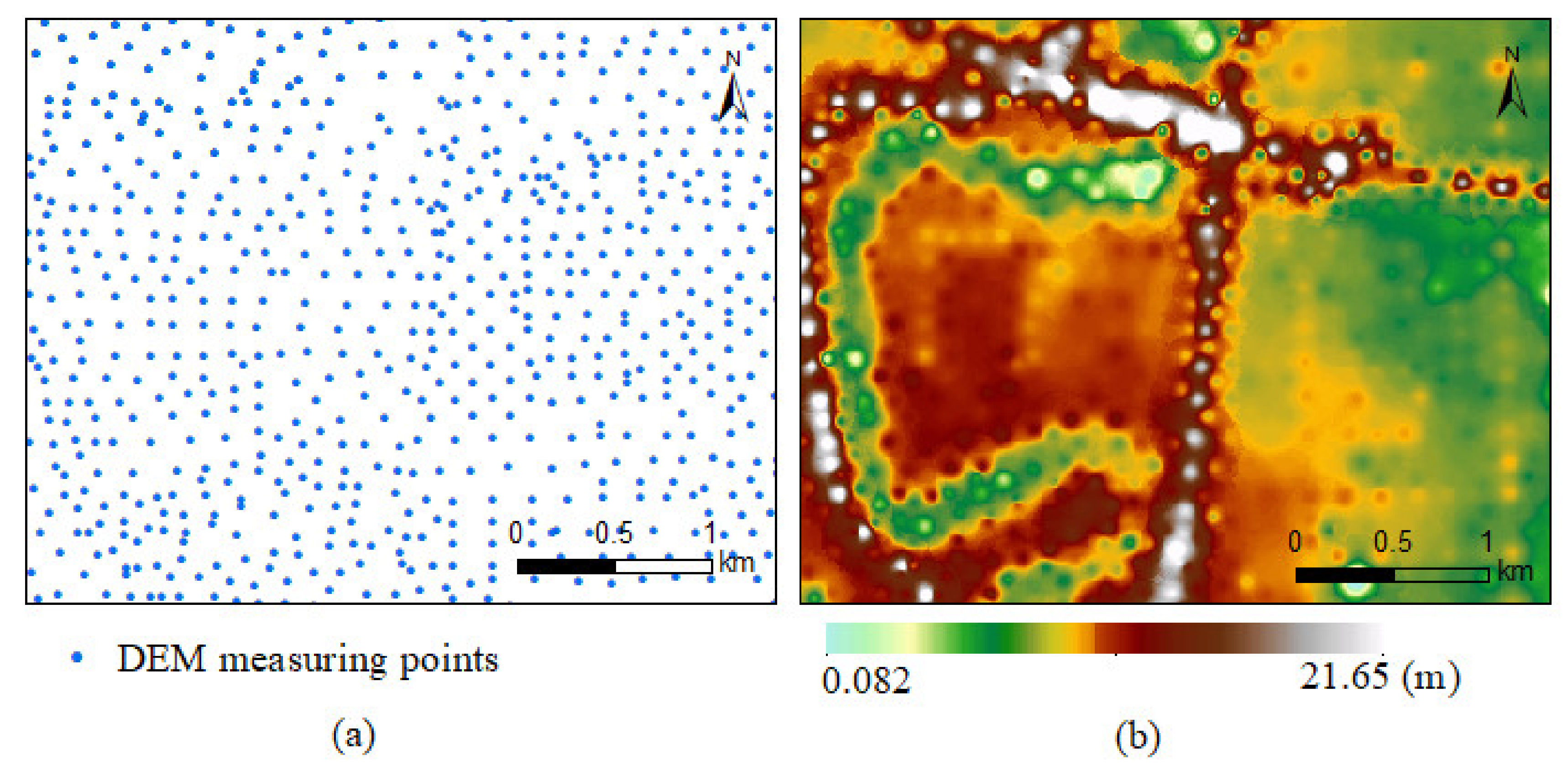
Figure 2.
DEM measuring points (a) and DEM with 10-m spatial resolution (b).

Figure 3.
Flow chart of this study.

Figure 4.
Catchment division results.

Figure 5.
Sample points in rainless scenarios: (a) the base map was a Planet RGB composite image on 26 June 2019; (b) the base map was a Planet RGB composite image on 26 June 2019.
Figure 5.
Sample points in rainless scenarios: (a) the base map was a Planet RGB composite image on 26 June 2019; (b) the base map was a Planet RGB composite image on 26 June 2019.

Figure 6.
Line chart of monthly backscattering coefficient in 2019: (a) Backscattering coefficients with integrated orbit and VH polarization; (b) Backscattering coefficients with integrated orbit and VV polarization.
Figure 6.
Line chart of monthly backscattering coefficient in 2019: (a) Backscattering coefficients with integrated orbit and VH polarization; (b) Backscattering coefficients with integrated orbit and VV polarization.

Figure 7.
Monthly backscattering coefficients with different polarizations and orbits: (a) VH and ascending orbit; (b) VH and descending orbit; (c) VV and ascending orbit; (d) VV and descending orbit.
Figure 7.
Monthly backscattering coefficients with different polarizations and orbits: (a) VH and ascending orbit; (b) VH and descending orbit; (c) VV and ascending orbit; (d) VV and descending orbit.

Figure 8.
Distribution of water in each rainfall: (a) 5 May 2020 (date of base map: 6 May 2020); (b) 18 November 2020 (date of base map: 23 November 2020); (c) 16 May 2018 (date of base map: 23 May 2018); (d) 16 July 2018 (date of base map: 15 July 2018); (e) 20 August 2018 (date of base map: 21 August 2018).

Figure 9.
Flood depth simulation results: (a) 18 November 2020; (b) 16 May 2018; (c) 15 July 2018; (d) 20 August 2018.
Figure 9.
Flood depth simulation results: (a) 18 November 2020; (b) 16 May 2018; (c) 15 July 2018; (d) 20 August 2018.

Figure 10.
Sample points in rainy scenarios. The base map was a Planet RGB composite image dated 21 August 2018.
Figure 10.
Sample points in rainy scenarios. The base map was a Planet RGB composite image dated 21 August 2018.

Figure 11.
Relative backscattering coefficients changes in each category: (a) Water body—VH; (b) Water body—VV; (c) Farmland—VH; (d) Farmland—VV; (e) Farmland with plastic sheds—VH; (f) Farmland with plastic shed—VV; (g) Road—VH; (h) Road—VV; (i) Construction—VH; (j) Construction—VV.
Figure 11.
Relative backscattering coefficients changes in each category: (a) Water body—VH; (b) Water body—VV; (c) Farmland—VH; (d) Farmland—VV; (e) Farmland with plastic sheds—VH; (f) Farmland with plastic shed—VV; (g) Road—VH; (h) Road—VV; (i) Construction—VH; (j) Construction—VV.


Figure 12.
Absolute backscattering coefficient with rainfall: (a) Water body—VH; (b) Water body—VV; (c) Farmland—VH; (d) Farmland—VV; (e) Farmland with plastic sheds—VH; (f) Farmland with plastic sheds—VV; (g) Road—VH; (h) Road—VV; (i) Construction—VH; (j) Construction—VV. The red dotted line indicates the backscattering coefficient of an open water body instead of the water body sample areas.


Table 1.
Curve Number.
| Category | Water | Grassland | Cultivated Land | Construction | Road |
|---|---|---|---|---|---|
| CN | 100 | 69 | 71 | 98 | 98 |
Table 2.
Statistical backscattering coefficient with integrated orbit in 2019 (Unit: dB).
| Polarization | Category | Mean | STD | Maximum | Minimum | D-Value |
|---|---|---|---|---|---|---|
| VH | Water body | −22.2 | 2.2 | −16.6 | −24.2 | 7.6 |
| Farmland | −19.2 | 2.6 | −15.0 | −22.1 | 7.1 | |
| Farmland with plastic sheds | −13.9 | 0.5 | −12.8 | −14.8 | 2.0 | |
| Road | −15.0 | 0.3 | −14.3 | −15.5 | 1.1 | |
| Construction | −14.4 | 0.3 | −13.9 | −14.8 | 1.0 | |
| VV | Water body | −17.0 | 2.6 | −11.6 | −19.4 | 7.8 |
| Farmland | −11.6 | 1.9 | −8.4 | −13.8 | 5.4 | |
| Farmland with plastic sheds | −3.1 | 0.7 | −2.2 | −4.3 | 2.1 | |
| Road | −8.5 | 0.5 | −7.5 | −9.4 | 2.0 | |
| Construction | −6.4 | 0.2 | −6.1 | −6.7 | 0.6 |
Table 3.
Statistical values of backscattering coefficients with integrated orbit (Unit: dB).
| Polarization | Mean | STD | |||
|---|---|---|---|---|---|
| Category | VH | VV | Absolute Value of D-Value | VH | VV |
| Water body | −22.2 | −17.0 | 5.2 | −17.0 | 2.6 |
| Farmland | −19.2 | −11.6 | 7.7 | −11.6 | 1.9 |
| Farmland with plastic sheds | −13.9 | −3.1 | 10.8 | −3.1 | 0.7 |
| Road | −15.0 | −8.5 | 6.5 | −8.5 | 0.5 |
| Construction | −14.4 | −6.4 | 8.0 | −6.4 | 0.2 |
| Max D-value | 8.3 | 13.9 | |||
Table 4.
Statistical values of backscattering coefficients (Unit: dB).
| Polarization | Category | Mean | Std | |||
|---|---|---|---|---|---|---|
| Ascending Orbit | Descending Orbit | D-Value | Ascending Orbit | Descending Orbit | ||
| VH | Water body | −21.4 | −23.1 | −1.7 | 2.2 | 2.2 |
| Farmland | −18.6 | −19.9 | −1.4 | 2.5 | 2.8 | |
| Farmland with plastic sheds | −13.5 | −14.3 | −0.8 | 0.5 | 0.6 | |
| Road | −15.6 | −14.4 | 1.2 | 0.8 | 0.4 | |
| Construction | −14.3 | −14.5 | −0.2 | 0.2 | 0.4 | |
| VV | Water body | −17.1 | −16.9 | 0.1 | 2.7 | 2.5 |
| Farmland | −11.5 | −11.6 | −0.1 | 2.0 | 1.9 | |
| Farmland with plastic sheds | −2.6 | −3.6 | −1.0 | 0.8 | 0.8 | |
| Road | −9.0 | −8.0 | 1.0 | 0.6 | 0.7 | |
| Construction | −6.4 | −6.3 | 0.1 | 0.3 | 0.3 | |
Table 5.
Information of 5 rainfall events (Unit: mm).
| Date | Satellite | Orbit | 0–24 h | 24–48 h | 48–72 h | 72–168 h | Sum of the First 72 h | Sum of the First 168 h |
|---|---|---|---|---|---|---|---|---|
| 2020.05.05 | S1-B | Descending | 10.5 | 5.2 | 0 | 0 | 15.7 | 15.7 |
| 2020.11.18 | S1-B | Descending | 37.7 | 8 | 0 | 0 | 45.7 | 45.7 |
| 2018.05.16 | S1-B | Descending | 68.9 | 3.5 | 0 | 0.1 | 72.4 | 72.5 |
| 2018.07.15 | S1-B | Descending | 74.4 | 16.1 | 0 | 5.7 | 90.5 | 96.2 |
| 2018.08.20 | S1-B | Descending | 120.1 | 41.3 | 21.2 | 45.4 | 182.6 | 228 |
Table 6.
Mi River runoff status with five rainfall events.
| Rainfall Date | Satellite/Products (Date) | Mi River Runoff Status | Surface Inundation | |
|---|---|---|---|---|
| Before Rain | After Rain | |||
| 5 May 2020 | Planet/NDWI (6 May 2020) | Runoff is limited, and the water body is discontinuous | The same as before the rain | No completely inundated area |
| 18 November 2020 | Planet/NDWI (16 November 2020) | Runoff and water boys are limited | The same as before the rain | No completely inundated area |
| 16 May 2018 | Planet/NDWI (13 May 2020) | No runoff | No runoff | No completely inundated area |
| 15 July 2018 | Planet/NDWI (16 July 2018) | No runoff | No runoff | No completely inundated area |
| 20 August 2018 | Sentinel-1/VH (20 August 2018) | The river is full of water. | The water body is larger than before the flood | A large area is completely submerged |
Table 7.
Flood depths of sample points due to five rainfall events (Unit: m).
| Category | ID | 18 November 2020 | 16 May 2018 | 15 July 2018 | 20 August 2018 |
|---|---|---|---|---|---|
| Farmland | 21 | 0.11 | 0.21 | 0.26 | 0.37 |
| 22 | 0.08 | 0.16 | 0.21 | 0.33 | |
| 23 | 0.09 | 0.16 | 0.19 | 0.29 | |
| 24 | 0.04 | 0.12 | 0.16 | 0.26 | |
| 25 | 0.10 | 0.18 | 0.22 | 0.32 | |
| Farmland with plastic sheds | 41 | -- | 0.02 | 0.06 | 0.17 |
| 42 | -- | 0.10 | 0.13 | 0.43 | |
| 43 | -- | 0.09 | 0.12 | 0.41 | |
| 44 | -- | 0.06 | 0.09 | 0.37 | |
| Road | 81 | 0.11 | 0.22 | 0.28 | 0.44 |
| 82 | 0.09 | 0.17 | 0.27 | 0.42 | |
| 83 | 0.12 | 0.24 | 0.31 | 0.50 | |
| 84 | 0.07 | 0.12 | 0.15 | 0.23 | |
| 85 | 0.01 | 0.07 | 0.10 | 0.18 | |
| Construction | 161 | 0.04 | 0.17 | 0.24 | 0.43 |
| 162 | 0.20 | 0.27 | 0.30 | 0.40 | |
| 163 | 0.05 | 0.12 | 0.16 | 0.25 | |
| 164 | 0.08 | 0.21 | 0.28 | 0.47 | |
| 165 | 0.05 | 0.16 | 0.22 | 0.38 |
Table 8.
Influence of monthly variation and orbit on flood extraction (Unit: dB).
| Polarization | Category | Min Gamma D-Value Due to Flood | Max Gamma D-Value Due to Monthly Variation | Gamma D-Value Due to Orbit |
|---|---|---|---|---|
| VH | Farmland | 1.2 | 7.1 | 1.4 |
| Farmland with plastic sheds | 2.5 | 2.0 | 0.8 | |
| Road | 0.2 | 1.1 | 1.2 | |
| Construction | 0.3 | 1.0 | 0.2 | |
| VV | Farmland | 2.8 | 5.4 | 0.1 |
| Farmland with plastic sheds | 7.3 | 2.1 | 1.0 | |
| Road | 1.8 | 2.0 | 1.0 | |
| Construction | 0.2 | 0.6 | 0.1 |
Publisher’s Note: MDPI stays neutral with regard to jurisdictional claims in published maps and institutional affiliations. |
© 2022 by the authors. Licensee MDPI, Basel, Switzerland. This article is an open access article distributed under the terms and conditions of the Creative Commons Attribution (CC BY) license (https://creativecommons.org/licenses/by/4.0/).
Share and Cite
MDPI and ACS Style
Huang, M.; Jin, S. Backscatter Characteristics Analysis for Flood Mapping Using Multi-Temporal Sentinel-1 Images. Remote Sens. 2022, 14, 3838. https://0-doi-org.brum.beds.ac.uk/10.3390/rs14153838
AMA Style
Huang M, Jin S. Backscatter Characteristics Analysis for Flood Mapping Using Multi-Temporal Sentinel-1 Images. Remote Sensing. 2022; 14(15):3838. https://0-doi-org.brum.beds.ac.uk/10.3390/rs14153838
Chicago/Turabian StyleHuang, Minmin, and Shuanggen Jin. 2022. "Backscatter Characteristics Analysis for Flood Mapping Using Multi-Temporal Sentinel-1 Images" Remote Sensing 14, no. 15: 3838. https://0-doi-org.brum.beds.ac.uk/10.3390/rs14153838
Note that from the first issue of 2016, this journal uses article numbers instead of page numbers. See further details here.