
The Prediction of the Tibetan Plateau Thermal Condition with Machine Learning and Shapley Additive Explanation


1
State Key Laboratory of Numerical Modeling for Atmospheric Sciences and Geophysical Fluid Dynamics (LASG), Institute of Atmospheric Physics, Chinese Academy of Sciences, Beijing 100029, China
2
College of Earth Science, University of Chinese Academy of Sciences, Beijing 100049, China
*
Author to whom correspondence should be addressed.
Remote Sens. 2022, 14(17), 4169; https://0-doi-org.brum.beds.ac.uk/10.3390/rs14174169
Submission received: 27 July 2022
/
Revised: 11 August 2022
/
Accepted: 19 August 2022
/
Published: 25 August 2022
(This article belongs to the Special Issue Artificial Intelligence for Weather and Climate)
Abstract
:The thermal condition over the Tibetan Plateau (TP) plays a vital role in the South Asian high (SAH) and the Asian summer monsoon (ASM); however, its prediction skill is still low. Here, two machine learning models are employed to address this problem. Expert knowledge and distance correlation are used to select the predictors from observational datasets. Both linear and nonlinear relationships are considered between the predictors and predictands. The predictors are utilized for training the machine learning models. The prediction skills of the machine learning models are higher than those of two state-of-the-art dynamic operational models and can explain 67% of the variance in the observations. Moreover, the SHapley Additive exPlanation method results indicate that the important predictors are mainly from the Southern Hemisphere, Eurasia, and western Pacific, and most show nonlinear relationships with the predictands. Our results can be applied to find potential climate teleconnections and improve the prediction of other climate signals.
1. Introduction
The Tibetan Plateau (TP) plays an important role in the climate system [1]. Existing studies have indicated the great impacts of the TP on the regional climate, especially the Asian summer monsoon (ASM) [2,3,4,5,6]. In boreal winter, the mechanical effects of the TP contribute to the Asian winter monsoon, while in boreal summer, the thermal effects of the TP influence the ASM [1,3,7]. The sensible heat air pump over the TP influences the formation, onset, and evolution of the ASM [5,6,8]. In boreal summer, the formation of the South Asian high (SAH), also known as the Tibetan Plateau high, is attributed to the thermal effects of the TP [1]. The tropospheric temperature over the TP largely reflects the variability in the SAH and the thermal conditions over the TP [9]. The boreal summer TP tropospheric temperature (TPTT) is utilized to represent the thermal condition of the TP [10,11]. The TPTT is closely related to the variabilities in the SAH and East Asian summer monsoon (EASM; Figure S1). The variance explained by the TPTT for the SAH and EASM is greater than 30%, indicating that the TPTT can well characterize the movement of the SAH and the EASM variability. Therefore, the TPTT index is the predictand of our study.
Despite the importance of the TP thermal condition, the precursors and prediction of TP heating still need further research. There are few studies on the prediction of TP thermal conditions, and the prediction results come from only dynamic models. Due to the high altitude and complex terrain, the simulated bias over the TP makes the prediction of its thermal condition more difficult [12]. Existing studies on the precursors of TP heating mainly focus on the tropical oceans, the North Atlantic Oscillation, and Arctic Sea ice [13,14,15,16,17,18]. Few studies have focused on the Southern Hemisphere precursors of TP heating [19,20]. Novel prediction methods need to be employed to improve the prediction of the TP thermal condition and analyze the vital predictors for the TP thermal condition.
Machine learning models have been employed in meteorology in recent years. Previous studies have confirmed that machine learning models are superior to traditional statistical methods and dynamic models in climate problems [21,22,23,24,25,26]. The application of machine learning in meteorology has been extended into climate mode/signal and precipitation prediction [21,25,26,27], the subgrid of climate models [24], the revision of model outputs [28], and climate analysis [22]. In contrast to deep learning methods, some machine learning models, such as gradient boosting tree methods, do not rely on large amounts of training data and computing resources. Medium or small datasets are sufficient to achieve good performance [23,25,28]. Therefore, it is possible to use limited, high-quality observational data in machine learning. When dealing with regression problems, the input of the decision tree of boosting tree models depends on the previous decision tree, which is updated cyclically through gradient descent to reduce the errors. Existing studies have confirmed that boosting tree models often outperform other machine learning models, such as random forest, in Geoscience [29,30,31,32,33,34]. To address the inexplicability of machine learning models, also known as the ‘black boxes,’ the SHapley Additive exPlanation method (SHAP) is employed to improve the interpretability of the machine learning models [35]. Depending on the additivity and comparability between different machine learning models, SHAP can analyze the contributions and the interactions among different predictors, which are also called features in machine learning [36,37].
We aim to solve the following problems: (1) Can machine learning models improve the prediction skills of the TP thermal condition (here referred to as TPTT)? If so, what is the improvement relative to the dynamic models? (2) Can interpretive methods be used to quantitatively characterize the importance of the features? If so, are these important features consistent with previous theoretical studies? Here, we concentrate on possible boreal spring precursors of TPTT because seasonal predictions can provide a reference for the operational forecasts. In addition, boreal spring is the season that most existing studies related to TP heating predictors have focused on [15,19,38,39].
2. Materials and Methods
2.1. Data
The Met Office Hadley Centre’s monthly sea ice concentration (SIC) dataset (v2.2.0.0) from 1850 to 2020 is utilized, which has a horizontal resolution of 0.250.25[40]. The weekly snow cover extent (SC) data in the Northern Hemisphere, with a Cartesian grid from 1966 to 2021, are used [41]. The monthly Berkeley Earth land/ocean temperature (TS) record from 1850 to the present is employed with a horizontal resolution of 11 [42]. We use the monthly air temperature from the European Centre for Medium-Range Weather Forecasts (ECWMF) fifth-generation reanalysis product (ERA5; 1950–present) with a resolution of 0.25 0.25. The TPTT index is defined by the boreal summer (June–August; JJA) eddy air temperature over the TP averaged over 200–500 hPa (Figure 1a blue box; N, E) [10,11]. Here, the eddy air temperature is the air temperature minus its zonal mean.
The above datasets have different time coverages; their common dataset coverage is from 1967 to 2020. We use the dataset from 1967 to 2010 to train the machine learning models and the dataset from 2011 to 2020 to validate the performance of the different models (Figure 1b). We also analyze the hindcast results of the operational dynamic models ECMWF-SEAS5 and DWD-GCFS2.1, which are two state-of-the-art models from the Copernicus Climate Change Service seasonal multisystem. These hindcast results are compared with the machine learning prediction results over the 2011–2020 period. All variables are detrended to remove the global warming effect.
2.2. Prediction Models
The eXtreme Gradient Boosting model (XGBoost) is a classification and regression model based on the gradient boosting decision tree method [43]. The Light Gradient Boosting Machine (LightGBM) is also a tree-based gradient boosting method that can solve high-dimensional input variable problems [44]. Existing studies have confirmed the good prediction performance of these two models [25,33,45,46]. The two machine learning models consist of many simple weak learners (also known as the small regression models), and the final predictions are the weighted sum of the predictions of all weak learners. Moreover, as boosting tree models, XGBoost and LightGBM are not sensitive to multicollinearity because the response of boosting tree models to their features relies nonlinearly on the upper-level tree outputs, which reduces the simultaneous interaction of features [47].
A hyperparameter optimization framework for machine learning named optuna is employed [48]. Optuna is based on ‘Bayesian Optimization’ and is more efficient than other optimization methods, such as ‘grid search’ and ‘randomized search’. The hyperparameters of XGBoost and LightGBM are optimized by optuna within 500 iterations to obtain the optimal hyperparameters. A 5-fold cross-validation is used to prevent overfitting.
2.3. SHAP Method
Due to the ‘black box’ nature of machine learning models, the SHAP method is utilized to evaluate the concise causality relationships in the machine learning models (also known as improving the interpretability of the XGBoost and LightGBM) [35]. This method has been widely used in many fields [37,49,50]. The SHAP method has three desirable properties: local accuracy, missingness, and consistency. The consistency indicates that when the feature importance of a model increases or is maintained, the attribution value of this feature will increase or remain unchanged. Here, ‘model’ means the machine learning model. Missingness means that the feature attribution equals 0 when the feature is missing (). The local accuracy means that the sum of all the feature attributions equals the local specific outputs of the model, shown as follows:
where is the explanation model, also known as the output of the model ; is the output of the dummy model with no features; is the attribution of feature , also known as the SHAP value; equals 1 when feature is used, and is otherwise 0; and M is the number of all features. The SHAP value is defined as follows:
where N is the set of all input features and S is the set of nonzero indices in . SHAP consistently interprets the outputs of different machine learning models. The SHAP value can provide comparisons between different models. As with the SHAP method, the feature-related SHAP values are additive (local accuracy property). In addition, the Tree SHAP explainer we used to explain the tree models in this study can provide the SHAP value of the feature importance of a single feature and the SHAP interaction value to explain the interaction of different local features [36].
Different models provide different indicators to measure feature importance, and the indicators from different models cannot be compared and superimposed. Under different indicators, the feature importance ranking obtained by the same model is not the same, so a comparable feature importance indicator is needed. Due to the local accuracy of SHAP, the SHAP value has the same physical meaning as the predictand, and the SHAP values of different models are also comparable and additive. The feature importance values directly provided by XGBoost and LightGBM have no physical meaning. To eliminate the difference in feature importance caused by the selection of different indicators and obtain comparable and additive feature importance, we select the SHAP value as the measurement indicator.
2.4. Evaluation Metrics
The distance correlation and root-mean-square error (RMSE) are used to evaluate the prediction skills, which are defined as follows:
where is the length of and [51]. Compared with the Pearson correlation, the distance correlation can evaluate linear and nonlinear relationships. If the distance correlation between and equals 0, the two variables are independent of each other. Previous studies have verified the good performance of distance correlation in feature screening [52]. In addition, the Monte Carlo significance test is employed to test the significance of the distance correlation.
3. Results
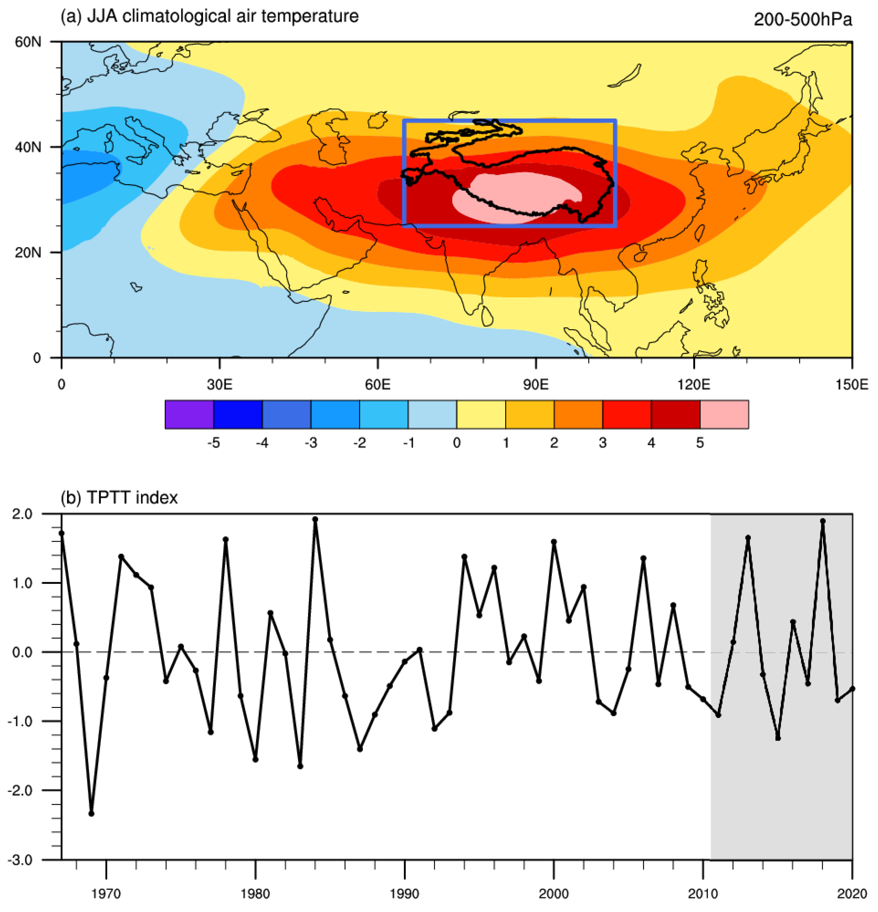
Figure 1a shows a boreal summer climatological tropospheric eddy temperature anomaly at 200–500 hPa over the Asian continent, with the high-temperature center extending from North Africa to the western North Pacific. The peak temperature can reach 5 and is located over the southern TP, with a large warm center found by Li and Yanai [53]. Existing studies indicate that the warming rate of the TP is higher than the average rate in the Northern Hemisphere and almost twice the global mean [54]. Here, the blue box contains the whole TP, which is used to represent the thermal condition over the TP [10,11]. The standardized detrended TPTT sequence is shown in Figure 1b. The value range of the test dataset is from −1.4 to 2.0, which is within the range values of the training dataset (from −2.4 to 2.0). This also partly shows that the training dataset and the test dataset have the same distribution, so it is reasonable for us to divide the training data and test data in this way.
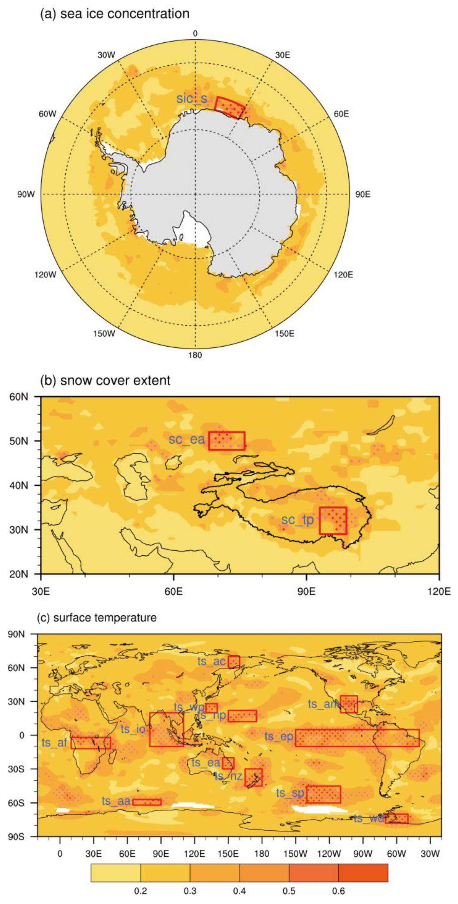
Because XGBoost and LightGBM cannot extract features automatically, we need to select features to train the machine learning models using our expert knowledge. We focus on the seasonal timescale prediction, so we mainly consider the variables with the storage capability of the signals. Considering previous studies on TP heating, the SIC, SC, and TS are selected as the key variables [13,16,17,18,39]. Figure 2 shows the DCORR between the TPTT and the previous boreal spring variables. The significantly correlated regions of the SIC are mainly located around the Antarctic, and the highly correlated regions of SC are over the eastern TP and the Eurasian continent (Figure 2a,b). Compared with the SIC and SC, the TS is closely related to the TPTT at low, middle, and high latitudes (Figure 2c). To ensure the close relationships between these features and the TPTT, we define the regional averaged value in these correlated regions that pass the 99% Monte Carlo test as the features (also known as the predictors). The 15 selected features all show significant connections with the TPTT index (Figure S2). For convenience, the 15 features are abbreviated with variable names and locations in Figure 2. Qian, Jia, Lin, and Zhang [25] also used a similar method for screening features and found it feasible. The 15 features are utilized for training the XGBoost and LightGBM.
Note that significant boreal spring signals corresponding to TPTT exist in two polar areas and middle-to-low latitude areas, especially in the Southern Hemisphere (Figure 2a,c). However, existing studies pay little attention to the Southern Hemisphere precursors of TP heating. In the following, to clarify the importance of each precursor for the predictands, the outputs of the machine learning models are analyzed to evaluate the models’ prediction skills and quantify the importance of the features for the TPTT.
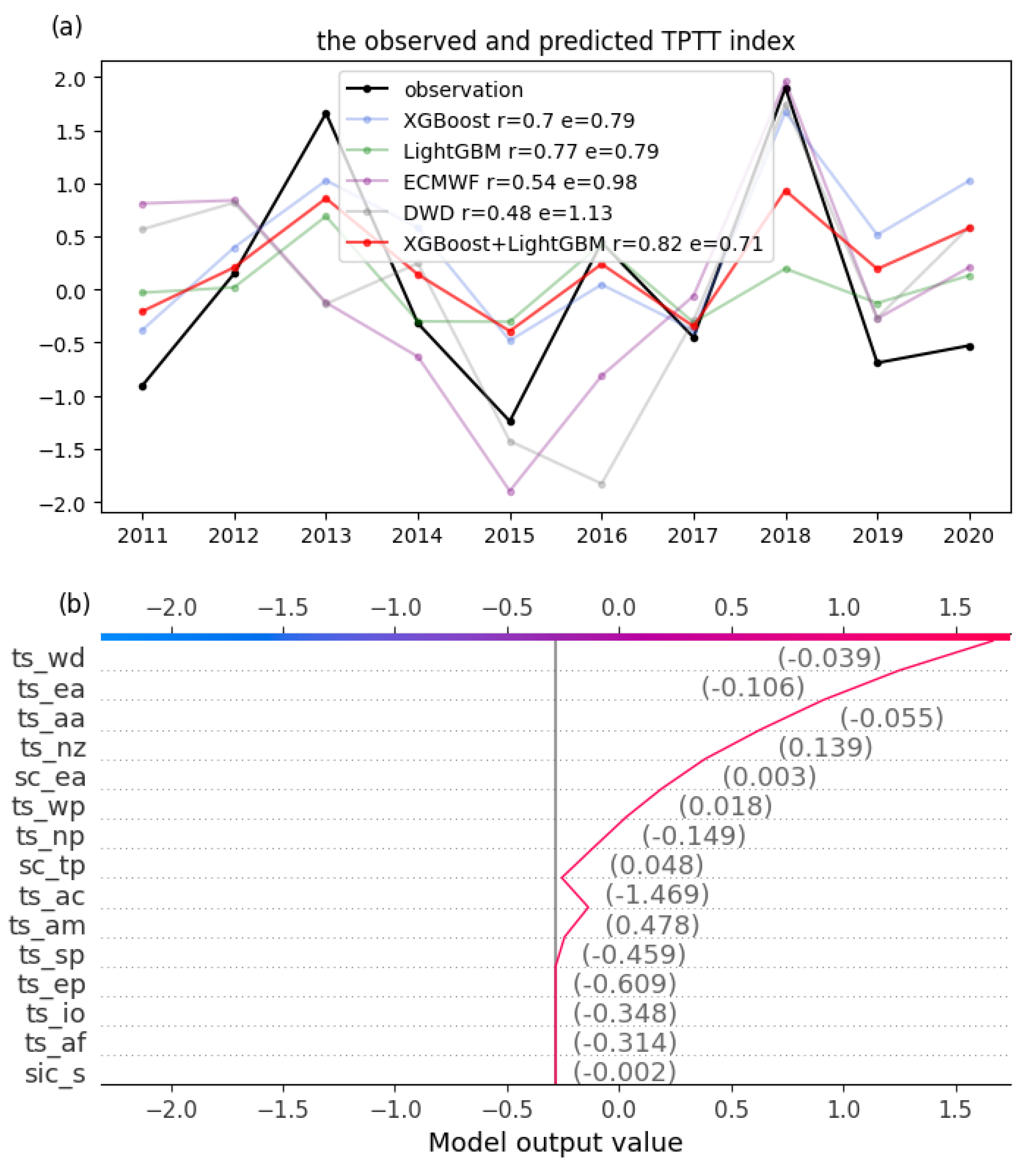
The observed and predicted results of TPTT are shown in Figure 3a. The DCORR between the observation and the prediction of both XGBoost and LightGBM can pass the 95% significance test, and the prediction skills of LightGBM (DCORR = 0.77; RMSE = 0.79) are better than these of the XGBoost (DCORR = 0.7; RMSE = 0.79). The ensemble of both machine learning results can be closer to the observed results (DCORR = 0.82; RMSE = 0.71), which can pass the 99% Monte Carlo test. The hindcasts of the two state-of-the-art models, ECMWF-SEAS5 and DWD-GCFS2.1, are chosen for comparison with the machine learning results, and these two dynamic models show excellent prediction skills on seasonal timescales [55,56]. The DCORRs (RMSEs) between the dynamic model results and the observations are 0.48 (1.13) in DWD-GCFS2.1 and 0.54 (0.98) in ECMWF-SEAS5, which are lower than the machine learning results and cannot pass the 90% significance test. The sign test (sign consistency between the predictions and the observations) of the first-order difference results also indicates that the results of XGBoost and LightGBM are perfectly consistent with the observations. However, only 80% (ECMWF-SEAS5) and 60% (DWD-GCFS2.1) of the predictions are consistent with the observations in these two dynamic models. Therefore, this further illustrates the superiority of the machine learning models over dynamic models for TPTT prediction.
Figure 3a shows that the predictions of the machine learning models are highly consistent with the observations, even in years with an extremely high TPTT index, such as 2018, and the predicted value is very close to the observed value in XGBoost. The extreme year of 2018 is analyzed to understand the prediction model. The decision routine (also known as the decision plot) of the XGBoost model for 2018 is shown in Figure 3b. The trend of the curve represents the accumulation of SHAP values of all features. For example, the value of ts_wd is −0.039 in 2018, and the largest positive SHAP value is in the feature ts_wd, which means that ts_wd contributes greatly to increasing the predicted TPTT value in 2018. In contrast, ts_ac attributes to the decreasing prediction in 2018. There are other features that greatly contribute to the 2018 TPTT value, such as ts_ea, ts_aa, ts_nz, and sc_ea, and these features are mainly from the Southern Hemisphere.
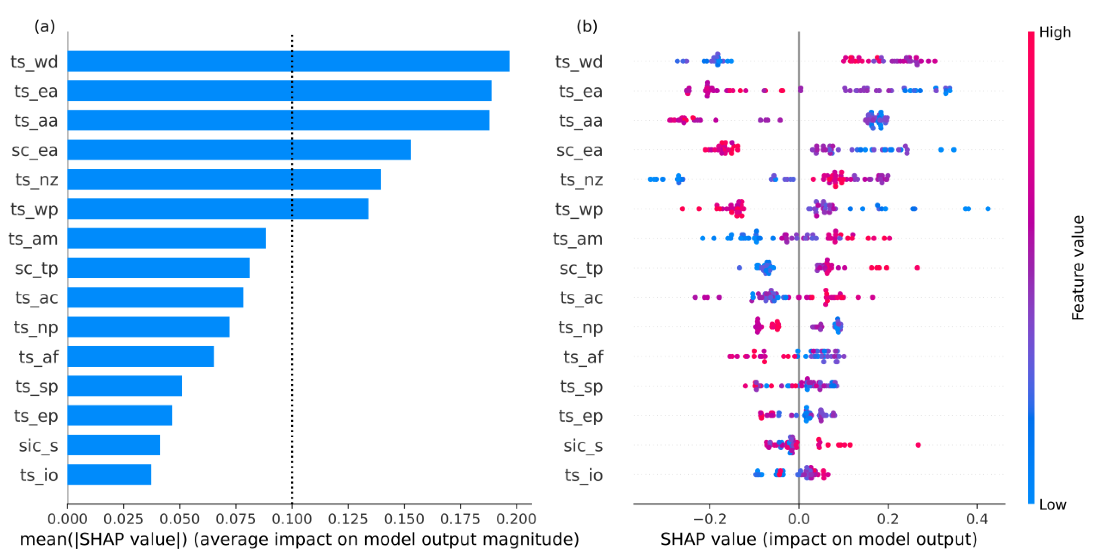
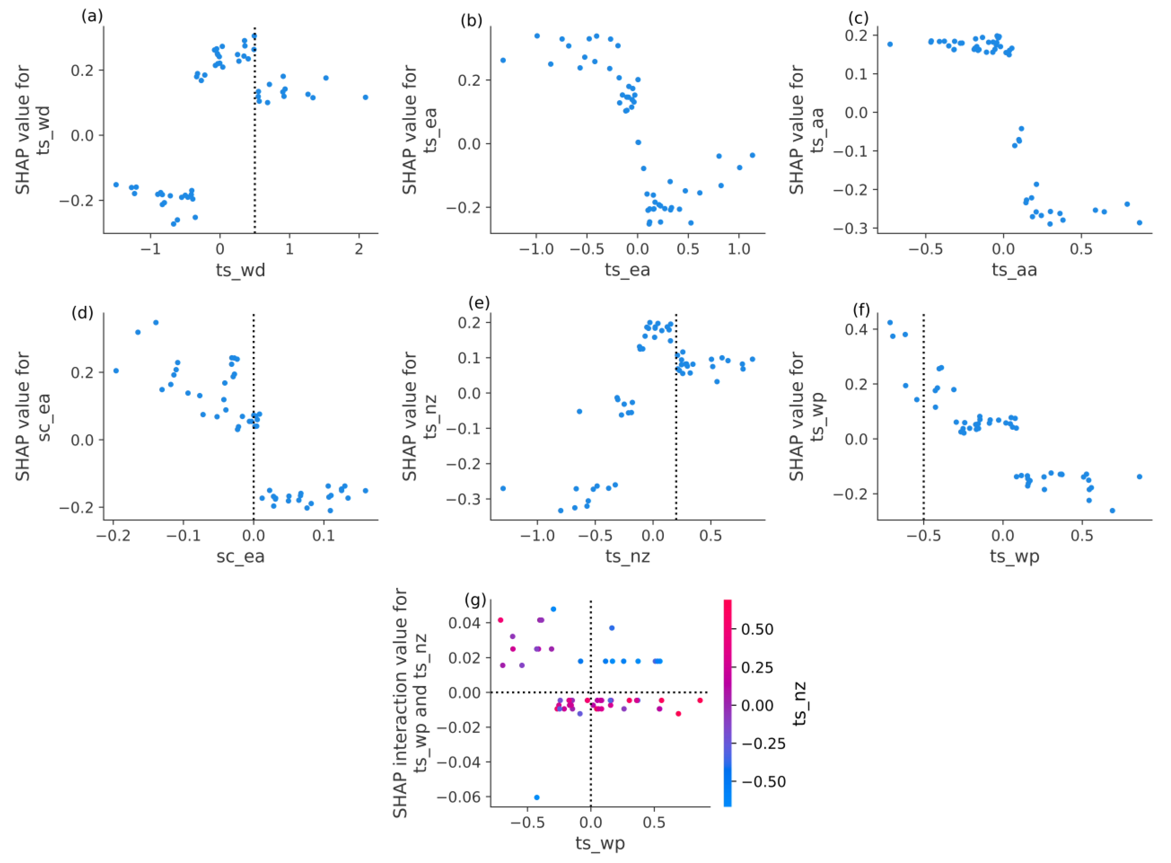
The SHAP analysis of a single sample is not enough to fully understand the logic of the overall prediction of the machine learning models. Therefore, we calculate the global and local feature importance of all the samples. The XGBoost and LightGBM ensemble results of feature importance are shown in Figure 4. The global feature importance in Figure 4a shows the absolute SHAP value average in all the samples, which represents the feature attributions in all the samples, and the ranking importance results are like those of the single sample analysis (Figure 3b). The local feature importance in Figure 4b indicates the distributions of the feature attribution in all the samples. As space is limited in this paper, the most important six features for which the SHAP values are larger than 0.1 are analyzed (Figure 4a). The dependence plots of the six features are shown in Figure 5a–f and are detailed and displayed in Figure 4b. The dependence plot shows the relationship between the feature values and the related SHAP values and can help clarify the influence of the features on the predictands. The large and small feature values of ts_wd are distributed on both sides in Figure 4b. The increase in ts_wd increases the SHAP value of ts_wd, which increases the predicted TPTT index. However, when ts_wd is larger than 0.5, its influence on TPTT weakens, but it still attributes to a larger prediction, showing a nonlinear relationship (Figure 5a). The effect of ts_nz is like that of ts_wd, except that it is a turning point of 0.2 (Figure 5e). The positive feature values of ts_ea and ts_aa correspond to a decrease in the TPTT index and vice versa. In addition, the distribution of these two features exhibits the characteristics of a sign function (Figure 5b,c). As sc_ea increases, the TPTT prediction decreases, but its attribution tends to remain stable after the feature values tend to be positive (Figure 5d). The influence of ts_wp has a long right-tailed distribution, and ts_wp feature values less than −0.5 have great attributions to the increasing TPTT prediction and, there is an obvious linear relationship between the SHAP values of ts_wp and its feature values (Figure 4b and Figure 5f). The above lists the influence of a single feature on the TPTT index. The interaction between two features also affects the TPTT prediction; however, the interaction effects are relatively weak compared to single features (Figure S3). According to the interaction dependence plot, the interaction between ts_nz and ts_wp is chosen. When ts_nz is less than −0.3, and ts_wp is greater than 0, the attribution of this interaction leads to an increase in the TPTT index (Figure 5g).
Most of the important features ranked by the machine learning models and SHAP are in the Southern Hemisphere. The TS anomaly in the eastern Antarctic Peninsula is closely related to the Antarctic Oscillation (AAO), and the in-phase relationship between ts_wd and TPTT further confirms the results of existing studies [19,57]. Ding et al. [58] points out that there is an internal sea surface temperature (SST) quadruple mode in the South Pacific that is driven by the Pacific South American mode, which is similar to the results shown in Figure 2c. Liu et al. [59] and Hsu and Chen [60] indicate that SST anomaly in the South Pacific can influence the western North Pacific and East Asia, which explains the attributions of ts_ea and ts_nz to the subsequent TPTT. Vernekar, Zhou, and Shukla [39] utilize composite analysis to suggest that Eurasian snow cover can decrease the air temperature over the TP, and their results are consistent with our analysis. The Philippine Sea anticyclone teleconnection of the El Niño–South Oscillation leads to a positive SST anomaly in the western North Pacific (ts_wp), which can also induce decreased TPTT [14,61]. In addition, ts_wp may also be linked to the Victoria mode and Pacific Decadal Oscillation and has a vital impact on the SAH and the TPTT [38,62].
4. Discussion
4.1. Uncertainty
SIC data is a product of the fusion of observation data and satellite data, TS data is station-based data, and ERA5 data is a product of the assimilation of observation data, satellite data, and other data. The SC data is pure satellite-based data with uncertainty, so we mainly analyze the uncertainty of SC data. Previous uncertainty assessments of SC suggest that the bias due to illumination, cloud cover, and confounding of SC and other surfaces can lead to overestimation of boreal spring and summer SC in the Arctic and northern Canada [63,64,65]. Although SC data overestimates Arctic SC in June, the SC in boreal spring is consistent with other independent data sets, so our analysis using Eurasian SC data in boreal spring is reliable [66].
4.2. Comparison, Limitations and Contributions
In this paper, the limited observational data are used for seasonal-scale climate prediction and high prediction skills are achieved through two boosting tree models. The random forest model is also utilized. Considering the prediction skill of random forest is poor compared to the boosting tree models, it is not shown in this paper. In meteorology, deep learning and relatively simple machine learning models have been applied to predictions. Due to the powerful fitting ability of deep learning, deep learning models can usually obtain high prediction skills [21,67]. Owing to the large amount of data demanded by deep learning, predictions using numerical simulation data and deep learning need to be further developed, which may further improve prediction skills.
In terms of feature selection, similar feature selection methods (Pearson correlation coefficient screening) and boosting tree models are employed by other researchers for seasonal prediction [25]. Since the Pearson correlation cannot measure the nonlinear relationship, it may miss the features with high nonlinear correlation, so the distance correlation is selected to overcome this problem [52]. The other feature selection methods include the empirical orthogonal function and maximum variance unfolding, etc. [68,69]. These methods are advantageous for the screening of local features. For the selection of global predictors, these methods have obvious limitations. In addition, we also screened the features according to the global climatic annual precipitation, but the correlations between the selected features and the predictand are extremely poor, and the prediction skills were also very low (figures not shown).
In this research, due to the temporal limitation of the data, we use the data from 1967 to 2010 to train the machine learning models, and thus the models only learn the features from the 44 years of data. For signals that do not appear in these 44 years, the prediction skills of the machine learning models are consequentially poor. Therefore, longer time scale datasets should be considered in future studies to improve the generalization ability of the machine learning models. In this paper, we focus on the surface climate variables (SC, SIC, and TS) and do not consider factors of stratospheric signals and other non-meteorological elements, which can also be further studied in the future [70,71].
Previous studies indicate that the Indian Ocean SST has important effects on the SAH and TPTT [13,72,73,74,75]. However, the impact of the Indian Ocean (ts_io) is underestimated in the machine learning models, and similar results also appear in the deep learning method related to the EASM [26]. This underestimation problem is still unresolved in machine learning, so we need to be careful to avoid the underestimation of the Indian Ocean in future studies. Nonlinear relationships in the climate system are often ignored in quantitative studies. However, the vital impacts of these nonlinear interactions should be given sufficient attention (Figure 5). By comparing our results with previous studies, we find that some features, such as ts_aa, show a very important predictive significance in machine learning models, but there is no corresponding research on this subject. Therefore, further research is needed to verify whether such a physical connection exists.
In this paper, the data used are heterogeneous, such as SC, SIC, and TS, with different physical meanings. SHAP is used to transform heterogeneous features with different physical meanings into uniform ones under the nature of additivity. The observed datasets from 1967 to 2010 are used to train the statistical machine learning models; however, the results still need to be examined in terms of climate dynamics theories and numerical simulations. Therefore, the analysis results obtained by SHAP are a quasi-explanation, not the final explanation, but it is nevertheless meaningful for revealing objective phenomena (connections) that are not yet discovered, which helps to fill the gap in the interpretability of machine learning models of the TPTT. In addition, there are few studies on the prediction of TP heat source and its interpretability, our prediction based on machine learning and the SHAP method may provide ideas for the operational prediction and precursor studies.
5. Conclusions
This paper employs two machine learning models (XGBoost and LightGBM) and the SHAP method to predict the TPTT index and analyze its key precursors. Expert knowledge and distance correlation are applied to extract highly correlated features, which are supported by theoretical knowledge. Both linear and nonlinear relationships are considered in choosing the features. The features are fed into the machine learning models to obtain a final prediction. The prediction skills of the two machine learning models can pass the 99% significance test (DCORR = 0.82), with an RMSE of 0.71. The prediction skills of both state-of-the-art dynamic models (ECMWF-SEAS5 and DWD-GCFS2.1) are lower than the prediction skills of the machine learning models, which indicates that machine learning models can significantly improve the prediction of TPTT. By using the SHAP method, we find that the importance of the features in all the samples is ranked from high to low as follows: ts_wd, ts_ea, ts_aa, sc_ea, ts_nz, ts_wp, ts_am, sc_tp, ts_ac, ts_np, ts_af, ts_sp, ts_ep, sic_s, and ts_io. The six most important features that attribute the most to the TPTT prediction are mainly located in the Southern Hemisphere, the western North Pacific, and Eurasia, and most of these features have nonlinear relationships with the TPTT. The influences of these most important features on the TPTT are generally consistent with the existing studies.
Supplementary Materials
The following supporting information can be downloaded at: https://0-www-mdpi-com.brum.beds.ac.uk/article/10.3390/rs14174169/s1, Figure S1: The TPTT, the meridional location index of the SAH and two East Asian summer monsoon (EASM) index; Figure S2: The DCORRs between the 15 features and the TPTT index from 1967 to 2010; Figure S3: The interaction summary plot of the most important six features [76,77,78].
Author Contributions
Conceptualization, Y.T. and A.D.; Methodology, Y.T.; Software, Y.T. and C.X.; Validation, Y.T., A.D. and Y.X.; Formal Analysis, Y.T. and A.D.; Writing—Original Draft Preparation, Y.T.; Writing—Review and Editing, Y.T., A.D., C.X. and Y.X.; Visualization, Y.T.; Supervision, A.D. All authors have read and agreed to the published version of the manuscript.
Funding
The work was supported by Strategic Priority Research Program of the Chinese Academy of Sciences (Grant No. XDA19070404) and National Natural Science Foundation of China (Grant No. 42030602).
Data Availability Statement
The data presented in this study are available on request from the corresponding author.
Acknowledgments
The sea ice concentration dataset is from the Met Office Hadley Centre (https://www.metoffice.gov.uk/hadobs/hadisst2/data/download.html; accessed date: 30 December 2021). The NOAA Climate Data Record of Northern Hemisphere Snow Cover Extent is from https://www.ncei.noaa.gov/access/metadata/landing-page/bin/iso?id=gov.noaa.ncdc:C00756 (accessed date: 30 December 2021). The Berkeley Earth temperature is from http://berkeleyearth.org/data/ (accessed date: 6 December 2021). The air temperature datasets are from ERA5 (https://cds.climate.copernicus.eu/cdsapp#!/dataset/reanalysis-era5-pressure-levels-monthly-means-preliminary-back-extension?tab=form and https://cds.climate.copernicus.eu/cdsapp#!/dataset/reanalysis-era5-pressure-levels-monthly-means?tab=form; accessed date: 19 November 2021). The hindcast data of the two dynamic models (ECMWF-SEAS5 and DWD-GCFS2.1) are from https://cds.climate.copernicus.eu/cdsapp#!/dataset/seasonal-monthly-pressure-levels?tab=form (accessed date: 6 January 2022).
Conflicts of Interest
The authors declare no conflict of interest.
References
- Ye, D.; Gao, Y. Meteorology of the Qinghai-Xizang (Tibet) Plateau; Science Press: Beijing, China, 1979; p. 316. (In Chinese) [Google Scholar]
- Wu, G.; Duan, A.; Liu, Y.; Mao, J.; Ren, R.; Bao, Q.; He, B.; Liu, B.; Hu, W. Tibetan Plateau climate dynamics: Recent research progress and outlook. Natl. Sci. Rev. 2014, 2, 100–116. [Google Scholar] [CrossRef]
- Wu, G.; Liu, Y.; He, B.; Bao, Q.; Duan, A.; Jin, F.-F. Thermal Controls on the Asian Summer Monsoon. Sci. Rep. 2012, 2, 404. [Google Scholar] [CrossRef]
- Liu, Y.; Lu, M.; Yang, H.; Duan, A.; He, B.; Yang, S.; Wu, G. Land–atmosphere–ocean coupling associated with the Tibetan Plateau and its climate impacts. Natl. Sci. Rev. 2020, 7, 534–552. [Google Scholar] [CrossRef]
- Lai, X.; Gong, Y. Relationship between atmospheric heat source over the Tibetan Plateau and precipitation in the Sichuan–Chongqing region during summer. J. Meteorol. Res. 2017, 31, 555–566. [Google Scholar] [CrossRef]
- Zhao, P.; Chen, L. Interannual variability of atmospheric heat source/sink over the Qinghai—Xizang (Tibetan) Plateau and its relation to circulation. Adv. Atmos. Sci. 2001, 18, 106–116. [Google Scholar] [CrossRef]
- Ye, D.; Luo, S.; Zhu, B. The wind structure and heat balance in the lower troposphere over Tibetan Plateau and its surrounding. Acta Meteorol. Sin. 1957, 28, 108–121. (In Chinese) [Google Scholar]
- Wu, G.; Zhang, Y. Tibetan Plateau Forcing and the Timing of the Monsoon Onset over South Asia and the South China Sea. Mon. Weather Rev. 1998, 126, 913–927. [Google Scholar] [CrossRef]
- Wu, G.; He, B.; Liu, Y.; Bao, Q.; Ren, R. Location and variation of the summertime upper-troposphere temperature maximum over South Asia. Clim. Dyn. 2015, 45, 2757–2774. [Google Scholar] [CrossRef]
- Nan, S.; Zhao, P.; Chen, J. Variability of summertime Tibetan tropospheric temperature and associated precipitation anomalies over the central-eastern Sahel. Clim. Dyn. 2019, 52, 1819–1835. [Google Scholar] [CrossRef]
- Nan, S.; Zhao, P.; Chen, J.; Liu, G. Links between the thermal condition of the Tibetan Plateau in summer and atmospheric circulation and climate anomalies over the Eurasian continent. Atmos. Res. 2021, 247, 105212. [Google Scholar] [CrossRef]
- Zhu, Y.-Y.; Yang, S. Evaluation of CMIP6 for historical temperature and precipitation over the Tibetan Plateau and its comparison with CMIP5. Adv. Clim. Chang. Res. 2020, 11, 239–251. [Google Scholar] [CrossRef]
- Zhao, Y.; Duan, A.; Wu, G. Interannual Variability of Late-spring Circulation and Diabatic Heating over the Tibetan Plateau Associated with Indian Ocean Forcing. Adv. Atmos. Sci. 2018, 35, 927–941. [Google Scholar] [CrossRef]
- Jin, R.; Wu, Z.; Zhang, P. Tibetan Plateau capacitor effect during the summer preceding ENSO: From the Yellow River climate perspective. Clim. Dyn. 2018, 51, 57–71. [Google Scholar] [CrossRef]
- Cui, Y.; Duan, A.; Liu, Y.; Wu, G. Interannual variability of the spring atmospheric heat source over the Tibetan Plateau forced by the North Atlantic SSTA. Clim. Dyn. 2015, 45, 1617–1634. [Google Scholar] [CrossRef]
- Chen, Y.; Duan, A.; Li, D. Connection between winter Arctic sea ice and west Tibetan Plateau snow depth through the NAO. Int. J. Climatol. 2021, 41, 846–861. [Google Scholar] [CrossRef]
- Li, F.; Wan, X.; Wang, H.; Orsolini, Y.J.; Cong, Z.; Gao, Y.; Kang, S. Arctic sea-ice loss intensifies aerosol transport to the Tibetan Plateau. Nat. Clim. Chang. 2020, 10, 1037–1044. [Google Scholar] [CrossRef]
- Shaman, J.; Tziperman, E. The Effect of ENSO on Tibetan Plateau Snow Depth: A Stationary Wave Teleconnection Mechanism and Implications for the South Asian Monsoons. J. Clim. 2005, 18, 2067–2079. [Google Scholar] [CrossRef]
- Liu, Y.; Chen, H.; Li, H.; Wang, H. The Impact of Preceding Spring Antarctic Oscillation on the Variations of Lake Ice Phenology over the Tibetan Plateau. J. Clim. 2020, 33, 639–656. [Google Scholar] [CrossRef]
- Dou, J.; Wu, Z. Southern Hemisphere Origins for Interannual Variations of Snow Cover over the Western Tibetan Plateau in Boreal Summer. J. Clim. 2018, 31, 7701–7718. [Google Scholar] [CrossRef]
- Ham, Y.G.; Kim, J.H.; Luo, J.J. Deep learning for multi-year ENSO forecasts. Nature 2019, 573, 568–572. [Google Scholar] [CrossRef]
- Davenport, F.V.; Diffenbaugh, N.S. Using machine learning to analyze physical causes of climate change: A case study of US Midwest extreme precipitation. Geophys. Res. Lett. 2021, 48, e2021GL093787. [Google Scholar] [CrossRef]
- Jones, N. How machine learning could help to improve climate forecasts. Nature 2017, 548, 379. [Google Scholar] [CrossRef] [PubMed]
- Rasp, S.; Pritchard, M.S.; Gentine, P. Deep learning to represent subgrid processes in climate models. Proc. Natl. Acad. Sci. USA 2018, 115, 9684–9689. [Google Scholar] [CrossRef] [PubMed]
- Qian, Q.; Jia, X.; Lin, H.; Zhang, R. Seasonal Forecast of Non-monsoonal Winter Precipitation over the Eurasian Continent using Machine Learning Models. J. Clim. 2021, 34, 7113–7129. [Google Scholar] [CrossRef]
- Tang, Y.; Duan, A. Using deep learning to predict the East Asian summer monsoon. Environ. Res. Lett. 2021, 16, 124006. [Google Scholar] [CrossRef]
- Xue, M.; Hang, R.; Liu, Q.; Yuan, X.-T.; Lu, X. CNN-based near-real-time precipitation estimation from Fengyun-2 satellite over Xinjiang, China. Atmos. Res. 2020, 250, 105337. [Google Scholar] [CrossRef]
- Li, H.; Yu, C.; Xia, J.; Wang, Y.; Zhu, J.; Zhang, P. A Model Output Machine Learning Method for Grid Temperature Forecasts in the Beijing Area. Adv. Atmos. Sci. 2019, 36, 1156–1170. [Google Scholar] [CrossRef]
- Abdi, A.M. Land cover and land use classification performance of machine learning algorithms in a boreal landscape using Sentinel-2 data. GISci. Remote Sens. 2020, 57, 1–20. [Google Scholar] [CrossRef]
- Wagle, N.; Acharya, T.D.; Kolluru, V.; Huang, H.; Lee, D.H. Multi-Temporal Land Cover Change Mapping Using Google Earth Engine and Ensemble Learning Methods. Appl. Sci. 2020, 10, 8083. [Google Scholar] [CrossRef]
- Talukdar, S.; Singha, P.; Mahato, S.; Shahfahad; Pal, S.; Liou, Y.-A.; Rahman, A. Land-Use Land-Cover Classification by Machine Learning Classifiers for Satellite Observations—A Review. Remote Sens. 2020, 12, 1135. [Google Scholar] [CrossRef]
- Kang, Y.; Ozdogan, M.; Zhu, X.; Ye, Z.; Hain, C.; Anderson, M. Comparative assessment of environmental variables and machine learning algorithms for maize yield prediction in the US Midwest. Environ. Res. Lett. 2020, 15, 064005. [Google Scholar] [CrossRef]
- Zhong, J.; Zhang, X.; Gui, K.; Wang, Y.; Che, H.; Shen, X.; Zhang, L.; Zhang, Y.; Sun, J.; Zhang, W. Robust prediction of hourly PM2.5 from meteorological data using LightGBM. Natl. Sci. Rev. 2021, 8, nwaa307. [Google Scholar] [CrossRef] [PubMed]
- Lee, Y.; Han, D.; Ahn, M.-H.; Im, J.; Lee, S.J. Retrieval of Total Precipitable Water from Himawari-8 AHI Data: A Comparison of Random Forest, Extreme Gradient Boosting, and Deep Neural Network. Remote Sens. 2019, 11, 1741. [Google Scholar] [CrossRef]
- Lundberg, S.M.; Lee, S.-I. A unified approach to interpreting model predictions. In Advances in Neural Information Processing Systems; MIT Press: Cambridge, MA, USA, 2017; Volume 30, pp. 4768–4777. [Google Scholar]
- Lundberg, S.M.; Erion, G.; Chen, H.; DeGrave, A.; Prutkin, J.M.; Nair, B.; Katz, R.; Himmelfarb, J.; Bansal, N.; Lee, S.-I. From local explanations to global understanding with explainable AI for trees. Nat. Mach. Intell. 2020, 2, 56–67. [Google Scholar] [CrossRef]
- Yang, Y.; Yuan, Y.; Han, Z.; Liu, G. Interpretability analysis for thermal sensation machine learning models: An exploration based on the SHAP approach. Indoor Air 2022, 32, e12984. [Google Scholar] [CrossRef] [PubMed]
- Yang, Y.; Su, Q.; Wang, L.; Yang, R.; Cao, J. Response of the South Asian High in May to the early spring North Pacific Victoria Mode. J. Clim. 2022, 35, 3979–3993. [Google Scholar] [CrossRef]
- Vernekar, A.D.; Zhou, J.; Shukla, J. The Effect of Eurasian Snow Cover on the Indian Monsoon. J. Clim. 1995, 8, 248–266. [Google Scholar] [CrossRef]
- Titchner, H.A.; Rayner, N.A. The Met Office Hadley Centre sea ice and sea surface temperature data set, version 2: 1. Sea ice concentrations. J. Geophys. Res.-Atmos. 2014, 119, 2864–2889. [Google Scholar] [CrossRef]
- Robinson, D.A.; Estilow, T.W.; Program, N.C. NOAA Climate Data Record (CDR) of Northern Hemisphere (NH) Snow Cover Extent (SCE) Version 1. 2012. Available online: https://www.ncei.noaa.gov/ (accessed on 30 December 2021). [CrossRef]
- Rohde, R.A.; Hausfather, Z. The Berkeley Earth land/ocean temperature record. Earth Syst. Sci. Data 2020, 12, 3469–3479. [Google Scholar] [CrossRef]
- Chen, T.; Guestrin, C. XGBoost: A Scalable Tree Boosting System. In Proceedings of the 22nd ACM SIGKDD International Conference on Knowledge Discovery and Data Mining, San Francisco, CA, USA, 13–17 August 2022; pp. 785–794. [Google Scholar]
- Ke, G.; Meng, Q.; Finley, T.; Wang, T.; Chen, W.; Ma, W.; Ye, Q.; Liu, T.-Y. Lightgbm: A highly efficient gradient boosting decision tree. In Proceedings of the Advances in Neural Information Processing Systems, Long Beach, CA, USA, 4–9 December 2017; Volume 30, pp. 3147–3155. [Google Scholar]
- Huang, L.; Kang, J.; Wan, M.; Fang, L.; Zhang, C.; Zeng, Z. Solar radiation prediction using different machine learning algorithms and implications for extreme climate events. Front. Earth Sci. 2021, 9, 202. [Google Scholar] [CrossRef]
- Shahhosseini, M.; Hu, G.; Huber, I.; Archontoulis, S.V. Coupling machine learning and crop modeling improves crop yield prediction in the US Corn Belt. Sci. Rep. 2021, 11, 1606. [Google Scholar] [CrossRef] [PubMed]
- Ding, C.; Cao, X.; Næss, P. Applying gradient boosting decision trees to examine non-linear effects of the built environment on driving distance in Oslo. Transp. Res. Part A Policy Pract. 2018, 110, 107–117. [Google Scholar] [CrossRef]
- Akiba, T.; Sano, S.; Yanase, T.; Ohta, T.; Koyama, M. Optuna: A Next-generation Hyperparameter Optimization Framework. In Proceedings of the 25th ACM SIGKDD International Conference on Knowledge Discovery & Data Mining, Anchorage, AK, USA, 4–8 August 2019; pp. 2623–2631. [Google Scholar]
- Chang, I.; Park, H.; Hong, E.; Lee, J.; Kwon, N. Predicting effects of built environment on fatal pedestrian accidents at location-specific level: Application of XGBoost and SHAP. Accid. Anal. Prev. 2022, 166, 106545. [Google Scholar] [CrossRef]
- Barda, N.; Riesel, D.; Akriv, A.; Levy, J.; Finkel, U.; Yona, G.; Greenfeld, D.; Sheiba, S.; Somer, J.; Bachmat, E.; et al. Developing a COVID-19 mortality risk prediction model when individual-level data are not available. Nat. Commun. 2020, 11, 4439. [Google Scholar] [CrossRef] [PubMed]
- Székely, G.J.; Rizzo, M.L.; Bakirov, N.K. Measuring and testing dependence by correlation of distances. Ann. Stat. 2007, 35, 2769–2794. [Google Scholar] [CrossRef]
- Li, R.; Zhong, W.; Zhu, L. Feature Screening via Distance Correlation Learning. J. Am. Stat. Assoc. 2012, 107, 1129–1139. [Google Scholar] [CrossRef]
- Li, C.; Yanai, M. The Onset and Interannual Variability of the Asian Summer Monsoon in Relation to Land–Sea Thermal Contrast. J. Clim. 1996, 9, 358–375. [Google Scholar] [CrossRef]
- You, Q.; Cai, Z.; Pepin, N.; Chen, D.; Ahrens, B.; Jiang, Z.; Wu, F.; Kang, S.; Zhang, R.; Wu, T.; et al. Warming amplification over the Arctic Pole and Third Pole: Trends, mechanisms and consequences. Earth-Sci. Rev. 2021, 217, 103625. [Google Scholar] [CrossRef]
- Johnson, S.J.; Stockdale, T.N.; Ferranti, L.; Balmaseda, M.A.; Molteni, F.; Magnusson, L.; Tietsche, S.; Decremer, D.; Weisheimer, A.; Balsamo, G.; et al. SEAS5: The new ECMWF seasonal forecast system. Geosci. Model Dev. 2019, 12, 1087–1117. [Google Scholar] [CrossRef]
- Fröhlich, K.; Dobrynin, M.; Isensee, K.; Gessner, C.; Paxian, A.; Pohlmann, H.; Haak, H.; Brune, S.; Früh, B.; Baehr, J. The German climate forecast system: GCFS. J. Adv. Model. Earth Syst. 2021, 13, e2020MS002101. [Google Scholar] [CrossRef]
- Wu, Z.; Dou, J.; Lin, H. Potential influence of the November–December Southern Hemisphere annular mode on the East Asian winter precipitation: A new mechanism. Clim. Dyn. 2015, 44, 1215–1226. [Google Scholar] [CrossRef]
- Ding, R.; Li, J.; Tseng, Y.-h. The impact of South Pacific extratropical forcing on ENSO and comparisons with the North Pacific. Clim. Dyn. 2015, 44, 2017–2034. [Google Scholar] [CrossRef]
- Liu, G.; Zhang, Q.; Sun, S. The Relationship between Circulation and SST Anomaly East of Australia and the Summer Rainfall in the Middle and Lower Reaches of the Yangtze River. Chin. J. Atmos. Sci. 2008, 32, 231–241. (In Chinese) [Google Scholar]
- Hsu, H.-H.; Chen, Y.-L. Decadal to bi-decadal rainfall variation in the western Pacific: A footprint of South Pacific decadal variability? Geophys. Res. Lett. 2011, 38, L03703. [Google Scholar] [CrossRef]
- Wang, B.; Wu, R.; Fu, X. Pacific-East Asian Teleconnection: How Does ENSO Affect East Asian Climate? J. Clim. 2000, 13, 1517–1536. [Google Scholar] [CrossRef]
- Xue, X.; Chen, W.; Chen, S.; Feng, J. PDO modulation of the ENSO impact on the summer South Asian high. Clim. Dyn. 2018, 50, 1393–1411. [Google Scholar] [CrossRef]
- Wang, L.; Sharp, M.; Brown, R.; Derksen, C.; Rivard, B. Evaluation of spring snow covered area depletion in the Canadian Arctic from NOAA snow charts. Remote Sens. Environ. 2005, 95, 453–463. [Google Scholar] [CrossRef]
- Brown, R.; Derksen, C.; Wang, L. Assessment of spring snow cover duration variability over northern Canada from satellite datasets. Remote Sens. Environ. 2007, 111, 367–381. [Google Scholar] [CrossRef]
- Déry, S.J.; Brown, R.D. Recent Northern Hemisphere snow cover extent trends and implications for the snow-albedo feedback. Geophys. Res. Lett. 2007, 34, 22. [Google Scholar] [CrossRef]
- Brown, R.; Derksen, C.; Wang, L. A multi-data set analysis of variability and change in Arctic spring snow cover extent, 1967–2008. J. Geophys. Res.-Atmos. 2010, 115, D16. [Google Scholar] [CrossRef]
- Ravuri, S.; Lenc, K.; Willson, M.; Kangin, D.; Lam, R.; Mirowski, P.; Fitzsimons, M.; Athanassiadou, M.; Kashem, S.; Madge, S.; et al. Skilful precipitation nowcasting using deep generative models of radar. Nature 2021, 597, 672–677. [Google Scholar] [CrossRef] [PubMed]
- Lima, C.H.R.; Lall, U.; Jebara, T.; Barnston, A.G. Statistical Prediction of ENSO from Subsurface Sea Temperature Using a Nonlinear Dimensionality Reduction. J. Clim. 2009, 22, 4501–4519. [Google Scholar] [CrossRef]
- Zhao, H.; Lu, Y.; Jiang, X.; Klotzbach, P.J.; Wu, L.; Cao, J. A Statistical Intraseasonal Prediction Model of Extended Boreal Summer Western North Pacific Tropical Cyclone Genesis. J. Clim. 2022, 35, 2459–2478. [Google Scholar] [CrossRef]
- Domeisen, D.I.V.; Butler, A.H.; Charlton-Perez, A.J.; Ayarzagüena, B.; Baldwin, M.P.; Dunn-Sigouin, E.; Furtado, J.C.; Garfinkel, C.I.; Hitchcock, P.; Karpechko, A.Y.; et al. The Role of the Stratosphere in Subseasonal to Seasonal Prediction: 2. Predictability Arising From Stratosphere-Troposphere Coupling. J. Geophys. Res.-Atmos. 2020, 125, e2019JD030923. [Google Scholar] [CrossRef]
- Bibi, S.; Wang, L.; Li, X.; Zhou, J.; Chen, D.; Yao, T. Climatic and associated cryospheric, biospheric, and hydrological changes on the Tibetan Plateau: A review. Int. J. Climatol. 2018, 38, e1–e17. [Google Scholar] [CrossRef]
- Xie, S.-P.; Hu, K.; Hafner, J.; Tokinaga, H.; Du, Y.; Huang, G.; Sampe, T. Indian Ocean Capacitor Effect on Indo–Western Pacific Climate during the Summer following El Niño. J. Clim. 2009, 22, 730–747. [Google Scholar] [CrossRef]
- Xue, X.; Chen, W. Distinguishing interannual variations and possible impacted factors for the northern and southern mode of South Asia High. Clim. Dyn. 2019, 53, 4937–4959. [Google Scholar] [CrossRef]
- Liu, B.; Zhu, C.; Yuan, Y. Two interannual dominant modes of the South Asian High in May and their linkage to the tropical SST anomalies. Clim. Dyn. 2017, 49, 2705–2720. [Google Scholar] [CrossRef]
- Huang, G.; Qu, X.; Hu, K. The impact of the tropical Indian Ocean on South Asian High in boreal summer. Adv. Atmos. Sci. 2011, 28, 421–432. [Google Scholar] [CrossRef]
- Wang, B.; Fan, Z. Choice of South Asian Summer Monsoon Indices. Bull. Amer. Meteorol. Soc. 1999, 80, 629–638. [Google Scholar] [CrossRef]
- Gang, H.; Guijie, Z. The East Asian Summer Monsoon Index (1851–2021); National Tibetan Plateau Data Center: Tibet, China, 2019. [Google Scholar]
- Zhao, G.; Huang, G.; Wu, R.; Tao, W.; Gong, H.; Qu, X.; Hu, K. A New Upper-Level Circulation Index for the East Asian Summer Monsoon Variability. J. Clim. 2015, 28, 9977–9996. [Google Scholar] [CrossRef] [Green Version]
Figure 1.
The eddy tropospheric temperature of 200–500 hPa in boreal summer. The blue box indicates the region of the TPTT index (a). The detrended standardized TPTT sequence. The gray shading indicates the test dataset, and the white background is the training dataset (b).
Figure 1.
The eddy tropospheric temperature of 200–500 hPa in boreal summer. The blue box indicates the region of the TPTT index (a). The detrended standardized TPTT sequence. The gray shading indicates the test dataset, and the white background is the training dataset (b).

Figure 2.
The distance correlation between TPTT and boreal spring SIC (a), SC (b), and TS (c) from 1967 to 2010. The pink and red dots indicate the 95% and 99% Monte Carlo tests. The red boxes are the selected feature regions, and the blue text to the left of the red box is the abbreviation of each feature. The sic_s means the feature is selected from SIC in South Hemisphere. And the definition of other features are similar as follows: SC in Eurasia (sc_ea), SC in the Tibetan Plateau (sc_tp), TS in Arctic (ts_ac), TS in western Pacific (ts_wp), TS in northern Pacific (ts_np), TS in America (ts_am), TS in Africa (ts_af), TS in Indian Ocean (ts_io), TS in eastern Pacific (ts_ep), TS in eastern Australia (ts_ea), TS in New Zealand (ts_nz), TS in Antarctica (ts_aa), TS in South Pacific (ts_sp), TS in Weddell Sea (ts_wd).

Figure 3.
The observed and predicted TPTT index by using the boreal spring initial fields. The r and e values represent the DCORR and RMSE between the prediction and the observation, respectively (a); The decision routine of the TPTT index in 2018 by using XGBoost. The vertical coordinate of (b) is the feature importance ranking, with decreasing importance from top to bottom, and the values next to the curve are the corresponding feature values. The upper end of the curve is the final prediction for 2018 (b).

Figure 4.
The global (a) and local (b) feature importance in all samples. Each dot in (b) represents one sample, and the colors of the dots represent the values of the sample features (also known as feature values).
Figure 4.
The global (a) and local (b) feature importance in all samples. Each dot in (b) represents one sample, and the colors of the dots represent the values of the sample features (also known as feature values).

Figure 5.
The dependence plots of six important features (a–f). The interaction dependence plot of ts_wp and ts_nz (g). The dots indicate the samples.
Figure 5.
The dependence plots of six important features (a–f). The interaction dependence plot of ts_wp and ts_nz (g). The dots indicate the samples.

Publisher’s Note: MDPI stays neutral with regard to jurisdictional claims in published maps and institutional affiliations. |
© 2022 by the authors. Licensee MDPI, Basel, Switzerland. This article is an open access article distributed under the terms and conditions of the Creative Commons Attribution (CC BY) license (https://creativecommons.org/licenses/by/4.0/).
Share and Cite
MDPI and ACS Style
Tang, Y.; Duan, A.; Xiao, C.; Xin, Y. The Prediction of the Tibetan Plateau Thermal Condition with Machine Learning and Shapley Additive Explanation. Remote Sens. 2022, 14, 4169. https://0-doi-org.brum.beds.ac.uk/10.3390/rs14174169
AMA Style
Tang Y, Duan A, Xiao C, Xin Y. The Prediction of the Tibetan Plateau Thermal Condition with Machine Learning and Shapley Additive Explanation. Remote Sensing. 2022; 14(17):4169. https://0-doi-org.brum.beds.ac.uk/10.3390/rs14174169
Chicago/Turabian StyleTang, Yuheng, Anmin Duan, Chunyan Xiao, and Yue Xin. 2022. "The Prediction of the Tibetan Plateau Thermal Condition with Machine Learning and Shapley Additive Explanation" Remote Sensing 14, no. 17: 4169. https://0-doi-org.brum.beds.ac.uk/10.3390/rs14174169
Note that from the first issue of 2016, this journal uses article numbers instead of page numbers. See further details here.