
Correlation Analysis of CO2 Concentration Based on DMSP-OLS and NPP-VIIRS Integrated Data


1
School of Electronic Information, Wuhan University, Wuhan 473072, China
2
Hubei Luojia Laboratory, Wuhan 430079, China
3
Tianjin Nautical Instrument Research Institute, Tianjin 300131, China
4
State Key Laboratory of Information Engineering in Surveying, Mapping and Remote Sensing, Wuhan University, Wuhan 473079, China
*
Author to whom correspondence should be addressed.
Remote Sens. 2022, 14(17), 4181; https://0-doi-org.brum.beds.ac.uk/10.3390/rs14174181
Submission received: 8 August 2022
/
Revised: 20 August 2022
/
Accepted: 22 August 2022
/
Published: 25 August 2022
(This article belongs to the Special Issue Optical and Laser Remote Sensing of Atmospheric Composition)
Abstract
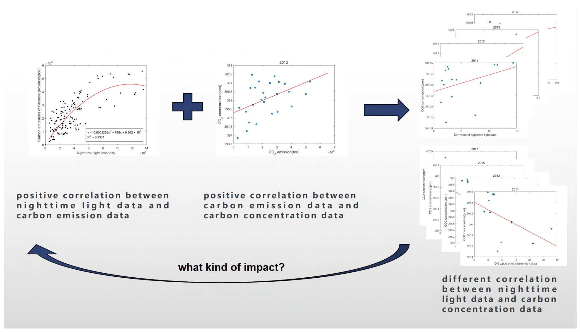
:In view of global warming, caused by the increase in the concentration of greenhouse gases, China has proposed a series of carbon emission reduction policies. It is necessary to obtain the spatiotemporal distribution of carbon emissions accurately. Nighttime light data is recognized as an important basis for carbon emission estimation. A large number of research results show that there is a positive correlation between nighttime light intensity and carbon emission. However, in the current context of China’s industrial reforms, this positive relationship may not be entirely correct. First, we correct the nighttime light data from different satellites and established a long-term series data set. Then, we verify the positive correlation between nighttime light and carbon emission. However, the time scale of emission data often lags, and the carbon concentration data are released earlier and are more accurate than emission data. Therefore, we propose to investigate the relationship between nighttime light and carbon concentration. It is found that there may be different correlations between nighttime light and the carbon concentration, due to different urban industrial structure and development planning. Therefore, by exploring the relationship between nighttime light and the carbon concentration, the existing carbon emission estimation model can be modified to improve the accuracy of the emission model.

1. Introduction
Energy is an important material basis for human existence and production. With the continuous progress of human society, people’s demand for energy is increasing day by day. China’s current energy structure is still largely dependent on fossil fuels, such as oil, coal, and natural gas [1]. The burning of fossil fuels has led to a gradual increase in greenhouse gas emissions. According to the World Bank, China’s CO2 emissions in 1990 were only 2.46 billion tons, which accounts for 11% of the global total, and are far lower than the United States’ 4.879 billion tons. Since 2005, China’s total CO2 emission (including LUCF) has ranked first in the world. Additionally, China’s total CO2 emissions were about 10 billion tons in 2018, accounting for about 28% of the global total, which is about twice that of the United States and 9.2 times that of Russia. The massive emission of CO2 not only affects the sustainable development strategy but also causes great harm to the environment, the most obvious feature of which is global warming [2]. Therefore, energy saving and emission reduction to reduce CO2 emissions are some of the important tasks at present. In response to the call for a low-carbon economy and green development, China announced during the APEC meeting at the end of 2014 that it planned to peak CO2 emissions around 2030 and strove to do so as early as possible. In addition, China planned to increase the share of non-fossil energy in primary energy consumption to about 20% by 2030. China reaffirmed its goal of “Emission Peak” by 2030 and “Carbon Neutrality” by 2060 in September 2020. In order to effectively implement the dual carbon target, the task of carbon emission reduction needs to be carefully assigned to local administrative units. Thus, we need to be able to accurately analyze the spatiotemporal changes of carbon emissions [3].
There are two main methods of estimating carbon emissions. One approach is the statistics-based IPCC carbon accounting method, which is a common way of estimating carbon emissions. Schipper et al. [4] used the IPCC inventory method to analyze the evolution of carbon emissions from the manufacturing sector in 13 IEA countries. Nejat et al. [5] estimated the carbon emissions of ten countries, including China, the United States, and India, based on energy consumption, and they proved that the residential sector is the third largest energy consumer in the world. However, most of these carbon emissions estimates are based on national, regional, and provincial scales. Due to incomplete data, it is difficult to estimate carbon emissions on the county or even grid scale. The other is an observation-based approach (top-down estimate of carbon emissions) to estimating carbon emissions, one of which is to estimate carbon emissions from nighttime light data. The Satellite Nighttime Light (NL) sensors are capable of recording visible light, which can reflect the dynamics of human activities to some extent [6]. Carbon emissions (Carbon, in this paper, mainly comes from CO2.) are also deeply affected by human activities, so many scholars use NL data to estimate carbon emissions. Ma et al. [7] used the corrected DMSP-OLS data to construct a spatiotemporal geographically weighted regression model between NL data and carbon emissions per capita, as well as carbon emissions per unit area in China. The evaluation results showed that there was a good correlation between NL data and carbon emission data, which could better simulate the spatiotemporal dynamics of carbon emissions. Wang et al. [8] analyzed the carbon emission estimation model of Guangdong Province, based on NTL, and revealed the scale effect law of different spatial resolutions. Moreover, in order to synthesize the advantages of both kinds of NL data and study the relationship between long-term NL data and carbon emission data, many scholars have integrated these data. Li et al. mainly integrated nighttime light data by synthesizing monthly NPP-VIIRS data, from 2012 to 2018, into annual data [9]. Qian et al. [10] constructed a NL data set and used it to establish an estimation model for CO2 emissions. On this basis, they analyzed the spatiotemporal dynamics of CO2 emissions at four scales: pixel, county, prefecture, and province.
Numerous studies have shown that there is a positive correlation between NL data and carbon emission data, and NL data are used to estimate CO2 emissions in the establishment of a carbon emission estimation model. However, considering that China is currently implementing carbon emission reduction policies to control regional carbon emissions, especially in some developed cities such as Beijing and Shanghai, the marginalization of heavy industry appears. In developed cities with high NL intensity, CO2 emissions can be low. Therefore, the positive correlation between NL data and carbon emission data, in the carbon emission estimation model, may not be completely correct, so this paper studies whether there is a negative correlation. Since the time scale of emission data often lags, carbon concentration data are released relatively earlier, and the data accuracy is higher. Therefore, we choose to study the relationship between NL data and carbon concentration data.
In this study, we firstly process DMSP-OLS and NPP-VIIRS data to obtain long-term NL data, and then, we use the integrated NL data to verify the positive correlation between NL data and carbon emission data in China. At the same time, previous studies show that carbon emissions, caused by industrial emissions and human activities, will affect atmospheric CO2 concentration, and the carbon concentration should also be high in areas with high carbon emissions [11,12]. Therefore, it can be theoretically inferred that there should also be a positive correlation between NL data and CO2 concentration. This view can be verified by comparing the night-light remote sensing images and the spatial distribution maps of CO2 concentration in Hubei Province. However, when studying the relationship between NL data and CO2 concentration in prefecture-level cities in the Beijing–Tianjin–Hebei region, it is found that there is a negative correlation. Therefore, this paper aims at the reason why there is a negative correlation between NL data and CO2 concentration in the Beijing–Tianjin–Hebei region, and it provides a new idea for the further improvement of the model of estimating carbon emissions based on NL data.
2. Data Sources
Multiple data sets are used in this study, including DMSP-OLS NL images [13], NPP-VIIRS NL images [14], MODIS EVI product [15], CO2 emission data [16], and CO2 concentration data [17] in China.
DMSP is the Defense Weather Satellite Program of the United States. The program detects low-intensity lights at night through sensors carried by weather satellites. The National Oceanic and Atmospheric Administration (NOAA) collects statistics and, then, publishes annual data of global stable nighttime lights. From 1992 to 2013, there were 34 periods of stable NL data from DMSP-OLS, which were obtained from six satellites (F10, F12, F14, F15, F16, and F18). Each period of data has three types: stable NL data, cloud-free coverage, and average visible image. These three types of data are available as GeoTIFFs for download from the version 4 composites in NOAA/NGDC. The nighttime light data values are saturated, ranging from 1 to 63, and the background noise is identified and replaced with zero values.
NPP-VIIRS satellite data also come from the National Geophysical Center of the U.S. National Oceanic and Atmospheric Administration. The first Suomi National Polar Cooperation satellite was launched in the United States in October 2011. At present, the Suomi-NPP satellite only provides daily data, monthly synthetic data, and some annual synthetic data from 2012 to the present. The NPP-VIIRS nighttime light data are not oversaturated and have a resolution of 15 arc seconds (about 500 m at the equator).
The MODIS EVI product is a 16-day composite image data available from Google Earth Engine. The MOD13A2 product used in this study provides two vegetation indices (VI): normalized differential vegetation index (NDVI) and enhanced vegetation index (EVI). EVI data can be used to desaturate DMSP data. The algorithm of the product is to select the best available pixel value from the images collected within 16 days, with a resolution of 1 km.
CO2 emission data are obtained from the Multi-resolution Emission Inventory for China (MEIC). Since 2010, MEIC has been developed and maintained by Tsinghua University to build a high-resolution inventory of anthropogenic air pollutants and CO2 emissions in China. It covers more than 700 anthropogenic emission sources in mainland China, including 10 major air pollutants and carbon dioxide (SO2, NOX, CO, NMVOC, NH3, PM2.5, PM10, BC, OC, and CO2) emissions.
The CO2 concentration data are obtained from the Monthly Global Map of the CO2 column-averaged volume mixing ratios provided by GOSAT, which are processed to obtain CO2 concentration data with high spatiotemporal resolution [18].
Based on the data sets described above and other data sets used in this paper but not introduced in detail, the information sources of all data sets used in this paper are shown in Table 1.
3. NL Data Preprocessing
Due to the limitations of OLS sensor design, there are problems such as discontinuities between DMSP-OLS night-light remote sensing images and oversaturation of pixel DN value. Additionally, DMSP data are provided until 2013 and, then, replaced by NPP-VIIRS NL data. NPP-VIIRS data have been available since April 2012, but NL images have problems with background noise and outliers. Therefore, in order to obtain long-term stable NL data values, two types of data need to be corrected and carried on data fitting. The process of data fitting is shown in Figure 1.
Firstly, two types of NL data are processed, respectively. Due to its different characteristics, DMSP-OLS data require inter-sensor correction, continuity correction, and desaturation. NPP-VIIRS data require annual data synthesis and noise reduction. Then, the linear model is used to regress the two kinds of data after processing, and the relationship between them is obtained. The DMSP-OLS data are integrated into NPP-VIIRS data to obtain the NL data of long-term series.
3.1. Correcting DMSP-OLS Data
DMSP-OLS stabilized nighttime light radiation data are obtained from different sensors. After removing the unstable light sources, such as auroras and wildfires, as well as the interference of moonlight and clouds, the final data are the stable average annual value of the cloudless images [20]. The 34 periods of NL data, from 1992 to 2013, are obtained by six satellites respectively. Due to the decline of satellites and the different performance of different sensors in detection, the image data of different sensors are discontinuous in different years. For example, compared with other sensors, F18 has a mutation. There is a big leap between the data obtained in 2009 by F16 and that obtained in 2010 by F18. In addition, the data obtained by different sensors in the same year also differ. For instance, the total DN value obtained by F15 and F16 in 2004 differ by 28.4%. Therefore, inter-sensor calibration of DMSP-OLS data is required. The calibration process is as follows.
Firstly, Jixi City of Heilongjiang Province, with stable urban development and a wide range of regional night light DN value, is selected as a pseudo invariant region. F16 is selected as the standard sensor, and the stable NL data obtained by F16 from 2004 to 2009 are used as the reference data set. Then, the F15 data are corrected with the F16 NL data. The F16 and F15 data overlap from 2004 to 2007, so the image metadata of Jixi from F162004 to F162007 are used as reference. The least square method is used to fit the data from F152004 to F152007 with a quadratic regression model. The F15 sensor data are corrected with the obtained parameters, and then, the F14 sensor data are corrected with the corrected F15 sensor data. In this way, the corrected F14, F12, and F10 can be obtained. Since there is no data of coincident year between the F16 sensor and F18 sensor, the data of F162009 are used to perform quadratic regression on the data of F182010, and the corrected F18 data are obtained. The regression equation is shown in Equations (1) and (2).
In the expression, indicates the DN value of the reference data set. indicates the DN value of the data to be corrected set. indicates the DN value of the raw data before correction. indicates the DN value of the corrected data set. n indicates the sensor number, and n − 1 indicates the previous sensor number. a, b, and c indicate parameters determined by fitting progress. Parameters of the sensor calibration regression model are shown in Table 2.
Due to the absence of on-board calibration, there are abnormal fluctuations among the data obtained by the same sensor in different years. In addition, there are differences in the data obtained by different sensors. Therefore, DMSP NL data are discontinuous in long-term series, so continuity correction is needed. Firstly, the differences generated by different sensors on the data of the same year are processed, according to Equation (3), to obtain the only stable NL data set for each year from 1992 to 2013.
In the expression, n indicates the year. and represent the DN values of two sensors in n year.
According to the law of urban development in China, the DN value of NL data in the next year should not be lower than that of the previous year. Therefore, the Equation (4) is adopted for correction:
In the expression, and represent the DN values of the sensor in n and n − 1 year.
Moreover, the DN value, influenced by DMSP night-light remote sensing images, has a saturation effect, while NPP-VIIRS data have no saturation effect. Therefore, to integrate DMSP-OLS data into NPP-VIIRS data, Enhanced Vegetation Index (EVI) can be used to desaturate DMSP data. The MODIS EVI product is 16-day composite image data provided by NASA LP DAAC at the USGS EROS Center. There are 23 issues of data per year, with an average of two issues per month. DMSP data are annual average data, so the 23 issues of EVI data are averaged to obtain the annual average EVI image. Then, they are put into the model to desaturate the DMSP data. The formula is shown in Equation (5).
In the expression (5), NTL indicates the DN value of NL data, and nNTL indicates the normalized NTL value. EANTL indicates the NTL value after desaturation.
3.2. Correcting NPP-VIIRS Data
The original satellite observations at NOAA CLASS are easily affected by clouds, moonlight, etc., resulting in cloudy pixels. In addition, the view angle and lunar illumination differences will also affect the data and need radiometric adjustments [21]. The NPP-VIIRS data used in this study are based on monthly cloud-free composites produced by the Earth Observation Group (EOG). The monthly average light radiation data product, synthesized by VIIRS/DNB, has been published monthly since April 2014. The images are filtered for stray light, lightning, moonlight, and clouds, and they retain auroras, fire, boats, and other temporary lights. Therefore, abnormal values may occur in the data, which need the reduction in noise. This experiment refers to Zhong’s [22] method and uses the VIIRS annual composite night light data of 2015, which has been filtered by American authorities, as a mask for noise reduction. First, the annual VIIRS data of 2015 are binarized, the value of the light area is assigned as 1, and the value of the non-light area is assigned as 0. Then, the image is used as a mask, and raster multiplication is performed with the data of the image to be processed on the grid’s scale. The result is that the original value of the light area in 2015 is retained, and the light value of the non-light area is changed to 0.
3.3. Processing Result
We compare the preprocessing data with the post-processing data. Figure 2 shows DMSP data from 2008 to 2013 and synthetic VIIRS annual data from 2013 to 2017 before processing. Figure 3 shows the NL data from 2008 to 2017 after processing. From the figures, it can be found that the NL data have a large span before processing, and there is a mutation phenomenon. The data, after processing, are more consistent with the actual law.
3.4. Regression Analysis
Many scholars choose to convert VIIRS data into DMSP data. However, considering that CO2 concentration has monthly data, it is more convenient and effective to use VIIRS monthly data for discussion. Moreover, the spatial resolution of the original DMSP and VIIRS data are 2.7 km and 742 m, respectively, so the VIIRS data can provide more spatial detail. Moreover, VIIRS DNB has a wider radiation range and stronger low-light detection ability compared to DMSP. Therefore, this paper chooses to convert DMSP data into VIIRS data to obtain long-term series NL data. DMSP-OLS provides annual data from 1992–2013, and NPP-VIIRS provides monthly data from April 2012 to the present, so NL data from overlapping years are used for fitting. DMSP-OLS provides annual data, and NPP-VIIRS data from January to March 2012 are missing, so 2013 data are used for fitting. The monthly data of VIIRS in 2013 are synthesized into annual data by means of the average method, and then, the sum of provincial regional pixels of DMSP-OLS and NPP-VIIRS nighttime lights in 2013 are counted, respectively, and fitted by linear regression model. The result is shown in Figure 4.
In Figure 4, the dots represent Chinese provinces. Tibet, Hong Kong, Macao, and Taiwan were excluded from the study due to the lack of complete information. The abscissa is DMSP data and the ordinate is VIIRS data. It can be seen from the figure that DMSP, in 2013, has a good linear correlation with VIIRS data, and the fitting degree can reach 0.8733 by using the linear model, indicating that this regression model is highly representative. Therefore, a regression equation was obtained to integrate DMSP-OLS data with NPP-VIIRS data. The formula is shown in Equation (6).
In the expression, x indicates the total value of provincial area DN of raw DMSP-OLS NL data, and y indicates the DN value corrected to NPP-VIIRS data. According to the above formula, the longstanding NL data from 1992 have been obtained.
4. Analysis of Experiment
In recent years, many scholars have studied the correlation between NL data and carbon emission data, and they have constructed carbon emission estimation models based on NL data. In order to realize spatial informatization of carbon emissions, Zhao et al. [23] constructed a simulation model of carbon emissions in the Yangtze River Delta region, from the pixel scale, by using NL data and energy consumption statistics as data sources. Xiao et al. [24] used DMSP-OLS and NPP-VIIRS to construct a NL data set with a long-term series. Combined with energy statistics, they established a relationship model between NL values and urban energy carbon emissions in Hunan Province, and they further simulated the urban energy carbon emissions in its time series. It can be found that there is a positive correlation between NL data and carbon emission data. To further verify it, this paper studies the relationship between NL data and carbon emission data on a provincial scale.
Since China’s existing statistical data cannot directly provide the carbon emission data of regions or industries, the carbon emission data can only be obtained, indirectly, through statistical data. At present, there are many carbon emission products, such as ODIAC [25,26,27,28]. Considering that the experiment is conducted in China and has the same spatial resolution as the carbon concentration data, this experiment uses the annual, sector-wide (including power, industry, transport, civil, and agricultural) CO2 emission data from the MEIC Inventory from 2008 to 2017, with a resolution of 0.25°. Since the NL data of the long-term series are obtained by fitting the data of 2013, the NL data of 2013 and carbon emission data are selected for the study. In order to make the research results more reliable, the data from 2008 to 2017 are taken to make regression with the carbon emission data. The fitting result is shown in Figure 5.
In Figure 5, the dots represent Chinese provinces. Tibet, Hong Kong, Macao, and Taiwan were excluded from the study due to the lack of complete information. The abscissa is NL intensity and the ordinate is carbon emissions. Due to excessive data, only odd-year data are used in Figure 5. NL data adopt the total intensity of regional light, i.e., the sum of DN values of all pixels in a province in China. Carbon emission data are also the total carbon emissions of each province. It can be seen from Figure 5 that there is a positive correlation between NL data and carbon emission data. Places with large DN values of NL light have frequent social and economic activities, leading to an increase in carbon emissions. This is also consistent with the existing carbon emission estimation model, that is, NL data as the input are considered to have a positive correlation with carbon emissions [29].
Moreover, Figure 6 is a statistical chart of the total DN value of annual nighttime light and the total carbon emission of Beijing from 2008 to 2017. Comparing the long-term series NL data with the carbon emission data, we can find that the results basically satisfy that, when the nighttime light intensity is high, the carbon emissions rise. Besides, when the intensity is low, the carbon emissions are also reduced, which verifies the positive correlation between NL data and carbon emissions and further validates the conclusions of current research.
Research has shown that carbon emission caused by human activities is the main reason for the increase in global CO2 concentration. In order to control the continuous rise of CO2 concentration, all countries in the world are committed to anthropogenic carbon emission reduction measures [30]. The change of CO2 concentration data is taken as one of the foundations of judging the effect of emission reduction policy implementation [31]. At present, many scholars have studied the relationship between CO2 concentration and carbon emissions. He et al. [32] found that the area with high spatial difference of near-surface CO2 concentration was significantly correlated with human carbon emissions and was significantly affected by human activities. Diao et al. [33] found, through experiments, that CO2 concentration was high in areas with more factories and less vegetation, and vice versa, indicating that anthropogenic carbon emissions had an important impact on CO2 concentration. In addition, Deng et al. [34] revealed the substitution relationship between CO2 emissions and CO2 concentration, under the same temperature, rises by proving the substitution elasticity of CO2 emissions and CO2 concentration on warming. Thus, there is a positive correlation between carbon emissions and the carbon concentration.
Then, we use the total carbon emissions and average CO2 concentration data of each province in China, in 2013, to conduct a fitting to testify to the conclusion. As shown in Figure 7, the dots represent Chinese provinces. Tibet, Hong Kong, Macao, Taiwan, the Nei Monggol Autonomous Region and Heilongjiang Province were excluded from the study due to the lack of complete information. The abscissa is the total carbon emission of China’s provincial administrative divisions, and the ordinate is the average CO2 concentration of China’s provincial administrative divisions. It can be seen from Figure 7 that most of these spots with high carbon emissions also have high average CO2 concentration. The above conclusion can be further verified. Therefore, we theoretically speculate that there should also be a positive correlation between NL data and CO2 data. Then, results are verified by studying the night-light remote sensing images and the spatial distribution map of CO2 concentration in each region.
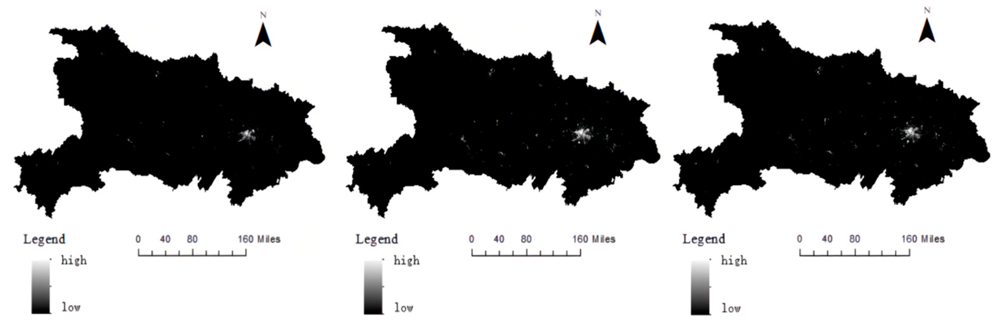
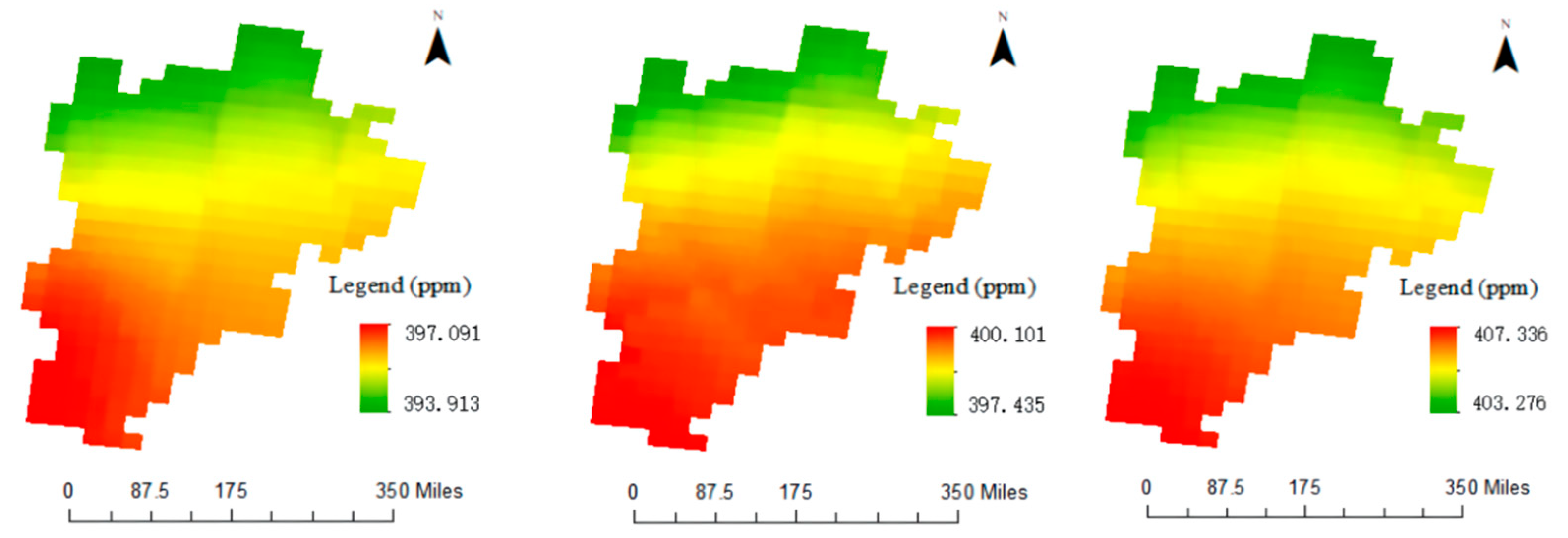
Firstly, we study night-light remote sensing images and the spatial distribution of CO2 concentration in Hubei Province from 2013 to 2017. The nighttime light images are the monthly average NL data after noise reduction processing. The resolution of the NPP-VIIRS image is 500 m, and the resolution of the CO2 concentration image is 25 km. NL images have higher resolution and, therefore, provide more detailed information. The detection of CO2 column concentration by satellite is easily disturbed by cloud cover, aerosols, and other factors, resulting in the limited spatial resolution of CO2 concentration. Meanwhile, CO2 has an atmospheric diffusion effect, which makes it impossible to obtain the information of strong emission point sources. The spatial resolution of our CO2 concentration data is low, so the local area with strong CO2 concentration caused by similar power plants cannot be clearly shown on the concentration map. Therefore, we choose to discuss on the prefecture scale. It can be seen from Figure 8 and Figure 9 that the intensity of night-light gradually increased over these five years, and so did the concentration of CO2. In addition, it is obvious that CO2 concentration is also higher in places with higher NL intensity, which is basically consistent with the above conclusion that there is a positive correlation between NL data and CO2 concentration data. To further verify it, we conduct a linear fitting of NL data and CO2 concentration data in cities in Hubei province. The relatively complete data of CO2 concentration are available from 2010, while the carbon emission data start from 2008 to 2017. Therefore, considering the data integrity and coincidence, we choose to study the relationship between the average annual NL data and carbon concentration from 2010 to 2017. The average intensity of nighttime light of cities in Hubei Province is extracted from the annual NL data after fusion, which is the average value of NL data DN in each region. CO2 concentration has a diffusion effect, so it make no sense to use the total value of CO2 concentration to study. The average CO2 concentration in each region is used in the test. The fitting results are shown in Figure A1 in Appendix A. In these figures, the abscissas are the average DN value of NL data in the region, and the ordinates are the average CO2 concentration in the region. It is found that there is a positive correlation between NL data and carbon concentration data.
Since monthly data of CO2 concentration are available, in order to better discuss the relationship between NL and CO2 concentration, we select the monthly data of NPP-VIIRS from 2013 to 2017 for the study. The mean NL intensity of prefecture-level cities in Hubei province is extracted from NPP-VIIRS data after pretreatment, that is, the mean NL data DN of each region. Due to the large amount of data, the data are represented by the results of two months each year. The fitting results are shown in Figure A2 in Appendix A. It can be seen from the results that there is also a positive correlation between monthly NL data and CO2 concentration data.
When studying the correlation between the average NL data and the carbon concentration data of Hubei Province, from 2010 to 2017, we can find that the average nighttime light intensity of Wuhan is much higher than that of other cities when VIIRS data are used. However, when using DMSP data to extract NL data of cities in Hubei provinces, this situation does not occur. This is because the VIIRS DNB band has high radiation sensitivity, and some radiance information from gas combustion and fire may also lead to outliers in the data. Therefore, the maximum value is removed before studying the relationship between NL data and carbon concentration data in Hubei Province
However, in the study of night-light remote sensing images and CO2 concentration distribution maps in the Beijing–Tianjin–Hebei region, it can obviously be found that the conclusion is not consistent with the above inference. As shown in Figure 10 and Figure 11, in the Beijing–Tianjin–Hebei region, the NL intensity of Beijing and Tianjin is obviously greater than that of other regions, but the CO2 concentration distribution diagram shows that the CO2 concentration in the Beijing–Tianjin–Hebei region is the largest part mainly in Hebei Province. Therefore, we further explore the relationship between NL intensity and CO2 concentration through the linear fitting of NL data and CO2 concentration data, from 2010 to 2017, in the Beijing–Tianjin–Hebei region.
Figure A3 in Appendix A shows the fitting results between the annual NL data and the CO2 concentration data in cities of the Beijing–Tianjin–Hebei region from 2010 to 2017. Selected areas are Beijing, Tianjin, and Hebei prefecture-level administrative regions (Chengde, Qinhuangdao, and Zhangjiakou are not included in the study because of their low NL intensity, due to their relatively backward economy). It is found that there is a negative correlation between NL data and carbon concentration data. Moreover, we also used the monthly data of NPP-VIIRS, from 2013 to 2017, for the study. March and August are selected as representatives. It is obvious that there is also a negative correlation between two sets of data, as shown in the Figure A4 in Appendix A. Beijing and Tianjin are relatively developed, with frequent social and economic activities, and the total intensity of lights at night is relatively high [35]. Therefore, Beijing and Tianjin are the two points on the far right of the figures, respectively. It can be seen that the CO2 concentration is lower than that of the surrounding Hebei region. This result is inconsistent with the previous inference. Therefore, through consulting materials and literature, it is found that, although the Beijing–Tianjin–Hebei region is closely connected, its development gradient is greatly different, and the contradiction between economic development and environmental resources is obvious [36]. Current regional economic development is in different stages [37]. The core industries of heavy industry, such as raw material supply and the energy supply, are mainly concentrated in Hebei City, while the core industries of light industry and the service industry are mainly concentrated in the Tianjin and Beijing regions [38]. As a result, some prefecture-level cities in Hebei province have higher carbon emissions than Beijing and Tianjin. In addition, as the capital of China and an international metropolis, Beijing has made remarkable achievements in environmental governance, low carbon emissions reduction, and other aspects. By actively adjusting and optimizing industrial structure and promoting green industrial development, the decoupling between economic development and carbon emissions has been preliminarily achieved [39]. Therefore, the urban economy of Beijing and Tianjin is developing rapidly, but the CO2 emissions in Hebei province play a dominant role in the whole region. As a result, there is a negative correlation between the nighttime light intensity and the CO2 concentration data in the Beijing–Tianjin–Hebei region.
The existing models for estimating carbon emissions from NL data almost assume that carbon emissions increase with the increase in NL intensity. However, with the adjustment of China’s industrial and energy structure, carbon emissions will reach the “Emission peak” in the future and even gradually decrease. Therefore, when using the carbon emission model to estimate the future carbon emissions, the implementation effect of the current carbon emission reduction policy should be considered, and the carbon emissions should be estimated in combination with the actual situation. In addition, it can be seen from the above research results that heavy industry may be marginalized in some developed regions, leading to carbon emissions mainly concentrated in some underdeveloped regions. Therefore, when simulating the spatial distribution of carbon emissions in various regions, the local industrial structure and emission policies should also be taken into account to make the results more practical. In the current study, Ou et al. [40] used multiple sources of data, including NL data, population density data, and road grid data, to jointly estimate carbon emissions. Su et al. [41] estimated the carbon emissions of prefecture-level cities in China with the assistance of a Landsat remote sensing image by using the relationship between NL data and carbon emission statistics. Zhao et al. [42] estimated the energy consumption of prefecture-level cities in China by combining the nighttime light data and the gross regional product, and the results were accurate and feasible to a certain extent. On this basis, they analyzed the impact of changes in China’s industrial structure on China’s energy consumption. Ghosh et al. [43] proposed the combination of nighttime light data and population data to build a carbon emission estimation model. The results show that these methods are more accurate than the carbon emission data generated by NL data alone. Therefore, the subsequent research intends to establish a new carbon emission estimation model, based on the surface vegetation structure, industrial structure, and other data, to further verify and study the experimental results.
5. Conclusions
In this paper, the pre-processed DMSP-OLS data and NPP-VIIRS data are fitted to obtain the nighttime light data of long-term series. Then, we regress the NL data of more than 30 provinces in China with total carbon emissions, and we find a positive correlation between NL data and carbon emission. Since there is a positive correlation between carbon emission data and carbon concentration data, NL data should also be positively correlated with carbon concentration data. The conclusion is verified by comparing night-light remote sensing images with the spatial distribution maps of CO2 concentration. In Hubei province, it is obvious that the CO2 concentration is high in places with high NL intensity, which is consistent with the above inferred results. However, when studying the Beijing–Tianjin–Hebei region, it is found that CO2 concentration is lower in places with high NL intensity in Beijing and Tianjin. Therefore, in order to further study, the NL data and CO2 concentration data in the Beijing–Tianjin–Hebei region are fitted, and a long-term negative correlation is found between them. After analysis, it should be caused by the industrial structure and carbon emission policies of the Beijing–Tianjin–Hebei region. The heavy industry in Beijing and Tianjin is gradually marginalized, while light industry and service industries develop rapidly, so the NL intensity is high, but the CO2 concentration is low. Some areas of Hebei province have a high CO2 concentration due to the concentration of heavy industry with high carbon emissions. Therefore, when constructing the model to estimate carbon emissions using NL data, factors such as industrial structure, carbon emission policy, and the urbanization level of the study area should be taken into account to optimize the model and make the estimate result closer to the actual situation. In addition, a carbon emission estimation model with NL data removed can be established at the same time, and then, the research results of the two models can be compared to find out the specific significance of NL data in the carbon emission estimation model. Since CO2 diffusion’s influence is not considered in this study, this influence can be studied to explore whether it will affect the regression between NL data and carbon concentration data. Additionally, the subsequent research can use longer time series data to study.
Author Contributions
Conceptualization, C.Z. and X.M.; Data curation, Z.G.; Formal analysis, X.M.; Investigation, C.Z.; Methodology, X.M.; Resources, W.G. and R.W.; Software, C.Z.; Supervision, X.M.; Validation, W.G., Z.G. and D.K.; Visualization, D.K. and R.W.; Writing—original draft, C.Z. and X.M.; Writing—review & editing, C.Z. and X.M. All authors will be informed about each step of manuscript processing including submission, revision, revision reminder, etc. via emails from our system or assigned Assistant Editor. All authors have read and agreed to the published version of the manuscript.
Funding
This work was supported by the National Natural Science Foundation of China (Grant No.42171464,41971283,41801261,41827801,41801282), The Key Research and Development Project of Hubei Province (2021BCA216), and LIESMARS Special Research Funding.
Acknowledgments
DMSP-OLS data presented in this study are openly available in NOAA at https://www.ngdc.noaa.gov/eog/dmsp/downloadV4composites.html, (accessed on 25 April 2022) [13]. NPP-VIIRS data presented in this study are openly available in NOAA at https://www.ngdc.noaa.gov/eog/viirs/download_ut_mos.html, (accessed on 25 April 2022) [14]. EVI data presented in this study are openly available in Google Earth Engine at https://lpdaac.usgs.gov/products/mod13a2v061, (accessed on 12 June 2022) [15]. CO2 concentration data presented in this study are openly available in Gosat Project at https://data2.gosat.nies.go.jp/gallery/fts_l2_swir_co2_gallery_en.html, (accessed on 5 May 2022) [17]. CO2 emission data presented in this study are openly available in Multi-resolution Emission Inventory for China at http://meicmodel.org, (accessed on 5 May 2022) [16]. The administrative boundaries of China presented in this study are openly available in National Geographic Center of China at http://www.ngcc.cn/ngcc, (accessed on 24 April 2022) [19].
Conflicts of Interest
The authors state that they have no conflict of interest.
Appendix A. Fitting Figures
Figure A1.
Correlation between annual NL data and CO2 concentration of cities in Hubei province from 2010 to 2017.
Figure A1.
Correlation between annual NL data and CO2 concentration of cities in Hubei province from 2010 to 2017.

Figure A2.
Correlation between monthly NL data and CO2 concentration of cities in Hubei province from 2013 to 2017.
Figure A2.
Correlation between monthly NL data and CO2 concentration of cities in Hubei province from 2013 to 2017.

Figure A3.
Correlation between annual NL data and CO2 concentration of cities in Beijing-Tianjin-Hebei region from 2010 to 2017.
Figure A3.
Correlation between annual NL data and CO2 concentration of cities in Beijing-Tianjin-Hebei region from 2010 to 2017.

Figure A4.
Correlation between monthly NL data and CO2 concentration of cities in Beijing-Tianjin-Hebei region from 2013 to 2017.
Figure A4.
Correlation between monthly NL data and CO2 concentration of cities in Beijing-Tianjin-Hebei region from 2013 to 2017.

References
- He, Y.; Lin, B. Forecasting China’s total energy demand and its structure using ADL-MIDAS model. Energy 2018, 151, 420–429. [Google Scholar] [CrossRef]
- Liu, B.; Ma, X.; Ma, Y.; Li, H.; Jin, S.; Fan, R.; Gong, W. The relationship between atmospheric boundary layer and temperature inversion layer and their aerosol capture capabilities. Atmos. Res. 2022, 271, 106121. [Google Scholar] [CrossRef]
- Dong, Y.; Shi, W.; Du, B.; Hu, X.; Zhang, L. Asymmetric Weighted Logistic Metric Learning for Hyperspectral Target Detection. IEEE Trans. Cybern. 2021, 1–14. [Google Scholar] [CrossRef] [PubMed]
- Schipper, L.; Murtishaw, S.; Khrushch, M.; Ting, M.; Karbuz, S.; Unander, F. Carbon emissions from manufacturing energy use in 13 IEA countries: Long-term trends through 1995. Energy Policy 2001, 29, 667–688. [Google Scholar] [CrossRef]
- Nejat, P.; Jomehzadeh, F.; Taheri, M.M.; Gohari, M.; Majid, M.Z.A. A global review of energy consumption, CO 2 emissions and policy in the residential sector (with an overview of the top ten CO 2 emitting countries). Renew. Sustain. Energy Rev. 2015, 43, 843–862. [Google Scholar] [CrossRef]
- Yu, B.; Tang, M.; Wu, Q.; Yang, C.; Deng, S.; Shi, K.; Peng, C.; Wu, J.; Chen, Z. Urban Built-Up Area Extraction From Log- Transformed NPP-VIIRS Nighttime Light Composite Data. IEEE Geosci. Remote Sens. Lett. 2018, 15, 1279–1283. [Google Scholar] [CrossRef]
- Ma, Z.; Xiao, H. Spatiotemporal simulation study of China’s provincial carbon emissions based on satellite night lighting data. China Popul. Resour. Environ. 2017, 27, 143–150. [Google Scholar]
- Wang, Y.; Wang, M.; Li, S.; Lin, Y. Scale effect analysis of carbon emission simulation based on NPP-VIIRS images in Guangdong Province. Bull. Surv. Mapp. 2021, 11, 25–30. [Google Scholar] [CrossRef]
- Li, X.; Zhou, Y.; Zhao, M.; Zhao, X. A harmonized global nighttime light dataset 1992–2018. Sci. Data 2020, 7, 168. [Google Scholar] [CrossRef]
- Lv, Q.; Liu, H.; Wang, J.; Liu, H.; Shang, Y. Multiscale analysis on spatiotemporal dynamics of energy consumption CO2 emissions in China: Utilizing the integrated of DMSP-OLS and NPP-VIIRS nighttime light datasets. Sci. Total Environ. 2020, 703, 134394. [Google Scholar] [CrossRef]
- Liu, L.X.; Zhou, L.X.; Xia, L.J.; Wang, H.Y.; Fang, S.X. Establishment and assessment of QA/QC method for sampling and analysis of atmosphere background CO2. Environ. Sci. 2014, 12, 4482–4488. [Google Scholar] [CrossRef]
- Yang, C.Y.; Wang, H.J.; Han, S.J.; Zhao, S.X. Climate simulation for dynamic heterogeneous distribution of atmospheric CO2 concentration. Chin. J. Geophys. 2012, 55, 2809–2825. [Google Scholar]
- NOAA National Centers for Environmental Information (NCEI). DMSP-OLS[EB/OL]. Available online: https://www.ngdc.noaa.gov/eog/dmsp/downloadV4composites.html (accessed on 25 April 2022).
- NOAA National Centers for Environmental Information (NCEI). NPP-VIIRS[EB/OL]. Available online: https://www.ngdc.noaa.gov/eog/viirs/download_ut_mos.html (accessed on 25 April 2022).
- Didan, K. MODIS/Terra Vegetation Indices 16-Day L3 Global 1km SIN Grid V061 [Data Set]. NASA EOSDIS Land Processes DAAC. 2021. Available online: https://lpdaac.usgs.gov/products/mod13a2v061 (accessed on 12 June 2022).
- Li, M.; Liu, H.; Geng, G.; Hong, C.; Liu, F.; Song, Y.; Tong, D.; Zheng, B.; Cui, H.; Man, H.; et al. Anthropogenic emission inventories in China: A review. Natl. Sci. Rev. 2017, 4, 834–866. [Google Scholar] [CrossRef]
- Zhang, H.; Ma, X. Monthly-Averaged XCO2 in Global. Figshare. Dataset. 2022. Available online: https://figshare.com/articles/dataset/WHUXCO2-GLOBAL/17826404/2 (accessed on 5 May 2022).
- Ma, X.; Zhang, H.; Han, G.; Mao, F.; Xu, H.; Shi, T.; Hu, H.; Sun, T.; Gong, W. A Regional Spatiotemporal Downscaling Method for CO2 Columns. IEEE Trans. Geosci. Remote Sens. 2021, 59, 8084–8093. [Google Scholar] [CrossRef]
- National Geomatics Center of China. Administrative boundaries of China [EB/OL]. Available online: http://www.ngcc.cn/ngcc/ (accessed on 24 April 2022).
- Cao, H.; Li, X.; Tong, Z. Impact of Image Saturation on Radiometric Intercalibration of DMSP/OLS Nighttime Light Images. IEEE J. Sel. Top. Appl. Earth Obs. Remote Sens. 2021, 14, 7948–7960. [Google Scholar] [CrossRef]
- Elvidge, C.D.; Hsu, F.C.; Zhizhin, M.; Ghosh, T.; Taneja, J.; Bazilian, M. Indicators of Electric Power Instability from Satellite Observed Nighttime Lights. Remote Sens. 2020, 12, 3194. [Google Scholar] [CrossRef]
- Zhong, L. Monitoring the Economic Development of Countries along the Belt and Road Based on Nighttime Light Remote Sensing Technology. Master’s Thesis, Jiangxi University of Science and Technology, Ganzhou, China, 2020. [Google Scholar] [CrossRef]
- Zhao, J. Spatial-Temporal Variation of Carbon Dioxide Emissions and its Relations to Nighttime Surface Temperature in Yangtze River Delta Region Based on Nightlight Imageries. Master’s Thesis, Yunnan Normal University, Kunming, China, 2020. [Google Scholar] [CrossRef]
- Xiao, Y. Research on Carbon Emission of Urban Energy Consumption in Hunan Province Supported by Nighttime Light Remote Sensing Technology. Master’s Thesis, Jiangxi University of Science and Technology, Ganzhou, China, 2021. [Google Scholar] [CrossRef]
- Oda, T.; Maksyutov, S.; Andres, R.J. The Open-source Data Inventory for Anthropogenic CO2, version 2016 (ODIAC2016): A global monthly fossil fuel CO2 gridded emissions data product for tracer transport simulations and surface flux inversions. Earth Syst. Sci. Data 2018, 10, 87–107. [Google Scholar] [CrossRef]
- Martin, C.R.; Zeng, N.; Karion, A.; Mueller, K.; Ghosh, S.; Lopez-Coto, I.; Gurney, K.; Oda, T.; Prasad, K.; Liu, Y.; et al. Investigating sources of variability and error in simulations of carbon dioxide in an urban region. Atmos. Environ. 2018, 199, 55–69. [Google Scholar] [CrossRef]
- Lin, J.; Lu, S.; He, X.; Wang, F. Analyzing the impact of three-dimensional building structure on CO2 emissions based on random forest regression. Energy 2021, 236, 121502. [Google Scholar] [CrossRef]
- Nassar, R.; Napier-Linton, L.; Gurney, K.R.; Andres, R.J.; Oda, T.; Vogel, F.R.; Deng, F. Improving the temporal and spatial distribution of CO2 emissions from global fossil fuel emission data sets. J. Geophys. Res. Atmos. 2013, 118, 917–933. [Google Scholar] [CrossRef]
- Zhu, E. Study on the Spatial-Temporal Pattern of Carbon Emission and its Response to Urbanization in Zhejiang Province. Ph.D. Dissertation, Zhejiang University, Hangzhou, China, 2020. [Google Scholar] [CrossRef]
- Shi, T.; Han, G.; Ma, X.; Gong, W.; Chen, W.; Liu, J.; Zhang, X.; Pei, Z.; Gou, H.; Bu, L. Quantifying CO2 Uptakes Over Oceans Using LIDAR: A Tentative Experiment in Bohai Bay. Geophys. Res. Lett. 2021, 48, e2020GL091160. [Google Scholar] [CrossRef]
- Lei, L.; Zhong, H.; He, Z.; Cai, B.; Yang, S.; Wu, C.; Zeng, Z.; Liu, L.; Zhang, B. Assessment of atmospheric CO2 concentration enhancement from anthropogenic emissions based on satellite observations. Chin. Sci. Bull. 2017, 62, 2941–2950. [Google Scholar] [CrossRef]
- Jianghao, H.; Yulin, C.; Qin, P. Spatial and temporal variations of carbon dioxide and its influencing factors. Chin. Sci. Bull. 2020, 65, 194–202. [Google Scholar]
- Diao, Y.W.; Huang, J.P.; Liu, C.; Cui, J.; Liu, S.D. A Modeling Study of CO2 Flux and Concentrations over the Yangtze River Delta Using the WRF-GHG Model. Chin. J. Atmos. Sci. 2015, 39, 849–860. [Google Scholar]
- Deng, X.; Jiang, S.-J.; Liu, B.; Wang, Z.-H.; Shao, Q. Statistical analysis of the relationship between carbon emissions and temperature rise with the spatially heterogenous distribution of carbon dioxide concentration. J. Nat. Resour. 2021, 36, 934–947. [Google Scholar] [CrossRef]
- Zhang, J.; Song, M.; Liu, B. Current situation of Carbon dioxide emission and suggestions for emission reduction in China. Nat. Resour. Econ. China 2022, 35, 38–44+50. [Google Scholar] [CrossRef]
- Feng, X.; Li, K. Study on optimization and upgrading of industrial structure of Beijing-Tianjin-Hebei Urban agglomeration. Co-Oper. Econ. Sci. 2022, 8, 20–22. [Google Scholar] [CrossRef]
- Li, J.; Xiang, Y.; Jia, H.; Chen, L. Analysis of Total Factor Energy Efficiency and Its Influencing Factors on Key Energy-Intensive Industries in the Beijing-Tianjin-Hebei Region. Sustainability 2018, 10, 111. [Google Scholar] [CrossRef]
- Zhang, Y. A Study on CO2 Emission Transfer of Different Industries in Beijing-Tianjin-Hebei Region Based on Complex Network. Master’s Thesis, North China Electric Power University, Beijing, China, 2021. [Google Scholar] [CrossRef]
- Han, N.; Luo, X.-Y. Carbon emission peak prediction and reduction potential in Beijing-Tianjin-Hebei region from the perspective of multiple scenarios. J. Nat. Resour. 2022, 37, 1277–1288. [Google Scholar] [CrossRef]
- Ou, J.; Liu, X.; Li, X.; Shi, X. Mapping Global Fossil Fuel Combustion CO2 Emissions at High Resolution by Integrating Nightlight, Population Density, and Traffic Network Data. IEEE J. Sel. Top. Appl. Earth Obs. Remote Sens. 2016, 9, 1674–1684. [Google Scholar] [CrossRef]
- Su, Y.; Chen, X.; Ye, Y.; Wu, Q.; Zhang, H.; Huang, N.; Kuang, Y. The characteristics and mechanisms of carbon emissions from energy consumption in China using DMSP/OLS night light imageries. Acta Geogr. Sin. 2013, 68, 1513–1526. [Google Scholar]
- Zhao, N.; Han, S.; Wang, T. How Does Industrial Restructuring Affect Energy Development in China?—Research on Night Light. China Econ. Stat. Q. 2018, 2, 176–193. [Google Scholar]
- Ghosh, T.; Elvidge, C.D.; Sutton, P.; Baugh, K.E.; Ziskin, D.; Tuttle, B.T. Creating a Global Grid of Distributed Fossil Fuel CO2 Emissions from Nighttime Satellite Imagery. Energies 2010, 3, 1895–1913. [Google Scholar] [CrossRef]
Figure 1.
The process of data fitting.

Figure 2.
Total DN value of nighttime light in Beijing before processing.

Figure 3.
Total DN value of nighttime light in Beijing after processing.

Figure 4.
The fitting result of DMSP-OLS and NPP-VIIR.

Figure 5.
Fitting relationship between NL data and carbon emission data of Chinese provinces.

Figure 6.
Total DN value of nighttime light and total carbon emissions of Beijing.

Figure 7.
Fitting relationship between carbon emissions and the carbon concentration of Chinese provinces.
Figure 7.
Fitting relationship between carbon emissions and the carbon concentration of Chinese provinces.

Figure 8.
Night-light remote sensing images of Hubei province (from left to right, 2013, 2015, 2017).
Figure 8.
Night-light remote sensing images of Hubei province (from left to right, 2013, 2015, 2017).

Figure 9.
Spatial distribution of CO2 concentration in Hubei province (from left to right, 2013, 2015, 2017).
Figure 9.
Spatial distribution of CO2 concentration in Hubei province (from left to right, 2013, 2015, 2017).

Figure 10.
Night-light remote sensing images of Beijing–Tianjin–Hebei region (from left to right: 2013, 2015, 2017).
Figure 10.
Night-light remote sensing images of Beijing–Tianjin–Hebei region (from left to right: 2013, 2015, 2017).

Figure 11.
Spatial distribution of CO2 concentration in Beijing–Tianjin–Hebei region (from left to right: 2013, 2015, 2017).
Figure 11.
Spatial distribution of CO2 concentration in Beijing–Tianjin–Hebei region (from left to right: 2013, 2015, 2017).


Table 1.
Description of the data used in the study.
| Data Set | Description | Time Quantum | Source |
|---|---|---|---|
| DMSP-OLS | 1000 m stable NL data | 1992–2013 | NOAA/NGDC (https://www.ngdc.noaa.gov/eog/dmsp/downloadV4composites.html (accessed on 25 April 2022)) |
| NPP-VIIRS | 500 m NL data | 2013–2021 | NOAA/NGDC (https://www.ngdc.noaa.gov/eog/viirs/download_ut_mos.html (accessed on 25 April 2022)) |
| EVI | Vegetation Index | 2008–2013 | Google Earth Engine (https://lpdaac.usgs.gov/products/mod13a2v061 (accessed on 12 June 2022)) |
| CO2 Emission | 25 km CO2 emission data | 2008–2017 | Multi-resolution Emission Inventory for China (http://meicmodel.org (accessed on 5 May 2022)) |
| CO2 Concentration | 25 km CO2 concentration | 2013–2017 | Gosat Project (https://data2.gosat.nies.go.jp/gallery/fts_l2_swir_co2_gallery_en.html (accessed on 5 May 2022)) |
| Administrative boundaries of China [19] | Vector files of Chinese provinces and cities | National Geographic Center of China (http://www.ngcc.cn/ngcc (accessed on 24 April 2022)) |
Table 2.
Parameters of sensor calibration regression model.
| Sensor Number | a | b | c | R2 |
|---|---|---|---|---|
| F16–F18 | −0.004556 | 1.257 | 1.016 | 0.9172 |
| F16–F15 | 0.001658 | 0.835 | −0.178 | 0.9402 |
| F15–F14 | 0.00005344 | 1.042 | 0.444 | 0.8766 |
| F14–F12 | −0.006385 | 1.371 | −0.699 | 0.9460 |
| F12–F10 | 0.002600 | 0.675 | 0.946 | 0.8743 |
Publisher’s Note: MDPI stays neutral with regard to jurisdictional claims in published maps and institutional affiliations. |
© 2022 by the authors. Licensee MDPI, Basel, Switzerland. This article is an open access article distributed under the terms and conditions of the Creative Commons Attribution (CC BY) license (https://creativecommons.org/licenses/by/4.0/).
Share and Cite
MDPI and ACS Style
Zuo, C.; Gong, W.; Gao, Z.; Kong, D.; Wei, R.; Ma, X. Correlation Analysis of CO2 Concentration Based on DMSP-OLS and NPP-VIIRS Integrated Data. Remote Sens. 2022, 14, 4181. https://0-doi-org.brum.beds.ac.uk/10.3390/rs14174181
AMA Style
Zuo C, Gong W, Gao Z, Kong D, Wei R, Ma X. Correlation Analysis of CO2 Concentration Based on DMSP-OLS and NPP-VIIRS Integrated Data. Remote Sensing. 2022; 14(17):4181. https://0-doi-org.brum.beds.ac.uk/10.3390/rs14174181
Chicago/Turabian StyleZuo, Chen, Wei Gong, Zhiyu Gao, Deyi Kong, Ruyi Wei, and Xin Ma. 2022. "Correlation Analysis of CO2 Concentration Based on DMSP-OLS and NPP-VIIRS Integrated Data" Remote Sensing 14, no. 17: 4181. https://0-doi-org.brum.beds.ac.uk/10.3390/rs14174181
Note that from the first issue of 2016, this journal uses article numbers instead of page numbers. See further details here.