Estimating LAI for Cotton Using Multisource UAV Data and a Modified Universal Model

Abstract

Leaf area index(LAI) is an important indicator of crop growth and water status. With the continuous development of precision agriculture, estimating LAI using an unmanned aerial vehicle (UAV) remote sensing has received extensive attention due to its low cost, high throughput and accuracy. In this study, multispectral and light detection and ranging (LiDAR) sensors carried by a UAV were used to obtain multisource data of a cotton field. The method to accurately relate ground measured data with UAV data was built using empirical statistical regression models and machine learning algorithm models (RFR, SVR and ANN). In addition to the traditional spectral parameters, it is also feasible to estimate LAI using UAVs with LiDAR to obtain structural parameters. Machine learning models, especially the RFR model (R² = 0.950, RMSE = 0.332), can estimate cotton LAI more accurately than empirical statistical regression models. Different plots and years of cotton datasets were used to test the model robustness and generality; although the accuracy of the machine learning model decreased overall, the estimation accuracy based on structural and multisources was still acceptable. However, selecting appropriate input parameters for different canopy opening and closing statuses can alleviate the degradation of accuracy, where input parameters select multisource parameters before canopy closure while structural parameters are selected after canopy closure. Finally, we propose a gap fraction model based on a LAI_max threshold at various periods of cotton growth that can estimate cotton LAI with high accuracy, particularly when the calculation grid is 20 cm (R² = 0.952, NRMSE = 12.6%). This method does not require much data modeling and has strong universality. It can be widely used in cotton LAI prediction in a variety of environments.

1. Introduction

Leaf area index (LAI) is defined as half of the total leaf area per unit ground surface area. [1], which is an important indicator of crop growth and water consumption [2]. Conventional methods of LAI measurement include destructive sampling of plant samples and indirect optical acquisition, both with disadvantages such as a small spatial range, time-consumptive and laborious, with measurement errors easily influenced by human factors [3,4]. Using remote sensing imagery allows a new method to estimate LAI with large-scale and nondestructive characteristics [5,6,7]. However, satellite remote sensing data are highly susceptible to adverse weather conditions and have low spatial and temporal resolution [8]. UAVs carrying high-resolution sensors can effectively solve these problems, and they have been widely used in monitoring crop growth indicators in recent years [9,10,11,12].

UAV remote sensing technology is divided into two categories: optical passive remote sensing and LiDAR active remote sensing [13]. That is, the vegetation indices are calculated by passively acquiring the canopy reflectance through UAVs equipped with multi-spectral or hyperspectral cameras, and the vegetation structure information is acquired by UAVs equipped with LiDAR actively emitting a laser with the ability to penetrate the canopy. Constructing statistical regression models to estimate LAI using the correlation between VIs, structural parameters and LAI is the most common means, such as estimating LAI through NDVI [14], and in forestry, tree structural parameters (height, strength and density) are measured using LiDAR to build allometric models for research and analysis [15,16]. The method is simple and practical but not very accurate. With the advent of artificial intelligence, some machine learning algorithms such as Random Forest Regression (RFR), Support Vector Regression (SVR), Ridge Regression (RR) and Artificial Neural Network (ANN) have performed well in crop phenotype monitoring [17,18,19]. Machine learning can process large datasets and solve nonlinear problems with high accuracy and robustness. However, LiDAR is usually applied to taller plants, and in optical remote sensing in dense cropping patterns or the late stage of crop growth, the light saturation effect due to canopy closure makes the estimation results low [20,21]. Therefore, the applicability of UAV equipped with LiDAR for estimating LAI of low crops and the model’s accuracy under different canopy structures are yet to be evaluated. Research has also shown that the model estimation accuracy can be improved by fusing data from multiple sensors [21,22,23]. Therefore, it is significant to find the most suitable model framework to fuse multi-sensor data for low-growth crops.

The gap fraction model based on Beer–Lambert’s law to estimate LAI is a universal physical model widely used in forestry, as it does not require large amounts of measured data for modeling but has high prediction accuracy. It is obtained using reflectance ratios: ground point clouds to the total number of cloud points [24], ground return point intensity to total intensity [25] and the ground return energy to the total return energy [26]. Additional methods calculate the gap fraction, analyze the correlation between the LAI and the gap fraction and then estimate the vegetation LAI.

The estimation of LAI by the gap fraction model can be affected by many factors, including grid size, leaf distribution, height threshold, noise and ground point classification [13]. Among these, the calculation grid size will directly affect the estimation accuracy. If the calculation grid is too large, it cannot fulfill the monitoring requirements, while too small of a calculation grid will lead to the maximum values in some grids. Some studies opt to select a larger grid, remove the maximum value or define 10 as the calculation threshold to solve the equation [27,28,29,30]. However, the changing pattern of LAI value among crop growth stages differs significantly. For example, the value of cotton LAI changes slowly through the seedling and boll-opening stages, while it changes rapidly during the budding and boll stages. Therefore, the calculation grid size and definition threshold should be processed differently among the crop growth stages, thereby improving the crop LAI estimation accuracy from a UAV platform. To date, this remains relatively unstudied.

Cotton is an important economic crop. Accurately predicting its growth and timing of water supplementation and nutrients is the basis for ensuring stable and high yields. Although different estimation methods based on various platforms can achieve better inversion accuracy, most simply divide the data of a single test area into modeling and verification sets for inversion and accuracy verification and omit verification for the portability of different environmental models. In addition, ground measured LAI is often obtained using manual point-scale sampling, which reduces the model accuracy by replacing points with surfaces. If UAV data can be accurately linked to ground-measured data, the accuracy of the model could be improved significantly.

The objectives of this research were three-fold: (1) accurately relate UAV data to ground samples, build a statistical (regression) model, machine learning LAI estimation model and verify model robustness and portability using environmental data; (2) analyze the differences in LAI accuracy estimated by different models under open and closed cotton crop canopies and (3) find the best calculation grid for the modified gap fraction model based on a LAI_max threshold at various periods of cotton growth and evaluate its applicability.

2. Materials and Methods

2.1. Experimental Design and LAI Measurements

The experiment was carried out at the First Irrigation Experiment Station (40°32′36.90″N, 81°17′56.52″E) in Alaer City, Xinjiang, in 2020 and 2021. The area belongs to the continental arid desert climate in the warm temperate zone with a large temperature difference between day and night, strong surface evaporation and little rainfall. The soil texture of the experiment station is sandy loam, in which the average soil capacity of 0–100 cm in experiments A and C is 1.640 g cm⁻³ and 1.498 g cm⁻³ in experiment B. The average field capacity in experiments A and C is 0.234 cm³ cm⁻³ and 0.226 cm³ cm⁻³ in experiment B. In 2020, the annual evaporation was 2100 mm, the annual precipitation was 15.7 mm, the annual average temperature was 14.6 °C and the annual average relative humidity was 49.7%. In 2021, the annual evaporation was 1986 mm, annual precipitation was 57.4 mm, the annual average temperature was 12.7 °C and the annual average relative humidity was 50.1%.

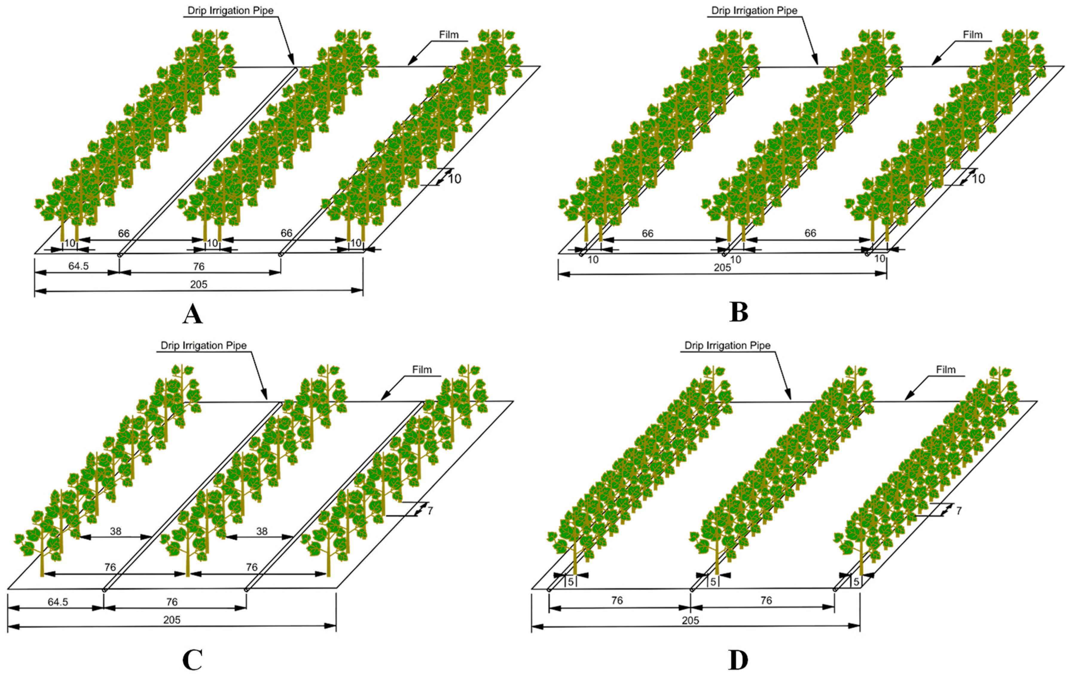
Three experiments were conducted (Figure 1 and

Table 1. Sampling date and corresponding growing seasons for the ground-measured leaf area index (LAI) and unmanned aerial vehicle (UAV) missions in three experiments.

Experiment	Year	Samples	Sensing and Sampling Date	Period
Experiment A	2021	51	3 June 20 June 13 July 3 August 28 August	Budding Late budding Flowering Boll forming Boll opening
Experiment B	2021	24	11 June 26 July 7 August 5 September	Budding Flowering Boll forming Boll opening
Experiment C	2020	27	26 July 12 August 4 September	Flowering Boll forming Boll opening

There were only 3 valid samples in the last sampling of experiment A, due to the lodging phenomenon that occurred.

). We studied drip-irrigated cotton growing under a 2.05-m-thick film. In experiment A (2021), the cotton variety used was Zhongmian 113. Four planting modes (Figure 2) and three irrigation quota (300 mm, 375 mm and 450 mm) were used. In experiment B (2021), the cotton variety used was Zhongmian 40. One planting mode was used: one film, two drips and six rows, with two irrigation rates (300 mm and 450 mm) and three salt treatments (0.2%, 0.4% and 0.6%) were studied. In experiment C (2020), the cotton variety used was Xinluzhong 47. The single planting mode was one film, two drips and six rows, with three irrigation rates (300 mm, 375 mm and 450 mm) and three salt treatments (0.2%, 0.4% and 0.6%). Other agronomic management was identical in each experiment. The data from experiment A were used for modeling verification, while the data from experiments B and C were used to test the model robustness and generalizability.

Experiment plots were arranged in a split plot design. We randomly selected a 2.05 m² (2.05 × 1) plot in each cell as the actual measurement quadrat, recording the fixed position with a GPS instrument (Garmin Corporation, USA). A SunScan (Delta-T, UK) was used to measure LAI in a cotton quadrat, with measurements taken at noon (14:00 Beijing time).

2.2. UAV Data Acquisition

UAV sensor (two DJI Matrice 600 Pro UAV, DJI, China) data were acquired after the ground LAI values were measured (Figure 3). Multispectral data were acquired using a RedEdge-M multispectral camera (MicaSense, USA) containing five bands—475 nm (blue), 560 nm (green), 668 nm (red), 717 nm (red edge) and 840 nm (NIR), with a focal length of 5.5 mm, a field angle of view of 47.2° and a resolution of 1280 × 960 pixels. The camera was equipped with a radiometric calibration plate that converted multispectral images into reflectance images; calibration was performed before each flight. GS Pro (DJI, China) software was used to plan the route and set the heading and side overlap rate (87%) and flight height (70 m). Flight speed was held constant at 4 m/s, and the lens was oriented vertically downward when shooting with a resolution of 5 cm/pixel.

LiDAR data were acquired using the LiAir 200 system (Green Valley, China) after the multispectral data acquisition was complete. With this instrument, the laser wavelength was 903 nm, the vertical angular resolution was 0.33°, the horizontal angular resolution was 0.2°, the scanning frequency was 10HZ and the maximum effective measurement rate was 720,000 Pts/sec. GS Pro software was also used for route planning, setting the heading and side overlap rate (80%), flight height (50 m) and flight speed (5 m/s).

2.3. UAV Data Preprocessing

2.3.1. Multispectral Data Preprocessing

Multispectral data were processed using the agricultural multispectral module in a Pix4D mapper (Pix4D SA, Switzerland). The solar radiation information collected by the sensor module on the top of the UAV and the standard reflectance values of each band taken by the radiation calibration plate were used for radiation calibration. Calibrated images were spliced to obtain the reflectance images of each band from the test site.

Sixteen common VIs were selected in this study, and the VI maps of the test site were obtained through band operation. Calculation formulas are shown in

Table 2. Definition and calculation formula of the selected vegetation indices (VIs) in this study.

VIs	Name	Formula	Reference
GI	Green–Red Ratio Index	G/R	[31]
RVI	Ratio ChlorophyII Vegetation Index	NIR/R	[32]
CVI	ChlorophyII Vegetation Index	(NIR × R)/(G2)	[33]
GLI	Green Leaf Index	(2G − R − B)/(2G + R + B)	[34]
CIRE	ChlorophyII Index—RedEdge	NIR/RE − 1	[35]
CIG	ChlorophyII Index—Green	NIR/G − 1	[35]
NDVI	Normalized Difference Vegetation Index	(NIR − R)/(NIR + R)	[36]
GNDVI	Green Normalized Difference Vegetation Index	(NIR − G)/(NIR + G)	[37]
NDREI	Normalized Difference Red Edge Index	(NIR − RE)/(NIR + RE)	[38]
EVI	Enhanced Vegetation Index	2.5(NIR − R)/(NIR + 6R − 7.5B + 1)	[39]
EVI2	Enhanced Vegetation Index Without A Blue Band	2.5(NIR − R)/(NIR + 2.4R + 1)	[40]
SAVI	Soil Adjusted Vegetation Index	1.5(NIR − R)/(NIR + R + 0.5)	[41]
OSAVI	Optimized Soil Adjusted Vegetation Index	1.16(NIR − R)/(NIR + R + 0.16)	[42]
NDGI	Normalized Difference Greenness Vegetation	(G − R)/(G + R)	[43]
MTCI	MERIS Terrestrial Chlorophyll Index	(NIR − RE)/(RE − R)	[44]
MCARI	Modified Chlorophyll Absorption in Reflectance Index	((RE − R) − 0.2(RE − G))(RE/R)	[45]

. Using the quadrat GPS information, the corresponding 16 VIs were accurately extracted from the vegetation index map for the subsequent analysis.

2.3.2. LiDAR Data Preprocessing

LiDAR360 software (Green Valley, China) were used to process and analyze the point cloud data. The high/low gross noise of the original point cloud were first removed, followed by dividing the point cloud into ground and vegetation points based on slope filtering and an irregular triangulation algorithm. Ground points were used to normalize the LiDAR data.

LiDAR can be used to extract a wide range of plant structural attributes, such as height, stem diameter and canopy density. One hundred structural parameters were extracted from the normalized LiDAR point cloud and created as raster bands. Then, all datasets were resampled to a spatial resolution of 5 cm for the model establishment and data fusion. The elevation parameters (including Elev_max, Elev_mean, Elev_stddev, etc.) directly reflect the distribution of the cotton canopy in each sample, which are calculated by aggregating the elevation statistics of all raster cells in the sample. The intensity parameter reflects the reflectance and surface composition of the cotton to distinguish differences within the canopy (leaves, branches, and bolls), also obtained by statistical aggregation of the raster cells, while the density parameters reflect the internal structure of the cotton canopy, with detailed definitions of each parameter in the table (Table S1). The structural parameters derived from point cloud data are used as input parameters for the model, and the overall shape and structural characteristics of cotton can be obtained by analyzing the statistics of raster within the sample.

2.4. LAI Model Development

2.4.1. Empirical Statistical Regression Model Development

We used Origin 2021b software (OriginLab, USA) to screen the feature parameters. Pearson’s correlation analysis was conducted between the measured LAI and corresponding VIs and structural parameters using the correlation plot package. The sensitive feature parameters with highly significant correlations were screened out. We reduced the dimension of the sensitive feature parameters using the Principal Component Analysis and extracted the top three sensitive feature parameters with their contribution rate.

The feature parameters selected above were used to build optimal LAI models with different empirical statistical regression modeling methods. The models include linear function (Equation (1)), exponential function (Equation (2)), logarithmic function (Equation (3)), power function (Equation (4)) and multiple linear regression (Equation (5)).

$$LAI=aX+b$$

(1)

$$LAI=a{e}^X$$

(2)

$$LAI=aln\left(X\right)+b$$

(3)

$$LAI=a{X}^b$$

(4)

$$LAI=a_1{X}_1+a_2{X}_2+a_3{X}_3+a_4{X}_4+\dots \dots +a_n{X}_n+b$$

(5)

where X, X₁, X₂, ……, X_n were the model input parameters.

2.4.2. Machine Learning Model Development

Random Forest Regression (RFR), Support Vector Regression (SVR) and Artificial Neural Network (ANN) were used in this study, because they can handle high-dimensional datasets and have been successful in estimating LAI [46,47]. We compared the potential of multispectral, LiDAR and fused two sensor data in estimating LAI by analyzing spectral parameters, structural parameters and multisource parameters as input feature quantities for each machine learning model. Python Scikit-learn was used to build the LAI machine learning model.

RFR is a nonlinear integrated modeling approach based on multiple decision trees, which can evaluate the importance of input parameters and partially handle the multi-collinearity between these variables while showing an excellent tolerance for outliers and noise. N_Estimators were iterated at the model training stage, where the parameters were set from 1 to 1000 with increments of 50, and the optimal parameters were determined by k-fold cross-validation.

SVR is a powerful machine learning algorithm based on a supervised learning model with user-defined kernel functions and optimization parameters that construct the optimal hyperplane in n-dimensional space and construct a regression by minimizing the distance between data points in the training set and the hyperplane. In this study, the Gaussian Radial Basis Function (RBF) was used as the kernel function. The C parameter acts as the degree of tolerance when searching for the decision function, and the optimized C value was set from 1 to 50 with increments of 1. The gamma parameter reflects the weight of the input parameters and selects from 0.001 to 0.5 with increments of 0.0005. Both gamma and C were iteratively adjusted at the model training stage.

ANN is a mathematical model inspired by the structure and behavior of the human brain. The architecture of ANN minimizes the mean square bias by error correction learning rules while adjusting the weights of each layer of neurons to reduce errors. It is often used to deal with complex nonlinear relationships between canopy spectral and phenotypic parameters with higher accuracy but lower model interpretability. In this study, the model accuracy is evaluated according to different input feature parameters with a different number of hidden layers and transmission algorithms to determine the best configuration of ANN. Finally, a single hidden layer based on the backpropagation algorithm was selected. The number of neurons in the hidden layer adjusted according to the characteristic number of input samples.

2.4.3. Gap Fraction Model Development

The theoretical basis of the physical model for estimating LAI based on the correlation of gap fractions is the Beer–Lambert law (Equation (6)). LiDAR cannot measure the gap fraction directly, but the LAI can be estimated by analyzing the correlation between the actively emitted laser data and the gap fraction. The LiDAR system used in this study can estimate the gap fraction by counting the number or intensity of the point cloud while using the extinction coefficient instead of the light attenuation phenomenon within the canopy [16]. However, it was found that the intensity-based ratio information is noisier and less stable than the number-based ratio information, and then, the calculation formula was modified as follows (Equation (7)):

$$P(\theta )=e^{-G\left(\theta \right)·LAI/\cos \theta }$$

(6)

$$LAI=-\frac{\cos \left(ang\right)}{\mathrm{k}}\times \ln \left(\frac{n_{ground}}{n_{all}}\right)$$

(7)

where P(θ) is the canopy gap fraction when the zenith angle is θ, k is the extinction coefficient, ang is the average scanning angle and n_ground and n_all are the ground and total points of the calculation grid.

To maximize the light energy utilization for photosynthesis, leaves in the cotton canopy grow in a radial direction, and the overall leaf inclination angle is approximately spherical in space [48]. Therefore, in this study, we set extinction coefficient k as 0.5. We chose 5 computational grid cell pixels (10 cm, 20 cm, 50 cm, 100 cm and 200 cm) and resampled the calculation results at 5 cm. The LAI estimation value was counted with pixel values of the sample. Considering the extreme value phenomenon that may occur with a low number of ground echoes, the LAI_max value of local cotton from different periods was used as the calculation threshold (

Table 3. Thresholds limit at various periods of cotton used for model correction in this study.

Period	LAImax
Budding	2
Late budding	3
Flowering	5
Boll-forming	7
Boll-opening	6

).

2.5. Statistical Analysis and Validation

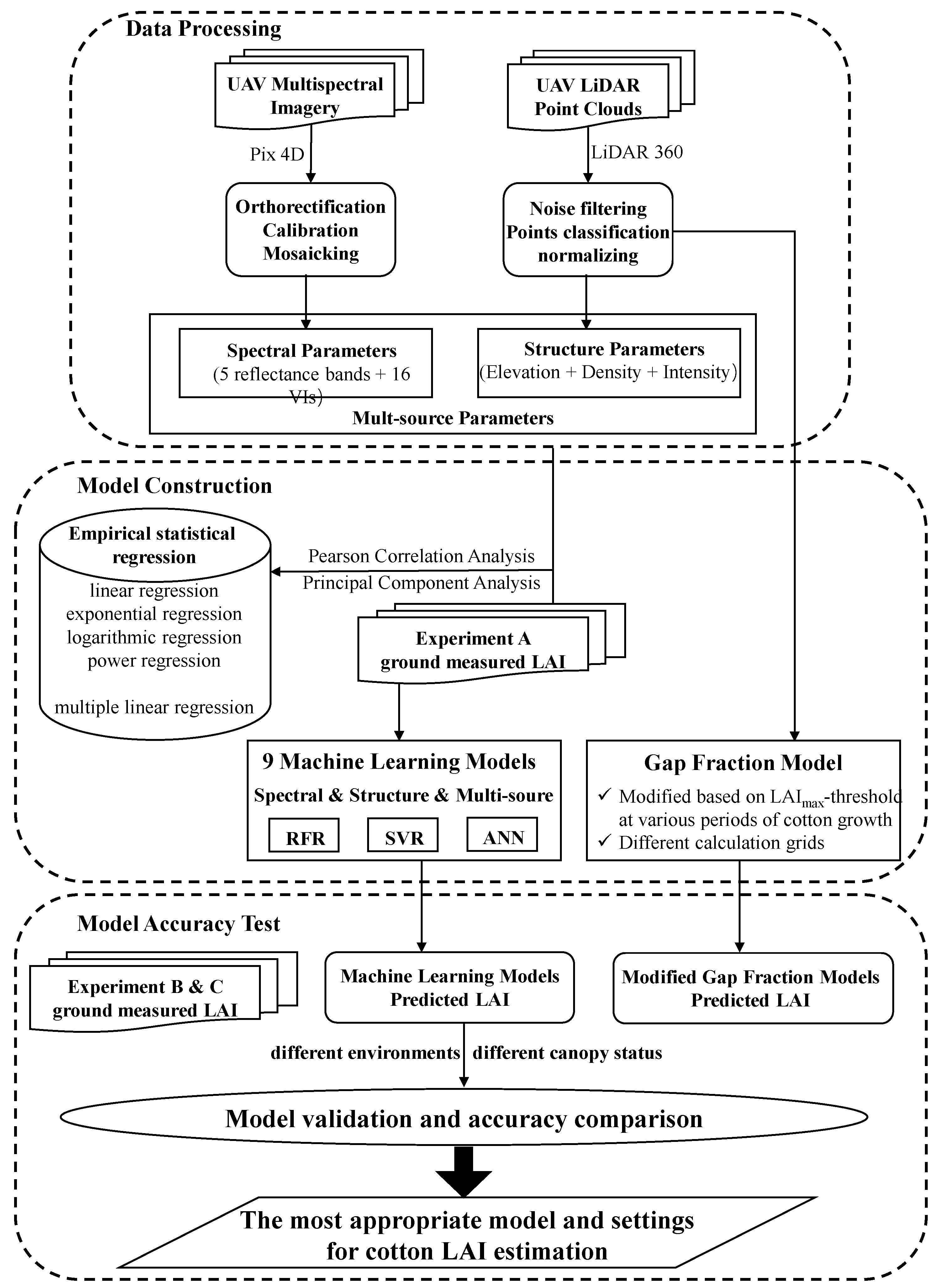
The procedure of statistical analysis after data collection was shown in the flowchart (Figure 4). There were 51 valid samples in experiment A. The method of cross-validation was used for resampling, where 70% of the data was used as the training set (n = 36). The remaining 30% were used as the validation set (n = 15). The statistical regression model was constructed based on sensitive parameters filtered by a correlation analysis between spectral/structural parameters and measured LAI, while machine learning models were constructed and adjusted by using training sets of all the spectral parameters, all structural parameters and multisource parameters as the input feature parameters, respectively. Model accuracy was evaluated by the coefficient of determination (R², Equation (8)) and root mean square error (RMSE, Equation (9)) in the validation dataset. Experiment B (different plots, n = 24) and experiment C (different years, n = 27) were used to test the model robustness and generality. In addition, normalized root mean square error (NRMSE, Equation (10)) was introduced to eliminate LAI dimension differences among experiments.

$$R^2=1-\frac{{\sum }_{i=1}^{\mathrm{n}}{\left(y_i-{\widehat{y}}_i\right)}^2}{{\sum }_{i=1}^{\mathrm{n}}{\left(y_i-{\overline{y}}_i\right)}^2}$$

(8)

$$RMSE=\sqrt{\frac{1}{n}{{\displaystyle \sum }}_{i=1}^{\mathrm{n}}{\left(y_i-{\widehat{y}}_i\right)}^2}$$

(9)

$$NRMSE=\frac{RMSE}{{\overline{y}}_i}\ast 100\%$$

(10)

where ŷ_i and y_i are estimated, ground measured cotton LAI, $\overline{y}$ is the mean value of ground measured LAI and n is the number of samples.

3. Results

3.1. Variation in Ground-Measured LAI

There were differences in the spectral reflectance between the soil and cotton canopy (Figure 5), where the soil and cotton canopy showed large differences in the red edge and NIR bands, which can be used to effectively reduce the noise interference of soil within the mixed image. At the same time, the canopy spectral reflectance of cotton in the three experiments was affected by different growth environments, with experiment A showing higher spectral reflectance in all bands and experiment B showing higher values in the RGB band than experiment C. The measured LAI of cotton in each experiment showed a trend of rapid increase in the early period and a slight decrease in the subsequent period, while there were differences in the structure of cotton affected by different growth environments in the three experiments (Figure 6). The LAI in experiment A used for modeling was concentrated in the range of 0.12–6.02. Cotton in experiment B was affected by salt stress, resulting in lower LAI values (0.64–3.68). On the contrary, the LAI values showed high levels (2.6–5.52) in experiment C because of the sufficient light and heat resources in 2020. However, the LAI showed large variability in different periods, making the training set covers most of the possible scenarios of the LAI values. Thus, testing the model robustness using experiments B and C data is necessary and meaningful.

3.2. Model Development

We found a very significant negative correlation with LAI in blue, green and red bands and a very significant positive correlation in the NIR band (Figure 7 and Figure 8). The VIs also showed very significant positive correlations with LAI, except GI, GLI and NDGI—among which, CVI, CIRE, CIG and NDREI had higher correlations (Figure 7). Height parameters were more highly correlated than the intensity and density parameters—among which, Elev_AIH_5th, Elev_20th, Elev_sqrt_mean_sq and Elev_mean all had higher correlations (Figure 8). PCA was used to dimensionally reduce the spectral, structural and multisource parameters; spectral parameters (CIRE, GNDVI and MTCI); structural parameters (Elev_AIH_5th, Elev_sqrt_mean_sq and Coverage) and multisource parameters (Elev_AIH_5th, GNDVI and MTCI), all screened for multiple statistical regression modeling.

We calculated the accuracy based on the statistical regression models (

Table 4. Quantitative relationship between the LAI and measured values based on statistical regression models in experiment A.

Input Dataset	Feature Index	Model	Equation	R2	RMSE
Spectral	CVI	Power	y = 0.148X1.849	0.810	1.100
	CIRE	Exponential	y = 0.399e1.323X	0.824	1.056
	CIG	Exponential	y = 0.446e0.350X	0.791	1.667
	NDREI	Exponential	y = 0.211e6.239X	0.839	0.923
	CIRE/GNDVI /MTCI	multivariate linear	y = 2.973X1 − 2.762X2 + 0.357X3 − 0.081	0.787	1.130
Structure	Elve_AIH_5th	Power	y = 22.874X1.162	0.822	1.756
	Elve_20th	Power	y = 16.883X1.116	0.816	1.767
	Elve_sqrt_mean_sq	Power	y = 10.697X1.111	0.821	1.745
	Elve_mean	Power	y = 11.356X1.113	0.821	1.746
	Coverage/Elve_AIH_5th /Elve _sqrt_mean_sq	multivariate linear	y = 4.912X1 + 16.88X2 − 10.414X3 − 0.249	0.760	1.573
Multisource	Elve _AIH_5th/GNDVI/ MTCI	multivariate linear	y = 7.659X1 + 2.067X2 + 1.477X3 − 2.858	0.823	1.212

). The R² of the models ranged from 0.76 to 0.84, and the RMSE values were 0.923–1.767. Nonlinear models had higher accuracy than the multivariate linear regression models. Among the nonlinear models, the exponential function model based on spectral parameters performed best, while the structural parameter model had the highest accuracy with the power function model. Although the fusion of multisource data had the advantage of different sensors, it was affected by the model structure of the model, and multiple linear regression was ineffective at estimating the cotton LAI.

The multisource parameters performed better among three machine learning algorithms, with the best performance based on the RFR algorithm (R² = 0.950, RMSE = 0.332,

Table 5. Quantitative relationship between the LAI and measured values based on the machine learning models in experiment A.

Model	Input Dataset	Feature	Parameter Settings	R2	RMSE	NRMSE
RFR	Spectral	21	Tree = 200	0.886	0.531	22.3%
	Structure	100	Tree = 300	0.630	0.960	40.3%
	Multisource	121	Tree = 500	0.950	0.332	13.9%
SVR	Spectral	21	C = 4/Gamma = 0.03	0.889	0.524	22.0%
	Structure	100	C = 2/Gamma = 0.0015	0.645	0.939	39.5%
	Multisource	121	C = 8/Gamma = 0.01	0.843	0.504	21.2%
ANN	Spectral	21	Layer size = 5	0.850	0.608	25.5%
	Structure	100	Layer size = 15	0.550	1.099	46.2%
	Multisource	121	Layer size = 30	0.848	0.503	21.1%

). The structural parameter model was slightly less accurate than the other models.

LAI estimation of the gap fraction model modified based on the LAI_max threshold at various periods of cotton had a high estimation accuracy (the slope of the fitting equation was close to 1, higher R² and lower RMSE, Figure 9). For different-sized calculation grids, the estimation accuracy first increases and then decreases with improvements in the spatial resolution. High-resolution grids (10 cm, 20 cm and 50 cm) performed with higher accuracy compared to lower-resolution grids (100 cm and 200 cm); the 20-cm grid performed the best (R² = 0.953, RMSE = 0.378), and the 200-cm grid performed the worst (R² = 0.814, RMSE = 0.786).

Both statistical regression and machine learning showed an excellent fit for modeling cotton LAI. However, the RMSE of the machine learning model was much lower than the statistical regression model (RMSE_min of machine learning = 0.332 and RMSE_min of statistical regression = 0.923). This indicated that the machine learning model could more accurately reflect the true cotton LAI. Therefore, only the machine learning model estimation results were analyzed in the subsequent testing set, and for the modified gap fraction model, only the 10, 20 and 50 cm grid resolution results were analyzed.

3.3. Model Accuracy Assessment Using

When only the spectral parameters were input, all three machine learning algorithms performed poorly (R²: 0.102–0.167, NRMSE: 58.9–60.4%,

Table 6. Quantitative relationship between the LAI and measured values based on the machine learning models in test dataset (experiments B and C).

Input Dataset	Feature Index	Test Dataset
		Equation	R2	RMSE	NRMSE
Spectral	RFR	Y = 0.12X + 1.558	0.167	1.793	56.9%
	SVR	Y = 0.081X + 1.638	0.102	1.855	58.9%
	ANN	Y = 0.132X + 1.402	0.111	1.902	60.4%
Structure	RFR	Y = 0.748X + 0.096	0.76	0.992	31.5%
	SVR	Y = 0.675X + 0.077	0.848	1.132	35.9%
	ANN	Y = 1.02X − 0.39	0.751	0.905	28.7%
Multisource	RFR	Y = 0.593X + 0.566	0.835	0.998	31.7%
	SVR	Y = 0.553X + 0.978	0.665	0.955	30.3%
	ANN	Y = 1.001X + 0.382	0.746	0.923	29.3%

). The structural and multisource parameters exhibited different accuracies under different machine learning models (Table 6), whereas the RFR model performed better when importing multisource parameters (R² = 0.835). The accuracy of the SVR model decreased when the fusion multisource parameters (R² = 0.665) and the ANN model were reasonably accurate, with two different input parameters (structural parameters: R² = 0.751, NRMSE = 28.7% and multisource parameters: R² = 0.746, NRMSE = 29.3%).

In order to obtain the reasons for the degradation of the model accuracy in the test set, further analysis of the LAI estimation results based on machine learning models before and after cotton canopy closure was carried out (

Table 7. Quantitative relationship between the LAI and measured values based on machine learning models before and after canopy closure in the test dataset (experiments B and C).

Input Dataset	Feature Index	Before Canopy Closure				After Canopy Closure
		Equation	R2	RMSE	NRMSE	Equation	R2	RMSE	NRMSE
Spectral	RFR	Y = 0.104X + 1.59	0.242	1.261	59.5%	Y = 0.137X + 1.495	0.081	2.086	53.9%
	SVR	Y = 0.052X + 1.712	0.439	1.305	61.5%	Y = 0.134X + 1.424	0.084	2.158	55.7%
	ANN	Y = 0.086X + 1.561	0.075	1.341	63.2%	Y = 0.266X + 0.839	0.167	2.211	57.1%
Structure	RFR	Y = 0.668X + 0.4	0.680	0.815	38.4%	Y = 1.018X − 1.046	0.801	1.099	28.4%
	SVR	Y = 0.607X + 0.334	0.853	0.798	37.6%	Y = 0.903X − 0.887	0.857	1.317	34.0%
	ANN	Y = 0.649X + 0.128	0.645	1.006	47.4%	Y = 1.158X − 0.741	0.672	0.827	21.3%
Multisource	RFR	Y = 0.529X + 0.703	0.969	0.707	33.3%	Y = 0.676X + 0.245	0.670	1.159	29.9%
	SVR	Y = 0.401X + 1.424	0.751	0.872	41.1%	Y = 0.902X − 0.459	0.724	1.009	26.1%
	ANN	Y = 0.67X + 0.702	0.848	0.581	27.4%	Y = 0.946X + 0.861	0.530	1.100	28.4%

and Figure 10). The accuracy of RFR is higher than SVR and ANN in machine learning models. However, the model accuracy for different canopy conditions is related to the input parameters. In this study, for example, RFR based on multisource parameters before canopy closure has a higher accuracy, while RFR based on structural parameters performs better after canopy closure. Machine learning models based on RFR and SVR have a higher fitting accuracy before canopy closure than after closure with the spectral parameters input. However, models based on the structural parameters were more accurate after canopy closure. Multisource parameters that fused spectral and structural parameters could improve the accuracy of the RFR model and ANN model before canopy closure, but the accuracy declined relative to that of the structural parameter model after canopy closure, while the accuracy of the SVR model did not change significantly before and after canopy closure.

Estimation of the test dataset based on the modified gap fraction model was more accurate (R² above 0.9) than the machine learning models (

Table 8. Quantitative relationships between the LAI and measured values with different calculation grids based on the modified gap fraction model before and after canopy closure in the test dataset (experiments B and C) based on the maximum threshold modified porosity model.

Feature Index	Test Dataset
	R2	RMSE	NRMSE
10 cm	0.948	0.338	10.7%
20 cm	0.955	0.319	10.1%
50 cm	0.902	0.457	14.5%

). The model accuracy was consistent with the modeling set under different calculation grid sizes, where the 20-cm grid also performed best (R² = 0.955, NRMSE = 10.1%).

4. Discussion

4.1. Parameter Performance and Comparison of Different Models

We performed sensitivity screening for 16 commonly used VIs and found that the empirical statistical model based on NDREI had the highest accuracy in estimating LAI [49]. Although CVI, CIRE and CIG among the VIs were more correlated with LAI (Figure 7), studies have shown that red edge bands (680–760 nm) were sensitive to LAI [50], and the NIR band (780–1100 nm) could be used to distinguish plant leaves from other tissues [51,52]. In this study, the NIR reflectance value of cotton canopy showed a significant positive correlation with LAI (Figure 7), while the reflectance value of the soil and cotton canopy showed large differences in the red edge and NIR bands (Figure 5), NDREI was calculated based on the normalized difference between the NIR and red edge bands, which increased the differences between leaves and soil and could effectively remove the influence of soil noise within the mixed image. One hundred structural parameters were based on LiDAR, where the elevation parameters were better correlated than the intensity/density parameters in this study (Figure 8) [25]. That is because cotton has thinner stalks and a larger leaf area ratio than other crops, and the intensity parameter is unsuitable for estimating the LAI alone. In order to maximize light energy utilization for photosynthesis, the leaves in the canopy will grow in the surrounding direction, and the leaves inside the canopy are relatively small, so the relationship between the density parameter and LAI is relatively weak. The elevation parameters, especially elevation percentile, were extremely strongly and positively correlated with LAI, because they accurately represent the structural distribution of different crop heights, and there is a direct significant correlation between plant height and leaf area [53]. Meanwhile, the cotton structure resembles a trapezoid [54], and more information is contained in the relatively low position of the canopy. Thus, the empirical statistical regression model based on Elev_AIH_5th has a higher accuracy than other structural parameters in the LAI estimation.

For the statistical regression models, LAI and spectral/structural parameters have a nonlinear relationship that is determined by the physiological characteristics of cotton [55,56]. Although the nonlinear empirical statistical regression model based on sensitive parameters can simulate the trend between parameters and LAI, the absolute deviation of the LAI estimates from the measured values is large, which shows that the nonlinear relationship and suitable input parameters cannot fully explain the growth pattern of cotton LAI. On the contrary, machine learning models focus on mining the intrinsic connection between input parameters and LAI without focusing on the mathematical quantitative formula of the model in this study. The input parameters are where a variety of spectral information allows for a complete presentation of the optical information of the LAI, the elevation parameters reflect the distribution directly, the intensity parameter reflects the surface composition and the density parameters reflect the internal structure. Optimizing the model structure by adjusting the combination of input parameters theoretically solves the multicollinearity problem of predictors. At the same time, there are many uncertainties in cotton under different growth environments, and the modeling framework of simple empirical statistics cannot handle the effect of noise. Due to the powerful ability to fuse data and handle noise, the machine learning models performed with higher accuracy than the statistical regression models in estimating LAI.

4.2. Verification of the Universality of Machine Learning Models

The accuracy of machine learning models for estimating LAI decreased in the test datasets. This was because machine learning models only learn from known samples and interpret the results based on statistical knowledge. Therefore, their application was only valid in calibrated regions [57]. The growth pattern of cotton is different under different space–time conditions, with consequent changes in the canopy spectral reflectance and structure, which leads to a decrease in the estimation accuracy of the machine learning model in the tested dataset. Thus, it is important and necessary to test the robustness of the model using cotton data sets from different growth environments. In this study, the machine learning models were tested using data from cotton in different plots and years, where the structure and canopy spectral reflectance of cotton was affected by the environment (Figure 5 and Figure 6). The accuracy of machine learning models based on spectral parameters decreased most [58,59]. However, the machine learning model based on structural parameters is closely related to the growth pattern of cotton, whose intrinsic relationship was less affected by structural changes, although the estimation accuracy is decreased in the test data but is still acceptable. The accuracy of the RFR model fused with multisource parameters was higher than that of spectral or structural parameters, because this method did not need to perform feature selection when processing multi-feature data. Instead, it performs weight distribution modeling based on the input parameters, which improves the fitting accuracy as the input parameters increase [60]. In this study, the weight of the structural parameters of the RFR model based on multiple source parameters is large, and the LAI is estimated more accurately by obtaining beneficial spectral information when stabilizing the model variation trend. The SVR eliminates feature information when finding the most suitable hyperplane fit data by SG smoothing and noise reduction, which is influenced by the input parameters and Cost (C) [9,19]. This study sets a high Cost (C = 8), and with the increase of the input parameters, the eliminated information also increases, leading to a decrease in the model accuracy. Although the accuracy of the ANN estimation improves with increasing the input parameters, the limited boosting, lower training efficiency and the need for a larger input sample size [60,61] limit its application in estimating cotton LAI.

Selecting the appropriate input parameters for different canopy opening and closing statuses can alleviate the degradation of accuracy in this study, where input parameters select multisource parameters before canopy closure while structural parameters are selected after canopy closure. Since the applicability of the two sensors before and after canopy closure is different, the canopy of cotton is small before the canopy closure, and LiDAR obtains less cotton point cloud data and more soil point clouds, whose noise disturbs the estimation accuracy of the machine learning model based on the structural parameters; at this time, using the spectral characteristics can accurately separate the features, and fusion spectral and the structural parameters can effectively improve the accuracy of the LAI estimation. LiDAR can accurately obtain canopy and internal information by actively emitting laser light that penetrates the canopy after canopy closure. The machine learning models based on structural parameters estimate cotton LAI with a high accuracy. However, the spectral is limited by the light saturation problem to estimate the canopy physiological parameters [62]; once fused, the spectral parameters estimate the cotton LAI accuracy decrease instead.

4.3. Parameter Determination for the Gap Fraction Model

The LAI accuracy estimated by the gap fraction model was affected by the proportion of vegetation points and the calculation scale effect. The former was primarily related to observation equipment and data processing. In this study, the flight parameters were adjusted to suit the situation at the study site, and weeds in plots were removed through field management measures to eliminate the influence of spectral noise. At the same time, slope filtering and irregular triangular network encryption algorithms [63] were used to divide the point cloud into ground points and non-ground points. Finally, combined with the growth pattern of cotton, a height threshold of 5 cm was set when the crop growth was small and fixed to 10 cm after the budding period to separate the vegetation and ground point clouds. This enabled us to accurately calculate the proportion of vegetation point clouds.

The scale effect was caused by the nonuniformity in the spatial distribution of cotton leaves and nonlinearity of the inversion function [64]. Reducing the scale effect impacts by choosing a suitable computational grid is crucial for the accurate estimation of cotton LAI. Owing to plant spacing [28] and for other reasons, a large calculation grid is usually set in forestry. In this study, the quadrat was 2.05 m². If the calculation grid is too large, the size of the open space would not match and lead to inaccurate calculations. Therefore, we set the minimum and maximum grid sizes at 10 cm (plant spacing) and 200 cm (ground quadrat), and five computing units of 20 cm, 50 cm and 100 cm were added for analysis. We estimated the LAI with nine different grids in advance (10 cm, 15 cm, 20 cm, 25 cm, 30 cm, 35 cm, 40 cm, 45 cm and 50 cm). The estimation accuracy showed an overall trend of increasing and then decreasing, with 20 cm performing the best and maintaining a very high level of accuracy. We used 20 cm in this study as the most representative parameter. At the same time, the continuing resolution was not calculated, because the difference in accuracy between 5-cm steps was not obvious, and there would be some systematic and noise errors if smaller steps were used. However, the dense planting of cotton may maximize the value in some calculation grids and affect the estimation results. Using the LAI_max of cotton in each period as the grid threshold can effectively solve this problem. Since the growth pattern of cotton LAI was not the same in different periods, which was particularly necessary to set thresholds for each period. To maximize the light energy utilization for photosynthesis leaves in the cotton canopy growth in a radial direction, the overall leaf inclination angle is approximately spherical in space [48]. Therefore, it can be assumed that the leaf distribution is homogeneous within each raster. Using the maximum LAI at each reproductive stage as the threshold can simulate its real situation while reducing the noise and scale effects.

We did not explore the specific deviation induced by scale effects in this study but presented a method to modify the model based on the LAI_max threshold at various periods of cotton growth. From this, we analyzed the LAI estimation accuracy under different grid sizes. The accuracy was highest when the calculation grid was set to 20 cm, which might be due to cotton morphology and the effect of the growth height. Usually, researchers adjusted the scale according to indicators from the research object to obtain more comprehensive ground vegetation information. In such cases, taller trees with larger unit canopies were used to obtain information at low resolutions [65,66,67], while low herbs required higher resolutions for more comprehensive information [68]; cotton was in between. In addition, there were almost no pure ground pixels in the 20-cm calculation grid. At the same time, for the areas with a low point cloud penetration rate caused by leaf occlusion in the quadrat, the influence of the maximum value could be effectively avoided by applying the upper threshold value. Therefore, the choice of a 20-cm resolution was the most suitable.

5. Conclusions

We used an UAV equipped with multispectral cameras and LiDAR to obtain cotton remote sensing data to find a method to accurately estimate cotton LAI. Our results showed that, in addition to the traditional spectral parameters, it is also feasible to estimate LAI using UAVs with LiDAR to obtain the structural parameters. Machine learning models, especially the RFR model, can estimate cotton LAI more accurately than empirical statistical regression models. When datasets from different environments are used to test the universality of the model, the overall accuracy of the machine learning model decreases. However, the estimated accuracy of the model, except for the model based on the spectral, remains within an acceptable range. Meanwhile, selecting appropriate input parameters for different canopy opening and closing statuses can alleviate accuracy degradation. For example, this study selects multisource parameters as input parameters before canopy closure and structural parameters after canopy closure. Finally, we propose a gap fraction model based on a LAI_max threshold at various periods of cotton growth, which can estimate cotton LAI with a high accuracy, particularly when the calculation grid is 20 cm (R² = 0.952, NRMSE = 12.6%). This method does not require much data modeling and has a strong universality, but it is essential to press the LAI_max threshold of the crop for reducing the noise and select the most appropriate computational grids. The two suitable settings may also vary among crops, and future study is required.

References

- Chen, J.M.; Black, T.A. Defining Leaf Area Index for Non-Flat Leaves. Plant Cell Environ. 1992, 15, 421–429. [Google Scholar] [CrossRef]
- BUNCE, J.A. Growth Rate, Photosynthesis and Respiration in Relation to Leaf Area Index. Ann. Bot. 1989, 63, 459–463. [Google Scholar] [CrossRef]
- Chen, J.M.; Rich, P.M.; Gower, S.T.; Norman, J.M.; Plummer, S. Leaf Area Index of Boreal Forests: Theory, Techniques, and Measurements. J. Geophys. Res. Atmos. 1997, 102, 29429–29443. [Google Scholar] [CrossRef]
- Yao, Y.; Liu, Q.; Liu, Q.; Li, X. LAI Retrieval and Uncertainty Evaluations for Typical Row-Planted Crops at Different Growth Stages. Remote Sens. Environ. 2008, 112, 94–106. [Google Scholar] [CrossRef]
- Hill, M.J.; Senarath, U.; Lee, A.; Zeppel, M.; Nightingale, J.M.; Williams, R.D.J.; McVicar, T.R. Assessment of the MODIS LAI Product for Australian Ecosystems. Remote Sens. Environ. 2006, 101, 495–518. [Google Scholar] [CrossRef]
- Liu, J.; Pattey, E.; Jégo, G. Assessment of Vegetation Indices for Regional Crop Green LAI Estimation from Landsat Images over Multiple Growing Seasons. Remote Sens. Environ. 2012, 123, 347–358. [Google Scholar] [CrossRef]
- Zhang, Z.; Tang, B.-H. Estimation of Leaf Area Index with Various Vegetation Indices from Gaofen-5 Band Reflectances. In Proceedings of the IGARSS 2018—2018 IEEE International Geoscience and Remote Sensing Symposium, Valencia, Spain, 23–27 July 2018; pp. 2619–2622. [Google Scholar]
- von Bueren, S.; Burkart, A.; Hueni, A.; Rascher, U.; Tuohy, M.; Yule, I. Comparative Validation of UAV Based Sensors for the Use in Vegetation Monitoring. Biogeosci. Discuss. 2014, 11, 3837–3864. [Google Scholar] [CrossRef]
- Li, S.; Yuan, F.; Ata-UI-Karim, S.T.; Zheng, H.; Cheng, T.; Liu, X.; Tian, Y.; Zhu, Y.; Cao, W.; Cao, Q. Combining Color Indices and Textures of UAV-Based Digital Imagery for Rice LAI Estimation. Remote Sens. 2019, 11, 1763. [Google Scholar] [CrossRef]
- Hasan, U.; Sawut, M.; Chen, S. Estimating the Leaf Area Index of Winter Wheat Based on Unmanned Aerial Vehicle Rgb-Image Parameters. Sustainability 2019, 11, 6829. [Google Scholar] [CrossRef]
- Yao, X.; Wang, N.; Liu, Y.; Cheng, T.; Tian, Y.; Chen, Q.; Zhu, Y. Estimation of Wheat LAI at Middle to High Levels Using Unmanned Aerial Vehicle Narrowband Multispectral Imagery. Remote Sens. 2017, 9, 1304. [Google Scholar] [CrossRef] [Green Version]
- Yamaguchi, T.; Tanaka, Y.; Imachi, Y.; Yamashita, M.; Katsura, K. Feasibility of Combining Deep Learning and Rgb Images Obtained by Unmanned Aerial Vehicle for Leaf Area Index Estimation in Rice. Remote Sens. 2021, 13, 84. [Google Scholar] [CrossRef]
- Wang, Y.; Fang, H. Estimation of LAI with the LiDAR Technology: A Review. Remote Sens. 2020, 12, 3457. [Google Scholar] [CrossRef]
- Tunca, E.; Köksal, E.S.; Çetin, S.; Ekiz, N.M.; Balde, H. Yield and Leaf Area Index Estimations for Sunflower Plants Using Unmanned Aerial Vehicle Images. Environ. Monit. Assess. 2018, 190, 682. [Google Scholar] [CrossRef] [PubMed]
- Hu, T.; Sun, X.; Su, Y.; Guan, H.; Sun, Q.; Kelly, M.; Guo, Q. Development and Performance Evaluation of a Very Low-Cost UAV-LiDAR System for Forestry Applications. Remote Sens. 2021, 13, 77. [Google Scholar] [CrossRef]
- Richardson, J.J.; Moskal, L.M.; Kim, S.-H. Modeling Approaches to Estimate Effective Leaf Area Index from Aerial Discrete-Return LiDAR. Agric. For. Meteorol. 2009, 149, 1152–1160. [Google Scholar] [CrossRef]
- López-Calderón, M.J.; Estrada-Ávalos, J.; Rodríguez-Moreno, V.M.; Mauricio-Ruvalcaba, J.E.; Martínez-Sifuentes, A.R.; Delgado-Ramírez, G.; Miguel-Valle, E. Estimation of Total Nitrogen Content in Forage Maize (Zea Mays l.) Using Spectral Indices: Analysis by Random Forest. Agriculture 2020, 10, 451. [Google Scholar] [CrossRef]
- Singhal, G.; Bansod, B.; Mathew, L.; Goswami, J.; Choudhury, B.U.; Raju, P.L.N. Estimation of Leaf Chlorophyll Concentration in Turmeric (Curcuma Longa) Using High-Resolution Unmanned Aerial Vehicle Imagery Based on Kernel Ridge Regression. J. Indian Soc. Remote Sens. 2019, 47, 1111–1122. [Google Scholar] [CrossRef]
- Zhang, Z.; Masjedi, A.; Zhao, J.; Crawford, M.M. Prediction of Sorghum Biomass Based on Image Based Features Derived from Time Series of UAV Images. In Proceedings of the 2017 IEEE International Geoscience and Remote Sensing Symposium (IGARSS), Fort Worth, TX, USA, 23–28 July 2017; pp. 6154–6157. [Google Scholar]
- Cheng, Z.; Meng, J.; Shang, J.; Liu, J.; Huang, J.; Qiao, Y.; Qian, B.; Jing, Q.; Dong, T.; Yu, L. Generating Time-Series LAI Estimates of Maize Using Combined Methods Based on Multispectral UAV Observations and WOFOST Model. Sensors 2020, 20, 6006. [Google Scholar] [CrossRef]
- Qiao, L.; Gao, D.; Zhao, R.; Tang, W.; An, L.; Li, M.; Sun, H. Improving Estimation of LAI Dynamic by Fusion of Morphological and Vegetation Indices Based on UAV Imagery. Comput. Electron. Agric. 2022, 192, 106603. [Google Scholar] [CrossRef]
- De Almeida, D.R.A.; Broadbent, E.N.; Ferreira, M.P.; Meli, P.; Zambrano, A.M.A. Monitoring Restored Tropical Forest Diversity and Structure through UAV-Borne Hyperspectral and LiDAR Fusion. Remote Sens. Environ. 2021, 264, 112582. [Google Scholar] [CrossRef]
- Bork, E.W.; Su, J.G. Integrating LiDAR Data and Multispectral Imagery for Enhanced Classification of Rangeland Vegetation: A Meta Analysis. Remote Sens. Environ. 2007, 111, 11–24. [Google Scholar] [CrossRef]
- Luo, S.; Wang, C.; Pan, F.; Xi, X.; Li, G.; Nie, S.; Xia, S. Estimation of Wetland Vegetation Height and Leaf Area Index Using Airborne Laser Scanning Data. Ecol. Indic. 2015, 48, 550–559. [Google Scholar] [CrossRef]
- Luo, S.; Chen, J.M.; Wang, C.; Gonsamo, A.; Xi, X.; Lin, Y.; Qian, M.; Peng, D.; Nie, S.; Qin, H. Comparative Performances of Airborne LiDAR Height and Intensity Data for Leaf Area Index Estimation. IEEE J. Sel. Top. Appl. Earth Obs. Remote Sens. 2018, 11, 300–310. [Google Scholar] [CrossRef]
- Tang, H.; Brolly, M.; Zhao, F.; Strahler, A.H.; Schaaf, C.L.; Ganguly, S.; Zhang, G.; Dubayah, R. Deriving and Validating Leaf Area Index (LAI) at Multiple Spatial Scales through LiDAR Remote Sensing: A Case Study in Sierra National Forest, CA. Remote Sens. Environ. 2014, 143, 131–141. [Google Scholar] [CrossRef]
- Lang, A. Estimation of Leaf Area Index from Transmission of Direct Sunlight in Discontinuous Canopies. Agric. For. Meteorol. 1986, 37, 229–243. [Google Scholar] [CrossRef]
- Leblanc, S.G.; Chen, J.M.; Fernandes, R.; Deering, D.W.; Conley, A. Methodology Comparison for Canopy Structure Parameters Extraction from Digital Hemispherical Photography in Boreal Forests. Agric. For. Meteorol. 2005, 129, 187–207. [Google Scholar] [CrossRef]
- Pisek, J.; Lang, M.; Nilson, T.; Korhonen, L.; Karu, H. Comparison of Methods for Measuring Gap Size Distribution and Canopy Nonrandomness at Järvselja RAMI (RAdiation Transfer Model Intercomparison) Test Sites. Agric. For. Meteorol. 2011, 151, 365–377. [Google Scholar] [CrossRef]
- van Gardingen, P.R.; Jackson, G.E.; Hernandez-Daumas, S.; Russell, G.; Sharp, L. Leaf Area Index Estimates Obtained for Clumped Canopies Using Hemispherical Photography. Agric. For. Meteorol. 1999, 94, 243–257. [Google Scholar] [CrossRef]
- Zarco-Tejada, P.J.; Berjón, A.; López-Lozano, R.; Miller, J.R.; Martín, P.; Cachorro, V.; González, M.R.; de Frutos, A. Assessing Vineyard Condition with Hyperspectral Indices: Leaf and Canopy Reflectance Simulation in a Row-Structured Discontinuous Canopy. Remote Sens. Environ. 2005, 99, 271–287. [Google Scholar] [CrossRef]
- Pearson, R.L.; Miller, L.D. Remote Mapping of Standing Crop Biomass for Estimation of the Productivity of the Shortgrass Prairie. Remote Sens. Environ. 1972, VIII, 1355. [Google Scholar]
- Vincini, M.; Frazzi, E.; D’Alessio, P. A Broad-Band Leaf Chlorophyll Vegetation Index at the Canopy Scale. Precis. Agric. 2008, 9, 303–319. [Google Scholar] [CrossRef]
- Louhaichi, M.; Borman, M.M.; Johnson, D.E. Spatially Located Platform and Aerial Photography for Documentation of Grazing Impacts on Wheat. Geocarto Int. 2001, 16, 65–70. [Google Scholar] [CrossRef]
- Gitelson, A.A.; Gritz, Y.; Merzlyak, M.N. Relationships between Leaf Chlorophyll Content and Spectral Reflectance and Algorithms for Non-Destructive Chlorophyll Assessment in Higher Plant Leaves. J. Plant Physiol. 2003, 160, 271–282. [Google Scholar] [CrossRef] [PubMed]
- Rouse, J.W.; Haas, R.H.; Schell, J.A.; Deering, D.W. Monitoring the Vernal Advancement and Retrogradation (Greenwave Effect) of Natural Vegetation; NASA/GSFC Type III Final Report; NASA: Greenbelt, MD, USA; GSFC: Greenbelt, MD, USA, 1974.
- Gitelson, A.A.; Kaufman, Y.J.; Merzlyak, M.N. Use of a Green Channel in Remote Sensing of Global Vegetation from EOS-MODIS. Remote Sens. Environ. 1996, 58, 289–298. [Google Scholar] [CrossRef]
- Gitelson, A.; Merzlyak, M.N. Quantitative Estimation of Chlorophyll-a Using Reflectance Spectra: Experiments with Autumn Chestnut and Maple Leaves. J. Photochem. Photobiol. B Biol. 1994, 22, 247–252. [Google Scholar] [CrossRef]
- Huete, A.; Didan, K.; Miura, T.; Rodriguez, E.P.; Gao, X.; Ferreira, L.G. Overview of the Radiometric and Biophysical Performance of the MODIS Vegetation Indices. Remote Sens. Environ. 2002, 83, 195–213. [Google Scholar] [CrossRef]
- Jiang, Z.; Huete, A.R.; Didan, K.; Miura, T. Development of a Two-Band Enhanced Vegetation Index without a Blue Band. Remote Sens. Environ. 2008, 112, 3833–3845. [Google Scholar] [CrossRef]
- Huete, A.R. A Soil-Adjusted Vegetation Index (SAVI). Remote Sens. Environ. 1988, 25, 295–309. [Google Scholar] [CrossRef]
- Rondeaux, G.; Steven, M.; Baret, F. Optimization of Soil-Adjusted Vegetation Indices. Remote Sens. Environ. 1996, 55, 95–107. [Google Scholar] [CrossRef]
- Gamon, J.A.; Surfus, J.S. Assessing Leaf Pigment Content and Activity with a Reflectometer. New Phytol. 1999, 143, 105–117. [Google Scholar] [CrossRef]
- Dash, J.; Curran, P.J. The MERIS Terrestrial Chlorophyll Index. Int. J. Remote Sens. 2004, 25, 5403–5413. [Google Scholar] [CrossRef]
- Daughtry, C.S.T.; Walthall, C.L.; Kim, M.S.; de Colstoun, E.B.; McMurtrey, J.E. Estimating Corn Leaf Chlorophyll Concentration from Leaf and Canopy Reflectance. Remote Sens. Environ. 2000, 74, 229–239. [Google Scholar] [CrossRef]
- Liu, S.; Jin, X.; Nie, C.; Wang, S.; Yu, X.; Cheng, M.; Shao, M.; Wang, Z.; Tuohuti, N.; Bai, Y.; et al. Estimating Leaf Area Index Using Unmanned Aerial Vehicle Data: Shallow vs. Deep Machine Learning Algorithms. Plant Physiol. 2021, 187, 1551–1576. [Google Scholar] [CrossRef] [PubMed]
- Peng, Y.; Zhu, T.; Li, Y.; Dai, C.; Fang, S.; Gong, Y.; Wu, X.; Zhu, R.; Liu, K. Remote Prediction of Yield Based on LAI Estimation in Oilseed Rape under Different Planting Methods and Nitrogen Fertilizer Applications. Agric. For. Meteorol. 2019, 271, 116–125. [Google Scholar] [CrossRef]
- Thanisawanyangkura, S.; Sinoquet, H.; Rivet, P.; Cretenet, M.; Jallas, E. Leaf Orientation and Sunlit Leaf Area Distribution in Cotton. Agric. For. Meteorol. 1997, 86, 1–15. [Google Scholar] [CrossRef]
- Hassan, M.A.; Yang, M.; Rasheed, A.; Jin, X.; Xia, X.; Xiao, Y.; He, Z. Time-Series Multispectral Indices from Unmanned Aerial Vehicle Imagery Reveal Senescence Rate in Bread Wheat. Remote Sens. 2018, 10, 809. [Google Scholar] [CrossRef]
- Gurdak, R.; Dabrowska-Zielińska, K.; Bochenek, Z.; Kluczek, M.; Bartold, M.; Newete, S.W.; Chirima, G.J. Crop Growth Monitoring and Yield Prediction System Applying Copernicus Data for Poland Amp; South Africa. In Proceedings of the 2021 IEEE International Geoscience and Remote Sensing Symposium IGARSS, Brussels, Belgium, 11–16 July 2021; pp. 6564–6567. [Google Scholar]
- Zhao, D.; Huang, L.; Li, J.; Qi, J. A Comparative Analysis of Broadband and Narrowband Derived Vegetation Indices in Predicting LAI and CCD of a Cotton Canopy. ISPRS J. Photogramm. Remote Sens. 2007, 62, 25–33. [Google Scholar] [CrossRef]
- Fukuda, S.; Koba, K.; Okamura, M.; Watanabe, Y.; Hosoi, J.; Nakagomi, K.; Maeda, H.; Kondo, M.; Sugiura, D. Novel Technique for Non-Destructive LAI Estimation by Continuous Measurement of NIR and PAR in Rice Canopy. Field Crops Res. 2021, 263, 108070. [Google Scholar] [CrossRef]
- Maimaitijiang, M.; Sagan, V.; Erkbol, H.; Adrian, J.; Newcomb, M.; LeBauer, D.; Pauli, D.; Shakoor, N.; Mockler, T.C. Uav-Based Sorghum Growth Monitoring: A Comparative Analysis of LiDAR and Photogrammetry. ISPRS Ann. Photogramm. Remote Sens. Spat. Inf. Sci. 2020, 5, 489–496. [Google Scholar] [CrossRef]
- Sun, S.; Li, C.; Paterson, A.H.; Jiang, Y.; Xu, R.; Robertson, J.S.; Snider, J.L.; Chee, P.W. In-Field High Throughput Phenotyping and Cotton Plant Growth Analysis Using LiDAR. Front. Plant Sci. 2018, 9, 16. [Google Scholar] [CrossRef]
- Haboudane, D.; Miller, J.R.; Pattey, E.; Zarco-Tejada, P.J.; Strachan, I.B. Hyperspectral Vegetation Indices and Novel Algorithms for Predicting Green LAI of Crop Canopies: Modeling and Validation in the Context of Precision Agriculture. Remote Sens. Environ. 2004, 90, 337–352. [Google Scholar] [CrossRef]
- Dou, Z.; Fang, Z.; Han, X.; Liu, Y.; Duan, L.; Zeeshan, M.; Arshad, M. Comparison of the Effects of Chemical Topping Agent Sprayed by a UAV and a Boom Sprayer on Cotton Growth. Agronomy 2022, 12, 1625. [Google Scholar] [CrossRef]
- Becker-Reshef, I.; Vermote, E.; Lindeman, M.; Justice, C. A Generalized Regression-Based Model for Forecasting Winter Wheat Yields in Kansas and Ukraine Using MODIS Data. Remote Sens. Environ. 2010, 114, 1312–1323. [Google Scholar] [CrossRef]
- Darvishsefat, A.A.; Abbasi, M.; Schaepman, M.E. Evaluation of Spectral Reflectance of Seven Iranian Rice Varieties Canopies. J. Agric. Sci. Technol. (JAST) 2011, 13, 1091–1104. [Google Scholar] [CrossRef]
- Behrens, T.; Kraft, M.; Wiesler, F. Influence of Measuring Angle, Nitrogen Fertilization, and Variety on Spectral Reflectance of Winter Oilseed Rape Canopies. J. Plant Nutr. Soil Sci. 2004, 167, 99–105. [Google Scholar] [CrossRef]
- Ding, Y.; Zhang, H.; Wang, Z.; Xie, Q.; Wang, Y.; Liu, L.; Hall, C.C. A Comparison of Estimating Crop Residue Cover from Sentinel-2 Data Using Empirical Regressions and Machine Learning Methods. Remote Sens. 2020, 12, 1470. [Google Scholar] [CrossRef]
- Noguera, M.; Aquino, A.; Ponce, J.M.; Cordeiro, A.; Silvestre, J.; Arias-Calderón, R.; Marcelo, M.D.E.; Jordão, P.; Andújar, J.M. Nutritional Status Assessment of Olive Crops by Means of the Analysis and Modelling of Multispectral Images Taken with UAVs. Biosyst. Eng. 2021, 211, 1–18. [Google Scholar] [CrossRef]
- Wang, C.; Feng, M.-C.; Yang, W.-D.; Ding, G.-W.; Sun, H.; Liang, Z.-Y.; Xie, Y.-K.; Qiao, X.-X. Impact of Spectral Saturation on Leaf Area Index and Aboveground Biomass Estimation of Winter Wheat. Spectrosc. Lett. 2016, 49, 241–248. [Google Scholar] [CrossRef]
- Zhao, X.; Su, Y.; Li, W.; Hu, T.; Liu, J.; Guo, Q. A Comparison of LiDAR Filtering Algorithms in Vegetated Mountain Areas. Can. J. Remote Sens. 2018, 44, 287–298. [Google Scholar] [CrossRef]
- Xiaohua, Z.; Xiaoming, F.; Yingshi, Z.; Xiaoning, S. Scale Effect and Error Analysis of Crop LAI Inversion. J. Remote Sens. 2010, 14, 579–592. [Google Scholar]
- Dubayah, R.; Blair, J.B.; Goetz, S.; Fatoyinbo, L.; Hansen, M.; Healey, S.; Hofton, M.; Hurtt, G.; Kellner, J.; Luthcke, S.; et al. The Global Ecosystem Dynamics Investigation: High-Resolution Laser Ranging of the Earth’s Forests and Topography. Sci. Remote Sens. 2020, 1, 100002. [Google Scholar] [CrossRef]
- Milenković, M.; Schnell, S.; Holmgren, J.; Ressl, C.; Lindberg, E.; Hollaus, M.; Pfeifer, N.; Olsson, H. Influence of Footprint Size and Geolocation Error on the Precision of Forest Biomass Estimates from Space-Borne Waveform LiDAR. Remote Sens. Environ. 2017, 200, 74–88. [Google Scholar] [CrossRef]
- Pang, Y.; Lefsky, M.; Sun, G.; Ranson, J. Impact of Footprint Diameter and Off-Nadir Pointing on the Precision of Canopy Height Estimates from Spaceborne LiDAR. Remote Sens. Environ. 2011, 115, 2798–2809. [Google Scholar] [CrossRef]
- Bates, J.S.; Montzka, C.; Schmidt, M.; Jonard, F. Estimating Canopy Density Parameters Time-Series for Winter Wheat Using Uas Mounted LiDAR. Remote Sens. 2021, 13, 710. [Google Scholar] [CrossRef]
Figure 1.
Location of the Alaer Irrigation Experiment Station and general situation of the experimental area (the red rectangles were the locations of the three test areas, the white rectangles were the different treatment areas in each test area and the yellow rectangles were the ground LAI measurement squares, and a/b/c/d in experiment A were present the four different planting modes).
Figure 2.
Four different planting mode diagrams: (A) one film two drips and six rows; (B) one film, three drips and six rows; (C) one film, two drips and three rows and (D) one film, three drips and three rows. Cotton spacing and drip locations are indicated on the map).
Figure 3.
Two DJI Matrice 600 Pro UAV platforms used in this study: (A) DJI Matrice 600 Pro UAV; (B) LiAir 200; (C) Micasense RedEdge-M multispectral camera.
Figure 4.
Flowchart of cotton LAI retrieval using multispectral and LiDAR UAV datasets.
Figure 5.
Soil and different experiment cotton canopy spectral reflectances.
Figure 6.
Measured values of cotton ground plots at different periods in different experiments.
Figure 7.
Pearson correlation diagram of the multispectral parameters and measured LAI.
Figure 8.
Pearson correlation diagram of the structural parameters and measured LAI.
Figure 9.
Fitting equation and evaluation index between the measured LAI and the estimated value by the modified gap fraction model based on the LAImax threshold at various periods of cotton under different calculation grids in experiment A (note: the black dotted line is the 1:1 line).
Figure 10.
Relationship between the estimated LAI and measured values of three machine learning models based on different input parameters before and after canopy closure, where (A) represents machine learning models based on the spectral parameters, (B) represents machine learning models based on the structural parameters and (C) represents machine learning models based on the multisource parameters (note: the black dotted line is a 1:1 line).