


Dual-Branch Remote Sensing Spatiotemporal Fusion Network Based on Selection Kernel Mechanism


College of Computer Science and Technology, Chongqing University of Posts and Telecommunications, Chongqing 400065, China
*
Author to whom correspondence should be addressed.
Remote Sens. 2022, 14(17), 4282; https://0-doi-org.brum.beds.ac.uk/10.3390/rs14174282
Submission received: 14 July 2022
/
Revised: 26 August 2022
/
Accepted: 26 August 2022
/
Published: 30 August 2022
(This article belongs to the Special Issue 2nd Edition GeoAI: Integration of Artificial Intelligence, Machine Learning and Deep Learning with Remote Sensing)
Abstract
:Popular deep-learning-based spatiotemporal fusion methods for creating high-temporal–high-spatial-resolution images have certain limitations. The reconstructed images suffer from insufficient retention of high-frequency information and the model suffers from poor robustness, owing to the lack of training datasets. We propose a dual-branch remote sensing spatiotemporal fusion network based on a selection kernel mechanism. The network model comprises a super-resolution network module, a high-frequency feature extraction module, and a difference reconstruction module. Convolution kernel adaptive mechanisms are added to the high-frequency feature extraction module and difference reconstruction module to improve robustness. The super-resolution module upgrades the coarse image to a transition image matching the fine image; the high-frequency feature extraction module extracts the high-frequency features of the fine image to supplement the high-frequency features for the difference reconstruction module; the difference reconstruction module uses the structural similarity for fine-difference image reconstruction. The fusion result is obtained by combining the reconstructed fine-difference image with the known fine image. The compound loss function is used to help network training. Experiments are carried out on three datasets and five representative spatiotemporal fusion algorithms are used for comparison. Subjective and objective evaluations validate the superiority of our proposed method.
1. Introduction
Although remote sensing satellite technology is developing rapidly, the limitations of technology and cost make it challenging to collect remote sensing images having high temporal and high spatial resolution from a single satellite. At present, multispectral satellite sensors with a revisit period of 12 h–1 day, such as AVHRR, MODIS, and SeaWiFS, are commonly used. Their spatial resolution is between 250 and 1000 m. However, sensors with a spatial resolution of less than 100 m, such as ASTER, Landsat (TM, EMT+, OLI), and Sentinel-2 MSI, have a long revisit period of more than 10 days. Furthermore, optical satellite images are affected by clouds and other atmospheric conditions, which makes it more difficult for high-spatial-resolution satellite sensors to obtain dense time-series data [1]. However, dense high-spatial-resolution remote sensing images are very important for practical application research. For example, the study of vegetation change in the complex and difficult-to-observe Himalayan region can help in ecological environment protection and water resource management in the UKR Basin and other high-mountain regions in the Himalayas. However, the lack of research data makes this study difficult because precipitation, temperature, and solar-radiation-driven evapotranspiration are global drivers that interact to influence vegetation greenness and these factors lead to large vegetation changes [2]. Assessing changes in illumination conditions and vegetation indices in forested areas in irregular terrain is important for studies of phenology, vegetation classification, photosynthetic activity, above-ground net primary productivity, and surface temperature using data from MODIS and Landsat satellite imagery [3]. Both studies require the use of dense high-spatial-resolution remote sensing images. There are also applications in monitoring land-cover change [4], monitoring vegetation information [5], geographic information collection [6], and forecasting agricultural crop yield [7]. Therefore, spatiotemporal fusion algorithms have received extensive attention in the last decade. A spatiotemporal fusion image is produced by fusing remote sensing images from at least two distinct satellite sensors. These two kinds of images are high-temporal–low-spatial-resolution images (HTLS) and low-temporal–high-spatial-resolution images (LTHS). A typical example is the fusion of images captured by Landsat and MODIS satellites to obtain dense time series of high-spatial-resolution remote sensing data. The existing spatiotemporal fusion algorithms can be divided into unmixing-based, weight-function-based, Bayesian-based, learning-based, and hybrid methods, as per the specific technology of connecting high-temporal–low-spatial-resolution images (hereinafter referred to as coarse images) and low-temporal–high-spatial-resolution images (hereinafter referred to as fine images) [1].
The unmixing-based fusion method was first proposed in the multisensor multiresolution technique (MMT) [8]. It estimates the value of the fine pixels on the predicted date based on the decomposition results of the coarse pixels for the predicted date and the available end elements in the fine pixels. The main steps in MMT are as follows: 1. classify the input fine image; 2. calculate the contribution of each coarse pixel; 3. unmix the coarse pixels based on windows; 4. reconstruct the unmixed image. MMT has been the baseline of many unmixing-based spatiotemporal fusion methods. The spatial–temporal data fusion approach (STDFA) introduces the temporal change information and then unmixes the coarse pixels to obtain the reflectance change to generate the predicted fine images [9]. The modified spatial and temporal data fusion approach (MSTDFA) provides an adaptive window size selection method to select the best window size and move steps for unmixing coarse pixels [10]. In general, the unmixing-based fusion method tends to introduce errors that affect the fusion effect.
The spatial and temporal adaptive reflectance fusion model (STARFM) was the first fusion method based on a weight function. This method adds the reflectivity change between two coarse images to the fine image through a weighting strategy to predict the target image. Its premise is that all pixels in the coarse image are pure pixels. STARFM can capture phenological changes robustly and because of its simplicity, it has become quite popular. However, its hypothesis is invalid in heterogeneous landscapes and has a poor effect on capturing land-cover change [11]. The enhanced spatial and temporal adaptive reflectance fusion model (ESTARFM) improves the accuracy of prediction by introducing conversion coefficients between coarse and fine images to preserve spatial details in the prediction of heterogeneous landscapes [12]. Based on ESTARFM, phenological changes are considered through the vegetation index curve, which is used for the fusion of Landsat-8 OLI and MODIS images. Phenological information is added to create a synthetic image with high spatial–temporal resolution to predict the reflectance of rice [13]. However, the method based on weight function does not improve on STARFM. For example, the spatial and temporal nonlocal filter-based fusion model (STNLFFM) provides a new conversion relationship between fine-resolution reflectance images obtained on different dates using the same sensor with the help of coarse resolution reflectance data and makes full use of the high-spatiotemporal redundancy in the sequence of remote sensing images to generate the final prediction [14]. The rigorously weighted spatiotemporal fusion model (RWSTFM) is based on ordinary kriging, deriving the weight according to the fitted semi-variance distance relationship, calculating the estimated variance, and using uncertainty analysis to predict the fine image [15]. However, the spatiotemporal fusion method based on weight function is not suitable for predicting land-cover change in general.
The Bayesian-based spatiotemporal fusion method uses Bayesian estimation theory to combine time-related information in time series and transform the fusion problem into an estimation problem. The fused image is obtained by maximum a posteriori estimation. This method is applicable to heterogeneous landscapes [16]. As the Bayesian framework provides more flexibility, it has been applied for solving the problem of spatiotemporal fusion. The unmixing-based Bayesian spatiotemporal fusion model (ISTBDF) enhances the processing ability for heterogeneous regions and the ability to capture phenological changes in heterogeneous landscapes [17]. The multi-dictionary Bayesian spatiotemporal fusion model (MDBFM) constructs the dictionary function and dictionary prior function within the pixel under the Bayesian framework and makes full use of prior information to predict the fine image when classifying the input image [18]. This method easily ignores the time-change information of the image.
Hybrid methods combine the aforementioned unmixing strategy, weight functions, and Bayesian theory to achieve better results. The flexible spatiotemporal data fusion (FSDAF) method combines the spectral unmixing-based method and spatial interpolation for prediction, so it is suitable for heterogeneous landscape prediction and can predict the gradual change and land-cover-type change [19]. The improved flexible spatiotemporal data fusion (IFSDAF) method uses a constrained least squares process to combine the increments from unmixing and from the interpolation as the optimal integral to arrive at the final prediction [20]. The spatial and temporal reflectance unmixing model (STRUM) employs Bayesian theory to unmix coarse pixels and then uses the idea of STARFM in a weighting function to create a fused image [21]. Hybrid-based spatiotemporal fusion methods limit their application to large-scale data because of their high complexity.
Learning-based spatiotemporal fusion methods include dictionary pair learning, extreme learning, and, in recent times, deep convolutional neural networks. The earliest learning-based method is the spatiotemporal reflectance fusion via sparse representation (SPSTFM), which establishes a reflectance variation relationship between coarse and fine images through dictionary pair learning [22]. The extreme learning machine (ELM) method uses a powerful learning technique to directly learn the mapping function on difference images to obtain better fusion results than SPSTFM and reduce computation time [23]. In recent years, spatiotemporal fusion methods based on deep learning have also been gradually developed. Among them, the spatiotemporal fusion model of a deep convolutional neural network (STFDCNN) uses super resolution to construct a nonlinear mapping network and the fusion results are obtained by high-pass modulation [24]. Two-stream convolutional neural network spatiotemporal fusion model (StfNet) utilizes temporal dependence to predict unknown fine difference images and considers the relationship between time series to establish a time constraint to ensure the uniqueness and authenticity of fusion results [25]. A deep convolutional spatiotemporal fusion network (DCSTFN) is constructed by fusing convolutional and deconvolutional layers, which determines a direct nonlinear mapping relationship between coarse and fine images, improving the accuracy and robustness of fusion [26]. Based on the improvement in DCSTFN, a new network structure and compound loss function are adopted to improve the effect of network training and the enhanced deep convolutional spatiotemporal fusion network (EDCSTFN) can achieve better visual quality and robustness [27]. Spatiotemporal fusion of land surface temperature based on a convolutional neural network (STTFN) uses a multi-scale fusion convolutional neural network to establish a complex nonlinear relationship between input and output and then uses a spatiotemporal consistency weighting function to weight the two predicted fine images to obtain the final fusion result [28]. Spatiotemporal remote sensing image fusion using multiscale two-stream convolutional neural networks (STFMCNN) uses atrus spatial pyramidal pooling (ASPP) to extract multiscale information from image pairs and then combines it with temporal consistency and temporal dependence to predict images [29]. The spatiotemporal fusion model (DL-SDFM), also based on a two-stream network, simultaneously forms temporal change-based and spatial-information-based mappings, increasing the robustness of the model [30]. In addition, the CycleGAN-based spatio-temporal fusion model (CycleGAN-STF) selects the generated images through the use of cycle-generative adversarial networks (GANs) and then enhances the selected images using the wavelet transform [31]. Conditional generative adversarial networks (CGANs) and switchable normalization techniques are introduced into the spatiotemporal fusion problem and a GAN-based spatiotemporal fusion model (GAN-STFM) is proposed, which reduces the input data in the model and increases the flexibility in the model [32]. There are also other spatiotemporal fusion models, such as the fusion model using Swin transformer (SwinSTFM) [33] and the multistage fusion model based on texture transformer (MSFusion) [34].
However, contemporary learning-based spatiotemporal fusion algorithms have some limitations. First, the existing deep learning fusion methods lose important spatial details in the fusion process, which leads to the subjective appearance of blurred image boundaries and severe image smearing in the fusion image. Second, owing to the diversity of remote sensing image data and the richness of information, it is difficult to establish a complex nonlinear relationship between input and output using a single shallow network and the same model has different fusion effects for different datasets, so the network has insufficient adaptive ability. Third, using a single loss function, such as the mean square error ℓ2 loss, for the image reconstruction problem is not enough for the training effect of the model and the denoising effect is not satisfactory, which may cause issues, such as blurring of the generated image, and cannot form a visually satisfactory image. In order to overcome the above concerns, in this study, a dual-branch remote sensing spatiotemporal fusion network based on selection kernel mechanism is designed. The model uses two pairs of reference images to fully extract the time change information and uses a single branch to extract the high-frequency features of the fine image. The design of the two-branch network structure allows remote sensing images of different spatial resolutions to be fully extracted from the effective information, thus, making the spatial and temporal information of the fusion results more accurate. The main innovations of this model are as follows:
- It employs a super-resolution network (SR Net) to convert the coarse image into a transition image that matches the fine image, reducing the influence of the coarse image on the spatial details of the fusion result in subsequent reconstruction tasks.
- It uses a separate branch to extract high-frequency features of fine images, as well as multi-scale extraction and convolution kernel adaptive mechanism extraction to retain the rich spatial and spectral information of fine images, so that accurate spatial details and spectral information can be fused later.
- The differential reconstruction network extracts the time change information in the image, integrates the high-frequency features from the fine-image extraction network, and finally, reconstructs the temporal and spatial information to obtain more accurate results.
- The convolution kernel adaptive mechanism is introduced and the dynamic selection mechanism is used to allocate the size of the convolution kernel for diverse input data to increase the adaptive ability in the network.
- The compound loss function is used to help model training, retain the high-frequency information we need, and alleviate information loss caused by ℓ2 loss in the traditional reconstruction model.
2. Materials and Methods
The proposed model uses two groups of images as reference. The reference image acquisition time is and and the predicted image acquisition time is . represents the coarse image collected at time , that is, the MODIS image, while represents the fine image collected at time , that is, the Landsat image. Using the pair of coarse and fine images at time and as a reference and knowing the coarse image at time , its fine image, that is, , is predicted.
2.1. Architecture
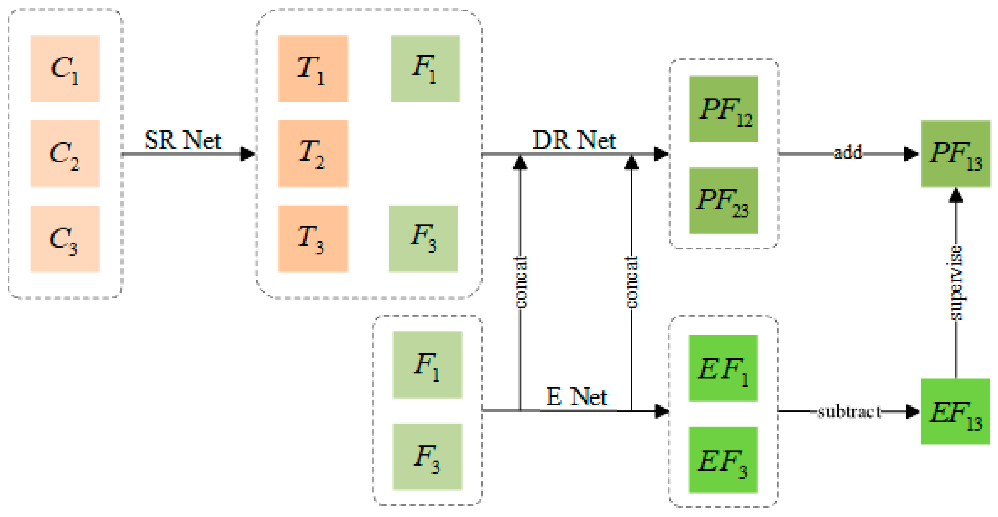
The training process for our model is shown in Figure 1. First, the coarse images from different times are converted into a transitional image matching the fine images through the super-resolution network (SR Net) and then the transitional images at different times are processed into transitional difference images. The second step is to input the corresponding data based on the previous time and based on the next time into the same difference reconstruction network (DR Net) and high-frequency feature extraction network (E Net), respectively, for parameter sharing training. The fine-difference image is predicted according to the structural correlation between the coarse and fine images. The DR Net establishes a nonlinear relationship between the transitional difference image and the fine difference image and the two pieces of feature extraction information from E Net are fused in the reconstruction process of the fine difference image. The and images generated by E Net are processed based on difference, so that the fine difference images reconstructed by DR Net are subject to a feature-level time-series constraint. Through this model, the fine-difference image based on the previous time and the fine-difference image based on the later time are reconstructed as the prior information of the fine image at the fusion time . Each module is described in detail in Section 2.2, Section 2.3 and Section 2.4.
2.2. Super-Resolution Network
The mapping relationship between the earliest coarse images and thin images is simply handled as a super-resolution operation, but spatiotemporal fusion is not exactly a super-resolution problem. One difference is that the magnification of the coarse image is generally 16 for spatiotemporal fusion and the large magnification factor causes the simple super-resolution network to suffer a severe loss of the texture details in the coarse image, thus, failing to meet the needs of spatiotemporal fusion for remote sensing images. Second, because of the richness of remote sensing data sources, there will always be small deviations in data collected at different times, so simple super-resolution structures cannot directly affect spatiotemporal fusion. In StfNet, a method more suitable for remote sensing spatiotemporal fusion is proposed, which combines the coarse difference image and the fine image into the input model, so as to use the spatial information of adjacent fine images and use the time dependence to predict two unknown fine difference images [25]. However, the difference processing is performed at the raw pixel level, resulting in very limited coarse image information that the network can obtain.
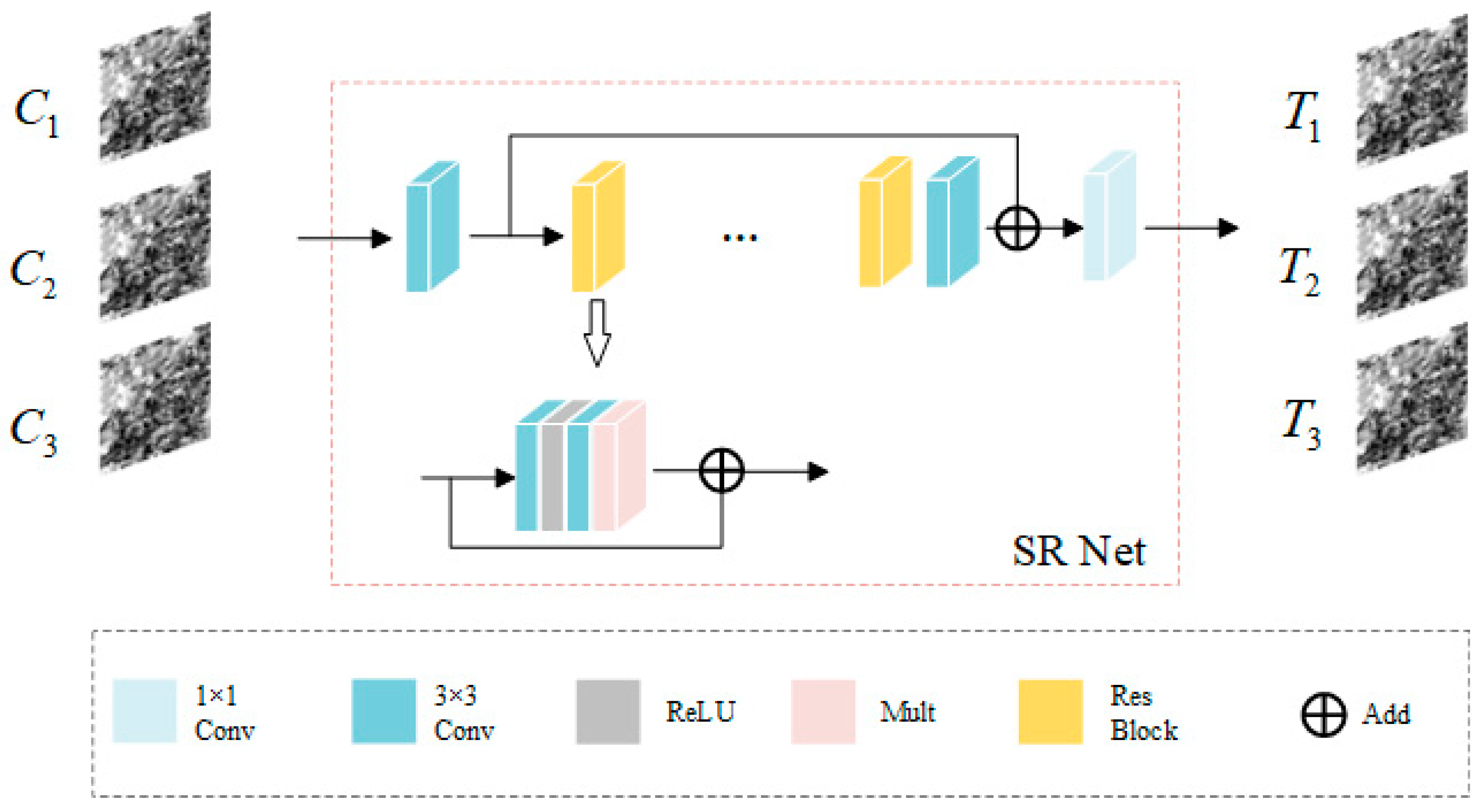
Our proposed model first uses the SR Net to enhance the coarse image to obtain a transitional image that matches the fine image, as shown in Figure 2. A simple mapping relationship between coarse images and fine images is established through the SR Net. The input of the network is , the output is a transition image, which is represented as , and the coarse images at three times are, respectively, input into SR Net for pixel enhancement. The structure of SR Net is inspired by the EDSR network [35]. As the super-resolution reconstruction network is a low-level vision task, the residual block (Res Block) structure in EDSR is chosen to achieve pixel enhancement and preserve spatial information to a higher extent. The residual structure removes the batch normalization layer, which simplifies the previous residual structure and achieves better performance in the super-resolution task. The SR Net is composed of multiple Res blocks, each Res block is composed of two convolutions (one activation and one scaling layer), and a constant scaling layer is placed after the last convolutional layer to stabilize the training process. The number of channels in each residual block is set to 32, so the network needs to first go through a 3 × 3 convolutional network to convert the number of channels to 32 and the network finally restores the output image through a 1 × 1 convolution. The number of Res blocks is discussed later. We express this process using Equation (1).
where represents the SR Net process, represents the coarse image at time , and represents the transition image at time output by the SR network. Here, .
2.3. Difference Reconstruction and High-Frequency Feature Extraction Network
Given that remote sensing images are susceptible to external influences, such as cloud layer, weather, and terrain changes, the information collected at different times is different. Therefore, directly establishing the mapping relationship between transitional and fine images is not suitable for remote sensing tasks. The difference reconstruction network (DR Net) uses the time change information in the image to complete the reconstruction and uses the fine-image information of adjacent moments as a supplement to the spatial detail information. DR Net uses structural similarity in the time series of remote sensing images to finally reconstruct the fine difference image. We define difference images for coarse sequence images, transitional sequence images, and fine sequence images as follows:
where represent the coarse, transitional, and fine images, respectively, while and represent the moments in the time series. represents the change area of the transitional image from to time period, which is also called the transitional difference image from time to time . Here, .
The nonlinear mapping relationship between and is directly established in StfNet, without considering the high-frequency information in the coarse image, and the images generated by different satellite sensors are essentially different. Direct fusion at the original pixel level will lead to the loss of high-frequency information in the fusion result and the blurring of texture details. The model also uses the two-stream network model to map forward and backward dates, resulting in a large amount of network computing. Therefore, our model uses the SR Net to upgrade the coarse image to a transitional image that matches the fine image, enhances its high-frequency information, and then sends it to the DR Net to establish a nonlinear mapping of the fine differential image. DR Net uses temporal correlation for reconstruction and the reconstructed picture is used as a priori information for predicting fine images. As we do not establish the mapping relationship at the original pixel level, we do not use the two-stream network to establish the mapping relationship between different dates. Instead, we use the shared network to train the subdivision images of the forward and backward dates, reduce network computation, and learn more hidden associations. The high-frequency feature extraction network (E Net) inputs the extracted features into the difference reconstruction network for high-frequency feature supplementation. The present spatiotemporal fusion models are all just stitching input networks using adjacent fine images at the beginning, but because remote sensing images have very rich texture details and complex heterogeneous regions, the degree of acquisition of high-frequency features is not enough, which will lead to blurring, distortion, and loss of edge information in the final result map. Therefore, it is necessary to use a separate high-frequency feature extraction network for feature extraction of fine images. E Net extracts high-frequency spatial features of fine images at different moments through multi-scale extraction and convolutional kernel adaptive mechanism, before connecting the extracted features into DR Net to assist DR Net to achieve more accurate fine-difference image reconstruction.
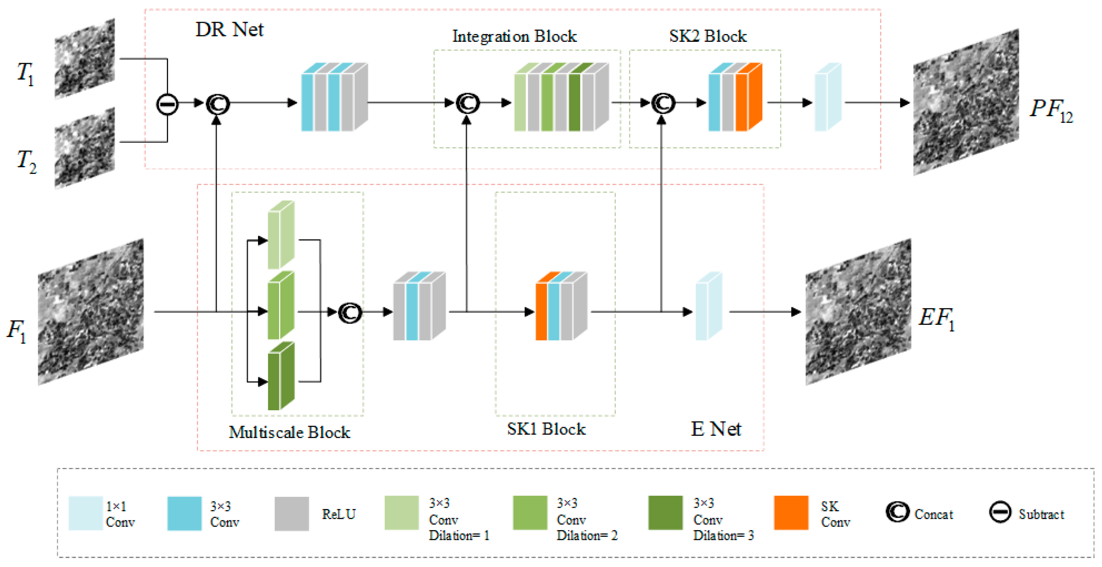
We use time as a reference image to explain the training process for the network. As shown in Figure 3, the fine image at time and the transitional difference images at time and are concatenated as the input of the difference reconstruction network and the fine image at time is used alone as the input of the high-frequency feature extraction network.
E Net consists of a multiscale extraction block (Multiscale Block) and a convolutional kernel adaptive block (SK1 Block) to extract the high-frequency features of . As remote sensing images include very rich feature information, the limited information extracted by using a single type of convolutional layer will lead to poor final fusion results, so we design a multiscale feature extraction module that can reduce training parameters and perceive spatially detailed features at multiple scales more flexibly. This module uses three convolutional layers with different receptive fields to extract feature maps of different scales. In order to avoid problems, such as overfitting, caused by the deeper layers of the network, the block extracts features at different scales in parallel and inputs the extracted features into the subsequent network through concatenation operation. Given that increasing the receptive field will introduce more training parameters, resulting in increased training time, three 3 × 3 dilated convolutions are used to overcome this challenge, with dilation rates of 1, 2, and 3, respectively. Dilated convolution is a filling operation of convolution, which realizes the expansion of the receptive field. The three dilation rates used in the model make the size of the convolution kernel of its convolution layer calculated as 3, 5, and 7. The number of channel mappings for the three convolutional layers is 20 and the three obtained feature maps at different scales are concatenated into a feature map with 60 channels. After 3 × 3 convolution, 64 channel feature maps are adapted for subsequent input into the convolution kernel adaptation block. Furthermore, the high-frequency features extracted by this multi-scale block are fed into the training process of DR Net for feature supplementation. Owing to the large change in remote sensing images in time, the images at different times will have large differences because of external influences and different input images extract different features. Therefore, adding the convolutional kernel adaptive block using a dynamic selection mechanism can adaptively adjust its receptive field size according to multiple scales of the input information, thus, making the whole model more robust and effectively using the spatial information extracted at different scales, so that the model has good performance upon diverse datasets. The convolutional kernel adaptive block is mainly composed using the main structure selection kernel convolution in the selection kernel network [36], which is explained in detail in the next subsection. Similarly, the high-frequency features extracted by the convolutional kernel adaptive block are input into the DR Net training process to assist in the training. E Net finally outputs the image by 1 × 1 convolution, which will be used to constrain the output of the DR Net. The process of E Net can be represented as in Equation (5).
where denotes the high-frequency feature extraction network, denotes the fine image at the time, and denotes the feature image at the time output through E Net. Here, .
DR Net is mainly composed of a feature integration block (Integration Block) and a convolutional kernel adaptation block (SK2 Block). The transitional difference image is concatenated with the fine image as input, the spatial resolution of the fine image is used to provide preliminary texture information, and the difference image is used to locate the temporal changes between the target date and the adjacent dates. The feature integration block is used to integrate the E Net multiscale extraction block to obtain high-frequency features of , which consists of three linearly connected dilated convolutions. For effective use of contextual information in image reconstruction tasks to improve noise removal in the reconstructed images, artifact removal is important [37]. The expansion of the receptive field in convolutional networks is effective for integrating the use of contextual information, but merely increasing the size of the convolutional kernel introduces too many parameters and leads to an increase in training time, so dilated convolution is used. In the feature integration block, 3 × 3 dilated convolution is used, different dilation rates are used to obtain different receptive fields, and the dilation rates are set to 1, 2, and 3. The feature integration module is followed by the convolutional kernel adaptation block (SK2 Block), which reconstructs the high-frequency features extracted by the SK1 Block in E Net and the difference information in this network by integrating them dynamically once again. This block also relies on a selective kernel convolution composition that dynamically adjusts the convolutional kernel weights for different data to suit different predicted images. Finally, the fine-difference image based on the forward time is reconstructed through 1 × 1 convolution. Equation (6) represents its process and Equation (7) is based on the fine-difference image reconstructed at the latter time .
where denotes the difference reconstruction network (DR Net), is the transitional difference image from time to time , is the transitional difference image from time to time , is the fine image at time , is the Multiscale Block in the E Net, and is the SK1 Block in the E Net.
2.4. Select Kernel Convolution
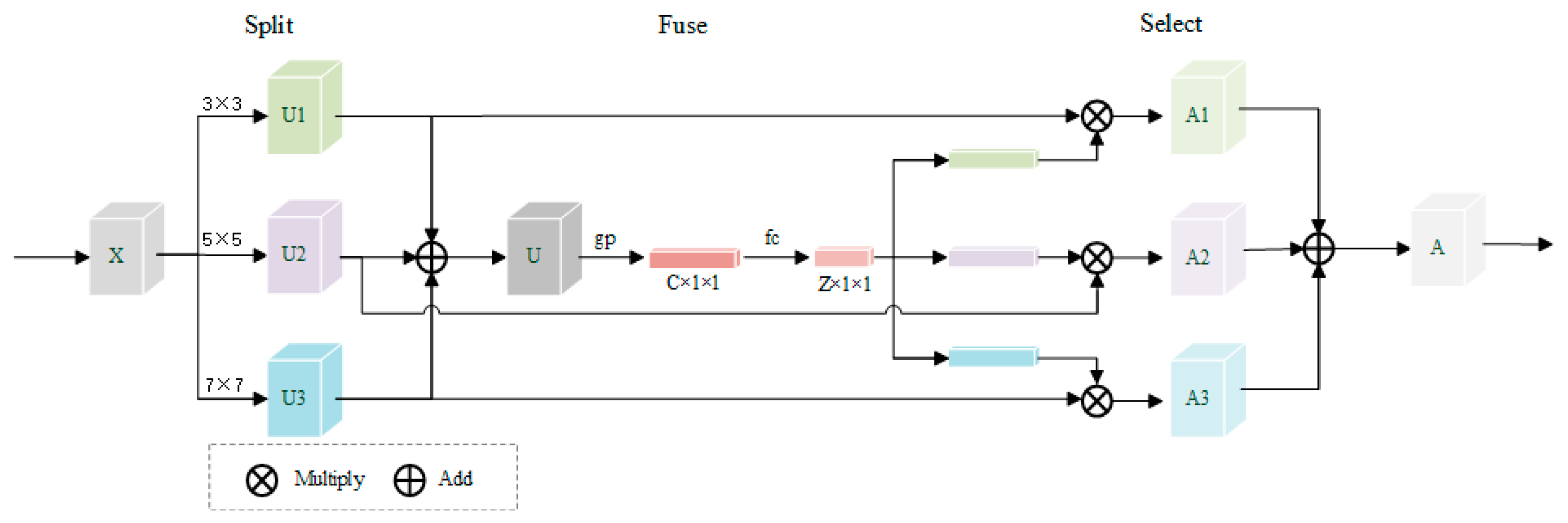
Remote sensing images are inherently complex and variable, so a single receptive field cannot obtain important information from images at multiple scales. The kernel selection mechanism can adjust the receptive field adaptively according to different input information and then dynamically generate convolution kernels. The selective kernel convolution structure used in this study is shown in Figure 4. The purpose of the SK block is to adaptively adjust the receptive field of the network to effectively solve the complex feature extraction problem and the reconstruction problem of different predicted images. Selective kernel is a lightweight embedded block that adaptively adjusts the size of the receptive field as per the multiple scales of the input information. Therefore, the SK block is used in two important network structures, the difference reconstruction network and the high-frequency feature extraction network. Selective kernel convolution is achieved by three operations: split, fuse, and select [36]. In this study, a three-branch structure is used. To improve the efficiency of all three branches, 3 × 3 dilation convolutions are used to collect remote sensing feature information at multiple scales and the dilation rates are set to 1, 2, and 3, which are used to replace the 3 × 3, 5 × 5, and 7 × 7 convolution kernels. The input data X are mapped to U1, U2, and U3 by three branches. In generating the integrated feature map U by element summation, U fuses information from multiple receptive fields, using global average pooling (gp) to generate a one-dimensional vector (C × 1 × 1), which represents the importance of information from each channel. After compressing the information to Z × 1 × 1 size by full connection (fc), it is later reduced to the original size C × 1 × 1 by three linear changes, so that the information extraction of the channel dimension is completed. The three values obtained are then normalized by a SoftMax operator and multiplied by U1, U2, and U3 to obtain A1, A2, and A3, respectively, before adding the three modules to obtain the final result A, which also incorporates information from multiple receptive fields. The experiments prove that SK block has a positive impact on spatiotemporal fusion.
2.5. Training and Prediction
The loss function in remote sensing spatiotemporal fusion models usually uses ℓ2 loss, but ℓ2 cannot capture the complex features of the human visual system, so the performance of ℓ2 loss when applied to image reconstruction tasks is mediocre [38]. To improve the texture details and spectral information in the predicted images, we designed a compound loss function to train the model, which consists of feature loss and content loss, as given in Equation (8).
where the feature loss is computed in the feature space rather than the original pixels and is proposed in the SRPGAN super-resolution model to preserve the essential information in the image [39]. ℓ1 is the mean squared loss, which finds the average between the target and predicted values. ℓ2 loss is the mean squared error, which finds the sum of squares of the differences between the target and predicted values. When the error increases, the ℓ2 loss value increases faster than the ℓ1 loss value. Therefore, the ℓ2 loss is more sensitive to the error outliers. The DR Net output difference image itself has a small value, is prone to error, and is an undetermined image, so the probability of anomaly is higher and we use ℓ1 loss to make the network more robust. The SR Net uses ℓ2 loss, which is more sensitive to outliers and needs to incorporate observations with large errors into the model, which is conducive to network training. Therefore, in our model, the output feature map of training SR Net adopts ℓ2 mean square error and the output feature map of training DR Net adopts ℓ1 mean error. Among them, the DR Net constrained data come from the E Net network, because the high-dimensional feature maps obtained by E Net for feature extraction can constrain their output feature maps more strongly. We define the feature loss of the overall network considering the time correlation constraint and the above reasons as follows.
where is an empirically determined weight parameter to balance the overall network, which we set to 0.2, and is the number of samples. is the transitional difference image from to time and is the fine-difference image from time to . Equations (3) and (4) present this. is the sum of the predicted fine-difference image at time and the predicted fine-difference image at time and is the difference image of and into the output of the E Net using the following equation.
Content loss is used to ensure the overall quality of the reconstructed image with regard to color tone and high-frequency information. We use an integrated loss function mixing ℓ1 and , because may be more sluggish to luminance and color changes, but can retain high-frequency information better, whereas ℓ1 can maintain color brightness features better [38]. is a multi-scale , while the measurement system of consists of three modules: luminance , contrast , and structure , defined as follows [40].
Here, and are the final predicted fine image and the real fine image at time , respectively. and denote the mean and standard deviation of image , respectively, denotes the covariance of image and , and are small constants, and is one-half . is composed as in Equation (15).
where , , and are the parameters that define the relative importance of the three components and setting them all to 1 yields , as in Equation (16).
evaluates at multiple scales thereby expanding the observation range of . Given a dyadic pyramid of levels, is defined as
Here, , and the loss function of is as Equation (18).
The overall content loss consists of loss and ℓ1 loss, which preserves spectral information while retaining high-frequency details from the structure, making the reconstructed image more consistent with human visual perception; this is given in Equation (19).
where is a scaling factor to balance the two loss values, which is empirically set to 0.3. Each output and final result of the module is trained using compound loss so that the prediction results of the model are as similar as possible to the real image while retaining spatial and temporal information.
The two fine-difference images and are predicted by the proposed model, combined with the adjacent fine images, respectively, to eliminate the errors existing in the difference images, and then the fine image at time is reconstructed using an adaptive weighting strategy.
where and are the weighted parameters from the predicted image at moments and , respectively.
As similar coarse images may yield more reliable fine-image predictions, we set the weight of the weighting strategy by determining the degree of temporal variation based on the absolute difference between coarse images. When the change between the coarse image at prediction time and the coarse image at time is small, the target image and the predicted result at time are more similar, so the weight parameter formula is defined as follows.
where . is a small constant used to ensure that the denominator is not zero.
3. Experimental Results and Analysis
3.1. Datasets
We evaluate the robustness of our proposed method upon three datasets and compare a range of representative methods in the field to validate the effectiveness of our approach. Each of the three datasets consist of two sets of real Landsat–MODIS surface reflectance image data, with Landsat acquisition images as fine images and MODIS acquisition images as coarse images. Furthermore, the three datasets cover three study sites with diverse spatial and temporal dynamics. The study area for the first dataset was the Coleambally Irrigation Area (CIA), located in southern New South Wales, Australia (34.0034°E, 145.0675°S). The data were collected for 17 pairs of Landsat–MODIS cloud-free image pairs from October 2001 to May 2002, from Lansat-7 ETM+ and MODIS Terra MOD09GA Collection 5, respectively. Given the relatively small size of the irrigated fields in the CAI data, they are considered to be spatially heterogeneous sites.
The second study area was the Lower Gwydir Catchment (LGC), located in northern New South Wales, Australia (149.2815°E, 29.0855°S). The data were collected from 14 Landsat–MODIS available image pairs from April 2004 to April 2005 from Landsat-5 TM and MODIS Terra MOD09GA Collection 5 data. The LGC data consist mainly of large areas of agricultural land and natural vegetation, with high spatial homogeneity, and this time span covers more physical and land-cover changes, with extensive flooding in December 2004, which results in substantial land-cover changes in the images and a more temporally dynamic site [41].
The third research area was the Alu Horqin Banner (AHB), located in the central part of the Inner Mongolia Autonomous Region in Northeastern China (43.3619°N, 119.0375°E). The data were collected for 27 pairs of Landsat–MODIS cloud-free image pairs from May 2013 to December 2018 from Landsat-8 OLI and MODIS Terra MOD09GA Collection 5 data, respectively. The AHB data span a long period of time, focus on many circular pastures and agricultural fields, and feature considerable physical variability owing to crop and other vegetation growth [42].
All Landsat images have six bands, including the blue band (0.45–0.51 µm), the green band (0.53–0.59 µm), the red band (0.64–0.67 µm), the near-infrared band (0.85–0.88 µm), the short-wave infrared-1 band (1.57–1.65 µm), and the short-wave infrared-2 band (2.11–2.29 µm). The MODIS images are geometrically transformed with respect to the corresponding Landsat images. Both Landsat and MODIS images from the AHB dataset were atmospherically corrected by the Quick Atmospheric Correction (QUAC) algorithm [42]. All Landsat images in the LGC and CIA datasets were atmospherically corrected using MODerate resolution atmospheric transmission4 and MODIS images were first upsampled to a spatial resolution of 25 m using the nearest-neighbor algorithm and then aligned with the corresponding Landsat images [41]. We cropped all images to 1200 × 1200 in order to ensure the consistency of the study area. To reduce the input parameters, we scaled the coarse image to 75 × 75. Using three pairs of Landsat–MODIS image pairs at different moments in the same dataset as a set of experimental data, we input each of the three datasets into the model, where 70% of the data are used for training, 15% for validation, and 15% for testing the performance of the model.
3.2. Parameter Setting
The model is implemented in the PyTorch framework and the convolution mostly uses normal 3 × 3 convolution and dilated 3 × 3 convolution, with a 1 × 1 convolution at the end of each module. To optimize the network training, we use Adam-optimized stochastic gradient descent, with an initial learning rate of 1 × 10⁻⁴ and decay weights of 1 × 10⁻⁶. To reduce the operational burden, we input images cut into small patches for experiments. The size of the patch is 15 × 15 and the clipping stride was to 5. All experiments were trained in a Windows 10 Professional environment configured with an Intel Core i9-10920X [email protected] GHz and NVIDIA GeForce RTX 3090 GPU.
3.3. Evaluation
To demonstrate the fusion effect of our model, we compare the experimental results with STARFM [11], FSDAF [19], STFDCNN [24], StfNet [25], and DCSTFN [26] under the same experimental conditions. We choose six quantitative metrics to evaluate the forecast results.
The first metric is the root mean square error (), which measures the deviation between the predicted and actual images and is defined as follows:
Here, and denote the th pixel value in the predicted image and the real image, respectively. is the total number of pixels in the image. The smaller the value, the closer the predicted image is to the real image.
The second metric is structural similarity (), which is used to measure the overall structural similarity between the predicted image and the real image. The definition is given in Equation (16). The range of values is [−1, 1] and the closer the value is to 1, the more similar the predicted image is to the real image.
The third metric is the peak signal ratio () [43], which measures the global size between the predicted image and the real image to predict the quality of the measured image. The definition is as in Equation (23).
where is the maximum possible pixel value in the real image y. A higher value of proves that the quality of the predicted image is better.
The fourth metric is the correlation coefficient (), which is used to indicate the linear correlation between the predicted and real images. It is defined as:
where and are the average values of the predicted image and the real image, respectively. When the value of is closer to 1, the correlation between the predicted image and the real image is better.
The fifth metric is the spectral angle mapper () [44], which is used to measure the spectral distortion in the predicted images. It is defined in Equation (25).
where is the total number of bands. Smaller values indicate better prediction results.
The sixth metric is Erreur Relative Globale Adimensionnelle de Synthèse () [45], used to evaluate the spectral quality of all predicted bands. The definition is as follows.
Here, denotes the ratio of spatial resolution between fine and coarse images. denotes the average value of the real image in the th band. denotes the value in the th band. Smaller values indicate better overall fusion
Overall, the and metrics focus more on spatial details, the metric reflects the distortion of the image, the metric reflects the correlation between the fused image and the actual image, and the and metrics focus on the spectral information in the predicted image.
3.4. Analysis of Results
We fused the three datasets in the same experimental setting using multiple spatiotemporal fusion methods to present the subjective effects and objective metrics of the fusion results for analysis.
3.4.1. Subjective Evaluation
In order to visualize our experimental results, we show the results of the fusion of STARFM, FDASF, STFDCNN, StfNet, DCSTFN, and our proposed model for the three datasets in Figure 5, Figure 6 and Figure 7.
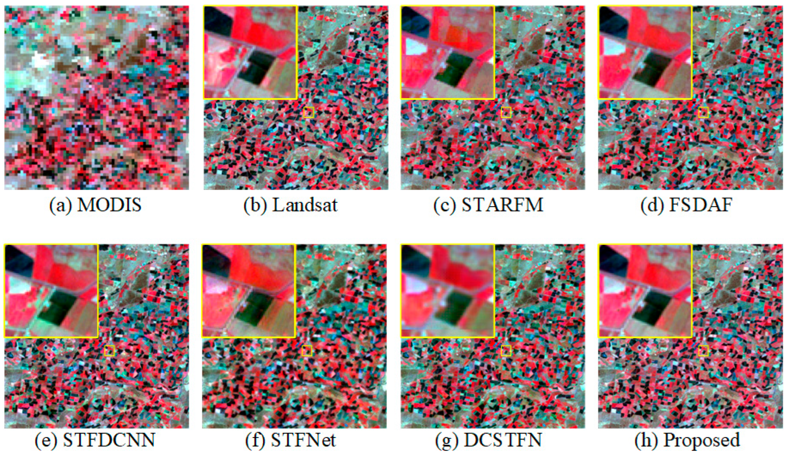
Figure 5 shows the prediction results for the CIA test dataset. Issues, such as blurring, smoothing, and loss of edge information, can be observed in the overall subjective image for StfNet as well as DCSTFN predictions and a lack of spatial detail can be found in the predicted images of both models when locally zoomed in. Square artifacts and a large loss of spectral information in the STARFM predicted images can also be observed in the local detail zoom, while the FDSAF predicted images have insufficient spatial detail and large color differences owing to spectral distortion, while STFDCNN as a whole can be found in multiple places with unidentified green spots and green patches can be clearly observed in the magnified area. Looking at the zoomed-in regions of all models reveals that only the predicted image in our model highly retains the rich spatial detail information and the spectral information in our model is also found to be closer to the real image from the overall image. The subjective presentation of the CIA dataset demonstrates the superiority of our method over other methods.
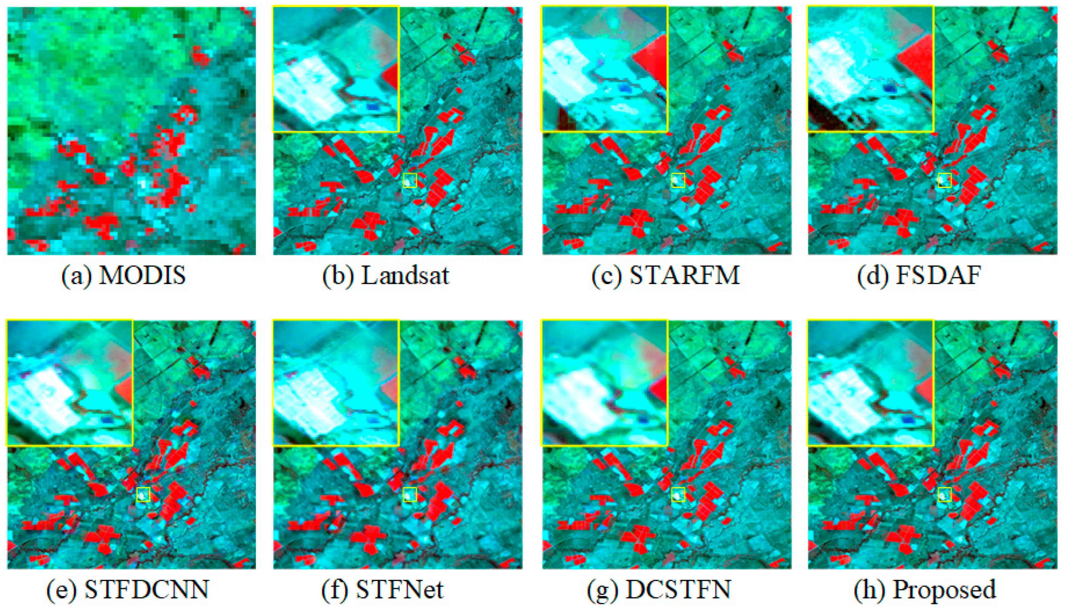
Figure 6 shows the prediction results for each model for the LGC test dataset. Observing the overall predicted image, we see that the predicted image of StfNet is relatively more blurred, while the STFDCNN spectral distortion causes the predicted image to be darker compared to the real image. Observing the enlarged regions of the predicted images of each model, it is found that the FDASF predicted images have severe loss of texture information and loss of image edge information, while the predicted images of STARFM also have relatively blurred spatial details and have image smoothing. In contrast, the predicted images of StfNet and DCSTFN in the deep learning method are zoomed in to observe that their spatial texture information is relatively blurred and DCSTFN is accompanied by a little spectral distortion. The processing of STFDCNN spatial details is better compared to other prediction maps, but its spectral processing is not as good as our model. Overall, the predicted images in our model have better spatial detail and more accurate spectral information compared to other models in the LGC dataset. Therefore, the prediction results of our model are intuitively optimal.
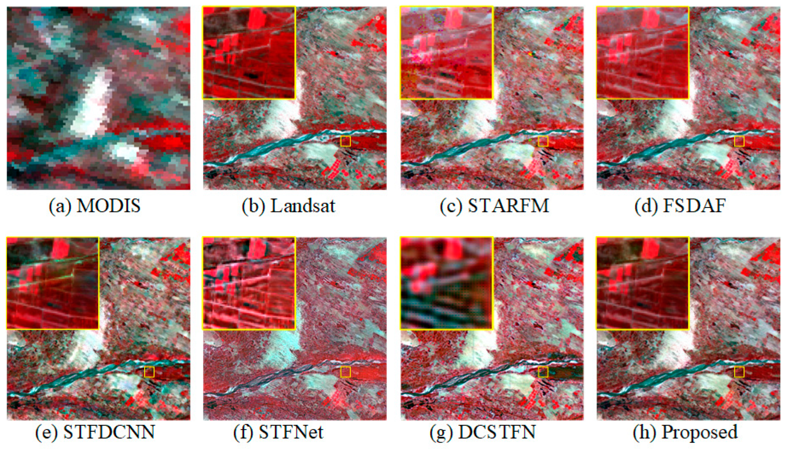
Figure 7 shows a plot of the prediction results for the AHB test dataset on each model. From the overall observation, we can find that the spectral information in the predicted image of StfNet is seriously distorted, the red module of the prediction map is much more than the real image, and the prediction effect is poor in general. The DCSTFN prediction image is also relatively poor; the enlarged image shows that for the red soil, the prediction information is lost, the prediction map is black, and the spatial details are poorly processed. The spectral information in the STFDCNN predicted image is still problematic, causing the entire image to have different tones from the real image, and green spots can be seen to be produced by zooming in on the details. The overall results of STARFM and FDASF are better compared to the other models, but the zoomed-in details show that STARFM predicts incomplete image information with white dot distribution and blurred spatial details, while FSDAF predicts blurred image texture information with unclear edges. The images predicted by our model are, in general, closer to the real images in terms of spectral information and the processing of spatial details is better than other models. The subjective presentation of the prediction results for all three datasets demonstrates that our model outperforms other models; the two-branch structure allows our model to better capture spatial details and the selective kernel block makes our model more robust.
3.4.2. Objective Evaluation
We use six metrics to objectively evaluate the fusion effect of each model. Table 1, Table 2 and Table 3 summarize the objective metric values for the three datasets fused by different models. We show the local metrics RMSE, SSIM, PSNR, and CC for each of the six bands of each dataset and also show the average value of each metric for each of the six bands. The global metrics SAM and ERGAS for the fusion results of the three datasets are also listed in the respective tables. The best value of each metric is in bold. It can be observed that our model achieves the best global metrics in all three datasets, indicating that our model is significantly better than the others for spectra. Band 4 is susceptible to changes in vegetation and bands 5 and 6 are susceptible to changes in surface wetness [41], but experiments on the three different characteristics of the dataset show that the objective indicators for each band are more stable and outperform most models. This also demonstrates the robustness of our model for each band. As can be observed from the statistical CIA dataset in Table 1, our metrics fluctuate in individual bands, but we still reach the optimum in most metrics and the fluctuating indicator values are less different from the optimum. This also proves that our model works better for spatial details on CIA datasets. Table 2 presents the metrics of the LGC dataset and we can see that our model achieves the optimal metrics in each band, which also proves that our model is optimal for LGC data processing. Table 3 presents the indicators of the AHB dataset and it can be observed that very few band indicators of FSDAF reach the optimum on the AHB data, but each indicator in our model reaches the optimum on the average, which indicates the better generalization ability of our model. The objective metrics demonstrated by the three datasets also demonstrate that our model outperforms other comparative models in that our model better captures spatial and spectral information and predicts land-cover changes
4. Discussion
Our model uses MODIS and Landsat data of adjacent moments for predictions. A two-branch structure is used to improve the model’s ability to acquire spatial details, a convolution kernel adaptation block is used to improve the accuracy of various predicted image reconstructions, and a compound loss function is used to improve the training effect. Subjective effects as well as objective metrics on the three datasets demonstrate the superiority of our model. Our model performs better on the CIA dataset with spatially heterogeneous sites, the LGC dataset with rich spatial spectral variability, and the AHB dataset with substantial physical variability. To demonstrate the important contribution of each module in the model, we perform five sets of comparison experiments on a representative LGC dataset using a controlled variation approach in the same experimental setting. The first set of comparison experiments was performed to verify the role of the convolution kernel adaptive block in our model, which we replaced with a simple 3 × 3 convolution. In the second set of comparative experiments, in order to prove the effect of double-branch extraction, we directly removed the high-frequency feature extraction network E Net. In the third set of comparison experiments, we verified the effectiveness of the Multiscale Block in the E Net, so we used 3 × 3 convolution instead. The fourth set of comparison experiments verified the effectiveness of the feature Integration Block in the DR Net, so we used 3 × 3 convolution instead. For the fifth set of comparison experiments, we verified the usefulness of our proposed composite loss function for the model and we used the commonly used ℓ2 loss for the experiments.
Table 4 provides statistics on the objective indicators for the above comparison experiments. The first row of “No-SK” has much lower metrics, indicating that the convolution kernel adaptive block has a larger role in our model, characterized by its processing of spectral information. The second row of “No-ER” is also relatively poor, which also indicates the effectiveness of the high-frequency feature extraction network for the model. The penultimate row, “L2-loss”, shows the metrics after replacing the compound loss in our model with ℓ2 loss, which demonstrates the training effect of compound loss on spatial and spectral information acquisition. There is also the influence of the small blocks in the model on the prediction results and the indicators of “No-MB” and “No-IB” also have some influence on the model. Overall, the design of each module in our model is valid.
In order to investigate the specific design of the super-resolution network, SR Net, in the model, we compared different Res Block depths in the same experimental setting to explore the design of its module depth. For datasets with different characteristics, the depth of the super-resolution network has different effects on the extraction of coarse images and, therefore, has an impact on the final prediction results. In order to achieve better prediction results, we analyze the objective metrics of the prediction results of super-resolution networks having various depths.
Table 5 presents the objective indicators of the prediction results for each dataset when the Res Block depth is 4, 8, and 16, respectively. The CIA dataset contains a large number of small soil areas, making the spatial details more complex, so better results can be achieved by using a deeper SR network. The LGC dataset mainly contains land-cover changes with simpler spatial details, so the best results can be obtained by using an eight-layer SR network. AHB has a large number of small circular pastures and farmlands with complex spatial details, so using 16 layers of SR can achieve better results. However, on balance, the eight-layer- as well as the 16-layer-depth SR Net predicted better than the other models and the effect of our SR depth on the effectiveness of our model was smaller. However, as the training time will increase with deeper depth, we recommend a model with a depth of 8 for other datasets.
Although our model performs well on all three datasets, it has certain shortcomings. As remote sensing data are subject to atmospheric pollution with fewer images that can be used and our model needs to use data from three pairs of coarse and fine images for training prediction, the lack of datasets leads to an insufficient model training effect. Later, better prediction results are considered based on a reduction in model inputs or more flexible selection of input data. In addition, as most models now use single-band image input leading to spectral distortion in the final result, a subsequent improvement in the fusion method investigates how to balance the spectral information in each band while ensuring spatial resolution.
5. Conclusions
The remote sensing spatiotemporal fusion proposed in this paper is based on a convolutional neural network using a two-branch structure and a convolutional kernel adaptive mechanism. A new network structure and compound loss function are used to improve the accuracy of the fusion results. The advantages of our model are as follows:
1. A two-branch structure is adopted, using different networks for information extraction for different tasks, making the overall network structure more flexible and more suitable for remote sensing spatiotemporal fusion tasks. One branch is used to extract the high-frequency features of the fine image, which is then concatenated on the reconstruction network to provide the required high-frequency features for the reconstruction of the image. This branch uses a multiscale extraction block and a convolutional kernel adaptive extraction block to achieve the extraction of multiscale feature information and the experiments also prove the effectiveness of this block. The other branch implements the differential reconstruction task, dilated convolution is used to form a feature integration module, which improves the computational efficiency of the model and effectively organizes various feature information to prevent the loss of spatial information and spectral information.
2. The convolutional kernel adaptive mechanism is used in both branch networks to dynamically adjust the convolutional kernel size for various inputs and to perform adaptive processing for the rich information content of remote sensing images and to better handle the differences in temporal information of remote sensing images, so that the entire network can obtain better performance and increase the adaptive capability of the network.
3. A new compound loss function is used to help network training. The compound loss function consists of feature loss and content loss, which can help reconstruct images to retain similarity in structure, brightness, and spatial details. The super-resolution network is also used to upgrade the coarse image to a transition image that can be matched to the fine image for better performance of subsequent tasks.
Experiments on three disparate datasets with different characteristics also demonstrate that the predicted images in our model have better results in spectral and spatial details and objective metrics demonstrate the superiority and robustness of our model. Future improvements may include flexibility in the handling of the input reference image, reducing the influence of the reference image on the results, as well as exploiting the strengths of traditional algorithms and focusing on the sensitivity of the model to error.
Author Contributions
Data curation, W.L.; formal analysis, W.L.; methodology, W.L. and F.W.; validation, F.W.; visualization, F.W.; writing—original draft, F.W.; writing—review and editing, F.W. and D.C. All authors have read and agreed to the published version of the manuscript.
Funding
This work was supported by the National Natural Science Foundation of China [Nos. 61972060 and 62027827], National Key Research and Development Program of China (No. 2019YFE0110800), and Natural Science Foundation of Chongqing [cstc2020jcyj-zdxmX0025, cstc2019cxcyljrc-td0270].
Data Availability Statement
Data sharing is not applicable to this article.
Acknowledgments
The authors would like to thank all of the reviewers for their valuable contributions to our work.
Conflicts of Interest
The authors declare no conflict of interest.
References
- Zhu, X.; Cai, F.; Tian, J.; Williams, T.K. Spatiotemporal Fusion of Multisource Remote Sensing Data: Literature Survey, Taxonomy, Principles, Applications, and Future Directions. Remote Sens. 2018, 10, 527. [Google Scholar] [CrossRef]
- Kumari, N.; Srivastava, A.; Dumka, U.C. A Long-Term Spatiotemporal Analysis of Vegetation Greenness over the Himalayan Region Using Google Earth Engine. Climate 2021, 9, 109. [Google Scholar] [CrossRef]
- Martín-Ortega, P.; García-Montero, L.G.; Sibelet, N. Temporal Patterns in Illumination Conditions and Its Effect on Vegetation Indices Using Landsat on Google Earth Engine. Remote Sens. 2020, 12, 211. [Google Scholar] [CrossRef]
- Schneider, A. Monitoring land cover change in urban and peri-urban areas using dense time stacks of Landsat satellite data and a data mining approach. Remote Sens. Environ. 2012, 124, 689–704. [Google Scholar] [CrossRef]
- Yu, Q.; Gong, P.; Clinton, N.; Biging, G.; Kelly, M.; Schirokauer, D.J.P.E.; Sensing, R. Object-based detailed vegetation classification with airborne high spatial resolution remote sensing imagery. Photogramm. Eng. Remote Sens. 2006, 72, 799–811. [Google Scholar] [CrossRef]
- Bjorgo, E. Using very high spatial resolution multispectral satellite sensor imagery to monitor refugee camps. Int. J. Remote Sens. 2000, 21, 611–616. [Google Scholar] [CrossRef]
- Johnson, M.D.; Hsieh, W.W.; Cannon, A.J.; Davidson, A.; Bédard, F. Crop yield forecasting on the Canadian Prairies by remotely sensed vegetation indices and machine learning methods. Agric. For. Meteorol. 2016, 218–219, 74–84. [Google Scholar] [CrossRef]
- Zhukov, B.; Oertel, D.; Lanzl, F.; Reinhackel, G.J.I.T.o.G.; Sensing, R. Unmixing-based multisensor multiresolution image fusion. IEEE Trans. Geosci. Remote Sens. 1999, 37, 1212–1226. [Google Scholar] [CrossRef]
- Wu, M.; Niu, Z.; Wang, C.; Wu, C.; Wang, L.J.J.o.A.R.S. Use of MODIS and Landsat time series data to generate high-resolution temporal synthetic Landsat data using a spatial and temporal reflectance fusion model. J. Appl. Remote Sens. 2012, 6, 063507. [Google Scholar] [CrossRef]
- Wu, M.; Huang, W.; Niu, Z.; Wang, C. Generating Daily Synthetic Landsat Imagery by Combining Landsat and MODIS Data. Sensors 2015, 15, 24002–24025. [Google Scholar] [CrossRef] [Green Version]
- Gao, F.; Masek, J.; Schwaller, M.; Hall, F. On the blending of the Landsat and MODIS surface reflectance: Predicting daily Landsat surface reflectance. IEEE Trans. Geosci. Remote Sens. 2006, 44, 2207–2218. [Google Scholar] [CrossRef]
- Zhu, X.; Chen, J.; Gao, F.; Chen, X.; Masek, J.G.J.R.S.o.E. An enhanced spatial and temporal adaptive reflectance fusion model for complex heterogeneous regions. Remote Sens. Environ. 2010, 114, 2610–2623. [Google Scholar] [CrossRef]
- Liu, M.; Liu, X.; Wu, L.; Zou, X.; Jiang, T.; Zhao, B. A Modified Spatiotemporal Fusion Algorithm Using Phenological Information for Predicting Reflectance of Paddy Rice in Southern China. Remote Sens. 2018, 10, 772. [Google Scholar] [CrossRef]
- Cheng, Q.; Liu, H.; Shen, H.; Wu, P.; Zhang, L. A Spatial and Temporal Nonlocal Filter-Based Data Fusion Method. IEEE Trans. Geosci. Remote Sens. 2017, 55, 4476–4488. [Google Scholar] [CrossRef]
- Wang, J.; Huang, B. A Rigorously-Weighted Spatiotemporal Fusion Model with Uncertainty Analysis. Remote Sens. 2017, 9, 990. [Google Scholar] [CrossRef]
- Xue, J.; Leung, Y.; Fung, T. A Bayesian Data Fusion Approach to Spatio-Temporal Fusion of Remotely Sensed Images. Remote Sens. 2017, 9, 1310. [Google Scholar] [CrossRef]
- Xue, J.; Leung, Y.; Fung, T. An Unmixing-Based Bayesian Model for Spatio-Temporal Satellite Image Fusion in Heterogeneous Landscapes. Remote Sens. 2019, 11, 324. [Google Scholar] [CrossRef]
- He, C.; Zhang, Z.; Xiong, D.; Du, J.; Liao, M. Spatio-Temporal Series Remote Sensing Image Prediction Based on Multi-Dictionary Bayesian Fusion. ISPRS Int. J. Geo-Inf. 2017, 6, 374. [Google Scholar] [CrossRef]
- Zhu, X.; Helmer, E.H.; Gao, F.; Liu, D.; Chen, J.; Lefsky, M.A.J.R.S.o.E. A flexible spatiotemporal method for fusing satellite images with different resolutions. Remote Sens. Environ. 2016, 172, 165–177. [Google Scholar] [CrossRef]
- Liu, M.; Yang, W.; Zhu, X.; Chen, J.; Chen, X.; Yang, L.; Helmer, E.H. An Improved Flexible Spatiotemporal DAta Fusion (IFSDAF) method for producing high spatiotemporal resolution normalized difference vegetation index time series. Remote Sens. Environ. 2019, 227, 74–89. [Google Scholar] [CrossRef]
- Gevaert, C.M.; García-Haro, F.J. A comparison of STARFM and an unmixing-based algorithm for Landsat and MODIS data fusion. Remote Sens. Environ. 2015, 156, 34–44. [Google Scholar] [CrossRef]
- Huang, B.; Song, H.J.I.T.o.G.; Sensing, R. Spatiotemporal reflectance fusion via sparse representation. IEEE Trans. Geosci. Remote Sens. 2012, 50, 3707–3716. [Google Scholar] [CrossRef]
- Liu, X.; Deng, C.; Wang, S.; Huang, G.-B.; Zhao, B.; Lauren, P.J.I.G.; Letters, R.S. Fast and accurate spatiotemporal fusion based upon extreme learning machine. IEEE Geosci. Remote Sens. Lett. 2016, 13, 2039–2043. [Google Scholar] [CrossRef]
- Song, H.; Liu, Q.; Wang, G.; Hang, R.; Huang, B.J.I.J.o.S.T.i.A.E.O.; Sensing, R. Spatiotemporal satellite image fusion using deep convolutional neural networks. IEEE J. Sel. Top. Appl. Earth Obs. Remote Sens. 2018, 11, 821–829. [Google Scholar] [CrossRef]
- Liu, X.; Deng, C.; Chanussot, J.; Hong, D.; Zhao, B.J.I.T.o.G.; Sensing, R. StfNet: A two-stream convolutional neural network for spatiotemporal image fusion. IEEE Trans. Geosci. Remote Sens. 2019, 57, 6552–6564. [Google Scholar] [CrossRef]
- Tan, Z.; Yue, P.; Di, L.; Tang, J.J.R.S. Deriving high spatiotemporal remote sensing images using deep convolutional network. Remote Sens. 2018, 10, 1066. [Google Scholar] [CrossRef]
- Tan, Z.; Di, L.; Zhang, M.; Guo, L.; Gao, M.J.R.S. An enhanced deep convolutional model for spatiotemporal image fusion. Remote Sens. 2019, 11, 2898. [Google Scholar] [CrossRef]
- Yin, Z.; Wu, P.; Foody, G.M.; Wu, Y.; Liu, Z.; Du, Y.; Ling, F.J.I.T.o.G.; Sensing, R. Spatiotemporal fusion of land surface temperature based on a convolutional neural network. IEEE Trans. Geosci. Remote Sens. 2020, 59, 1808–1822. [Google Scholar] [CrossRef]
- Chen, Y.; Shi, K.; Ge, Y.; Zhou, Y. Spatiotemporal Remote Sensing Image Fusion Using Multiscale Two-Stream Convolutional Neural Networks. IEEE Trans. Geosci. Remote Sens. 2021, 60, 9116. [Google Scholar] [CrossRef]
- Jia, D.; Song, C.; Cheng, C.; Shen, S.; Ning, L.; Hui, C. A Novel Deep Learning-Based Spatiotemporal Fusion Method for Combining Satellite Images with Different Resolutions Using a Two-Stream Convolutional Neural Network. Remote Sens. 2020, 12, 698. [Google Scholar] [CrossRef] [Green Version]
- Chen, J.; Wang, L.; Feng, R.; Liu, P.; Han, W.; Chen, X.J.I.T.o.G.; Sensing, R. CycleGAN-STF: Spatiotemporal fusion via CycleGAN-based image generation. IEEE Trans. Geosci. Remote Sens. 2020, 59, 5851–5865. [Google Scholar] [CrossRef]
- Tan, Z.; Gao, M.; Li, X.; Jiang, L. A Flexible Reference-Insensitive Spatiotemporal Fusion Model for Remote Sensing Images Using Conditional Generative Adversarial Network. IEEE Trans. Geosci. Remote Sens. 2022, 60, 5601413. [Google Scholar] [CrossRef]
- Chen, G.; Jiao, P.; Hu, Q.; Xiao, L.; Ye, Z. SwinSTFM: Remote Sensing Spatiotemporal Fusion Using Swin Transformer. IEEE Trans. Geosci. Remote Sens. 2022, 60, 5410618. [Google Scholar] [CrossRef]
- Yang, G.; Qian, Y.; Liu, H.; Tang, B.; Qi, R.; Lu, Y.; Geng, J. MSFusion: Multistage for Remote Sensing Image Spatiotemporal Fusion Based on Texture Transformer and Convolutional Neural Network. IEEE J. Sel. Top. Appl. Earth Obs. Remote Sens. 2022, 15, 4653–4666. [Google Scholar] [CrossRef]
- Lim, B.; Son, S.; Kim, H.; Nah, S.; Mu Lee, K. Enhanced deep residual networks for single image super-resolution. In Proceedings of the IEEE Conference on Computer Vision and Pattern Recognition Workshops, Honolulu, HI, USA, 21–26 July 2017; pp. 136–144. [Google Scholar]
- Li, X.; Wang, W.; Hu, X.; Yang, J. Selective kernel networks. In Proceedings of the IEEE/CVF Conference on Computer Vision and Pattern Recognition, Long Beach, CA, USA, 15–20 June 2019; pp. 510–519. [Google Scholar]
- Yuan, Q.; Zhang, L.; Shen, H. Hyperspectral Image Denoising With a Spatial–Spectral View Fusion Strategy. IEEE Trans. Geosci. Remote Sens. 2014, 52, 2314–2325. [Google Scholar] [CrossRef]
- Zhao, H.; Gallo, O.; Frosio, I.; Kautz, J. Loss Functions for Image Restoration With Neural Networks. IEEE Trans. Comput. Imaging 2017, 3, 47–57. [Google Scholar] [CrossRef]
- Wu, B.; Duan, H.; Liu, Z.; Sun, G. SRPGAN: Perceptual generative adversarial network for single image super resolution. arXiv 2017, arXiv:1712.05927. [Google Scholar] [CrossRef]
- Wang, Z.; Simoncelli, E.P.; Bovik, A.C. Multiscale structural similarity for image quality assessment. In Proceedings of the Thrity-Seventh Asilomar Conference on Signals, Systems & Computers, 2003, Pacific Grove, CA, USA, 9–12 November 2003; pp. 1398–1402. [Google Scholar]
- Emelyanova, I.V.; McVicar, T.R.; Van Niel, T.G.; Li, L.T.; Van Dijk, A.I.J.R.S.o.E. Assessing the accuracy of blending Landsat–MODIS surface reflectances in two landscapes with contrasting spatial and temporal dynamics: A framework for algorithm selection. Remote Sens. Environ. 2013, 133, 193–209. [Google Scholar] [CrossRef]
- Li, J.; Li, Y.; He, L.; Chen, J.; Plaza, A. Spatio-temporal fusion for remote sensing data: An overview and new benchmark. Sci. China Inf. Sci. 2020, 63, 140301. [Google Scholar] [CrossRef] [Green Version]
- Ponomarenko, N.; Ieremeiev, O.; Lukin, V.; Egiazarian, K.; Carli, M. Modified image visual quality metrics for contrast change and mean shift accounting. In Proceedings of the 2011 11th International Conference the Experience of Designing and Application of CAD Systems in Microelectronics (CADSM), Polyana, Ukraine, 23–25 February 2011; pp. 305–311. [Google Scholar]
- Yuhas, R.H.; Goetz, A.F.; Boardman, J.W. Discrimination among semi-arid landscape endmembers using the spectral angle mapper (SAM) algorithm. In Proceedings of the Summaries 3rd Annual JPL Airborne Geoscience Workshop, Pasadena, CA, USA, 1–5 June 1992; pp. 147–149. [Google Scholar]
- Wald, L. Quality of high resolution synthesised images: Is there a simple criterion? In Proceedings of the Third Conference “Fusion of Earth Data: Merging Point Measurements, Raster Maps and Remotely Sensed Images”, Sophia Antipolis, France, 26–28 January 2000; pp. 99–103. [Google Scholar]
Figure 1.
Model training flowchart. Here, the SR Net, the DR Net, and the E Net, , , and represent coarse, fine, and transitional images acquired at time and represents fine difference images between and .
Figure 1.
Model training flowchart. Here, the SR Net, the DR Net, and the E Net, , , and represent coarse, fine, and transitional images acquired at time and represents fine difference images between and .

Figure 2.
SR Net architecture. The coarse images () at three times are, respectively, input into SR Net for pixel enhancement and the transition images () are output.
Figure 2.
SR Net architecture. The coarse images () at three times are, respectively, input into SR Net for pixel enhancement and the transition images () are output.

Figure 3.
DR Net and E Net Architecture of the training process at time . The E Net uses the Multiscale Block and SK1 Block to extract the high-frequency information of fine image and then concatenate it into DR Net to assist DR Net to achieve more accurate fine-difference image reconstruction. DR Net is mainly composed of the Integration Block and SK2 Block.

Figure 4.
Selective kernel convolution. Adopt three-branch structure. The convolution kernel size of each branch is 3 × 3, 5 × 5, and 7 × 7, respectively.
Figure 4.
Selective kernel convolution. Adopt three-branch structure. The convolution kernel size of each branch is 3 × 3, 5 × 5, and 7 × 7, respectively.

Figure 5.
Prediction results of Landsat satellite images (8 November 2001) in the CIA dataset. (a) is the corresponding MODIS image, (b) is the real image, (c–g) are the prediction results of STARFM, FSDAF, STFDCNN, StfNet, and DCSTFN models, respectively, and (h) is the prediction result of our model.

Figure 6.
Prediction results of Landsat satellite images (2 March 2005) in LGC dataset. (a) is the corresponding MODIS image, (b) is the real image, (c–g) are the prediction results of STARFM, FSDAF, STFDCNN, StfNet, and DCSTFN models, respectively, and (h) is the prediction result of our model.
Figure 6.
Prediction results of Landsat satellite images (2 March 2005) in LGC dataset. (a) is the corresponding MODIS image, (b) is the real image, (c–g) are the prediction results of STARFM, FSDAF, STFDCNN, StfNet, and DCSTFN models, respectively, and (h) is the prediction result of our model.

Figure 7.
Prediction results of Landsat satellite images (7 July 2015) in the AHB dataset, where (a) is the corresponding MODIS image, (b) is the real image, (c–g) are the prediction results of STARFM, FSDAF, STFDCNN, StfNet, and DCSTFN models, respectively, and (h) is the prediction result of our model.


Table 1.
Objective metrics of different fusion methods for the CIA dataset.
| Evaluation | Band | Method | |||||
|---|---|---|---|---|---|---|---|
| STARFM | FSDAF | STFDCNN | StfNet | DCSTFN | Proposed | ||
| SAM | All | 0.17773 | 0.17796 | 0.16970 | 0.20599 | 0.17169 | 0.15714 |
| ERGAS | All | 2.76449 | 2.78928 | 2.71419 | 2.92699 | 2.72558 | 2.58776 |
| RMSE | Band1 | 0.01060 | 0.01099 | 0.00922 | 0.01250 | 0.01167 | 0.00756 |
| Band2 | 0.01169 | 0.01147 | 0.01013 | 0.01400 | 0.01169 | 0.01015 | |
| Band3 | 0.01708 | 0.01717 | 0.01605 | 0.02100 | 0.01661 | 0.01479 | |
| Band4 | 0.03415 | 0.03361 | 0.03486 | 0.04702 | 0.03078 | 0.03044 | |
| Band5 | 0.04454 | 0.04446 | 0.04414 | 0.04825 | 0.04343 | 0.04014 | |
| Band6 | 0.03639 | 0.03701 | 0.03680 | 0.04147 | 0.03398 | 0.03254 | |
| Average | 0.02574 | 0.02578 | 0.02520 | 0.03071 | 0.02469 | 0.02260 | |
| SSIM | Band1 | 0.94446 | 0.94522 | 0.95646 | 0.92610 | 0.94065 | 0.96267 |
| Band2 | 0.94504 | 0.94562 | 0.95411 | 0.93449 | 0.95058 | 0.95276 | |
| Band3 | 0.90046 | 0.90324 | 0.91601 | 0.88019 | 0.91294 | 0.92034 | |
| Band4 | 0.83292 | 0.84501 | 0.84645 | 0.79357 | 0.86850 | 0.85352 | |
| Band5 | 0.75389 | 0.76793 | 0.79580 | 0.73001 | 0.78953 | 0.77570 | |
| Band6 | 0.76974 | 0.77987 | 0.80288 | 0.72146 | 0.81009 | 0.79169 | |
| Average | 0.85775 | 0.86448 | 0.87862 | 0.83097 | 0.87872 | 0.87611 | |
| PSNR | Band1 | 39.49289 | 39.18375 | 40.70839 | 38.05897 | 38.65891 | 42.42943 |
| Band2 | 38.64465 | 38.80677 | 39.88719 | 37.07460 | 38.64650 | 39.87324 | |
| Band3 | 35.35086 | 35.30671 | 35.88878 | 33.55746 | 35.59164 | 36.60185 | |
| Band4 | 29.33261 | 29.46934 | 29.15324 | 26.55465 | 30.23396 | 30.33128 | |
| Band5 | 27.02466 | 27.04079 | 27.10341 | 26.33000 | 27.24463 | 27.92780 | |
| Band6 | 28.78060 | 28.63450 | 28.68286 | 27.64585 | 29.37578 | 29.75288 | |
| Average | 33.10438 | 33.07364 | 33.57064 | 31.53692 | 33.29190 | 34.48608 | |
| CC | Band1 | 0.84797 | 0.85166 | 0.87150 | 0.83892 | 0.84408 | 0.88373 |
| Band2 | 0.86051 | 0.86298 | 0.88375 | 0.85984 | 0.85926 | 0.88500 | |
| Band3 | 0.87724 | 0.88376 | 0.89932 | 0.88710 | 0.88883 | 0.91565 | |
| Band4 | 0.90270 | 0.91596 | 0.89701 | 0.89356 | 0.92388 | 0.92215 | |
| Band5 | 0.90852 | 0.90987 | 0.91291 | 0.92691 | 0.91272 | 0.92950 | |
| Band6 | 0.90019 | 0.90056 | 0.90333 | 0.91261 | 0.91375 | 0.92361 | |
| Average | 0.88285 | 0.88747 | 0.89464 | 0.88649 | 0.89042 | 0.90994 | |
Table 2.
Objective metrics of different fusion methods for LGC dataset.
| Evaluation | Band | Method | |||||
|---|---|---|---|---|---|---|---|
| STARFM | FSDAF | STFDCNN | StfNet | DCSTFN | Proposed | ||
| SAM | All | 0.21608 | 0.22644 | 0.07604 | 0.09966 | 0.07663 | 0.06262 |
| ERGAS | All | 3.06300 | 3.11580 | 1.81731 | 2.15066 | 1.92113 | 1.65701 |
| RMSE | Band1 | 0.01816 | 0.01835 | 0.00756 | 0.00948 | 0.00810 | 0.00621 |
| Band2 | 0.02400 | 0.02482 | 0.00884 | 0.01168 | 0.00934 | 0.00751 | |
| Band3 | 0.03240 | 0.03393 | 0.01271 | 0.01924 | 0.01334 | 0.01044 | |
| Band4 | 0.05954 | 0.06296 | 0.02088 | 0.02632 | 0.02251 | 0.01647 | |
| Band5 | 0.05706 | 0.06015 | 0.01794 | 0.02791 | 0.02329 | 0.01597 | |
| Band6 | 0.05292 | 0.05618 | 0.01836 | 0.02436 | 0.01785 | 0.01435 | |
| Average | 0.04068 | 0.04273 | 0.01438 | 0.01983 | 0.01574 | 0.01182 | |
| SSIM | Band1 | 0.88757 | 0.88306 | 0.98149 | 0.96998 | 0.97727 | 0.98387 |
| Band2 | 0.83975 | 0.83085 | 0.97864 | 0.95998 | 0.97093 | 0.98036 | |
| Band3 | 0.75378 | 0.73770 | 0.96847 | 0.92825 | 0.95294 | 0.97187 | |
| Band4 | 0.70891 | 0.68867 | 0.96167 | 0.93502 | 0.93549 | 0.96624 | |
| Band5 | 0.56660 | 0.54751 | 0.95494 | 0.90262 | 0.91548 | 0.95579 | |
| Band6 | 0.55919 | 0.53974 | 0.95339 | 0.90927 | 0.92969 | 0.95761 | |
| Average | 0.71930 | 0.70459 | 0.96643 | 0.93419 | 0.94697 | 0.96929 | |
| PSNR | Band1 | 34.81672 | 34.72829 | 42.43257 | 40.46277 | 41.83117 | 44.13334 |
| Band2 | 32.39649 | 32.10473 | 41.06673 | 38.65453 | 40.59295 | 42.49178 | |
| Band3 | 29.78853 | 29.38800 | 37.91901 | 34.31618 | 37.49373 | 39.62743 | |
| Band4 | 24.50316 | 24.01911 | 33.60717 | 31.59294 | 32.95422 | 35.66724 | |
| Band5 | 24.87328 | 24.41488 | 34.92580 | 31.08614 | 32.65612 | 35.93563 | |
| Band6 | 25.52769 | 25.00774 | 34.72062 | 32.26731 | 34.96878 | 36.86193 | |
| Average | 28.65098 | 28.27712 | 37.44532 | 34.72998 | 36.74949 | 39.11956 | |
| CC | Band1 | 0.51162 | 0.50533 | 0.91488 | 0.90620 | 0.92672 | 0.94631 |
| Band2 | 0.45152 | 0.43692 | 0.92854 | 0.91441 | 0.92870 | 0.94757 | |
| Band3 | 0.56210 | 0.53789 | 0.93428 | 0.92169 | 0.93941 | 0.95581 | |
| Band4 | 0.58434 | 0.56634 | 0.95389 | 0.95879 | 0.95941 | 0.97616 | |
| Band5 | 0.69701 | 0.67371 | 0.97069 | 0.96333 | 0.95990 | 0.97726 | |
| Band6 | 0.68504 | 0.65781 | 0.96704 | 0.96466 | 0.96558 | 0.97899 | |
| Average | 0.58194 | 0.56300 | 0.94488 | 0.93818 | 0.94662 | 0.96368 | |
Table 3.
Objective metrics of different fusion methods for the AHB dataset.
| Evaluation | Band | Method | |||||
|---|---|---|---|---|---|---|---|
| STARFM | FSDAF | STFDCNN | StfNet | DCSTFN | Proposed | ||
| SAM | All | 0.17599 | 0.14161 | 0.13987 | 0.20507 | 0.17760 | 0.11674 |
| ERGAS | All | 5.26776 | 5.31239 | 2.97269 | 3.83521 | 3.52752 | 2.52962 |
| RMSE | Band1 | 0.00034 | 0.00034 | 0.00081 | 0.00116 | 0.00155 | 0.00024 |
| Band2 | 0.00577 | 0.00588 | 0.00163 | 0.00275 | 0.00210 | 0.00156 | |
| Band3 | 0.00595 | 0.00610 | 0.00174 | 0.00280 | 0.00234 | 0.00153 | |
| Band4 | 0.00446 | 0.00455 | 0.00144 | 0.00260 | 0.00177 | 0.00139 | |
| Band5 | 0.00145 | 0.00097 | 0.00156 | 0.00239 | 0.00146 | 0.00138 | |
| Band6 | 0.00201 | 0.00105 | 0.00168 | 0.00219 | 0.00149 | 0.00147 | |
| Average | 0.00333 | 0.00315 | 0.00148 | 0.00232 | 0.00178 | 0.00126 | |
| SSIM | Band1 | 0.99931 | 0.99929 | 0.99458 | 0.98874 | 0.97982 | 0.99963 |
| Band2 | 0.86470 | 0.85765 | 0.99037 | 0.97664 | 0.98603 | 0.99057 | |
| Band3 | 0.86977 | 0.86011 | 0.98959 | 0.97450 | 0.98120 | 0.99179 | |
| Band4 | 0.94349 | 0.94068 | 0.99624 | 0.98461 | 0.99390 | 0.99641 | |
| Band5 | 0.99387 | 0.99673 | 0.98949 | 0.97616 | 0.99279 | 0.99235 | |
| Band6 | 0.98878 | 0.99532 | 0.98609 | 0.97613 | 0.99062 | 0.99199 | |
| Average | 0.94332 | 0.94163 | 0.99106 | 0.97946 | 0.98739 | 0.99379 | |
| PSNR | Band1 | 69.42295 | 69.42746 | 61.82981 | 58.67503 | 56.20781 | 72.37595 |
| Band2 | 44.77567 | 44.60654 | 55.73295 | 51.20813 | 53.56492 | 56.15748 | |
| Band3 | 44.51268 | 44.29919 | 55.18479 | 51.06624 | 52.61050 | 56.28335 | |
| Band4 | 47.01360 | 46.83312 | 56.83543 | 51.68850 | 55.03054 | 57.16858 | |
| Band5 | 56.77382 | 60.25078 | 56.12355 | 52.44044 | 56.73506 | 57.22576 | |
| Band6 | 53.94259 | 59.56925 | 55.47859 | 53.20197 | 56.51348 | 56.62752 | |
| Average | 52.74022 | 54.16439 | 56.86419 | 53.04672 | 55.11038 | 59.30644 | |
| CC | Band1 | 0.84204 | 0.86895 | 0.85005 | 0.33176 | 0.00119 | 0.91827 |
| Band2 | 0.86498 | 0.89428 | 0.91020 | 0.86735 | 0.87435 | 0.93430 | |
| Band3 | 0.82886 | 0.90540 | 0.91612 | 0.87905 | 0.86938 | 0.93661 | |
| Band4 | 0.79782 | 0.82082 | 0.78346 | 0.62491 | 0.71780 | 0.84136 | |
| Band5 | 0.79034 | 0.88965 | 0.90013 | 0.15037 | 0.82164 | 0.90385 | |
| Band6 | 0.66197 | 0.89047 | 0.85566 | 0.58300 | 0.81597 | 0.82653 | |
| Average | 0.79767 | 0.87826 | 0.86927 | 0.57274 | 0.68339 | 0.89349 | |
Table 4.
Comparative metrics of the impact of different blocks on the model on the LGC dataset.
| Method | SAM | ERGAS | RMSE | SSIM | PSNR | CC |
|---|---|---|---|---|---|---|
| No-SK | 0.06410 | 1.68862 | 0.01226 | 0.96855 | 38.82388 | 0.96204 |
| No-ER | 0.06376 | 1.66948 | 0.01215 | 0.96908 | 38.92764 | 0.96221 |
| No-MB | 0.06279 | 1.67319 | 0.01224 | 0.96907 | 38.93710 | 0.96365 |
| No-FIB | 0.06379 | 1.66509 | 0.01192 | 0.96895 | 39.02248 | 0.96248 |
| L2-loss | 0.06555 | 1.70390 | 0.01293 | 0.96818 | 38.51485 | 0.96037 |
| Proposed | 0.06262 | 1.65701 | 0.01182 | 0.96929 | 39.11956 | 0.96368 |
Table 5.
Comparative metrics for the impact of super-resolution networks on the model at various depths on the three datasets.
Table 5.
Comparative metrics for the impact of super-resolution networks on the model at various depths on the three datasets.
| Data | Res Block | SAM | ERGAS | RMSE | SSIM | PSNR | CC |
|---|---|---|---|---|---|---|---|
| CIA | 4 | 0.15750 | 2.60573 | 0.02275 | 0.87700 | 34.26018 | 0.90863 |
| 8 | 0.15645 | 2.59462 | 0.02282 | 0.87602 | 34.26894 | 0.90995 | |
| 16 | 0.15714 | 2.58776 | 0.02260 | 0.87611 | 34.48608 | 0.90994 | |
| LGC | 4 | 0.06460 | 1.70334 | 0.01228 | 0.96870 | 38.71426 | 0.96079 |
| 8 | 0.06262 | 1.65701 | 0.01182 | 0.96929 | 39.11956 | 0.96368 | |
| 16 | 0.06247 | 1.71455 | 0.01213 | 0.96877 | 38.76080 | 0.96447 | |
| AHB | 4 | 0.11507 | 2.53645 | 0.00137 | 0.99215 | 58.64425 | 0.90601 |
| 8 | 0.11831 | 2.54526 | 0.00136 | 0.99218 | 59.11255 | 0.89589 | |
| 16 | 0.11674 | 2.52962 | 0.00126 | 0.99379 | 59.30644 | 0.89349 |
Publisher’s Note: MDPI stays neutral with regard to jurisdictional claims in published maps and institutional affiliations. |
© 2022 by the authors. Licensee MDPI, Basel, Switzerland. This article is an open access article distributed under the terms and conditions of the Creative Commons Attribution (CC BY) license (https://creativecommons.org/licenses/by/4.0/).
Share and Cite
MDPI and ACS Style
Li, W.; Wu, F.; Cao, D. Dual-Branch Remote Sensing Spatiotemporal Fusion Network Based on Selection Kernel Mechanism. Remote Sens. 2022, 14, 4282. https://0-doi-org.brum.beds.ac.uk/10.3390/rs14174282
AMA Style
Li W, Wu F, Cao D. Dual-Branch Remote Sensing Spatiotemporal Fusion Network Based on Selection Kernel Mechanism. Remote Sensing. 2022; 14(17):4282. https://0-doi-org.brum.beds.ac.uk/10.3390/rs14174282
Chicago/Turabian StyleLi, Weisheng, Fengyan Wu, and Dongwen Cao. 2022. "Dual-Branch Remote Sensing Spatiotemporal Fusion Network Based on Selection Kernel Mechanism" Remote Sensing 14, no. 17: 4282. https://0-doi-org.brum.beds.ac.uk/10.3390/rs14174282
Note that from the first issue of 2016, this journal uses article numbers instead of page numbers. See further details here.