Full-Coupled Convolutional Transformer for Surface-Based Duct Refractivity Inversion

Abstract

A surface-based duct (SBD) is an abnormal atmospheric structure with a low probability of occurrence buta strong ability to trap electromagnetic waves. However, the existing research is based on the assumption that the range direction of the surface duct is homogeneous, which will lead to low productivity and large errors when applied in a real-marine environment. To alleviate these issues, we propose a framework for the inversion of inhomogeneous SBD M-profile based on a full-coupled convolutional Transformer (FCCT) deep learning network. We first designed a one-dimensional residual dilated causal convolution autoencoder to extract the feature representations from a high-dimension range direction inhomogeneous M-profile. Second, to improve efficiency and precision, we proposed a full-coupled convolutional Transformer (FCCT) that incorporated dilated causal convolutional layers to gain exponentially receptive field growth of the M-profile and help Transformer-like models improve the receptive field of each range direction inhomogeneous SBD M-profile information. We tested our proposed method performance on two sets of simulated sea clutter power data where the inversion of the simulated data reached 96.99% and 97.69%, which outperformed the existing baseline methods.

1. Introduction

As a kind of tropospheric duct, surface-based duct (SBD) can trap electromagnetic waves in the duct layer and seriously interfere with actual maritime radar communications. Thus, high-precision inversion of the modified refractivity profile (M-profile) for SBD can not only provide information about the anomalous spatial distribution of electromagnetic wave propagation but also allow for timely repair measures to correct radar holes generated by the trapping SBD M-profile structure [1]. However, affected by intricate meteorological factors, the distribution of the SBD M-profile in the range direction from the sea surface is inhomogeneous, which presents formidable challenges when modeling the considerable number of parameters of the M-profile and when inverting it through nonlinear relationships with sea clutter. To overcome the inversion challenge caused by the high dimensionality of the M-profile parameters, a principal component analysis (PCA) method was first used to reduce the data dimensionality of the M-profile. However, this standard method is laborious and fails to capture the nonlinear dependency of the SBD M-profile. Therefore, it is urgent that an effective solution for extracting low-dimensional representative features of inhomogeneous SBD M-profiles be developed.

The advent of deep learning caused a revolution in industrial dimensional reduction applications [2]. Typical deep learning models applied for the reduction of high-dimensional spaces incorporate a backpropagation network (BPN), deep belief network (DBN) [3], and stacked auto-encoders (SAE) [4]. However, the above models belong to fully connected networks, and when deployed for feature extraction, excessively high-dimensional data will add too much computational complexity. Paoletti et al. [5] proposed a deep convolutional neural network (CNN) for feature extraction and the classification of images. Han et al. [6] proposed a different-scale two-stream convolutional network for dimensional reduction. However, these networks still require numerous class-label samples for supervised learning. To address this issue, Dasan proposed convolutional denoising autoencoder unsupervised CNN-based methods for electrocardiogram (ECG) signal dimensional reduction [7]. Zhang et al. [8] proposed a CNN network for unsupervised hyperspectral image feature extraction. Nevertheless, these unsupervised CNN-based models still depend on the optimization of many connection weights. To that end, in this study, we employ residual learning and skip the network connection to optimize the CNN structure, and we used dilated causal convolution kernels embedded in auto-encoders for feature learning and dimensional reduction to address this problem.

Although deep learning frameworks based on one-dimensional residual-dilated causal convolution autoencoders (1D-RDCAE) have made remarkable progress in extracting effective and robust features, there remains a lack of a generalized model to construct the relationship between sea clutter and the SBD M-profile. In 2003, Gerstoft et al. employed a genetic algorithm (GA) [9] with a radar clutter reduction technology to inverse the M-profile. Zhang [10] employed a particle swarm optimization (PSO) algorithm to invert a range direction inhomogeneous SBD M-profile. Moreover, a large number of researchers have used machine learning methods in the application of atmospheric ducts and achieved excellent inversion results [11,12,13,14,15,16]. However, both GA, PSO, SVM, and MLP algorithms require repeatedly using parabolic equations of the atmospheric ducts, which is time-consuming. Guo [17] proposed an approach based on deep learning to invert the height of the range-direction homogeneous surface-based ducts in 2019. In 2020, Zhao [18] proposed a method based on a BP neural network to predict the height of the evaporation duct. In 2022, Ji [19] introduced a method based on a Deep Neural Network to predict the height of the evaporation duct. Nevertheless, these models are unable to guarantee the effective inversion of an inhomogeneous SBD M-profile, as using a fully connected layer network that occupies the entire range-direction freedom of the inhomogeneous SBD M-profile will engender overfitting and a large number of calculations during the training network. In addition, inputting the long inhomogeneous sea clutter power sequence into existing deep learning Recurrent Neural Network (RNN), CNN, and fully connected neural networks [17] will lead to overfitting and high computational complexity when inverting a high dimension SBD M-profile.

Recently, Transformer-based models have shown superior performance compared to RNN and CNN-based models in the field of natural language processing. The self-attention mechanism helps model equal availability for any input regardless of temporal distance, allowing Transformer models more potential in dealing with long-sequence information. Lim proposed the Temporal Fusion Transformer to learn temporal relationships at different scales [20]. Zhou proposed the Informer model for forecasting time series [21]. Yin proposed a rainfall-runoff model named RR-Former based on Transformer [22]. However, these deep learning methods are mostly derived from the Vaswani Transformer [23], and they will model quadratically computation cost and memory consumption growth according to the long sequence input [24]. The core of the CNN network is the convolution kernel, which has inductive biases such as translation invariance and can capture local spatiotemporal information. One of the typical applications is the focus mechanism of YoloV5 [25], which can get more fine-grained information, such as the shortcut map in the ResNet model [26], with negligible extra computation costs. Thus, we apply it to the stack of self-attention blocks within the encoder of Transformer. Apart from computer vision tasks, CNN models also hold a foot in time series classification problems, such as TCN [27] and U-Net [28]. The core architecture of these models is to make use of the causal convolutional layer. Instead of applying the whole TCN baseline to Transformer architecture, we only adopt the idea of dilated causal convolution and apply it to connect self-attention blocks to gain exponentially receptive field growth of Transformer.

To this end, our work delves into making full use of the merits of convolutional neural networks and Transformers. Two classic CNN architecture transformations have been successfully applied to the Transformer architecture on the SBD M-profile inversion. The contributions of our work are summarized as follows: (1) We addressed feature extraction from high-dimension M-profiles of inhomogeneous SBD M-profile by proposing an unsupervised learning-based 1D-RDCAE. The experiments indicate that the 1D-RDCAE had dramatically reduced error results, and the model achieved a better fit of the original data compared to the PCA, BPN, SAE, DBN, 1D-CAE, and 1D-RCAE models. Furthermore, 1D-RDCAE provides a solution for extracting low-dimensional representative features of the SBD M-profile. (2) We proposed the idea of full-coupled convolutional Transformer architectures to establish the nonlinear relationship between sea clutter and high-dimensional M-profile parameters. Extensive experiments demonstrate that our proposed architecture not only enhances the Transformer’s learning capability but also cuts down the computational cost and memory usage.

2. Method

2.1. Modeling of the SBD M-Profile

The surface-based duct M-profile is divided into the surface-based duct with a base layer and surface-based duct without a base layer. As shown in Figure 1a, the M-profile with a base layer (three-line refractive index) includes four basic parameters: the height of the base ($z_b$), the thickness of the trapping layer ($z_{\mathrm{thick}}$), the refractive index of the trapping layer ($M_d$), and the slope of the base layer ($c_1$). The M-profile of the three-line refractive index is expressed by the following formula:

$$M\left(z\right)=M_0+\left\{\begin{array}{cc}{c}_{1}z\hfill & z<z_b\hfill \\ c_1{z}_b-M_d\frac{z-z_b}{z_{\mathrm{thick}}}\hfill & z_b<z<z_{\mathrm{thick}}\hfill \\ c_1{z}_b-M_d+0.118\left(z-z_b-z_{\mathrm{thick}}\right)\hfill & z\ge z_{\mathrm{thick}}+z_b\hfill \end{array}\right.,$$

(1)

when $z=0$, that is, the height of the duct is the height of the mean sea level, the corresponding value of M is $M_0=339M-\mathrm{units}$, where $z_b$ and $z_{\mathrm{thick}}$ represent the height of the base layer and the thickness of the trapping layer, respectively. $c_1$ is the slope of the base layer, and $M_d$ is the refractive index of the trapping layer. In our simulations, the parameters are set, as shown in

Table 1. Parameter setting of the three-fold line refractive index M-profile.

Parameter	Lower	Upper
The height of the base (m)	1	100
The thickness of the trapping layer (m)	20	100
The refractive index of the trapping layer (M-units)	20	100
The slope of the base layer	1	20

.

As shown in Figure 1b, the M-profile without a base layer (two-line refractive index) includes two basic parameters: the height of the base ($z_b$), and the refractive index of the trapping layer ($M_d$). The M-profile of the two-line refractive index is expressed by the following formula:

$$M\left(z\right)=M_0+\left\{\begin{array}{cc}kz\hfill & 0<z<z_{\mathrm{thick}}\hfill \\ k{z}_{\mathrm{thick}}+0.118\left(z-z_{\mathrm{thick}}\right)\hfill & z\ge z_{\mathrm{thick}}\hfill \end{array}\right.,$$

(2)

The parameters of the SBD M-profile can be modeled through a Gauss—Markov process [1]. Figure 2 presents the simulation results obtained after using Markov chains with one sample of SBD M-profile parameters for a range of 0–100 km and a range interval of 0.1 km.

2.2. Forward Sea Clutter Power Calculation

The premise of employing radar sea clutter to implement duct inversion is to model the forward propagation of radar electromagnetic waves in the ocean environment. The forward calculation of radar sea clutter power is to reconstruct the parameters of the range direction inhomogeneous M-profile by the low-degree-of-freedom parameters, which is brought into the parabolic equation (PE) and radar sea clutter power calculation formula to calculate the radar sea clutter power. The forward simulation accuracy of radar sea clutter directly determines the inversion quality of the duct. The radar sea clutter is the radar backscatter echo of the rough sea surface [1].

Applying the fundamental principle of radar, we can determine the power of the radar receptance from a target with a distance r and radar cross-section ${\delta }^1$:

$$P_c=\frac{P{}_t{G}_t{\lambda }^2{F}^4{\delta }^1}{{\left(4\pi \right)}^3{r}^{{}^4}}$$

(3)

where $P_t$ and $G_t$ are the transmit power and transmit antenna gain, respectively, $\lambda$ is the wavelength, ${\delta }^1$ is the sea radar cross-section, F is the propagation factor, and r is the distance between the radar and the target. The propagation factor and the loss during propagation have the following relationship:

$$L=\frac{{\left(4\pi r\right)}^2}{{\lambda }^2}\setminus F^2$$

(4)

The sea radar cross-section ${\delta }^1$ can be represented by the scattering coefficient of the sea surface ${\delta }^1$ according to ${\delta }_1=A_c{\delta }^0$, where $A_c$ is the sea illumination area. Therefore, (3) can be represented by (5):

$$P_c=\frac{P{}_t{G}_{t}4\pi A_c{\delta }^0}{L^2{\lambda }^2}$$

(5)

where the illumination area and distance have the following relationship:

$$A_c=\frac{r{\Theta }_{3dB}\tau c}{2cos{\Theta }_g}$$

(6)

Here, ${\Theta }_{3dB}$ is the horizontal radar lobe width, $\frac{\tau c}{2}$ is the resolution of the radar distance, and ${\Theta }_g$ is the grazing angle. When the grazing angle ${\Theta }_g$ has a small value, $cos{\Theta }_g$ is almost a constant. Therefore, the relationship between $A_c$ and r is linear. The power of the radar sea clutter can be represented by (7):

$$P_c=\frac{C_1{\delta }_{0}r}{L^2}$$

(7)

Here, $C_1$ is a constant that depends upon the wavelength of the electromagnetic wave, transmit power, and antenna gain, and it is defined as follows:

$$C_1=\frac{2\pi P_t{G}_t{\Theta }_{3db}\tau c}{{\lambda }^2}$$

(8)

Finally, the power of the radar sea clutter can be represented by the following equation:

$$P_{c,dB}=-2L_{dB}+{\delta }_{dB}^0+10lo{g}_{10}^{\left(r\right)}+C_{dB}$$

(9)

Among them, $L_{dB}$ is the propagation loss and is solved using a parabolic equation model, and ${\delta }_{dB}^0$ is the radar scattering coefficient and is retrieved applying the Georgia Institute of Technology (GIT) empirical model [1].

2.3. SBD M-Profile Dimension Reduction

The high dimensionality of the SBD M-profile results in great computational costs for the forward propagation of sea clutter and the backward inversion process, leading to low efficiency and large errors. To address this issue, we use a 1D-RDCAE to reduce the dimensions of the SBD M-profile parameters.

First, we construct a one-dimension dilated causal convolutional autoencoder network using high-dimensional SBD M-profile parameters as inputs. The optimal mapping of the high-dimensional space into the low-dimensional feature layer is actualized through various dilated causal convolution and pooling layers, thus obtaining a parameter matrix with fewer degrees of freedom. Then, we use a decoder network to perform deconvolution and upsampling so that the outputs coincide with the parameters of the SBD M-profile in the range direction. Third, a residual learning block is embedded in the encoder and decoder networks to resolve feature learning on the range-direction vibration of the SBD M-profile. The root mean square error (RMSE), mean absolute error (MAE), and R-square ($R^2$) are minimized by network training, established as the objective of the 1D-RDCAE, the minimization of the reconstruction error.

The proposed 1D-RDCAE network structure is illustrated in Figure 3. The learning of the 1D-RDCAE network comprises two phases: the encoder and decoder phases. In the encoder stage, dilated causal convolution (that is, Dconv1, Dconv2, …, Dconv4) and pooling layers (that is, Maxpooling1, Maxpooling2, …, Maxpooling4) are applied to encode the SBD M-profile parameters to the low-degree-of-freedom parameter matrix. During the decoding step, de-dilated convolution (that is, Dedeonv1, Dedeonv2, …, Dedeonv4) and upsample layers (that is, Upsample1, Upsample2, …, Upsample4) are used to restore the SBD M-profile. In parallel, the residual block’s (that is, Bottleneck1, and Bottleneck2) learning mechanisms are incorporated into the network to improve its gradient conduction, thus controlling the reconstruction error and enhancing the capacity of the network to extract the features. The detailed steps are as follows.

2.3.1. Encoder Network

The encoder network comprises four one-dimensional dilated causal convolutional layers, four one-dimensional pooling layers, and one bottleneck layer. Figure 4 presents the detailed structure of the encoder and decoder network; for the $i\mathrm{th}$ dilated causal convolutional layer, the dilated causal convolutional operation DConv1d of kernel size h on the $x_n\in R^d$ is defined as

$$\mathrm{DConv}1\mathrm{d}\left(x_n\right)=\left[\begin{array}{c}{x}_n\\ x_{n-i}\\ ⋮\\ x_{n-(h-1)\times i}\end{array}\right]W^{d\times d_{\mathrm{out}}},$$

(10)

where $d_{\mathrm{out}}$ is the output dimension, and i is the dilation factor. When $i=1$, the dilated causal convolution is degraded to canonical causal convolution.

The one-dimensional pooling layers reduce the dimensionality of the input data. For the feature of the $(n+1)$-th layer, the output after pooling is defined as:

$$x_{n+1}=MaxPool\left(\mathrm{RELU}\left(\mathrm{DConv}1d\left(x_n\right)\right)\right)$$

(11)

where DConv1d(.) indicates a 1D dilated causal convolutional filter with the RELU(.) activation function. The bottleneck layer is a specific convolutional layer with a convolution kernel size and stride size of 1. This $1\times 1$ convolution connection performs dimensionality reduction over the channel, and the parameters of the bottleneck layer become feasible. Accordingly, the bottleneck layer can reduce neurons in an FC layer network.

2.3.2. Decoder Network

The decoder network consists of four dilated causal convolution layers, four upsampling layers, and one bottleneck layer, whose function is the inverse of that of the encoder network. From Equation (10), the output of the de-dilated causal convolution layer can be deduced as follows:

$$\mathrm{DeDconv}1\mathrm{d}\left(x_n\right)=\left[\begin{array}{c}{x}_n\\ x_{n-j}\\ ⋮\\ x_{n-(h-1)\times j}\end{array}\right]{\overline{W}}^{d\times d_{\mathrm{out}}},$$

(12)

where ${\overline{W}}^{d\times d_{\mathrm{out}}}$ represents the de-dilated causal convolution kernel. $d_{\mathrm{out}}$ is the output dimension, and j is the dilation factor.

The one-dimensional upsampling layers reduce the dimensionality of the input data. For the feature of the $(n+1)$-th layer, the output after pooling is defined as:

$$x_{n+1}=Upsample(RELU(DeDconv1d\left(x_n\right)))$$

(13)

where DeDconv1d(.) indicates a 1D dilated causal convolutional filter with the RELU(.) activation function. We add an upsampling layer with stride 2 that is then used to downsample x into its half slice after stacking a layer and providing a more focused feature map for the following attention block.

2.3.3. Residual Block

The residual block module transfers data features by jumping connections. For the residual block module in Figure 3, the input of the upsample layer 2 (Upsample2) is:

$$\begin{array}{cc}\hfill X_{u2}& =D^1\left(X{d}_1\right)+p^3\left(X{p}_3\right)\hfill \\ \hfill & =D^1\left(U^1\left(X_{u1}\right)\right)+p^3\left(C^3\left(X\right)\right),\hfill \end{array}$$

(14)

where $D^1$ is de-dilated causal convolution layer 1, $p^3$ is pooling layer 3, $U^1$ is upsample layer 1, $C^3$ is dilated causal convolution layer 3, and X is the input data of pooling layer 3.

The output of upsample 2 is:

$$y_{u2}=U^2\left(X_{u2}\right),$$

(15)

where $U^2$ represents upsample layer 2, and $y_{u2}$ is the output of upsample layer 2.

$$X_{u3}=D^2\left(X_{d2}\right)=D^2\left(y_{u2}\right),$$

(16)

where $D^2$ refers to Deconv 2 layer, $X_{d2}$ is the input to Deconv 2, and $X_{u3}$ is the input data of upsample layer 3.

The reconstruction error is normally determined using the MAE, RMSE, and $R^2$, which are defined as:

$$\begin{array}{cc}\hfill \mathrm{RMSE}& =\sqrt{\frac{{\sum }_{i=1}^n{(g\left(h\left(x\right)\right)-x)}^2}{n}}.\hfill \end{array}$$

(17)

$$\begin{array}{cc}\hfill \mathrm{MAE}& =\frac{1}{n}\sum _{i=1}^n|g\left(h\left(x\right)\right)-x|.\hfill \end{array}$$

(18)

$$\begin{array}{cc}\hfill R^2& =1-\frac{\left({\sum }_{i=1}^n{\left(x-g\left(h\left(x\right)\right)\right)}^2\right)/n}{\left({\sum }_{i=1}^n{\left(\overline{x}-g\left(h\left(x\right)\right)\right)}^2\right)/n},\hfill \end{array}$$

(19)

where x is the initial network status observation matrix input data, $g\left(h\left(x\right)\right)$ is the reconstructed data, which has the same dimensions as the initial input data, and n is the total number of samples.

The reconstructed matrix of the height of the base, the thickness of the trapping layer, the refractive index of the trapping layer, and the slope of the base layer are generated pertaining to the decoded network. The training network aims to minimize the error of the backpropagation to the hidden layer, making the reduced dimension data closer to the original SBD M-profile parameters.

2.4. Inversion of SBD M-Profile

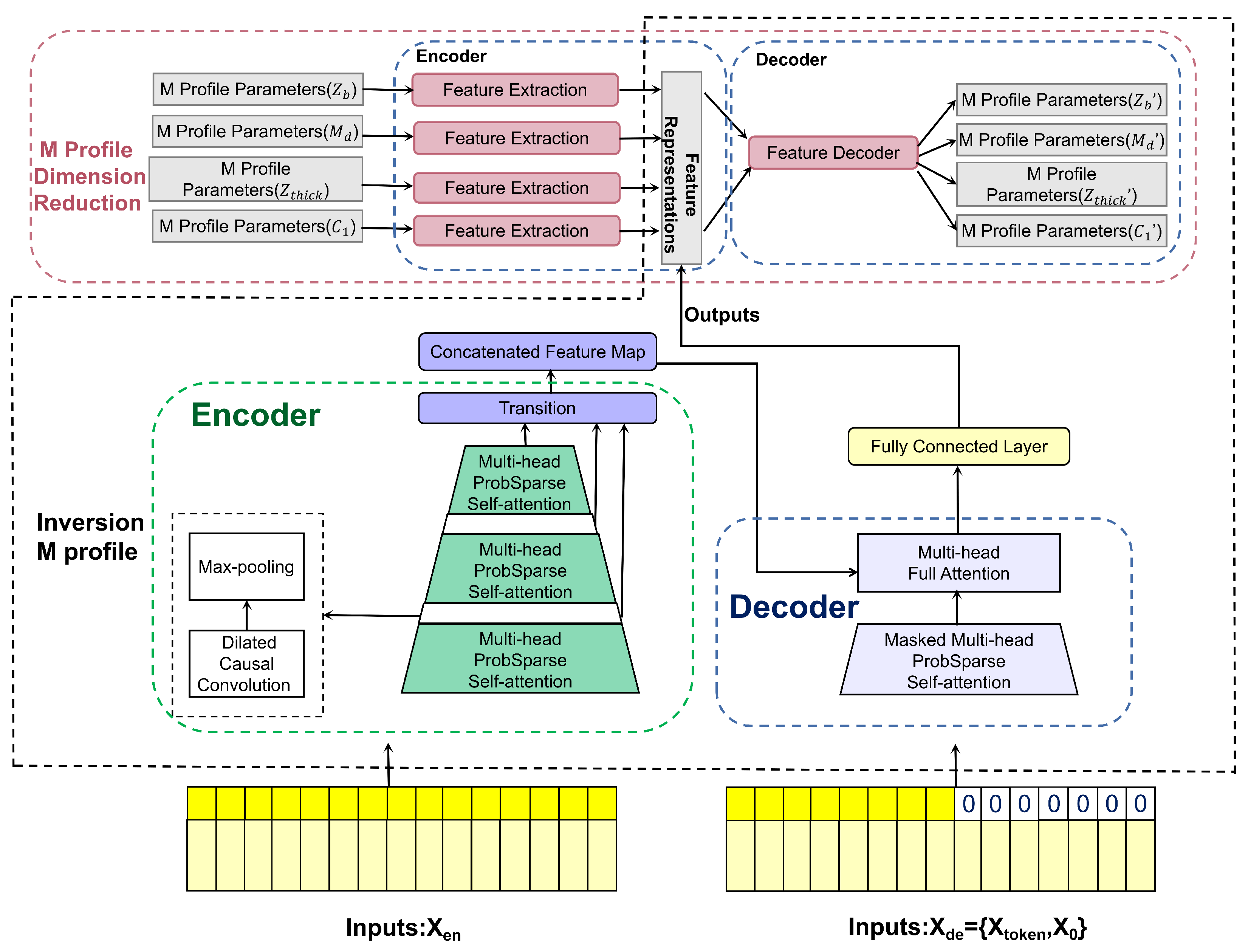
The inversion of the M-profile for the surface-based duct is the inverse of the forward analysis of the radar sea clutter. We proposed a full-coupled convolutional Transformer to establish the nonlinear relationship between sea clutter and the low-dimensional feature representations of M-profile parameters. Figure 5 illustrates the overview structure; see the following sections for details.

2.4.1. Input Representation

To accommodate the dimensionality of our input to the model, an input transformation layer is given at the beginning of the encoder and decoder. Since the Transformer model itself does not have a distance label for the SBD M-profile inversion; we employ a linear operation to embed the learnable position to give positional information. We have taken the clutter power $x^L$ of length L-th as input, the global length stamp of the clutter power range, and the feature dimension after input representation is $d_{\mathrm{model}}$. We first preserve local contextual information by employing a fixed position embedding:

$$\begin{array}{cc}\hfill {\mathrm{PE}}_{\left(\mathrm{pos},2k\right)}& =sin(\mathrm{pos}/{\left(2S_x\right)}^{2k/d_{\mathrm{model}}})\hfill \end{array}$$

(20)

$$\begin{array}{cc}\hfill {\mathrm{PE}}_{\left(\mathrm{pos},2k+1\right)}& =cos(\mathrm{pos}/{\left(2S_x\right)}^{2k/d_{\mathrm{model}}}),\hfill \end{array}$$

(21)

where $k\in \{1,\dots ,[d_{\mathrm{model}}/2]\}$. The range of the clutter power length stamp is employed by a learnable stamp embedding ${\mathrm{SE}}_{\left(\mathrm{pos}\right)}$. To align the dimensions, we project the scalar context $x_i^L$ into $d_{\mathrm{model}}$-dim vector $w_i^L$ with a 1D convolutional filter (kernel width $=3$, stride $=1$). Thus, the input feeding vector is as follows:

$$x_{\mathrm{feed}\left[i\right]}^L=\partial w_i^L+{\mathrm{PE}}_{\left(T_x\times \left(l-1\right)+i\right)}+{\mathrm{SE}}_{(T_x\times \left(l-1\right)+i)},$$

(22)

where $i\in \{1,\dots ,T_x\}$, and ∂ is a factor that balances the size between the scalar projection and the local/global embedding.

2.4.2. Multi-Head-Attention Mechanisms

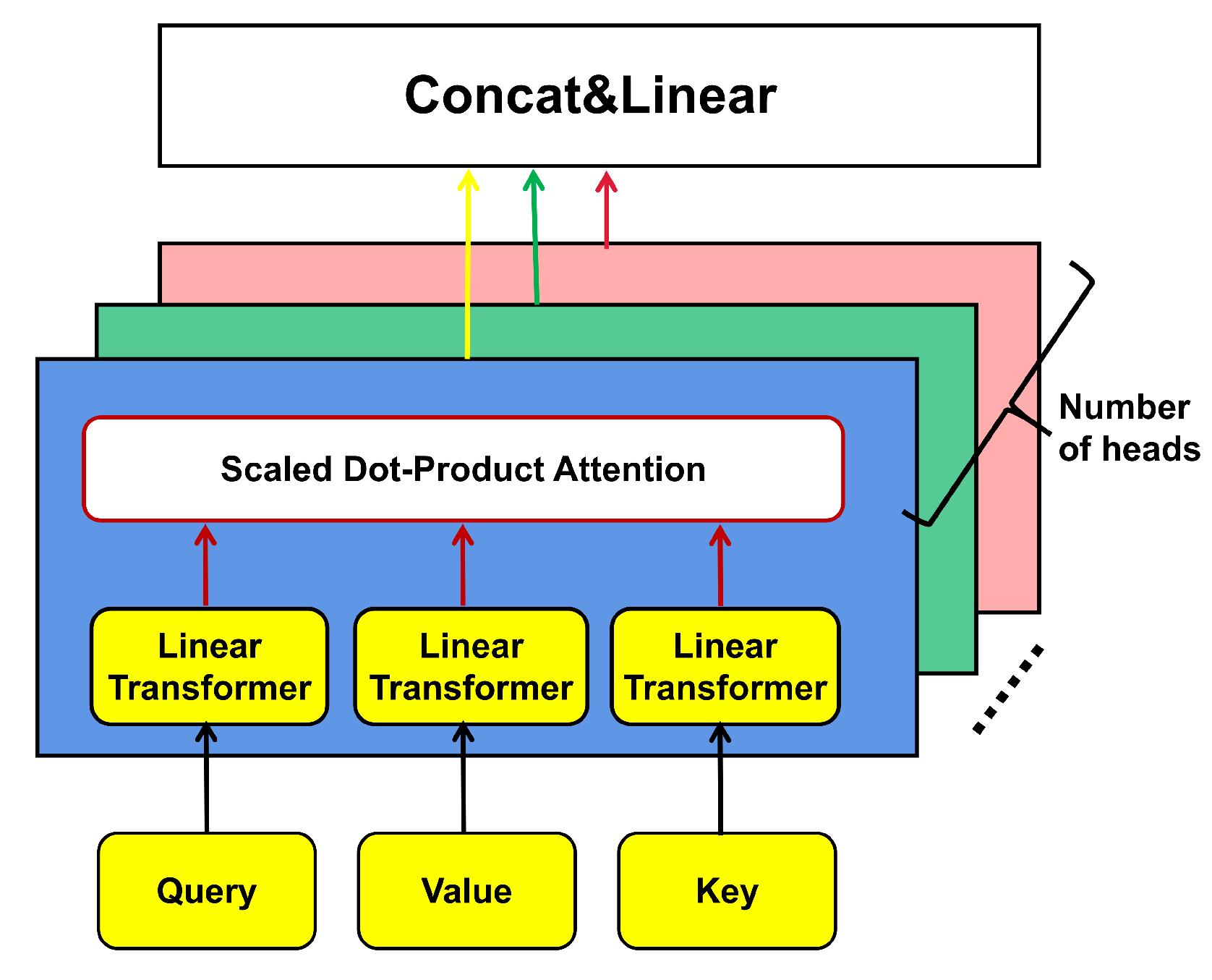
Attention mechanisms in the fields of image and natural language processing represent focusing attention on certain words or target regions in an image. In other words, the attention mechanism is a weighted sum mechanism that assigns different weights to different positions; that is, to give more important positions of clutter power larger weights. Assume that we have canonical attention defined based on a set of key-value pairs $\left(k,v\right)$ and queries $\left(q\right)$ in which the dimensions of keys, values, and queries are $d_k$, $d_v$, and $d_q$, respectively. By weighing the similarity between the queries and keys, the weights are assigned to the values; then the output can be described as:

$$ATTN\left(Q,K,V\right)=f\left(Similarity\left(Q,K\right),V\right),$$

(23)

where Q indicates a matrix by packing a set of queries (vector q), K indicates a matrix by packing a set of keys (vector k), and V indicates a matrix by packing a set of values (vector v).

Vaswani Transformer performs the scaled dot-product attention as follows:

$$ATTN\left(Q,K,V\right)=softmax\left(\frac{Q{K}^T}{\sqrt{d_k}}\right)V.$$

(24)

However, traversing all the queries for measuring $M\left(q_i,K\right)$ requires calculating each dot-product pair. Instead of the Vaswani Transformer self-attention mechanism, ProbSparse self-attention allows each key to focus on the dominant query when performing a scaled dot product. The way to judge the dominant query is through the Kullback–Leibler divergence and uniform distribution of the query-key attention probability distribution. Queries with larger KL divergences are considered to be more dominant. Due to the long-tailed distribution of self-attention scores, ProbSparse self-attention only needs to compute $O\left(ln{L}_Q\right)$ dot-product in typical self-attention instead of $O\left(L_Q\right)$. By ProbSparse self-attention, the model can simultaneously focus on different features from multiple subspace representations. The outputs from each head will be connected and then followed by a linear transformation operation. Figure 6 illustrates muti-head attention work steps. The pseudocode of ProbSparse multi-head attention is exhibited in Algorithm 1.

Algorithm 1: Pseudocode of ProbSparse Multi-Head-Attention

Input Require: $\mathit{Q}\in {\mathit{R}}^{\mathit{m}\times \mathit{d}},\mathit{K}\in {\mathit{R}}^{\mathit{m}\times \mathit{d}},\mathit{V}\in {\mathit{R}}^{\mathit{n}\times \mathit{d}}$   Output    :${\mathit{O}}_{\mathit{attn}}$   Hyper-Parameters: $\mathit{c},\mathit{u}=\mathit{c}\mathbf{ln}\mathit{m},\mathit{U}=\mathit{m}\mathbf{ln}\mathit{n}$, h: number of heads 1 randomly selected $\mathit{U}$ dot-product pairs from $\mathit{K}$ as $\overline{\mathit{K}}$ 2 set the sample score $\overline{\mathit{S}}=\mathit{Q}{\overline{\mathit{K}}}^{\mathit{T}}$ 3 compute the measurement $\mathit{M}=\mathbf{max}\left(\overline{S}\right)-\mathbf{mean}\left(\overline{S}\right)$ by row 4 set Top-$\mathit{u}$ queries under M as $\overline{\mathit{Q}}$ 5 set ${\mathit{S}}_{\mathit{1}}=\mathbf{softmax}\left(\overline{\mathit{Q}}{\mathit{K}}^{\mathit{T}}/\sqrt{\mathit{d}}\right)·\mathit{V}$ 6 set ${\mathit{S}}_{\mathit{0}}=\mathbf{mean}\left(\mathit{V}\right)$ 7 set $\mathit{attn}=\{S_{\mathbf{1}},S_{\mathbf{0}}\}$ by their initial rows 8 ${\mathit{O}}_{\mathit{attn}}=\mathit{W}·\mathbf{concat}({\mathit{attn}}_{\mathbf{1}}+{\mathit{attn}}_{\mathbf{2}}+\dots +{\mathit{attn}}_{\mathbf{h}})$ 9 return ${\mathit{O}}_{\mathit{attn}}$

2.4.3. Encoder for Processing Longer Length Ranges Clutter Power Inputs

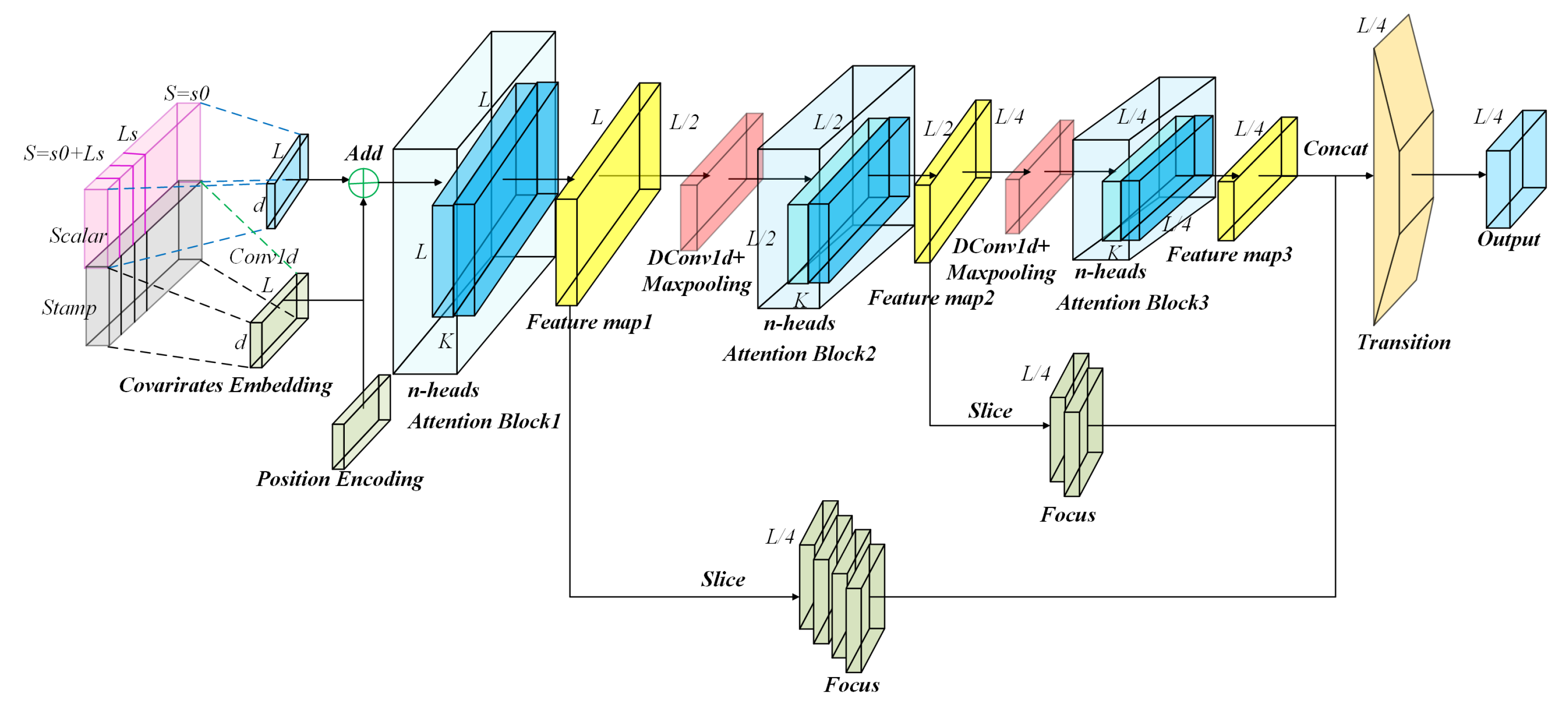
The encoder is designed to extract robustness against long-range SBD clutter power inputs in the range direction. To illustrate this part more clearly, we give a sketch of an encoder in Figure 7.

(1) Self-attention distilling with dilated causal convolution:

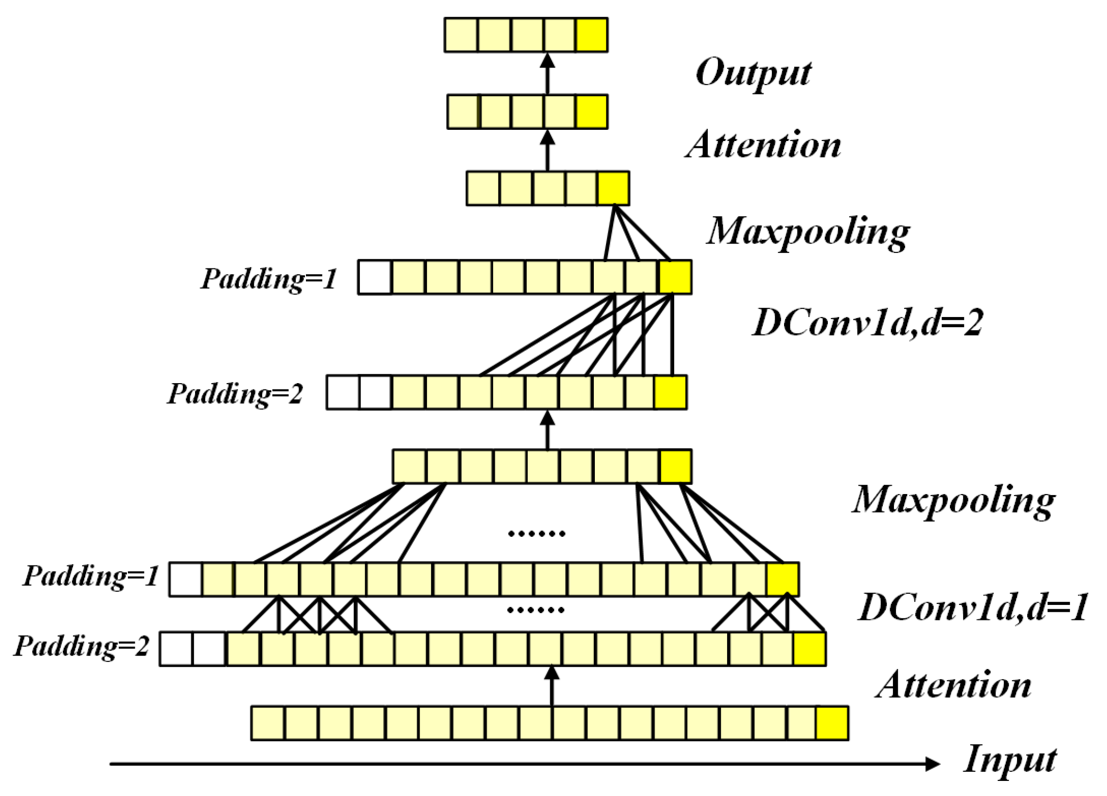
The Vaswani Transformer obtains deeper feature maps by stacking multiple self-attention blocks through fully connected layers, but it will bring more time and space complexity. To further reduce the complexity of the Vaswani Transformer model, the Informer employs a convolutional layer and a max-pooling layer between the two self-attention modules to prune the input length. However, when canonical convolutional layers are applied to the SBD M-profile inversion, the canonical convolutional neural network can only capably review the linear size history as the depth network grows. Therefore, it is not enough to handle the long sequences of clutter power. Moreover, the canonical convolutional network layer does not consider the range perspective of the clutter power, which will inevitably lead to information leakage in the inversion of the range direction sequence. To address this problem, we use dilate causal convolutions to replace traditional convolutional networks. For the $j\mathrm{th}$ convolutional layer following the $j\mathrm{th}$ attention block, the dilated causal convolutional operation DConv1d of kernel size h on the $x_n\in R^d$, $n\in L$ of the input clutter power $X\in R^{L\times d}$ is defined as

$$\mathrm{DConv}1\mathrm{d}\left(x_n\right)=\left[\begin{array}{c}{x}_n\\ x_{n-k}\\ ⋮\\ x_{n-(h-1)\times k}\end{array}\right]W^{m\times m_{\mathrm{out}}},$$

(25)

where $m_{\mathrm{out}}$ is the output dimension, and k is the dilation factor. When $k=1$, the dilated causal convolution is degraded to canonical causal convolution.

As illustrated in Figure 8, we can clearly notice that dilated causal convolution used padding on the temporary front side to prevent future information leakage. Benefitting from the dilated causal convolution, our “self-attention distilling” procedure from the n-th layer to the $(n+1)$-th layer as:

$$x_{n+1}=\mathrm{MaxPool}\left(\mathrm{ELU}\left(\mathrm{DConv}1\mathrm{d}\left(x_n\right)\right)\right),$$

(26)

where DConv1d(.) indicates an 1D convolutional filters (kernel size $=3$) with the ELU(.) activation function. We add a max-pooling layer with stride 2 that is then used to downsample x into its half slice after stacking a layer and providing a less but more focused feature map for the following attention block.

(2) Focus mechanism:

The focus mechanism, proposed by the YoloV5 object-detection CNN network, takes feature maps from the previous network and concatenates them with the final feature map to get more fine-grained clutter power without affecting the model’s parameters. As shown in Figure 9, to perform the inversion of the SBD M-profile from all different global and local scales, we employed a focus mechanism to merge different scales of the clutter power feature maps in a Transformer network. Suppose an encoder stack with n self-attention blocks; each self-attention block would produce a feature map of clutter power. To integrate all the different characteristic maps of clutter power from a more fine-grained perspective, we divide the $Q\mathrm{th}$ feature map into $2^{n-Q}$ feature maps with a length $1/2^{n-1}$. Then, we concatenate all the splice feature maps by dimension, which was calculated by $\left(2^{n-1}\right)\times d$. Moreover, we employ a transition layer to ensure the whole output global feature map has appropriate dimensions.

2.4.4. Decoder: Generating SBD M-Profile Parameter Outputs by Forward Procedure

The decoder network structure consists of four sub-layers: feed the decoder inputs, masked muti-head ProbSparse self-attention layers, encoder and decoder attention layers, and a fully connected layer.

We feed the decoder network with the following clutter power vectors as

$$X_{\mathrm{decoder}}=Concat(X_{\mathrm{token}},X_0)\in R^{(L_{\mathrm{token}}+L_y)\times d_{\mathrm{model}}},$$

(27)

where $X_{\mathrm{token}}\in R^{(L_{\mathrm{token}}+L_y)\times d_{\mathrm{model}}}$ is the start of the token, $X_0\in R^{L_y\times d_{\mathrm{model}}}$ indicates a placeholder for the target SBD M-profile sequence, which sets the scalar as 0.

A masked muti-head ProbSparse self-attention layer constructs a long-range dependence position inside a decoder, which can avoid network auto-regression. An encoder-decoder attention layer constructs long-range dependence between the encoder and the inputs of the decoder. A fully connected network is employed to output the last decoder layer, followed by linear transformation. The output of the last decoder layer, followed by linear transformation, is the final SBD M-profile parameter inversion. For performance evaluation, we employ the MAE and RMSE loss functions on the inversion of the target SBD M-profile parameters.

2.4.5. One-dimensional-RDCAE Decoder Network: Reconstructing Full-Space SBD M-Profile

The low-degree-of-freedom feature representation SBD M-profile parameter matrices output by the FCCT is used as the input to the decoder network of the 1D-RDCAE. The decoder network includes a bottleneck layer, four deconvolutional layers, and four upsampling layers. The size of the first, second, third, and fourth deconvolution layers was set to 12, 62, 250, and 1000, respectively. According to the decoder network, a full-space SBD M-profile parameter matrix is reconstructed to realize its high-dimension inversion.

In this paper, we employ MAE and RMSE as loss functions and design the following three training strategies. First, we want to show the effectiveness and necessity of the 1D-RDCAE for feature extraction from an inhomogeneous surface-based duct. Thus, we evaluate the 1D-RDCAE and benchmarks and compare their performance by using root mean square error (RMSE), mean absolute error (MAE), and R-square ($R^2$). RMSE and MAE indicate the accuracy of the inversion model. The smaller the value is, the higher the accuracy is. $R^2$ is used for linear regression to represent the number of variables described by the regression. If the value is 1, the model perfectly predicts the value of the target variable. For further comparisons of the FCCT method with state-of-the-art Transformer-based models, we employed 5-fold and 10-fold cross-validation MAE, model parameters, running time, and calculation complex, five times to verify the inversion model. Finally, to verify the effectiveness of the proposed FCCT deep learning model using the measured data, we used the radar sea clutter power data measured in the Wallops’98 experiment in the United States to invert and verify the inhomogeneous surface-based duct M-profile [9].

3. Results and Discussion

3.1. Dataset

The data used for the experiments on dimension reduction from the SBD M-profiles comprised 5000 sets of parameters, including the height of the base, the thickness of the trapping layer, the refractive index of the trapping layer, and the slope of the base layer for a range of 0–100 km and a range interval of 0.1 km simulated with the aid of a Markov chain. The clutter power for the inversion SBD M-profile experiments includes 5000 sets of data computed by bringing SBD M-profile parameters into PE and radar sea clutter formulas. The train/val is 80%/20% data sample by default. The accuracy of the inversion model was validated using two sets of simulated sea clutter power data and four sets of measured sea clutter power [9]. The parameters of the radar system applied in the calculation are shown in

Table 2. Radar properties.

Parameter	Value
Radar Transmitting Frequency (GHz)	2.84
Power (dBm)	91.40
Antenna gain (dB)	52.80
Polarization Mode	VV
Antenna Height (m)	30.78
Antenna elevation angle (deg)	0.0
Beam Width (${}^{\circ }$)	0.39
Distance resolution (m)	600

.

The computer system used in the experiments was a Windows Server 2016 Standard with Intel (R) Xeon(R) CPU E5-2650 [email protected] GHz and two GPUs named TESLA.

3.2. One-dimensional-RDCAE Used for SBD M-Profile Dimension Reduction

The network structure and parameters setup of the 1D-RDCAE are presented in

Table 3. 1D-RDCAE structure.

Layer	Value
Dconvolutional 1	Kernel Size $=2$, Filter $=128$
Max-pooling 1&2&3&4	Strides $=4$, Pooling Size $=4$
Dconvolutional 2	Kernel Size $=2$, Filter $=64$
Dconvolutional 3	Strides $=2$, Filter $=16$
Dconvolutional 4	Strides $=2$, Filter $=8$
Bottleneck 1&2	Strides $=2$, Filter $=8$
DeDconvolution 1	Strides $=2$, Filter $=8$
Upsampling 1&2&3&4	Strides $=4$, Pooling Size $=4$
DeDconvolution2	Strides $=2$, Filter $=16$
DeDconvolution3	Strides $=2$, Filter $=64$
DeDconvolution4	Strides $=2$, Filter $=128$
Flatten& Fully Connected	Units $=1000$
Learning Rate	0.0001
Batch Size	256

. The four dilated causal convolution kernel layers, and one bottleneck layer reduce the M-profile parameters of the 1000-dimension range direction set to 250, 62, and 15 to 3 degrees of freedom. In parallel, one bottleneck layer, four de-dilated causal convolution kernel layers, and one fully connected layer reconstruct the SBD M-profile.

3.2.1. One-dimensional-RDCAE Parameter Analysis

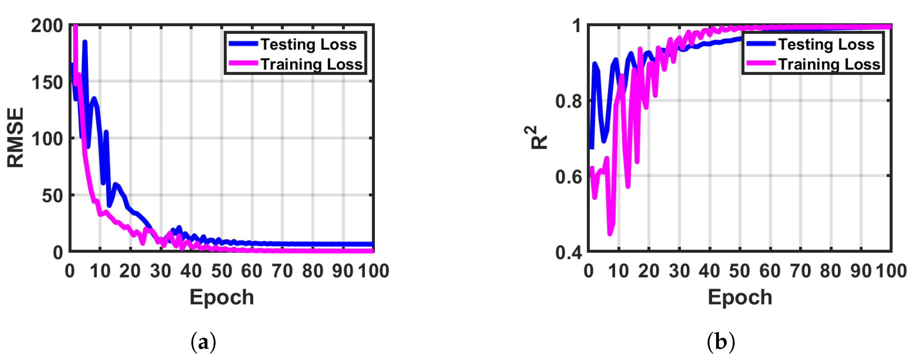
Figure 10 shows the RMSE and $R^2$ during the 1D-RDCAE model testing and training phases. While the number of the training epochs increases, the RMSE consistently converges. To further verify the accuracy of the network training and testing, we use $R^2$, which is employed in linear regression to represent the number of variables described by the regression. If the value is one, the model perfectly predicts the value of the target variable. As illustrated in Figure 10b, the model converges to one with the increase in the number of epochs.

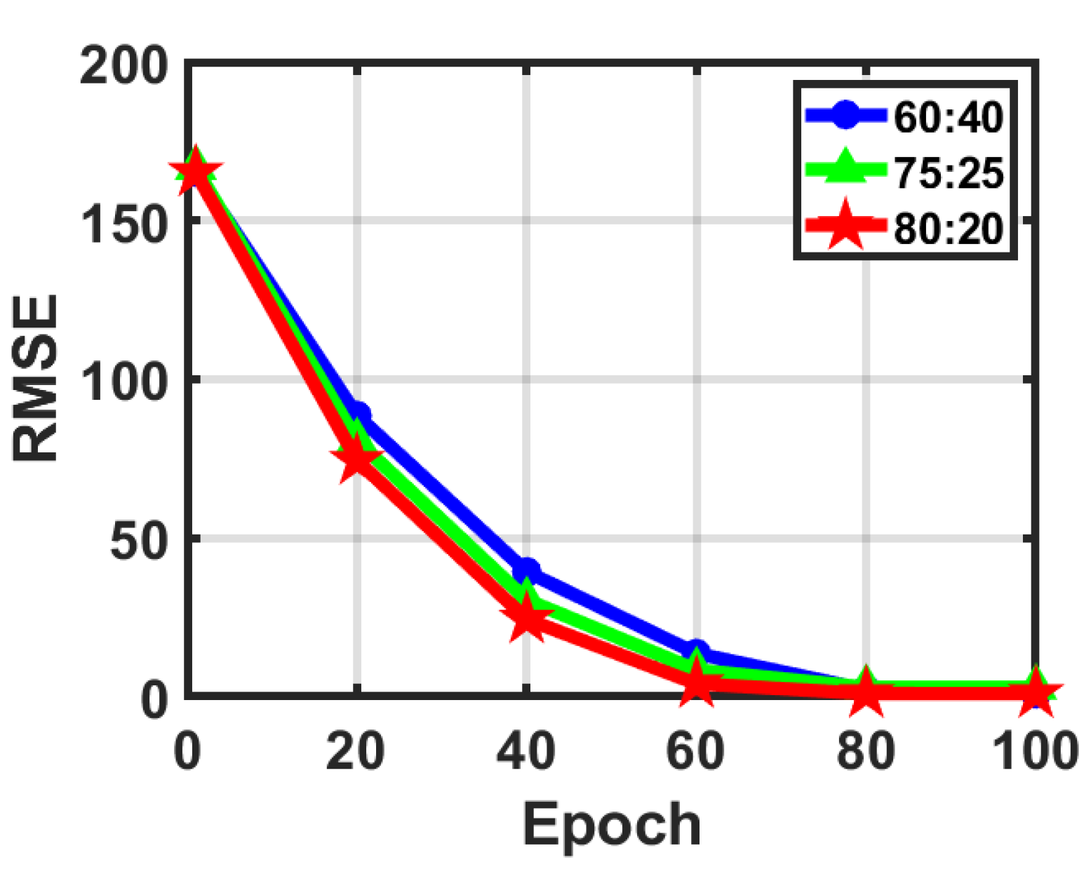
In the process of model training, the reasonable division of datasets will have an important impact on the model training. The division of the training/test set should be as consistent as possible in terms of the data distribution to avoid additional biases introduced by the data partitioning process that affect the final result. As shown in Figure 11, we compare the RMSE of the three classical training/testing set division ratios of 60:40, 75:25, and 80:20 in the model’s training and tuning phases. These results indicate that the training/testing ratio of 80:20 converges faster and more accurately than the other two ratios. Therefore, the training and test datasets of this article are divided into 80:20.

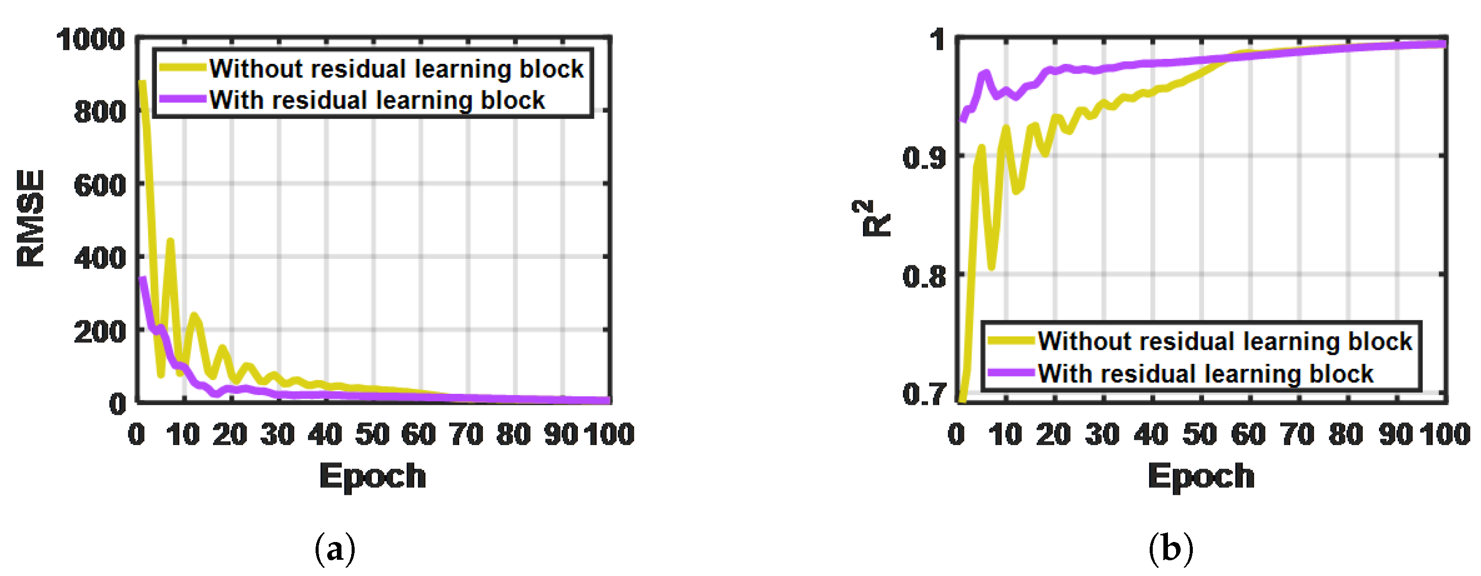
The residual learning block plays an essential part in the 1D-RDCAE network. As indicated in Figure 12, while the number of epochs increases, the model with the residual learning block converges asymptotically, whereas the one without the residual learning block exhibits an obvious oscillation and a slower systematic convergence.

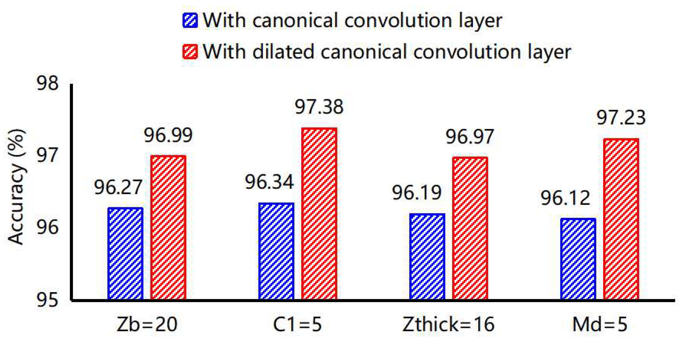
As demonstrated in Figure 13, we compare the average accuracy of the M-profile of each parameter with a canonical convolution layer and a dilated causal convolution layer. It is obvious that the model with a dilated causal convolution layer reconstructs the original M-profile parameters more accurately. The result clearly demonstrates the effectiveness and necessity of the dilated causal convolution for feature extraction from inhomogeneous surface-based ducts.

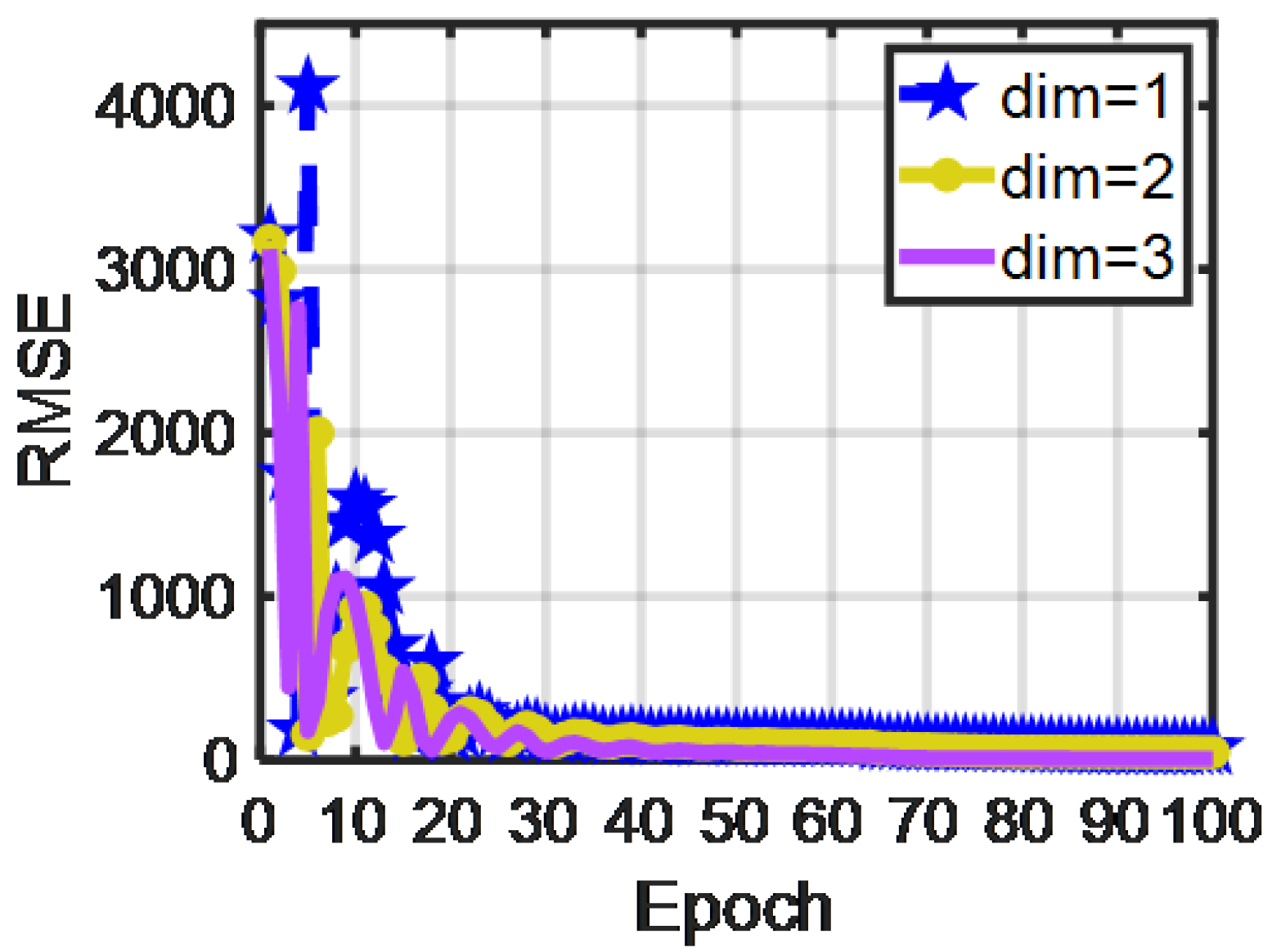
The final dimensions of the feature extraction model affect the accuracy of the reconstructed M-profile. As demonstrated in Figure 14, we compare the RMSE of the training and tuning phases with target dimensions of one, two, and three. These results illustrate that a faster convergence rate is achieved for a target dimension of three than for a target dimension of one or two, and the RMSE in the latter cases is not as small as in the three-dimensional case. This indicates that when the dimension is increased to three, 1D-RDCAE can achieve more accurate data reconstruction.

3.2.2. Comparisons of Dimensional Reduction Results

In this section, we first compare the proposed method with the traditional PCA method. To further verify the effectiveness of our proposed method, we compare the classical dimensionality reduction models in the field of deep learning.

As demonstrated in

Table 4. The performance of 1D-RDCAE and baseline methods.

Model		Dimension $=2$				Dimension $=3$
		RMSE	MAE	${\mathit{R}}^2$	Time (s)	RMSE	MAE	${\mathit{R}}^2$	Time (s)
	PCA	3.62	2.47	0.91	48	3.57	2.38	0.92	49
	BPN	0.72	0.61	0.94	43	0.51	0.41	0.95	43
	SAE	0.69	0.59	0.94	43	0.44	0.35	0.95	42
Zb = 20	DBN	0.56	0.51	0.95	43	0.38	0.31	0.96	42
	1D-CAE	0.49	0.49	0.95	41	0.36	0.33	0.97	40
	1D-RCAE	0.35	0.39	0.96	40	0.28	0.29	0.97	39
	1D-RDCAE	0.32	0.29	0.97	40	0.23	0.22	0.98	39

, 1D-RDCAE achieved the best performance in terms of all the evaluated metrics.

For the PCA, when the target dimension increased from 2 to 3, the RMSE, MAE, and $R^2$ did not significantly change. Considering that the PCA merely discards some features by approximation and does not consider any information related to the outcome parameters, the most significant features may be lost. For the BPN, SAE, and DBN models, when the target dimension increased, the RMSE, MAE and $R^2$ first decreased. Notwithstanding that the accuracy of dimension reduction can be enhanced by increasing the number of dimensions, this improvement is insufficient to simulate larger datasets because its inherent fully connected architecture engenders overfitting and high computational cost during the training of the network. Regarding 1D-CAE, 1D-RCAE, and 1D-RDCAE, when the target dimensions increased, the results of the three models exhibited considerably better precision. Compared with 1D-CAE and 1D-RCAE, the 1D-RDCAE model can process the original data more meticulously and achieves the best performance. Thus, our proposed model achieved excellent results, and the reconstructed output data were identical to the original sample data.

3.3. FCCT Used for Inversion SBD M-Profile Parameters

3.3.1. FCCT Parameters

The details of the proposed FCCT structure are summarized in

Table 5. The full-coupled convolutional Transformer network components in detail.

Encoder:
Input	$1\times$ 3Conv1d	Embedding ($d=128$)
ProbSparse Self-attention Block	Multi-head ProbSparse Attention ($h=8$, $d=32$)
	Add Layer Norm, Dropout($p=0.1$)
	FFN (dinner $=256$), GELU
	Dropout ($p=0.1$)
Distilling	$1\times$ 3DeConv1d, BatchNorm1d, ELU($p=0.1$), Dropout($p=0.1$),
	Maxpooling (Kernel size $=1$, stride $=2$, padding $=1$)
Focus Layer	$1\times$ 3Conv1d, BatchNorm1d
Decoder:
Input	$1\times$ 3Conv1d	Embedding ($d=128$)
Masked Layer	Add Mask on Attention Block
ProbSparse Self-attention Block	Multi-head ProbSparse Attention ($h=8$, $d=32$)
	Add, Layer Norm, Dropout($p=0.1$)
	FFN (dinner $=256$), GELU
	Add, Layer Norm, Dropout ($p=0.1$)
Final:
Output	Fully Connected & Reshape($4\times (2000,3)$)
Learning Rate	0.0001

. For the input layer, to align the dimension, we embed the input data into a 512-dim vector with 1D convolutional filters (kernel size $=3$, stride $=1$). For the ProbSparse self-attention block, we let $d=32$ and $n=8$, and add residual connections, a feed-forward network layer (inner-layer dimension is 256) and a dropout layer ($p=0.1$). Between every-two ProbSparse Self-attention blocks, a dilated causal convolutional layer and a maxpooling layer are used for connection; we set ELU ($p=0.1$) and Dropout ($p=0.1$). We employ a focus layer to merge different feature maps in the Transformer network; we set the kernel size $=3$ and stride $=1$.

3.3.2. Comparisons of SBD M-Profile Inversion Results

To verify the effectiveness of the deep learning inversion model, we first compare DNN with four classic machine learning inversion models based on a set of simulated clutter power data. The results of the model are shown in

Table 6. Comparison of classical inhomogeneous inversion models.

Model	Year	${\mathit{z}}_{\mathit{b}}$	${\mathit{c}}_1$	${\mathit{z}}_{\mathbf{thick}}$	${\mathit{M}}_{\mathit{d}}$	Time (s)
GA [9]	2003	90.95	91.27	90.32	90.37	155512
PSO [5]	2012	91.34	91.56	92.31	91.39	136753
SVM [29]	2013	91.25	91.93	92.12	91.56	927
MLP [30]	2018	91.29	91.99	92.93	92.09	759
BPNN [18]	2020	93.92	92.32	93.96	94.03	682
DNN [19]	2022	94.59	94.97	95.29	95.31	697

. The DNN model is superior to the traditional GA, PSO, SVM, and MLP algorithms in terms of time and final accuracy of the task. Using the same 16 hidden layers and model hyperparameters, the accuracy and running time of the DNN model are better than the BPNN model.

For the fair comparison of our proposed method with state-of-the-art Transformer-based models, we employed 5-fold and 10-fold cross-validation methods, model parameters, running time, and calculation complex, five times to verify the inversion model. For the default training settings, which are widely adopted in classic Transformers, we use standard preprocessing to train the network for approximately 200 epochs, all models are trained using the same dataset. Specifically, all the hyperparameters are set to this in the official implementation without any additional adjustments.

Similarly, our proposed FCCT model is trained in an end-to-end style. We set the batch size to 128.

Although DNN can achieve a relatively high accuracy compared with the other classical methods, it is still unable to achieve significant results in the inversion of the high-dimensional M-profile. As demonstrated in

Table 7. Comparison of deep learning models.

Model	MAE $\mathit{K}=5$	MAE $\mathit{K}=10$	Params (M)	GFLOPS (G)	Time (s)
DNN [19]	5.71	2.69	563.91	0.86	697
Transformer [23]	0.84	0.67	9.932	2.931	681
LogTrans [31]	0.83	0.67	9.821	2.832	569
INFORMER [21]	0.57	0.46	6.358	2.759	539
FCCT	0.47	0.37	6.028	2.532	491

, in the five- and ten-fold MAE cross-validation on simulated datasets, our proposed FCCT network obtains better performance compared to the other state-of-the-art Transformer-based models, including its runtime and lightweight model parameters. Specifically, in DNN models, as the number of network layers increases, excessive network parameters in the training process make the model require plenty of training time and memory consumption, which seriously affects its efficiency. Transformer has better performance than the DNN model, but the performance of Transformer and other state-of-the-art models are still lower than the stronger Transformer-based FCCT structure that strengthens the capacity to elaborate upon the multi-head attention, self-attention distilling with dilated causal convolutional, and focus mechanism design of SBD M-profile.

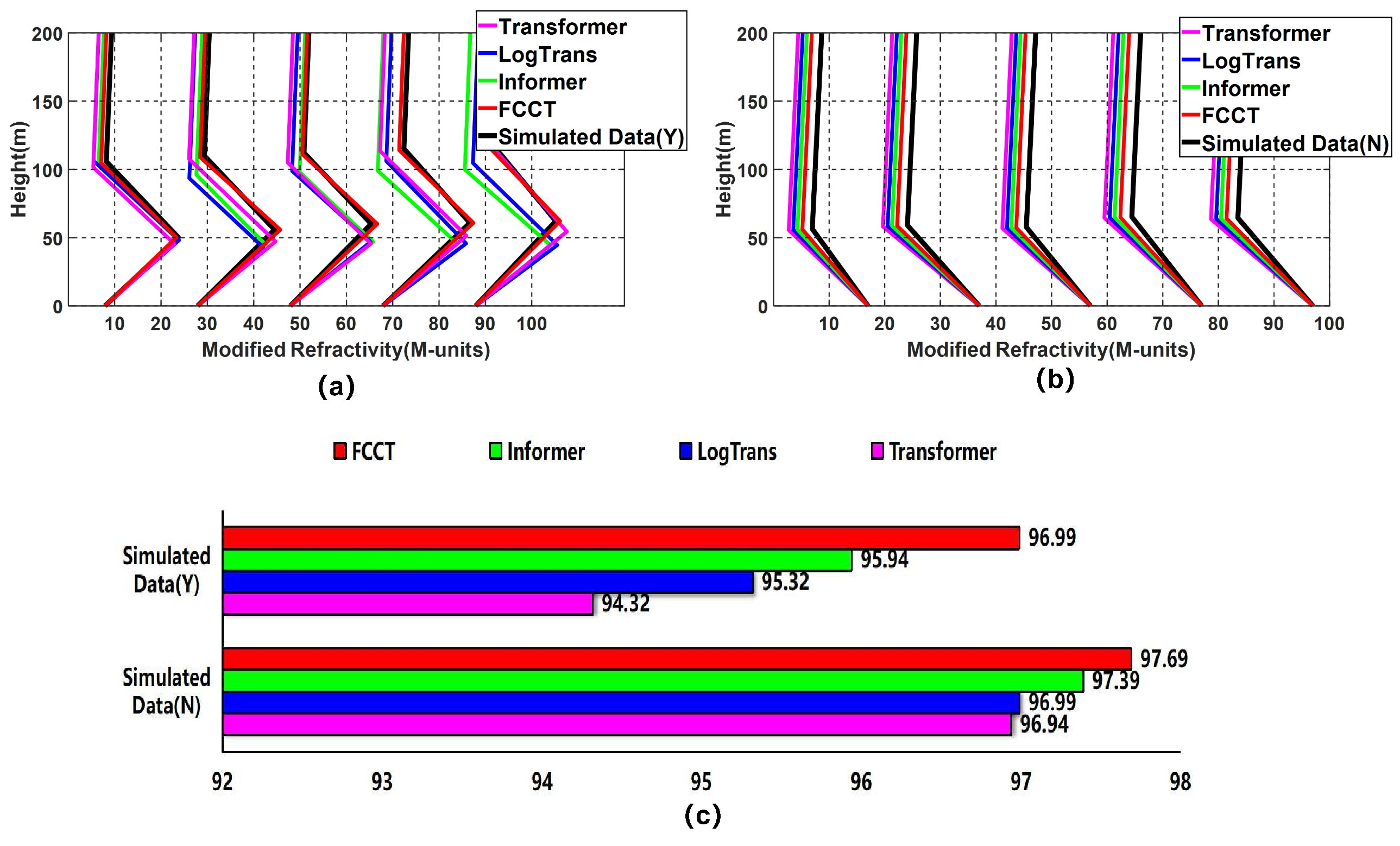
As shown in Figure 15, we compare our proposed FCCT model with other state-of-the-art Transformer-based methods using two sets of simulated clutter power data. First, it is easily observable that our proposed inversion method is more consistent with the reference simulated data and achieves the best performance. Second, the inversion of the two sets of simulated sea clutter power data reached 96.99% and 97.69%, which reflects the benefit of using the tailored inversion method of surface-based duct M-profile.

3.3.3. Measured Data Inversion Results

To verify the effectiveness of the proposed FCCT deep learning model, we used the radar sea clutter power data measured in the Wallops’98 experiment in the United States to invert and verify the inhomogeneous surface-based duct M-profile.

Detailed descriptions of Wallops’98 experiments and data can be found in Refs. [9] and [32], this section mainly presents a brief introduction to the data used in this paper. The Wallops’98 experiment used the reception and processing of sea clutter data by Space Range Radar (SPANDAR). The system parameters of the radar are shown in Table 1.

To verify the effectiveness of the proposed deep learning FCCT model, we used the trained inversion model and the same computer hardware conditions; all inversion results can be completed within 5 s, and the measured sea clutter profile (12:50 UT, 13:00 UT, 13:40 UT, and 14:00 UT from top to bottom, respectively) are marked in blue, the inversion refractive index profile and the inverted clutter power profile are marked in red, the refractive index M-profile of a helicopter (from top to bottom corresponds to 12:26 UT-12:50 UT, 12:52 UT-13:17 UT, 13:19 UT-13:49 UT, and 13:51 UT-14:14 UT, respectively) and the clutter power profile of the helicopter is marked in blue.

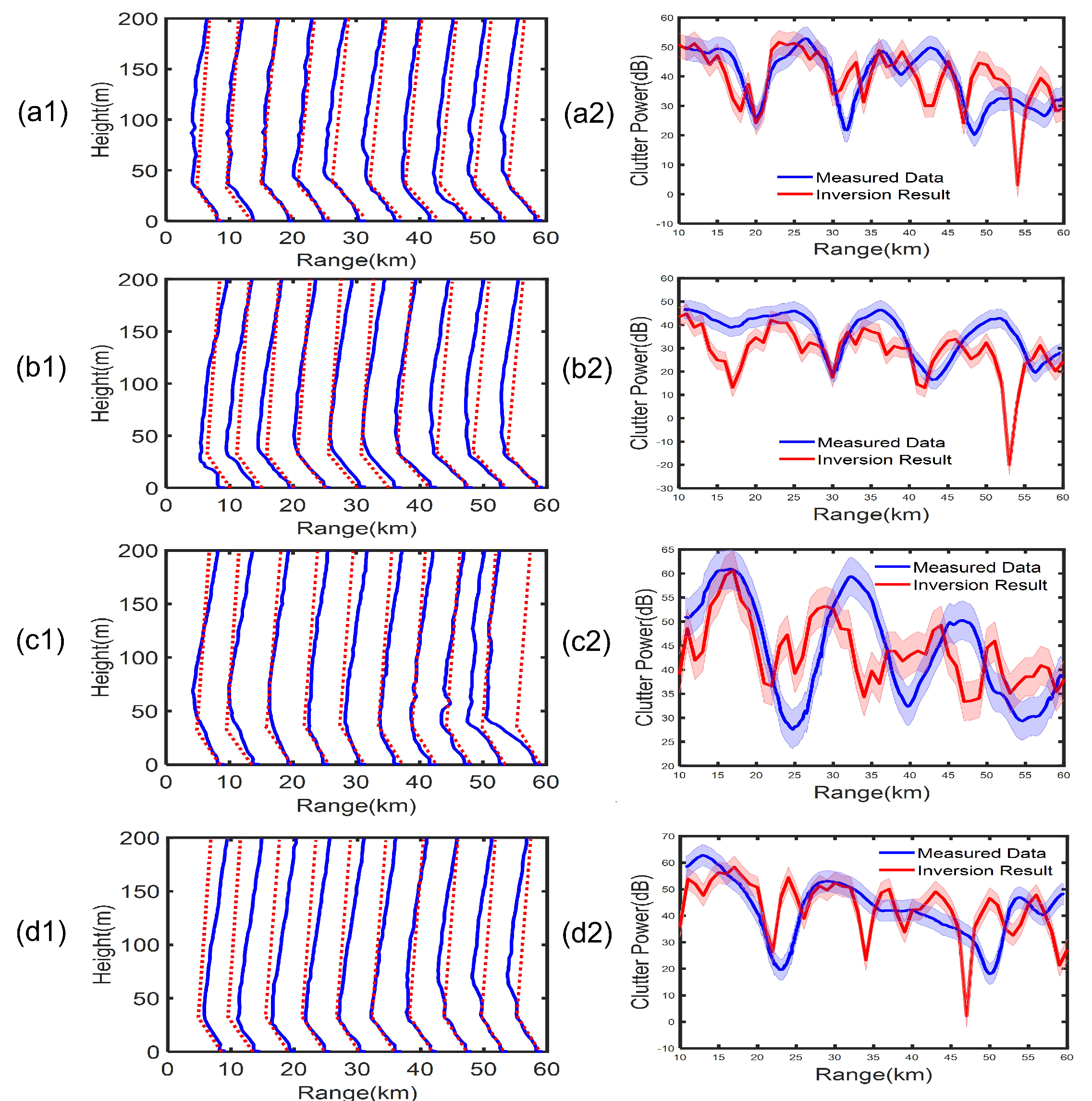
It can be clearly concluded from the left column of Figure 16 that the modified refractive index profile of the inversion can reflect the profile characteristics of the surface-based duct structure observed by the helicopter as a function of distance. However, the inversion and measured profiles do not exactly match each other. The main reason for this phenomenon is that the refractive index profiles of each group of helicopters were observed over a time frame of 25 min, but the inverted profiles reflect the instantaneous refractive index profile information corresponding to each clutter measurement.

In the right column of Figure 16, the calculated clutter power based on the inverted refractive index profile basically agrees with the observed results, but there are still some errors. The inversion power of a2 and d2 are in good agreement with the measured power; however, the measured power of c2 is in poor agreement with the measured power, because, for the propagation of tropospheric electromagnetic waves, the propagation characteristics are mainly determined by the refraction conditions. The c2 invention refractive index structure is in error with the measured refractive index structure; however, small differences can lead to large errors in EM propagation simulations. From the comparison of the overall clutter power of the four groups, it can be inferred that the inversion results of the four groups are basically consistent with the information of the refractive index profile and the information of the sea clutter power profile, indicating the effectiveness and stability of the proposed method.

4. Conclusions

When inverting high-dimension inhomogeneous SBD M-profile parameters, the classic GA and PSO models render low productivity and large errors. To tackle these problems, a deep-learning model for addressing the computational complexity and large inversion errors of the SBD M-profile was proposed. Specifically, we first proposed a one-dimensional residual dilated causal convolutional autoencoder (1D-RDCAE) to extract the SBD M-profile feature representations from high-dimension range-direction M-profiles. Second, the inversion efficiency and precision were enhanced using a fully coupled convolutional Transformer (FCCT) that transforms two CNN architectures into a Transformer model to establish a network mapping between sea clutter and the low-dimensional representative M-profile parameters. To show the advantages of FCCT, we tested its performance on two sets of simulated sea clutter power data where the inversion of the simulated data reached 96.99% and 97.69%, which outperformed the existing baseline methods. To verify the effectiveness of the proposed FCCT deep learning model, we used the radar sea clutter power data measured in the Wallops’98 experiment in the United States to invert and verify the inhomogeneous SBD M-profile. The results show the power of our proposed model; however, it is worth discussing the limitations of the model. As a data-driven model, the FCCT learns the nonlinear relationship between the SBD M-profile and clutter power purely from data. There remains a lack of physical explanations in the inversion process, although we try to explain the entire physical process. Second, the FCCT model has less measured data, so the inversion accuracy of the measured data is not ideal, although we obtained the best inversion results from the simulated data. Therefore, future work will focus more on an explanatory inversion model and conducting more experiments to collect more measured data to continuously improve the accuracy of the model.

References

- Zhang, J. Research on Radar Sea Clutter/GPS Signal Inversion Method for Marine Tropospheric Duct; Xidian University: Xi’an, China, 2012. [Google Scholar]
- Dou, P.; Shen, H.; Li, Z.; Guan, X. Time series remote sensing image classification framework using combination of deep learning and multiple classifiers system. Int. J. Appl. Earth Obs. Geoinf. 2021, 103, 102477. [Google Scholar] [CrossRef]
- Wang, G.; Jia, Q.S.; Zhou, M.; Bi, J.; Qiao, J. Soft-sensing of Wastewater Treatment Process via Deep Belief Network with Event-triggered Learning—ScienceDirect. Neurocomputing 2021, 436, 103–113. [Google Scholar] [CrossRef]
- Yu, J.; Liu, G. Extracting and inserting knowledge into stacked denoising auto-encoders. Neural Netw. 2021, 137, 31–42. [Google Scholar] [CrossRef] [PubMed]
- Paoletti, M.; Haut, J.; Plaza, J.; Plaza, A. A new deep convolutional neural network for fast hyperspectral image classification. ISPRS J. Photogramm. Remote Sens. 2018, 145, 120–147. [Google Scholar] [CrossRef]
- Han, M.; Cong, R.; Li, X.; Fu, H.; Lei, J. Joint spatial-spectral hyperspectral image classification based on convolutional neural network. Pattern Recognit. Lett. 2020, 130, 38–45. [Google Scholar] [CrossRef]
- Dasan, E.; Panneerselvam, I. A novel dimensionality reduction approach for ECG signal via convolutional denoising autoencoder with LSTM. Biomed. Signal Process. Control 2021, 63, 102225. [Google Scholar] [CrossRef]
- Zhang, M.; Gong, M.; Mao, Y.; Li, J.; Wu, Y. Unsupervised Feature Extraction in Hyperspectral Images Based on Wasserstein Generative Adversarial Network. IEEE Trans. Geosci. Remote Sens. 2019, 57, 2669–2688. [Google Scholar] [CrossRef]
- Gerstoft, P.; Rogers, L.T.; Krolik, J.L.; Hodgkiss, W.S. Inversion for refractivity parameters from radar sea clutter. Radio Sci. 2003, 38, 8053. [Google Scholar] [CrossRef]
- Zhang, J.; Zhang, Y.; Wu, Z.; Zhang, Y.; Hu, R. Inversion of regional range-dependent evaporation duct from radar sea clutter. Acta Phys. Sin. 2015, 64, 124101. [Google Scholar] [CrossRef]
- Isaakidis, S.A.; Dimou, I.N.; Xenos, T.D.; Dris, N.A. An artificial neural network predictor for tropospheric surface duct phenomena. Nonlinear Process. Geophys. 2007, 14, 569–573. [Google Scholar] [CrossRef]
- Douvenot, R.; Fabbro, V.; Gerstoft, P.; Bourlier, C.; Saillard, J. A duct mapping method using least squares support vector machines. Radio Seience 2008, 43, 1–12. [Google Scholar] [CrossRef]
- Remi, D.; Vincent, F.; Christophe, B.; Joseph, S.; Hans-Hellmuth, F.; Helmut, E.; Joerg, F. Retrieve the evaporation duct height by least-squares support vector machine algorithm. J. Appl. Remote Sens. 2009, 3, 033503. [Google Scholar]
- Yan, X.; Yang, K.; Ma, Y. Calculation Method for Evaporation Duct Profiles Based on Artificial Neural Network. Antennas Wirel. Propag. Lett. IEEE 2018, 17, 2274–2278. [Google Scholar] [CrossRef]
- Compaleo, J.; Yardim, C.; Xu, L. Refractivity-From-Clutter Capable, Software-Defined, Coherent-on-Receive Marine Radar. Radio Sci. 2021, 56, 1–19. [Google Scholar] [CrossRef]
- Zhou, S.; Gao, H.; Ren, F. Pole Feature Extraction of HF Radar Targets for the Large Complex Ship Based on SPSO and ARMA Model Algorithm. Electronics 2022, 11, 1644. [Google Scholar] [CrossRef]
- Guo, X.; Wu, J.; Zhang, J.; Han, J. Deep learning for solving inversion problem of atmospheric refractivity estimation. Sustain. Cities Soc. 2018, 43, 524–531. [Google Scholar] [CrossRef]
- Zhao, W.; Li, J.; Zhao, J.; Jiang, T.; Zhu, J.; Zhao, D.; Zhao, J. Research on evaporation duct height prediction based on back propagation neural network. IET Microwaves Antennas Propag. 2020, 14, 1547–1554. [Google Scholar] [CrossRef]
- Ji, H.; Yin, B.; Zhang, J.; Zhang, Y. Joint Inversion of Evaporation Duct Based on Radar Sea Clutter and Target Echo Using Deep Learning. Electronics 2022, 11, 2157. [Google Scholar] [CrossRef]
- Lim, B.; Arik, S.O.; Loeff, N.; Pfister, T. Temporal Fusion Transformers for Interpretable Multi-horizon Time Series Forecasting. Int. J. Forecast. 2019, 37, 1748–1764. [Google Scholar] [CrossRef]
- Zhou, H.; Zhang, S.; Peng, J.; Zhang, S.; Li, J.; Xiong, H.; Zhang, W. Informer: Beyond efficient transformer for long sequence time-series forecasting. Proc. AAAI Conf. Artif. Intell. 2021, 35, 11106–11115. [Google Scholar] [CrossRef]
- Yin, H.; Guo, Z.; Zhang, X.; Chen, J.; Zhang, Y. RR-Former: Rainfall-runoff modeling based on Transformer. J. Hydrol. 2022, 609, 127781. [Google Scholar] [CrossRef]
- Vaswani, A.; Shazeer, N.; Parmar, N.; Uszkoreit, J.; Jones, L.; Gomez, A.N.; Kaiser, L.u.; Polosukhin, I. Attention is All you Need. In Proceedings of the Advances in Neural Information Processing Systems, Long Beach, CA, USA, 4–9 December 2017; Guyon, I., Luxburg, U.V., Bengio, S., Wallach, H., Fergus, R., Vishwanathan, S., Garnett, R., Eds.; Curran Associates, Inc.: Red Hook, NY, USA, 2017; Volume 30. [Google Scholar] [CrossRef]
- Shen, L.; Wang, Y. TCCT: Tightly-coupled convolutional transformer on time series forecasting. Neurocomputing 2022, 480, 131–145. [Google Scholar] [CrossRef]
- Liu, M.; Li, Z.; Li, Y.; Liu, Y. A Fast and Accurate Method of Power Line Intelligent Inspection Based on Edge Computing. IEEE Trans. Instrum. Meas. 2022, 71, 1–12. [Google Scholar] [CrossRef]
- He, K.; Zhang, X.; Ren, S.; Sun, J. Deep Residual Learning for Image Recognition. In Proceedings of the IEEE Conference on Computer Vision and Pattern Recognition (CVPR), Las Vegas, NV, USA, 27–30 June 2016; pp. 770–778. [Google Scholar] [CrossRef]
- Bai, S.; Kolter, J.Z.; Koltun, V. An empirical evaluation of generic convolutional and recurrent networks for sequence modeling. arXiv 2018, arXiv:1803.01271. [Google Scholar] [CrossRef]
- Stoller, D.; Tian, M.; Ewert, S.; Dixon, S. Seq-u-net: A one-dimensional causal u-net for efficient sequence modelling. arXiv 2019, arXiv:1911.06393. [Google Scholar]
- Chao, Y. A comparison of the machine learning algorithm for evaporationduct estimation. Radioengineering 2013, 22, 657–661. [Google Scholar] [CrossRef]
- Zhu, X.; Li, J.; Min, Z.; Jiang, Z.; Li, Y. An Evaporation Duct Height Prediction Method Based on Deep Learning. IEEE Geoence Remote Sens. Lett. 2018, 15, 1307–1311. [Google Scholar] [CrossRef]
- Li, S.; Jin, X.; Xuan, Y.; Zhou, X.; Chen, W.; Wang, Y.X.; Yan, X. Enhancing the Locality and Breaking the Memory Bottleneck of Transformer on Time Series Forecasting. In Proceedings of the Advances in Neural Information Processing Systems, Vancouver, BC, Canada, 8–14 December 2019; Wallach, H., Larochelle, H., Beygelzimer, A., d’Alché Buc, F., Fox, E., Garnett, R., Eds.; Curran Associates, Inc.: Red Hook, NY, USA, ; 2019; Volume 32. [Google Scholar]
- Rogers, L.T.; Hattan, C.P.; Stapleton, J.K. Estimating evaporation duct heights from radar sea echo. Radio Sci. 2000, 35, 955–966. [Google Scholar] [CrossRef] [Green Version]
Figure 1.
(a) Three-fold refractive index includes four basic parameters: the height of the base (), the thickness of the trapping layer (), the refractive index of the trapping layer (), and the slope of the base layer (). (b) Two-fold line refractive index M-profile includes two parameters: the thickness of the trapping layer (), and the refractive index of the trapping layer ().
Figure 2.
Parameters of the surface-based duct M-profile modeled with a Markov chain. The initial values of the height of the base, the thickness of the trapping layer, the refractive index of the trapping layer, and the slope of the base layer are set to 10 m, 5 m, 5 M-units, and 2.5, respectively. The corresponding standard deviations are 0.5 m, 0.5 m, 0.5 M-units, and 0.1, respectively.
Figure 3.
One-dimensional-RDCAE network structure.
Figure 4.
Encoder and decoder of 1D-RDCAE.
Figure 5.
Flow chart of inversion of the M-profile for surface-based duct from sea clutter.
Figure 6.
The structure of multi-head attention.
Figure 7.
A single Informer’s encoder stacking self-attention blocks cooperates with FCCT architectures.
Figure 8.
A visualization of a self-attention network stacking three self-attention blocks connected with dilated causal convolutional layers and max-pooling layers.
Figure 9.
A network stacking three ProbSparse Attention (pink) blocks. Dilated causal convolution (blue) and focus mechanisms are employed.
Figure 10.
Testing and training results of 1D-RDCAE. (a) RMSE and (b) value.
Figure 11.
RMSE of 1D-RDCAE when the training and test ratios are 60:40, 75:25, and 80:20.
Figure 12.
(a) RMSE and (b) of 1D-RDCAE with and without the residual learning block.
Figure 13.
Accuracy of M-profile parameters with a canonical convolution layer and dilated causal convolution layer.
Figure 14.
RMSE of 1D-RDCAE when the final dimensions are one, two, and three.
Figure 15.
Inversion results of (a) measured Three-line SBD M-profile and (b) simulated Two-line SBD M-profile through Transformer, LogTrans, Informer, and FCCT. (c) Accuracy (%) of inversion of clutter power using Transformer, LogTrans, Informer, and FCCT with base layer (Y) and without base layer (N) surface-based duct M-profile.
Figure 16.
The inversion results are compared with the measured data. The left column (a1–d1) are the comparison of the inversion refractive index profile (red) and the refractive index M-profile of a helicopter (from top to bottom corresponds to 12:26 UT−12:50 UT, 12:52 UT−13:17 UT, 13:19 UT−13:49 UT, and 13:51 UT−14:14 UT, respectively) and the clutter power profile of the helicopter is marked in blue. The right column (a2–d2) are the comparison of the inversion clutter power (red) and the measured radar clutter power (12:50 UT, 13:00 UT, 13:40 UT, and 14:00 UT from top to bottom, respectively) are marked in blue.