
Forest Carbon Flux Simulation Using Multi-Source Data and Incorporation of Remotely Sensed Model with Process-Based Model

 ,
, 
 ,
,
Abstract
:1. Introduction
2. Materials and Methods
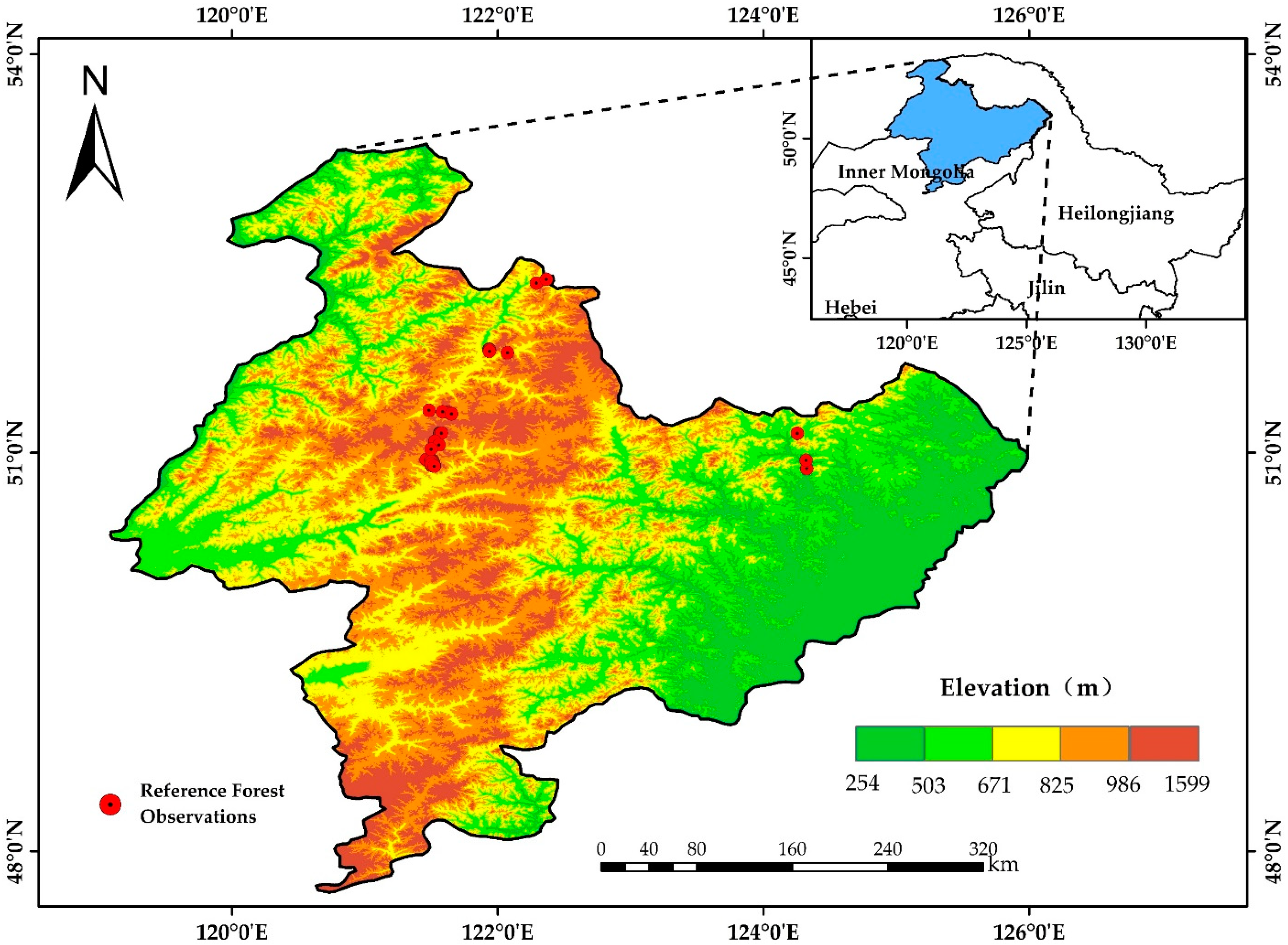
2.1. Study Area
2.2. Data and Preprocessing
2.2.1. Meteorological Data and Dendrochronological Measurements
2.2.2. Remote Sensing Data
2.3. Methods
2.3.1. The MOD_17 Model
2.3.2. Biome-BGCMuSo Model
2.3.3. Sensitivity Analysis
2.3.4. Incorporation of the MOD_17 and Biome-BGCMuSo
3. Results
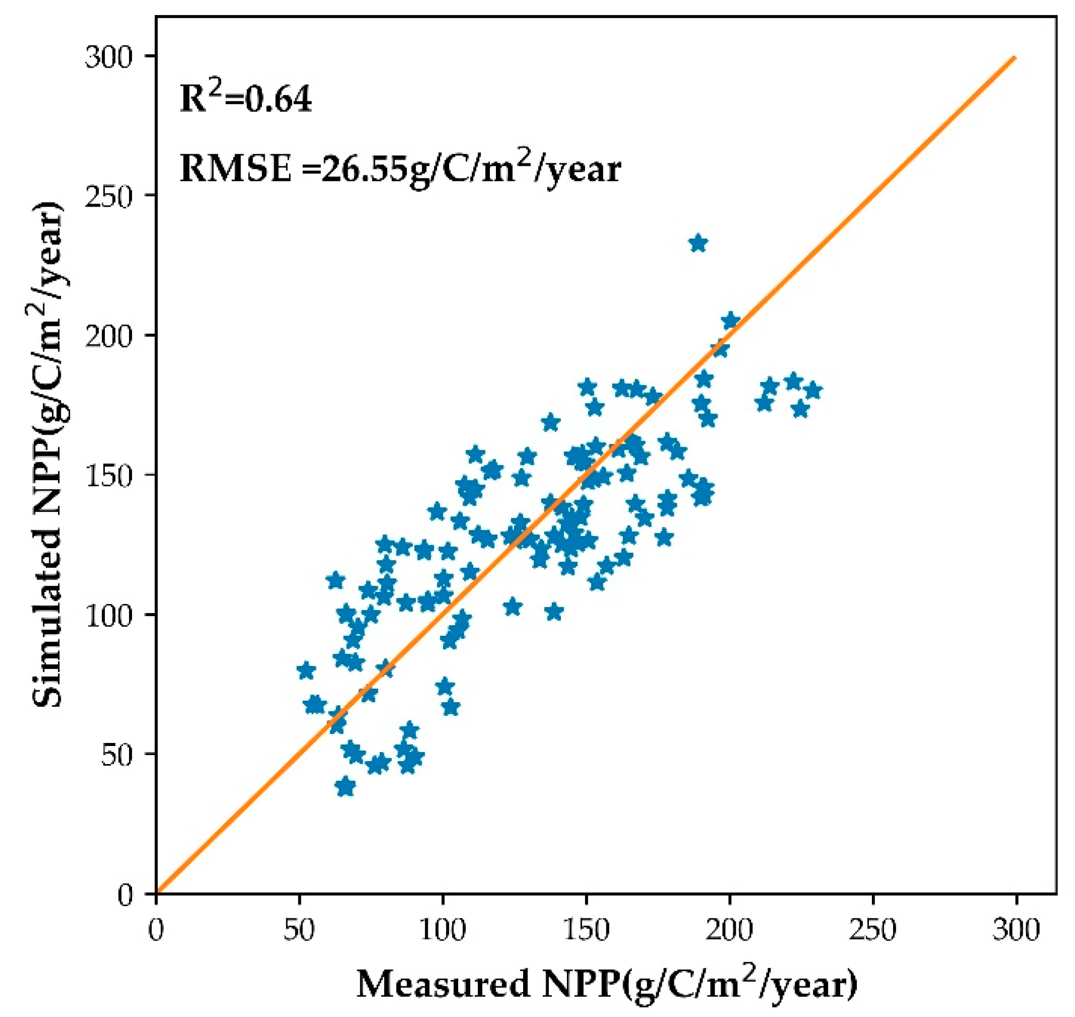
3.1. Optimization of the MOD_17 Model
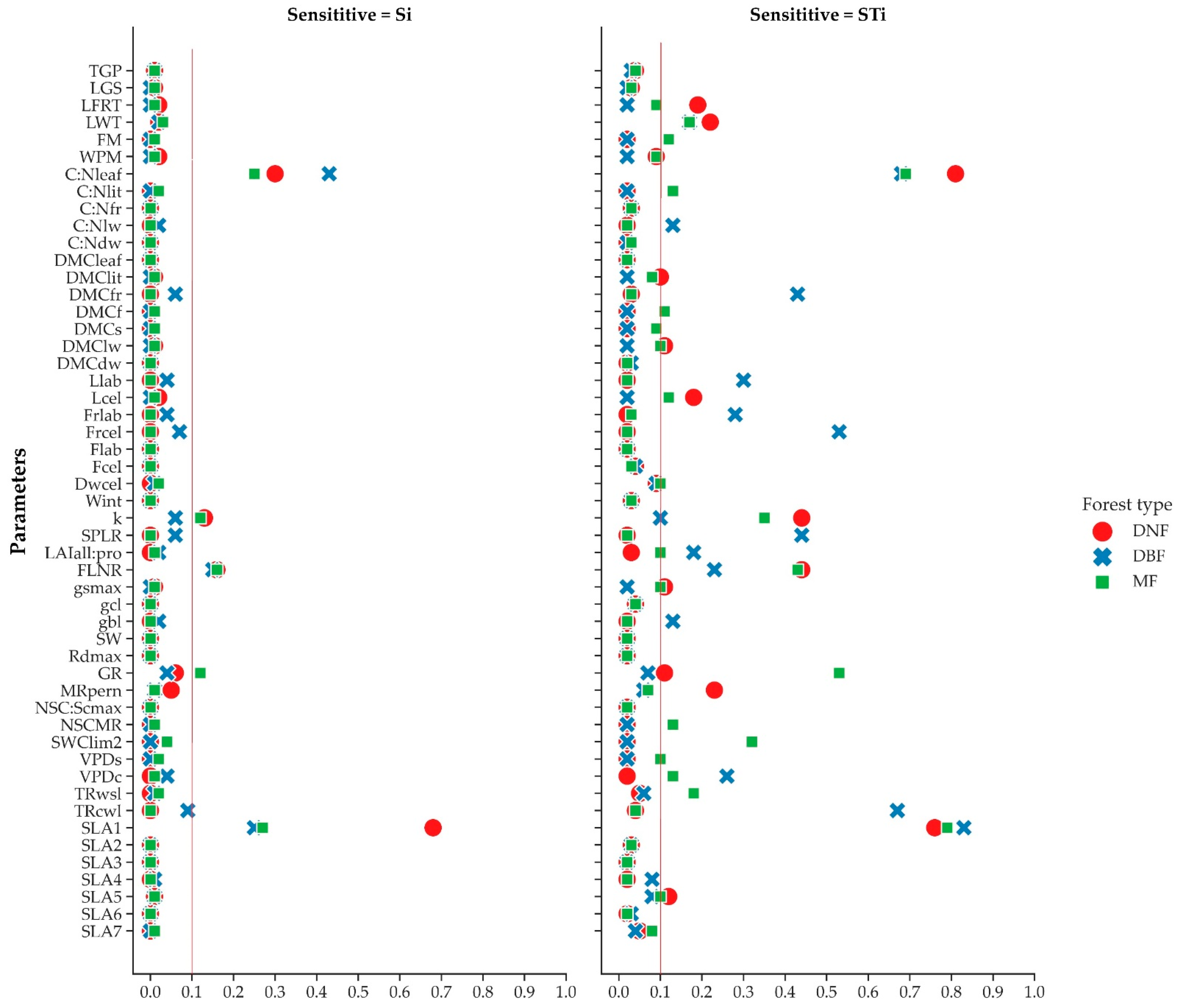
3.2. Sensitivity Analysis of Biome-BGCMuSo
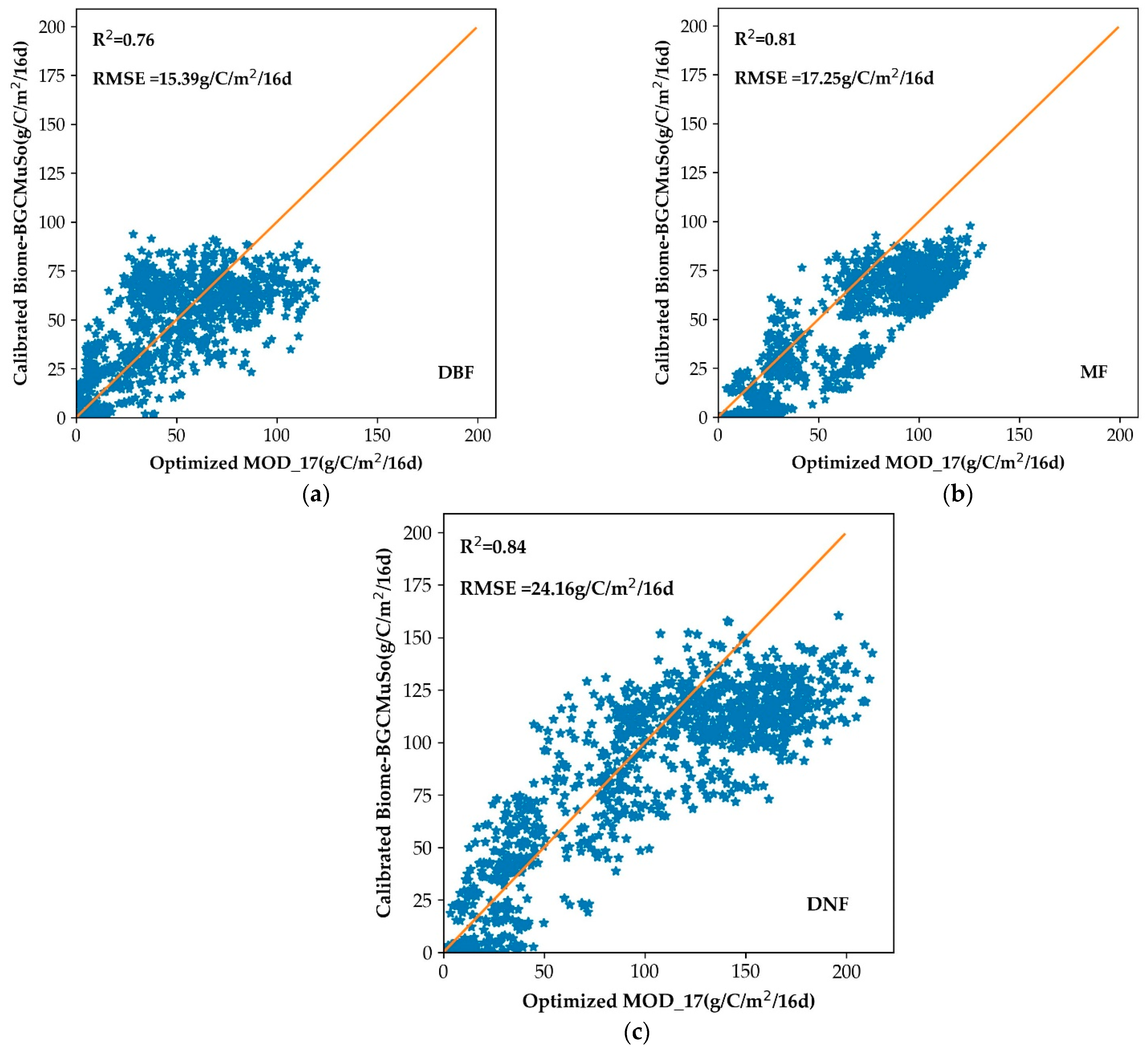
3.3. Calibration of Biome-BGCMuSo Mode
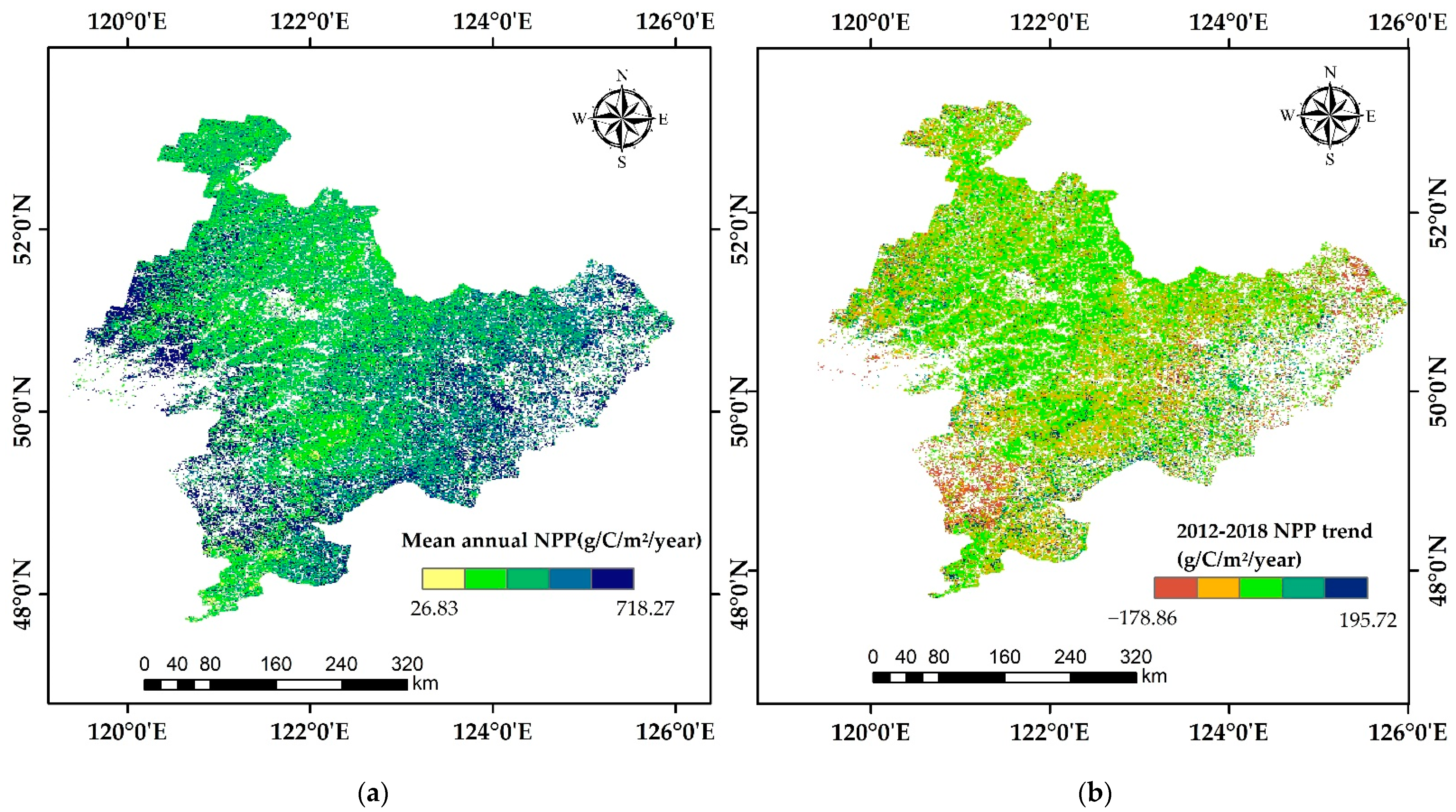
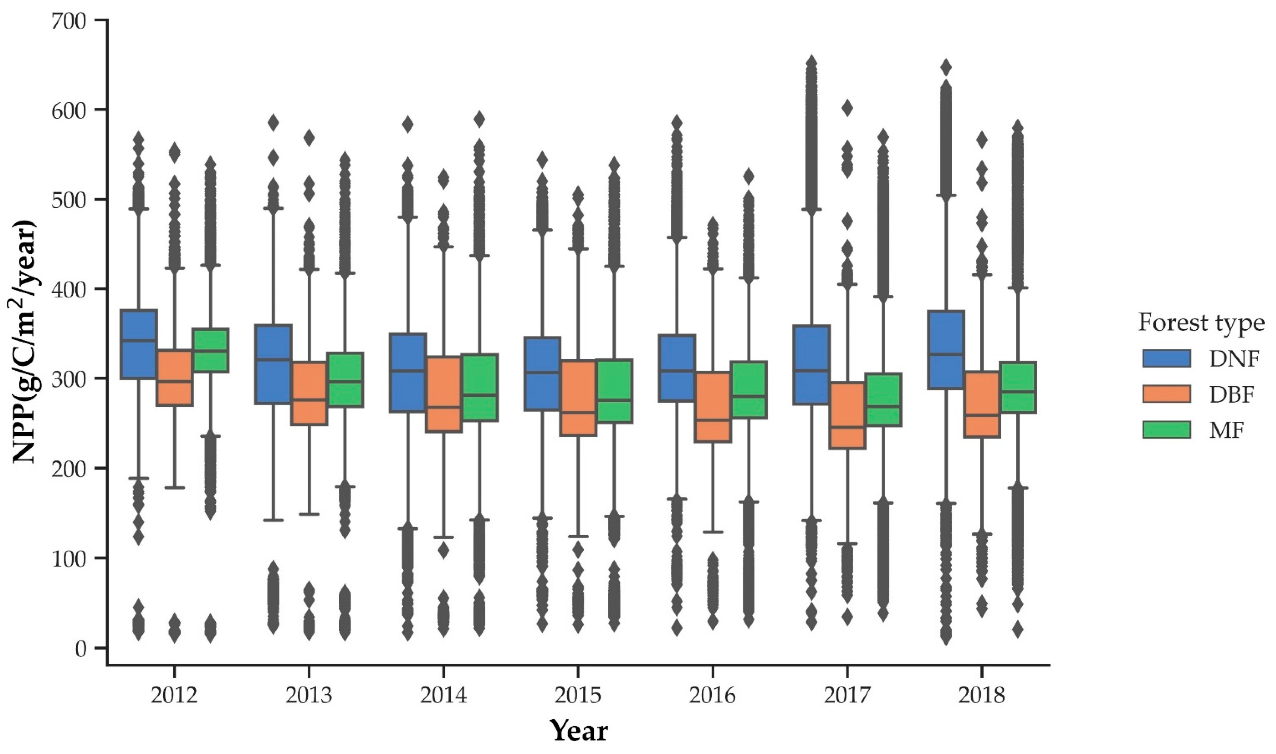
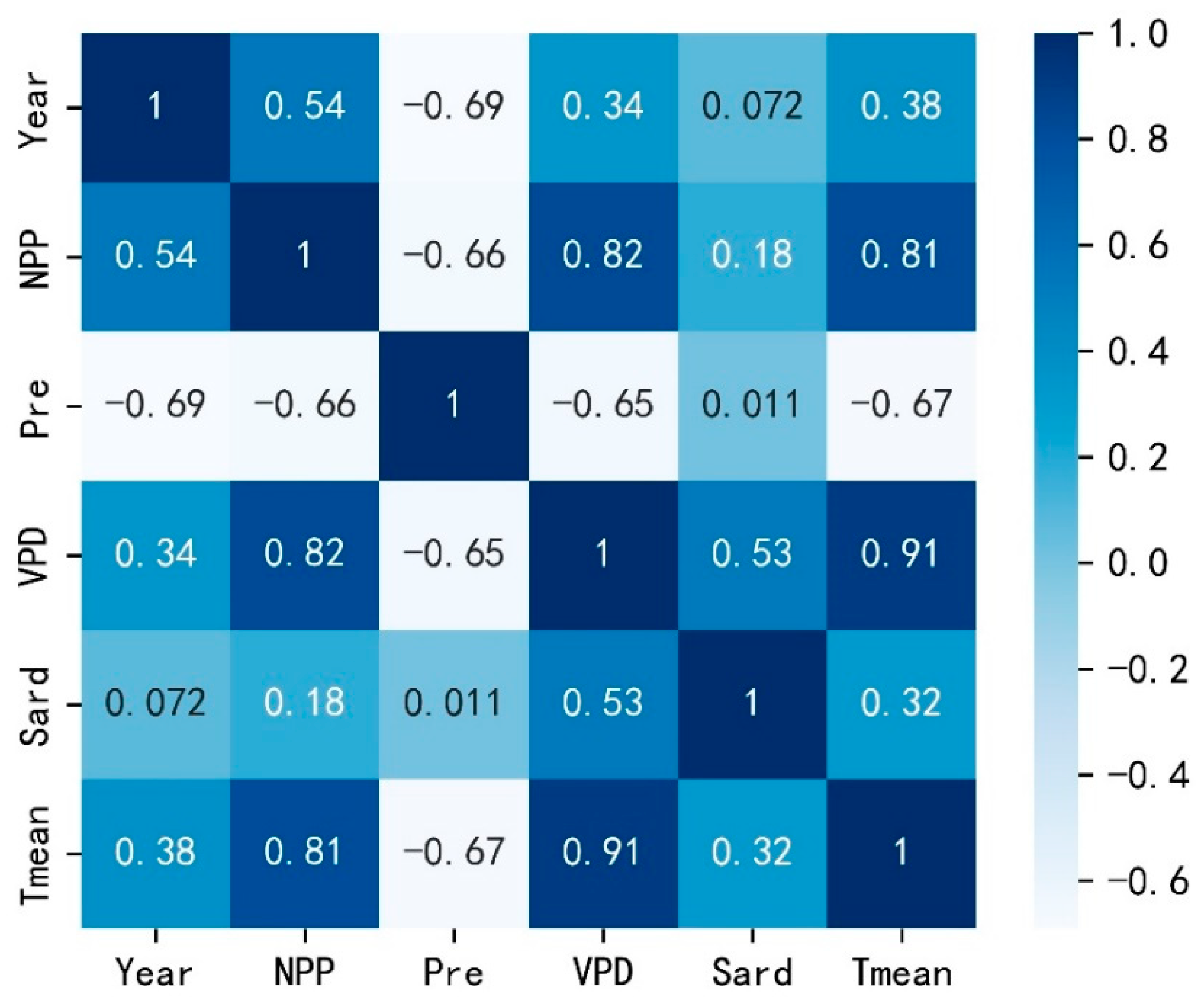
3.4. The Spatial and Temporal Dynamics Analysis of Forest NPP
4. Discussion
5. Conclusions
Supplementary Materials
Author Contributions
Funding
Data Availability Statement
Acknowledgments
Conflicts of Interest
References
- Pan, Y.; Birdsey, R.A.; Fang, J.; Houghton, R.; Kauppi, P.E.; Kurz, W.A.; Phillips, O.L.; Shvidenko, A.; Lewis, S.L.; Canadell, J.G.; et al. A large and persistent carbon sink in the world’s forests. Science 2011, 333, 988–993. [Google Scholar] [CrossRef] [PubMed]
- Tang, S.; Wang, X.; He, M.; Huang, L.; Zhang, Y.; Yang, H.; Piao, S. Global Patterns and Climate Controls of Terrestrial Ecosystem Light Use Efficiency. J. Geophys. Res. Biogeosciences 2020, 125, e2020JG005908. [Google Scholar] [CrossRef]
- Zhao, J.; Liu, D.; Cao, Y.; Zhang, L.; Peng, H.; Wang, K.; Xie, H.; Wang, C. An integrated remote sensing and model approach for assessing forest carbon fluxes in China. Sci. Total Environ. 2022, 811, 152480. [Google Scholar] [CrossRef]
- Gray, A.N.; Whittier, T.R. Carbon stocks and changes on Pacific Northwest national forests and the role of disturbance, management, and growth. For. Ecol. Manag. 2014, 328, 167–178. [Google Scholar] [CrossRef]
- Sinha, S.K.; Padalia, H.; Patel, N.R.; Chauhan, P. Modelling sun-induced fluorescence for improved evaluation of forest carbon flux (GPP): Case study of tropical deciduous forest, India. Ecol. Model. 2021, 449, 109552. [Google Scholar] [CrossRef]
- Cook-Patton, S.C.; Leavitt, S.M.; Gibbs, D.; Harris, N.L.; Lister, K.; Anderson-Teixeira, K.J.; Briggs, R.D.; Chazdon, R.L.; Crowther, T.W.; Ellis, P.W.; et al. Mapping carbon accumulation potential from global natural forest regrowth. Nature 2020, 585, 545–550. [Google Scholar] [CrossRef] [PubMed]
- Zhou, T.; Shi, P.; Jia, G.; Luo, Y. Nonsteady state carbon sequestration in forest ecosystems of China estimated by data assimilation. J. Geophys. Res. Biogeosciences 2013, 118, 1369–1384. [Google Scholar] [CrossRef]
- Zhao, J.; Xie, H.; Ma, J.; Wang, K. Integrated remote sensing and model approach for impact assessment of future climate change on the carbon budget of global forest ecosystems. Glob. Planet. Chang. 2021, 203, 103542. [Google Scholar] [CrossRef]
- Kang, F.; Li, X.; Du, H.; Mao, F.; Zhou, G.; Xu, Y.; Huang, Z.; Ji, J.; Wang, J. Spatiotemporal Evolution of the Carbon Fluxes from Bamboo Forests and their Response to Climate Change Based on a BEPS Model in China. Remote Sens. 2022, 14, 366. [Google Scholar] [CrossRef]
- Zhang, H.; Tang, S.; Wang, F. Study on establish and estimate method of biomass model compatible with volume. For. Res. 1999, 12, 53–59. [Google Scholar] [CrossRef]
- Ciais, P.; Reichstein, M.; Viovy, N.; Granier, A.; Ogée, J.; Allard, V.; Aubinet, M.; Buchmann, N.; Bernhofer, C.; Carrara, A. Europe-wide reduction in primary productivity caused by the heat and drought in 2003. Nature 2005, 437, 529–533. [Google Scholar] [CrossRef] [PubMed]
- Kljun, N.; Black, T.A.; Griffis, T.J.; Barr, A.G.; Gaumont-Guay, D.; Morgenstern, K.; McCaughey, J.H.; Nesic, Z. Response of net ecosystem productivity of three boreal forest stands to drought. Ecosystems 2007, 10, 1039–1055. [Google Scholar] [CrossRef]
- Chirici, G.; Chiesi, M.; Corona, P.; Salvati, R.; Papale, D.; Fibbi, L.; Sirca, C.; Spano, D.; Duce, P.; Marras, S.; et al. Estimating daily forest carbon fluxes using a combination of ground and remotely sensed data. J. Geophys. Res. Biogeosciences 2016, 121, 266–279. [Google Scholar] [CrossRef]
- Wen, J.; You, D.; Han, Y.; Lin, X.; Wu, S.; Tang, Y.; Xiao, Q.; Liu, Q. Estimating Surface BRDF/Albedo Over Rugged Terrain Using an Extended Multisensor Combined BRDF Inversion (EMCBI) Model. IEEE Geosci. Remote Sens. Lett. 2022, 19, 1–5. [Google Scholar] [CrossRef]
- Potter, C.S.; Randerson, J.T.; Field, C.B.; Matson, P.A.; Vitousek, P.M.; Mooney, H.A.; Klooster, S.A. Terrestrial ecosystem production: A process model based on global satellite and surface data. Glob. Biogeochem. Cycles 1993, 7, 811–841. [Google Scholar] [CrossRef]
- Prince, S.D.; Goward, S.N. Global Primary Production: A Remote Sensing Approach. J. Biogeogr. 1995, 22, 815–835. [Google Scholar] [CrossRef]
- Running, S.W.; Nemani, R.; Glassy, J.M.; Thornton, P.E. MODIS Daily Photosynthesis (PSN) and Annual Net Primary Production (NPP) Product (MOD17) Algorithm Theoretical Basis Document. University of Montana, SCFAt-Launch Algorithm ATBD Documents. Available online: www.ntsg.umt.edu/files/modis/ATBD_MOD17_v21.pdf (accessed on 16 October 2021).
- Veroustraete, F.; Sabbe, H.; Eerens, H. Estimation of carbon mass fluxes over Europe using the C-Fix model and Euroflux data. Remote Sens. Environ. 2002, 83, 376–399. [Google Scholar] [CrossRef]
- Running, S.W.; Hunt, E.R. Generalization of a Forest Ecosystem Process Model for Other Biomes, BIOME-BGC, and an Application for Global-Scale Models. In Scaling Physiological Processes; Ehleringer, J.R., Field, C.B., Eds.; Academic Press: San Diego, CA, USA, 1993; pp. 141–158. [Google Scholar] [CrossRef]
- Melillo, J.M.; McGuire, A.D.; Kicklighter, D.W.; Moore, B.; Vorosmarty, C.J.; Schloss, A.L. Global climate change and terrestrial net primary production. Nature 1993, 363, 234–240. [Google Scholar] [CrossRef]
- Liu, J.; Chen, J.M.; Park, W.M. A process-based boreal ecosystem productivity simulator using remote sensing inputs. Remote Sens. Environ. 1997, 62, 158–175. [Google Scholar] [CrossRef]
- Thornton, P.E.; Law, B.E.; Gholz, H.L.; Clark, K.L.; Falge, E.; Ellsworth, D.S.; Goldstein, A.H.; Monson, R.K.; Hollinger, D.; Falk, M. Modeling and measuring the effects of disturbance history and climate on carbon and water budgets in evergreen needleleaf forests. Agric. For. Meteorol. 2002, 113, 185–222. [Google Scholar] [CrossRef]
- Chiesi, M.; Maselli, F.; Moriondo, M.; Fibbi, L.; Bindi, M.; Running, S.W. Application of Biome-BGC to simulate Mediterranean forest processes. Ecol. Model. 2007, 206, 179–190. [Google Scholar] [CrossRef]
- Yan, M.; Tian, X.; Li, Z.; Chen, E.; Wang, X.; Han, Z.; Sun, H. Simulation of Forest Carbon Fluxes Using Model Incorporation and Data Assimilation. Remote Sens. 2016, 8, 567. [Google Scholar] [CrossRef]
- Tian, X.; Yan, M.; van der Tol, C.; Li, Z.; Su, Z.; Chen, E.; Li, X.; Li, L.; Wang, X.; Pan, X.; et al. Modeling forest above-ground biomass dynamics using multi-source data and incorporated models: A case study over the qilian mountains. Agric. For. Meteorol. 2017, 246, 1–14. [Google Scholar] [CrossRef]
- Yan, M.; Tian, X.; Li, Z.; Chen, E.; Li, C.; Fan, W. A long-term simulation of forest carbon fluxes over the Qilian Mountains. Int. J. Appl. Earth Obs. Geoinf. 2016, 52, 515–526. [Google Scholar] [CrossRef]
- Sánchez-Ruiz, S.; Maselli, F.; Chiesi, M.; Fibbi, L.; Martínez, B.; Campos-Taberner, M.; García-Haro, F.J.; Gilabert, M.A. Remote Sensing and Bio-Geochemical Modeling of Forest Carbon Storage in Spain. Remote Sens. 2020, 12, 1356. [Google Scholar] [CrossRef]
- Zhang, X.; Zhang, Q.; Sun, S.; Xu, Z.; Jian, Y.; Yang, Y.; Tian, Y.; Sa, R.; Wang, B.; Wang, F. Carbon exchange characteristics and their environmental effects in the northern forest ecosystem of the Greater Khingan Mountains in China. Sci. Total Environ. 2022, 838, 156056. [Google Scholar] [CrossRef]
- Yang, K.; He, J. China Meteorological Forcing Dataset (1979–2018); National Tibetan Plateau Data Center, Ed.; National Tibetan Plateau Data Center: Beijing, China, 2019. [Google Scholar] [CrossRef]
- He, J.; Yang, K.; Tang, W.; Lu, H.; Qin, J.; Chen, Y.; Li, X. The first high-resolution meteorological forcing dataset for land process studies over China. Sci. Data 2020, 7, 25. [Google Scholar] [CrossRef]
- Yang, K.; He, J.; Tang, W.; Qin, J.; Cheng, C.C.K. On downward shortwave and longwave radiations over high altitude regions: Observation and modeling in the Tibetan Plateau. Agric. For. Meteorol. 2010, 150, 38–46. [Google Scholar] [CrossRef]
- Dong, L.; Li, F.; Jia, W.; Liu, F.; Wang, H. Compatible biomass models for main tree species with measurement error in Heilongjiang Province of Northeast China. Chin. J. Appl. Ecol. 2011, 22, 2653–2661. [Google Scholar] [CrossRef]
- Wu, G.; Feng, Z. Study on the biomass of larix spp. forest community in the frigid-temperate zone and the temperate zone of China. J. Northeast For. Univ. 1995, 23, 95–101. [Google Scholar] [CrossRef]
- Li, H.; Lei, Y. Estimation and Evaluation of Forest Biomass Carbon Storage in China; China Forestry Publishing House: Beijing, China, 2010. [Google Scholar]
- Xiao, Z.; Liang, S.; Wang, J.; Chen, P.; Yin, X.; Zhang, L.; Song, J. Use of general regression neural networks for generating the GLASS leaf area index product from time-series MODIS surface reflectance. IEEE Trans. Geosci. Remote Sens. 2014, 52, 209–223. [Google Scholar] [CrossRef]
- Running, S.W.; Thornton, P.E.; Nemani, R.; Glassy, J.M. Global terrestrial gross and net primary productivity from the earth observing system. In Methods in Ecosystem Science; Sala, O.E., Jackson, R.B., Mooney, H.A., Howarth, R.W., Eds.; Springer: New York, NY, USA, 2000. [Google Scholar] [CrossRef]
- Monteith, J.L. Solar radiation and productivity in tropical ecosystems. J. Appl. Ecol. 1972, 9, 747–766. [Google Scholar] [CrossRef]
- Hidy, D.; Barcza, Z.; Hollós, R.; Thornton, P.E.; Running, S.W.; Fodor, N. User’s Guide for Biome-BGCMuSo 6.2. Available online: https://nimbus.elte.hu/bbgc/files/Manual_BBGC_MuSo_v6.2.pdf (accessed on 17 November 2021).
- Farquhar, G.D.; von Caemmerer, S.; Berry, J.A. A biochemical model of photosynthetic CO2 assimilation in leaves of C 3 species. Planta 1980, 149, 78–90. [Google Scholar] [CrossRef] [PubMed]
- Hidy, D.; Barcza, Z.; Marjanović, H.; Ostrogović Sever, M.Z.; Dobor, L.; Gelybó, G.; Fodor, N.; Pintér, K.; Churkina, G.; Running, S.; et al. Terrestrial ecosystem process model Biome-BGCMuSo v4.0: Summary of improvements and new modeling possibilities. Geosci. Model Dev. 2016, 9, 4405–4437. [Google Scholar] [CrossRef]
- Saltelli, A.; Tarantola, S.; Chan, K.P.S. A Quantitative Model-Independent Method for Global Sensitivity Analysis of Model Output. Technometrics 1999, 41, 39–56. [Google Scholar] [CrossRef]
- Campolongo, F.; Saltelli, A.; Tarantola, S. Sensitivity Anaysis as an Ingredient of Modeling. Stat. Sci. 2000, 15, 377–395. [Google Scholar] [CrossRef]
- White, M.A.; Thornton, P.E.; Running, S.W.; Nemani, R.R. Parameterization and sensitivity analysis of the Biome–BGC terrestrial ecosystem model: Net primary production controls. Earth Interact. 2000, 4, 1–85. [Google Scholar] [CrossRef]
- Huang, X.; Xiao, J.; Wang, X.; Ma, M. Improving the global MODIS GPP model by optimizing parameters with FLUXNET data. Agric. For. Meteorol. 2021, 300, 108314. [Google Scholar] [CrossRef]
- Li, X.; Liang, H.; Cheng, W. Evaluation and comparison of light use efficiency models for their sensitivity to the diffuse PAR fraction and aerosol loading in China. Int. J. Appl. Earth Obs. Geoinf. 2021, 95, 102269. [Google Scholar] [CrossRef]
- Ren, H.; Zhang, L.; Yan, M.; Tian, X.; Zheng, X. Sensitivity analysis of Biome-BGCMuSo for gross and net primary productivity of typical forests in China. For. Ecosyst. 2022, 9, 100011. [Google Scholar] [CrossRef]
- Houborg, R.; Cescatti, A.; Migliavacca, M. Constraining model simulations of GPP using satellite retrieved leaf chlorophyll. In Proceedings of the Geoscience and Remote Sensing Symposium (IGARSS), 2012 IEEE International, Munich, Germany, 22–27 July 2012. [Google Scholar]
- Li, X.H.; Sun, J.X. Testing parameter sensitivities and uncertainty analysis of Biome-BGC model in simulating carbon and water fluxes in broadleaved-korean pine forests. Chin. J. Plant Ecol. 2018, 42, 1131–1144. [Google Scholar] [CrossRef]
- Li, X.; Ma, H.; Ran, Y.; Wang, X.; Zhu, G.; Liu, F.; He, H.; Zhang, Z.; Huang, C. Terrestrial carbon cycle model-data fusion: Progress and challenges. Sci. Sin. Terrae 2021, 64, 1650–1663. [Google Scholar] [CrossRef]
- Xu, Y.; Xiao, F.; Yu, L. Review of spatio-temporal distribution of net primary productivity in forest ecosystem and its responses to climate change in China. Acta Ecol. Sin. 2020, 40, 4710–4723. [Google Scholar] [CrossRef]
- He, L.; Wan, H.; Wang, L.; Wang, Y. Response of net primary productivity of Larix olgensis forest ecosystem to climate change. J. Beijing For. Univ. 2015, 37, 28–36. [Google Scholar] [CrossRef]
- Li, Y.; Wang, Y.; Sun, Y.J.; Lei, Y.C.; Shao, W.C.; Li, J. Temporal-spatial characteristics of NPP and its response to climate change of Larix forests in Jilin Province. Acta Ecol. Sin. 2022, 42, 947–959. [Google Scholar] [CrossRef]


| Number | Parameter | Description | Unit |
|---|---|---|---|
| 1 | TGP | transfer growth period as fraction of growing season | prop. |
| 2 | LGS | litterfall as fraction of growing season | prop. |
| 3 | LFRT | annual leaf and fine root turnover fraction | 1/yr |
| 4 | LWT | annual live wood turnover fraction | 1/yr |
| 5 | FM | annual fire mortality fraction | 1/yr |
| 6 | WPM | whole-plant mortality fraction in vegetation period | 1/yr |
| 7 | C:Nleaf | C:N of leaves | kgC/kg N |
| 8 | C:Nlit | C:N of leaf litter, after retranslocation | kgC/kg N |
| 9 | C:Nfr | C:N of fine roots | kgC/kg N |
| 10 | C:Nlw | C:N of live wood | kgC/kg N |
| 11 | C:Ndw | C:N of dead wood | kgC/kg N |
| 12 | DMCleaf | dry matter carbon content of leaves | (kgC/kgDM) |
| 13 | DMClit | dry matter carbon content of leaf litter | (kgC/kgDM) |
| 14 | DMCfr | dry matter carbon content of fine roots | (kgC/kgDM) |
| 15 | DMCf | dry matter carbon content of fruit | (kgC/kgDM) |
| 16 | DMCs | dry matter carbon content of soft stem | (kgC/kgDM) |
| 17 | DMClw | dry matter carbon content of live wood | (kgC/kgDM) |
| 18 | DMCdw | dry matter carbon content of dead wood | (kgC/kgDM) |
| 19 | Llab | leaf litter labile proportion | DIM |
| 20 | Lcel | leaf litter cellulose proportion | DIM |
| 21 | FRlab | P fine root labile proportion | DIM |
| 22 | FRcel | fine root cellulose proportion | DIM |
| 23 | Flab | fruit litter labile proportion | DIM |
| 24 | Fcel | fruit litter cellulose proportion | DIM |
| 25 | DWcel | dead wood cellulose proportion | DIM |
| 26 | Wint | canopy water interception coefficient | 1/LAI/d |
| 27 | k | canopy light extinction coefficient | DIM |
| 28 | SPLR | all-sided to projected leaf area ratio | DIM |
| 29 | LAIall:pro | ratio of shaded SLA:sunlit SLA | DIM |
| 30 | FLNR | fraction of leaf N in Rubisco | DIM |
| 31 | gsmax | maximum stomatal conductance (projected area basis) | m/s |
| 32 | gcl | conductance (projected area basis) | m/s |
| 33 | gbl | boundary layer conductance (projected area basis) | m/s |
| 34 | SW | stem weight corresponding to maximum height | (kgC) |
| 35 | Rdmax | maximum depth of rooting zone | (m) |
| 36 | GR | growth resp per unit of C grown | (prop.) |
| 37 | MRpern | maintenance respiration in kg C/day per kg of tissue N | (kgC/kgN/d) |
| 38 | NSC:Scmax | theoretical maximum prop. of non-structural and structural carbohydrates | (DIM) |
| 39 | NSCMR | of non-structural carbohydrates available for maintenance respiration | (DIM) |
| 40 | SWClim2 | minimum of soil moisture limit2 multiplicator (full anoxic stress value) | prop |
| 41 | VPDs | vapor pressure deficit: start of conductance reduction | Pa |
| 42 | VPDc | vapor pressure deficit: complete conductance reduction | Pa |
| 43 | TRwsl | turnover rate of wilted standing biomass to litter | prop |
| 44 | TRcwl | turnover rate of non-woody cut-down biomass to litter | prop |
| 45 | SLA1 | canopy average specific leaf area in phenological phase 1 | m2/kg |
| 46 | SLA2 | canopy average specific leaf area in phenological phase 2 | m2/kg |
| 47 | SLA3 | canopy average specific leaf area in phenological phase 3 | m2/kg |
| 48 | SLA4 | canopy average specific leaf area in phenological phase 4 | m2/kg |
| 49 | SLA5 | canopy average specific leaf area in phenological phase 5 | m2/kg |
| 50 | SLA6 | canopy average specific leaf area in phenological phase 6 | m2/kg |
| 51 | SLA7 | canopy average specific leaf area in phenological phase 7 | m2/kg |
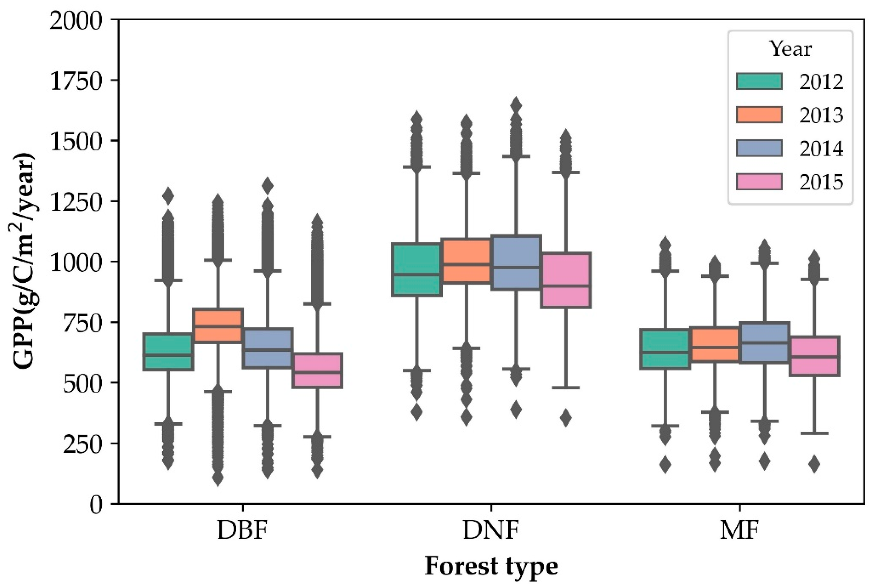
| Year | Forest Type | Count | Mean | STD | Min | Max | CV (%) |
|---|---|---|---|---|---|---|---|
| 2012 | DBF | 41,583 | 635.48 | 130.39 | 176.43 | 1269.95 | 20.52 |
| DNF | 7651 | 977.62 | 160.46 | 378.92 | 1585.82 | 16.41 | |
| MF | 22,631 | 641.17 | 114.07 | 160.94 | 1067.52 | 17.79 | |
| 2013 | DBF | 41,580 | 737.82 | 118.83 | 108.4 | 1242.4 | 16.1 |
| DNF | 7651 | 1008.21 | 144.6 | 357.08 | 1571.69 | 14.34 | |
| MF | 22,630 | 657.27 | 102.53 | 167.75 | 989.16 | 15.6 | |
| 2014 | DBF | 41,575 | 646.63 | 139.75 | 138.71 | 1312.03 | 21.61 |
| DNF | 7650 | 1000.89 | 158.98 | 388.92 | 1643.15 | 15.88 | |
| MF | 22,628 | 665.82 | 114.89 | 175.5 | 1055.16 | 17.25 | |
| 2015 | DBF | 41,578 | 561.34 | 125.7 | 139.76 | 1160.08 | 22.39 |
| DNF | 7649 | 927.53 | 157.95 | 353.94 | 1509.93 | 17.03 | |
| MF | 22,628 | 611.4 | 110.91 | 163.67 | 1012.6 | 18.14 |
Publisher’s Note: MDPI stays neutral with regard to jurisdictional claims in published maps and institutional affiliations. |
© 2022 by the authors. Licensee MDPI, Basel, Switzerland. This article is an open access article distributed under the terms and conditions of the Creative Commons Attribution (CC BY) license (https://creativecommons.org/licenses/by/4.0/).
Share and Cite
Su, Y.; Zhang, W.; Liu, B.; Tian, X.; Chen, S.; Wang, H.; Mao, Y. Forest Carbon Flux Simulation Using Multi-Source Data and Incorporation of Remotely Sensed Model with Process-Based Model. Remote Sens. 2022, 14, 4766. https://0-doi-org.brum.beds.ac.uk/10.3390/rs14194766
Su Y, Zhang W, Liu B, Tian X, Chen S, Wang H, Mao Y. Forest Carbon Flux Simulation Using Multi-Source Data and Incorporation of Remotely Sensed Model with Process-Based Model. Remote Sensing. 2022; 14(19):4766. https://0-doi-org.brum.beds.ac.uk/10.3390/rs14194766
Chicago/Turabian StyleSu, Yong, Wangfei Zhang, Bingjie Liu, Xin Tian, Shuxin Chen, Haiyi Wang, and Yingwu Mao. 2022. "Forest Carbon Flux Simulation Using Multi-Source Data and Incorporation of Remotely Sensed Model with Process-Based Model" Remote Sensing 14, no. 19: 4766. https://0-doi-org.brum.beds.ac.uk/10.3390/rs14194766