
Geomorphic Evolution of Radial Sand Ridges in the South Yellow Sea Observed from Satellites


1
Key Laboratory of Marine Hazards Forecasting, Ministry of Natural Resources, Hohai University, Nanjing 210024, China
2
College of Oceanography, Hohai University, Nanjing 210024, China
3
College of Hydrology and Water Resources, Hohai University, Nanjing 210024, China
*
Author to whom correspondence should be addressed.
Remote Sens. 2022, 14(2), 287; https://0-doi-org.brum.beds.ac.uk/10.3390/rs14020287
Submission received: 25 November 2021
/
Revised: 1 January 2022
/
Accepted: 4 January 2022
/
Published: 9 January 2022
(This article belongs to the Special Issue Remote Sensing Application in Coastal Geomorphology and Processes)
Abstract
:The radial sand ridges consist of more than 70 sand ridges that are spread out radially on the continental shelf of the South Yellow Sea. As a unique geomorphological feature in the world, its evolution process and characteristics are crucial to marine resource management and ecological protection. Based on the multi-source remote sensing image data from 1979 to 2019, three types of geomorphic feature lines, artificial coastlines, waterlines, and sand ridge lines were extracted. Using the GIS sequence analysis method (Digital Shoreline Analysis System (DSAS), spatial overlay analysis, standard deviational ellipse method), the evolution characteristics of the shoreline, exposed tidal flats, and underwater sand ridges from land to sea were interpreted. The results demonstrate that: (1) The coastline has been advancing towards the sea with a maximum advance rate of 348.76 m/a from Wanggang estuary to Xiaoyangkou Port. (2) The exposed tidal flats have decreased by 1484 km2 including the reclaimed area of 1414 km2 and showed a trend of erosion in the north around Xiyang channel and deposition in the southeast around the Gaoni and Jiangjiasha areas. (3) The overall sand ridge lines showed a trend of gradually moving southeast (135°), and the moving distance is nearly 4 km in the past 40 years. In particular, the sand ridge of Tiaozini has moved 11 km southward, while distances of 8 km for Liangyuesha and 5 km for Lengjiasha were also observed. For the first time, this study quantified the overall migration trend of the RSRs. The imbalance of the regional tidal wave system may be one of the main factors leading to the overall southeastward shift of the radiation sandbanks.
1. Introduction
The radial sand ridges (RSRs), which are located on the continental shelf of the South Yellow Sea, have outstanding geological value because of their unique radial landform structure and large area of tidal flats [1]. The two largest Chinese rivers, the Yangtze River and the Yellow River, have supplied huge quantities of sediment since early Cenozoic times [2]. Due to abundant sediment and nutrients, it is very suitable for the reproduction and habitat of wetland creatures, especially birds. As an irreplaceable fortress on the East Asia–Australian bird migration route, it is the core plate of the world’s natural heritage and China’s migratory bird sanctuaries along the coast of the Yellow Sea–Bohai Gulf (Phase I) [3]. In the past 40 years, the RSRs have withstood pressure from land and sea. On the one hand, land reclamation activities on the Jiangsu coast are very frequent and high intensity. From 2007 to 2014, the reclamation area steeply increased from 118 to 533 km2 in the onshore coast of radial sandbank [4]. On the other hand, the incoming sand from the Yangtze River in the south dropped sharply due to the Three Gorges Project [5], and the underwater delta of the abandoned Yellow River in the north was eroded out [6,7]. As a result, the source of sediment in the RSRs is insufficient and shows a rapid and active morphological change, and the erosion of the northern tidal flats, led by both sides of Xiyang tidal channel, is obvious [8]. Under the changing macroenvironment, what is the future trend of the RSRs? To solve this problem, we need to study the characteristics of changes in the past few decades. In addition, monitoring the geomorphological evolution of RSRs is therefore essential for local ecological protection, resource management, and coastal sustainable development.
A field survey based on ship-based echo sounding and real-time kinematic (RTK) is a traditional and direct method used to analyze the geomorphic evolution of the coast or sea floor [9]. Since the 1980s, several large-scale field surveys have been carried out, covering hydrology, coastal climate, geological history, sediment composition, suspended solids, and geomorphic characteristics [10,11,12]. Cross-sectional measurement is more common in the analysis of geomorphological changes. Wang et al. [13] recognized that the intertidal flat has become narrower and steeper, following sequential reclamations using seabed elevation data along profile and corresponding grain size parameter variations from May to December 2008. Based on 15 monthly field surveys along a transect from September 2012 to November 2013, Gong et al. [14] indicated that the cross-shore profile shows a clear double-convex shape. Field survey data are mostly analyzed from a local, short-term, and historical perspective, while the macro-integrated, long-term, and current observations are often limited by technology and natural environmental conditions [15]. In addition, numerical models are also used to simulate sediment transportation, and the dynamic mechanism is also discussed. Xu et al. [16] suggest that the northern and southern channel shoals may be treated as two relatively independent geomorphological systems characterized by different tidal flows and sediment compositions. Tao et al. [17] constructed an ideal morphological dynamics model of RSRs and predicted the geomorphological evolution trend over a long timescale. Zhang et al. [18] used a hydrodynamic model applied to an idealized fan-shaped basin to explore the morphology and dynamics of radial sand ridges in a convergent coastal system. Due to the limitations of grid resolution and measured seabed topography data, at present, the numerical model method mostly involves an ideal model and mechanism analysis [19].
Remote sensing combined with geographic information system (GIS) technology has been an effective method for studying the morpho-hydrodynamics of coastal areas [15,20,21]. Numerous satellite images with increasing spatial, temporal, and spectral resolution have been archived since the launch of the Landsat-1 satellite in 1972 [22]. Murray et al. [23] tracked losses of tidal wetlands in the Yellow Sea using Landsat images. Jia et al. [24] produced an up-to-date 10-m spatial resolution tidal flat map of China using time series Sentinel-2 images. The widely adopted waterline method—using a time series of satellite images to construct a digital elevation model (DEM) of tidal flats—is an established technique for the measurement of tidal flat topography from macro- to meso-scale [25,26,27,28]. Wang et al. [8] implemented three-dimensional terrain analysis to estimate the trend of tidal flat evolution of Jiangsu middle coast based on a time series of digital elevation models (DEMs). However, previous studies in Jiangsu coast have mostly focused on the evolution of exposed tidal flats but have lacked simultaneous analysis of the supra-tidal zone and the unexposed underwater sandbanks. The overall geomorphic evolution of the RSRs still needs further quantitative discussion and historical comparison.
From the perspective of geomorphology, the RSRs from land to sea can be divided into three parts: land bounded by artificial shoreline, exposed tidal flats bounded by waterline, and sand ridges submerged by sea water. The coastline, tidal flat waterline, and sand ridge line in all kinds of geomorphic units have clear recognition and representation. Therefore, in this study, we attempted to extract the shoreline, waterline, and sand ridge line using multi-source and multi-temporal remote sensing images from 1979 to 2019. With GIS technology, the spatial and temporal characteristics of shorelines, waterlines, and sand ridge lines in the past 40 years were quantitatively analyzed, revealing the overall geomorphic evolution characteristics of the RSRs.
2. Study Area
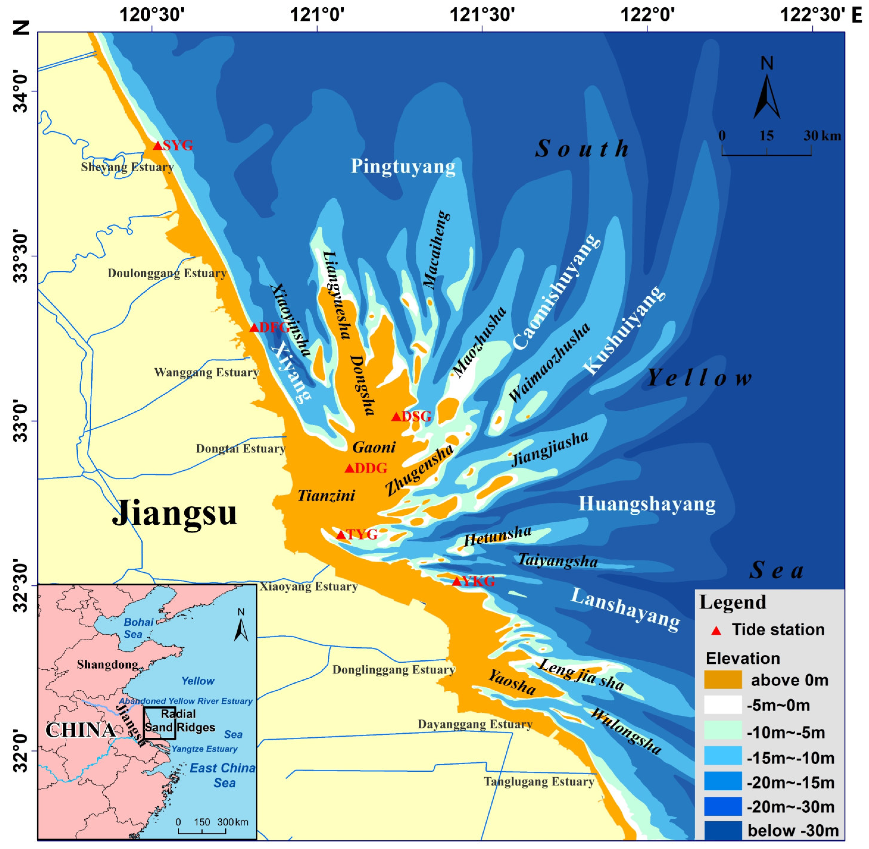
The RSRs bordered by the Old Yellow River mouth in the north and the Yangtze River estuary in the south located in the northern coast of Jiangsu province, China (Figure 1). From Sheyang estuary to Tanglugang estuary, it covers a sea area of more than 20,000 km2 with a length of about 200 km and a width of about 90 km. More than 70 sand ridges with various dimensions radiate from the Tiaozini towards the open sea. The water depth ranges from 0 to 30 m (theoretical depth base) [29]. The exposed tidal flats with an area of more than 2000 km2 are typically dozens of kilometers wide with an average slope of approximately 0.2% and an increase in slope to 1.5% near the tidal creeks [27]. The bottom sediment of the RSRs mainly consists of fine sand [30], with a mean grain size of 62.5–250 μm, and the sediment mixture is well-sorted [31].
The RSRs area is affected by two tidal wave systems. One is the advancing tide wave from the East China Sea, which enters the Yellow Sea from south to north. The other is the counterclockwise rotating tide wave, which is formed by the reflection of the East China Sea advancing tide through the Shandong Peninsula. The two tidal waves meet in the RSRs, where the crest lines of the two tidal waves meet, forming a ‘standing wave’ area in the fan-shaped area outside the Tiaozini [32]. Therefore, tidal ranges are normally 4–6 m but can reach up to 9.36 m in the Tiaoyugang south of Tiaozini [33].
3. Materials and Methods
3.1. Dataset
Considering the characteristics of the sea area and the research needs of the RSRs, remote sensing images need to be carefully selected. On the one hand, tidal conditions should be considered so that the water line extraction of exposed tidal flats can be carried out at a low tide condition. On the other hand, the boundary between sandbanks and tidal creeks should be obvious in the image to facilitate the extraction of sub-water sand ridges. Meanwhile, in order to facilitate the analysis of the long-term sequence of landform changes, we selected the optical multispectral image data from the 1970s to the present as the main data source, such as Landsat, HJ-1, and GF-1. (Table 1). With 1979, 1989, 1999, 2009, and 2019 as time nodes, remote sensing images for 1–2 years before and after the nodes were collected. The remote sensing images were preprocessed by band composition, strip-stripping, image enhancement processing, and geometric correction. A topographic map (1:50,000) of the Jiangsu coastal zone was used as the reference image for geometric correction. The correct accuracy was controlled within a pixel. All images were projected onto ‘WGS_1984_UTM_Zone_51N’ datum planes. The Chinese National Height Datum 1985 (CNHD 1985) was adopted for the five tide stations shown in Figure 1.
Tide gauge data were obtained from five tide level stations: Yangkougang, Tiaoyugang, Dongdagang, Dongshagang, and Dafenggang in the sea area of RSRs (Figure 1). Because the five tide level stations were built in 2012 [33], the historical data of each station is calculated by the harmonic analysis. The formula is as follows:
where is time; is the tide height; is the height of the annual or annual mean sea level; is the serial number of the tidal constituent; is the total number of tidal constituents; is the intersection factor of the tidal constituent; is the amplitude of the tidal constituent; is the tidal angular velocity; is the tidal phase angle; is the correction angle of fractional tide intersection; and is a special late angle for tidal separation.
3.2. Methods
3.2.1. Shoreline Extraction and Analysis
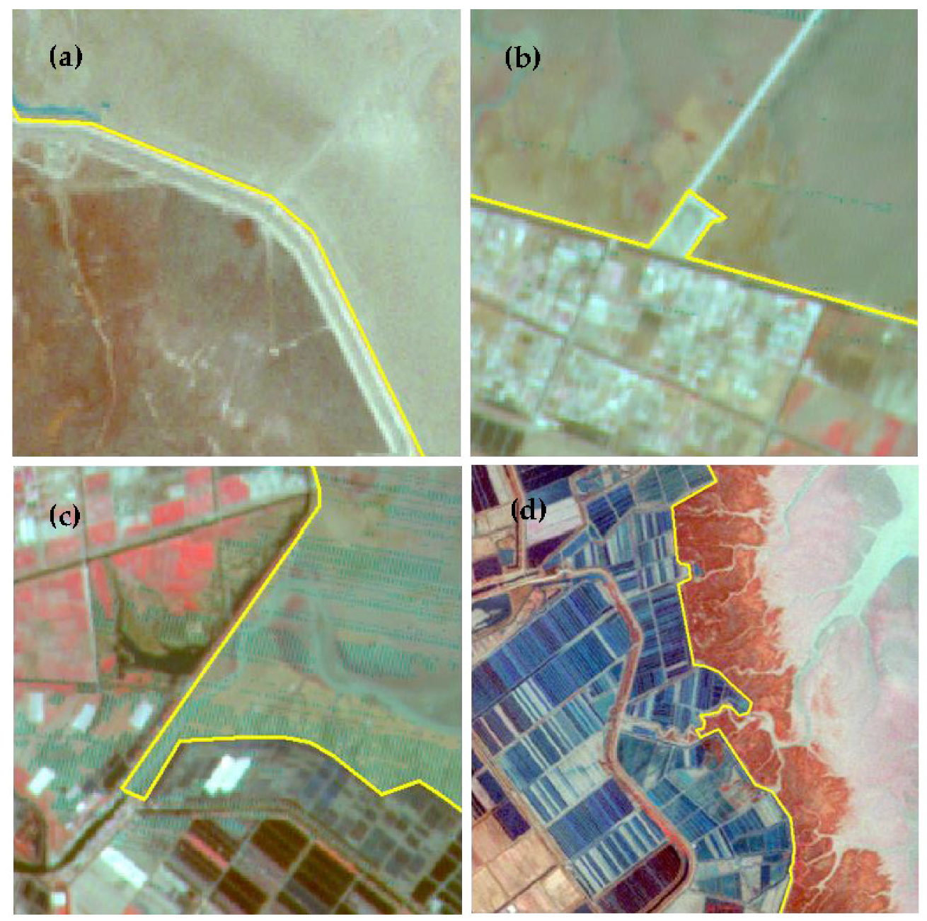
An artificial shoreline is a borderline formed by artificial buildings, including reclamation seawalls, wharves, fishponds, and salt pans. From the Sheyang to Tanglugang estuary, large-scale exposed tidal flats are an extremely active area for reclamation activities. In recent decades, more than 1000 km2 of tidal flats have been reclaimed. The shoreline has gradually advanced to the sea, and the natural shoreline has almost been replaced by artificial shoreline. The artificial shoreline is the edge line of the outermost artificial structures on the beach. Because of different uses, artificial structures include tidal dikes, breakwaters, ports, docks, protruding dikes, breeding ponds, and salt pans. They are generally straight and clear and not affected by the water level. These ‘standard false color composite images’ (R: near-infrared band; G: red band; B: green band)—such as Landsat MSS (654); Landsat TM/ETM+ (432); Landsat OLI (543); HJ−1 CCD (432); GF−1 WFV (432)—were used to extract historical artificial shorelines in RSRs area. As shown in Figure 2, artificial structures such as tide dikes or breakwaters are generally bright in the image, appearing white, with long and narrow extensions and smooth textures; outside the dikes are silt mud flats with dark colors. The position of the shoreline is the outer edge of the white border. For ports and docks, there are mostly residential areas or factories, etc., with uneven brightness and clear mesh textures, which are easy to confirm. The position of the coastline is determined at the line connecting the root of the protruding dike to the land. The breeding ponds are elongated and distributed more concentratedly. The color of the breeding ponds on the images is close to sea water, and looks gray or off-white when it dries up. For the estuary, the sharp narrowing of the channel at the small estuary and the maximum curvature of the two headlands are defined as the shoreline. Therefore, in this study, visual interpretation of remote sensing images was carried out to extract historical artificial shorelines in RSR areas.
Based on historical artificial shorelines, evolution analysis was executed using the Digital Shoreline Analysis System (DSAS) version 5.0 [34]. DSAS is a quantitative analysis system developed by The United States Geological Survey to calculate the temporal and spatial change rate of the shoreline that works within the Esri Geographic Information System (ArcGIS) software. The specific process is as follows: (1) Extraction of shorelines. All shoreline positions that are to be used in the change-rate analysis must reside in a single feature class in the geodatabase. (2) Baseline creation. Baselines are created using a buffer method with the same curved shape as the shoreline. (3) Generating transects. Set the spacing of crosscutting lines as 1 km, generating a total of 257 crosscutting lines that intersect all shorelines. (4) Selection of statistics to calculate. Shoreline change information can be calculated by DSAS, such as shoreline change envelope (SCE), net shoreline movement (NSM), linear regression rate (LRR), and end point rate (EPR). NSM is the distance between the oldest and youngest shorelines in a certain period, which can scientifically and effectively simulate the temporal and spatial change rate of the shoreline.
3.2.2. Waterline Extraction and Analysis
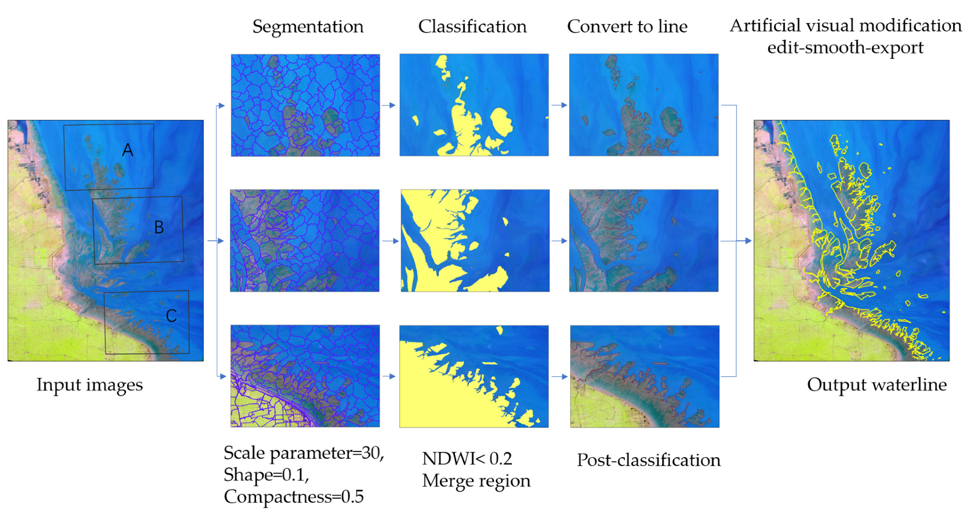
The ‘waterline’ is defined as the boundary between a water body and an exposed tidal flat in a remotely sensed image. The tidal flat was characterized by a low reflectance from the exposed surface, a high seawater turbidity, and a variation in moisture content that was in turn governed by grain size, local slope, and the existence of tidal channels or creeks [35]. Therefore, in different areas, different bands or spectral digital number values of remote sensing image should be determined to extract waterlines over the entire region [33]. In this study, a method based on object-oriented classification was used to extract waterlines. The object-oriented classification method makes use of the features of shape, texture, and landscape to realize high-precision classification results using the technologies of images segmentation, multiple feature analysis and extraction, sample selection, and supervised classification [36]. At the same time, object-oriented classification can establish different segmentation thresholds for different images and can directly obtain the vector surface of each object, so it can effectively avoid the problem of broken lines in the process of waterline extraction.
As shown in Table 1, multi-source images such as Landsat (MSS, TM, ETM+, OLI), HJ−1, GF−1 were used to extract the waterlines. The spatial resolution of MSS image is 79 m, TM, ETM+ 30 m, HJ−1 30 m, and GF−1 16 m. In addition, the ‘standard false color composite image’, that is, the near-infrared band corresponds to R (red), the red band corresponds to G (green), and the green band corresponds to B (blue) as the initial image to be processed. As shown in Figure 3, the steps of the extraction method mainly include image segmentation based on multi-scale, region merging, and artificial visual modification. eCognition software (version 9.1) was used to complete waterline extraction. Multi-scale segmentation is one of the most used segmentation algorithms, and the scale-level parameter in this study was set to 30. The normalized difference water index (NDWI) was used for region merging to combine small segments into groups. Finally, the waterlines were output and further modified manually. In order to study the overall movement trend and area change of the tidal flat, we converted the waterlines into polygons. Different polygon layers in one year before and after the time node (1979/1989/1999/2009/2019) were merged to obtain a maximum outsourcing polygon which was used as the exposed tidal flat layer at a specific time node in subsequent analysis. In addition, GIS spatial overlay analysis was implemented to analyze the area variation and spatial stability of exposed tidal flats from 1979 to 2019.
3.2.3. Sand Ridge Line Extraction and Analysis
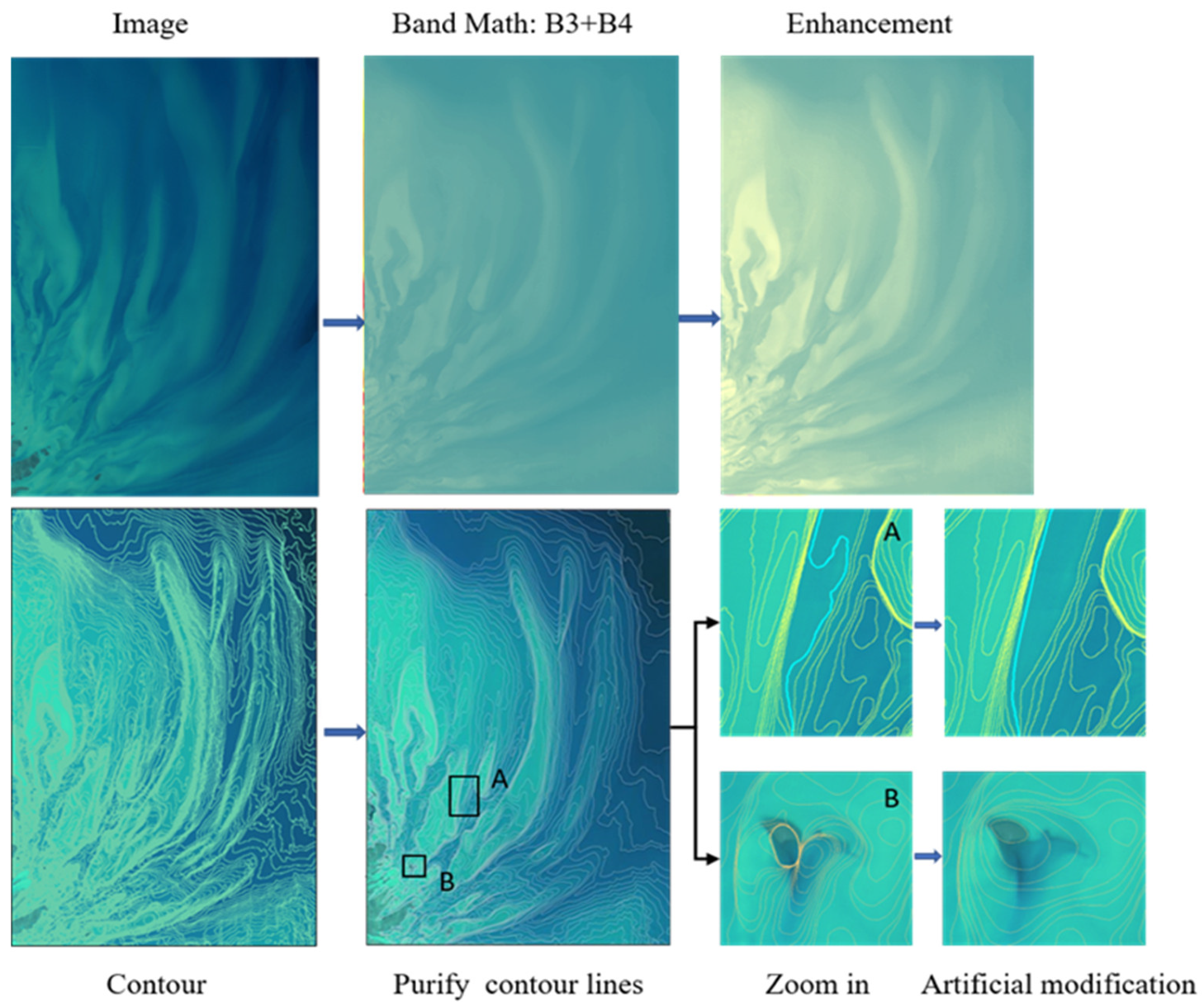
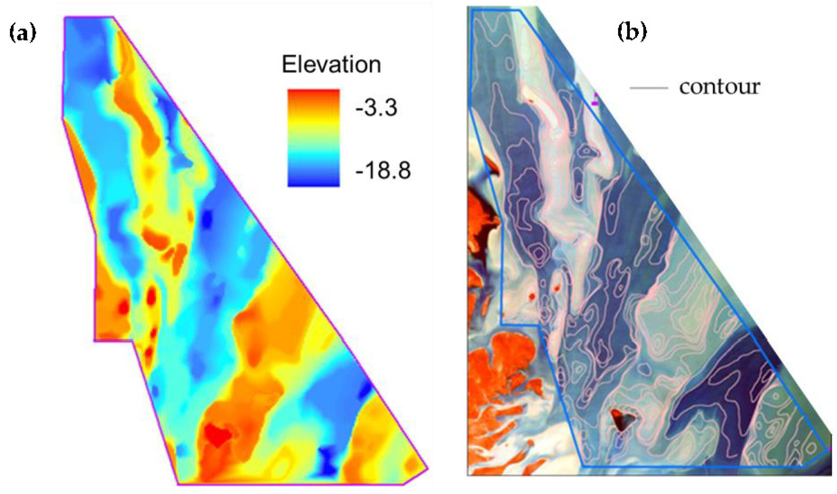
In this study, based on radiation contours, the sand ridge lines in the RSRs were extracted through visual interpretation. The extraction process is briefly described by taking the HJ−1 image on 26 April 2012 as an example (Figure 4). It mainly includes four steps: image selection, characteristic band (red band + near-infrared band: B3+B4 in HJ−1) determination, piecewise linear enhancement processing, and contour extraction. ① Image selection: Through the analysis of the tide situation corresponding to the historical satellite images, it was found that the image about 2 h after the lowest tide should be selected as the data source. After the ebb tide, flow velocity is small, and the sediment is not easily suspended. At this gap time, the concentration of suspended sediment is low, and the underwater sand ridges are clearly visible on the acquired remote sensing image. ② Characteristic band determination: A previous study made it apparent that the correlation coefficients between spectral band and total suspended matter (TSM) become larger as the wavelengths shift from the blue to the near-infrared bands [37]. In this study, the correlation between the measured topographic data and various band combinations was analyzed. It was found that the ‘red band + near-infrared band’ (B3+B4 in HJ−1) combination has the greatest correlation, which is suitable for distinguishing deep channels and underwater sand ridges. ③ Piecewise linear enhancement processing: Piecewise linear contrast stretching can zoom in on the area where the digital number (DN) value distribution is more concentrated, highlight the fine structure, and realize the extraction of subtle features. ④ Contour extraction: The characteristic band image after enhancement processing was used to extract the contours. Finally, according to the distribution of contour lines, the underwater sand ridge lines were drawn through visual interpretation. As shown in Figure 5, comparing the 2012 remote sensing image with this surveyed DEM, it was found that the distribution of the sand ridges was very consistent. The DN contour of the remote sensing image can refer to the terrain contour.
In order to understand the overall evolution trend, we introduced a standard deviational ellipse [38] to quantitatively analyze the central trend dispersion and direction trend of sand ridge lines based on GIS spatial analysis technology. Firstly, the sand ridge line of five periods was converted into point sets (1 km per point), and then the standard deviational ellipse and geographic center point were obtained based on these calculation formulas.
where and are the calculated center positions of the ellipse, and are the spatial position coordinates of each element, and are position coordinates of the arithmetic mean center, and are the difference between the mean center and the x and y coordinates, and are the lengths of the semi-major and semi-minor axes of the ellipse, and is the direction of the ellipse measured clockwise from due north.
4. Results
4.1. Shoreline Evolution
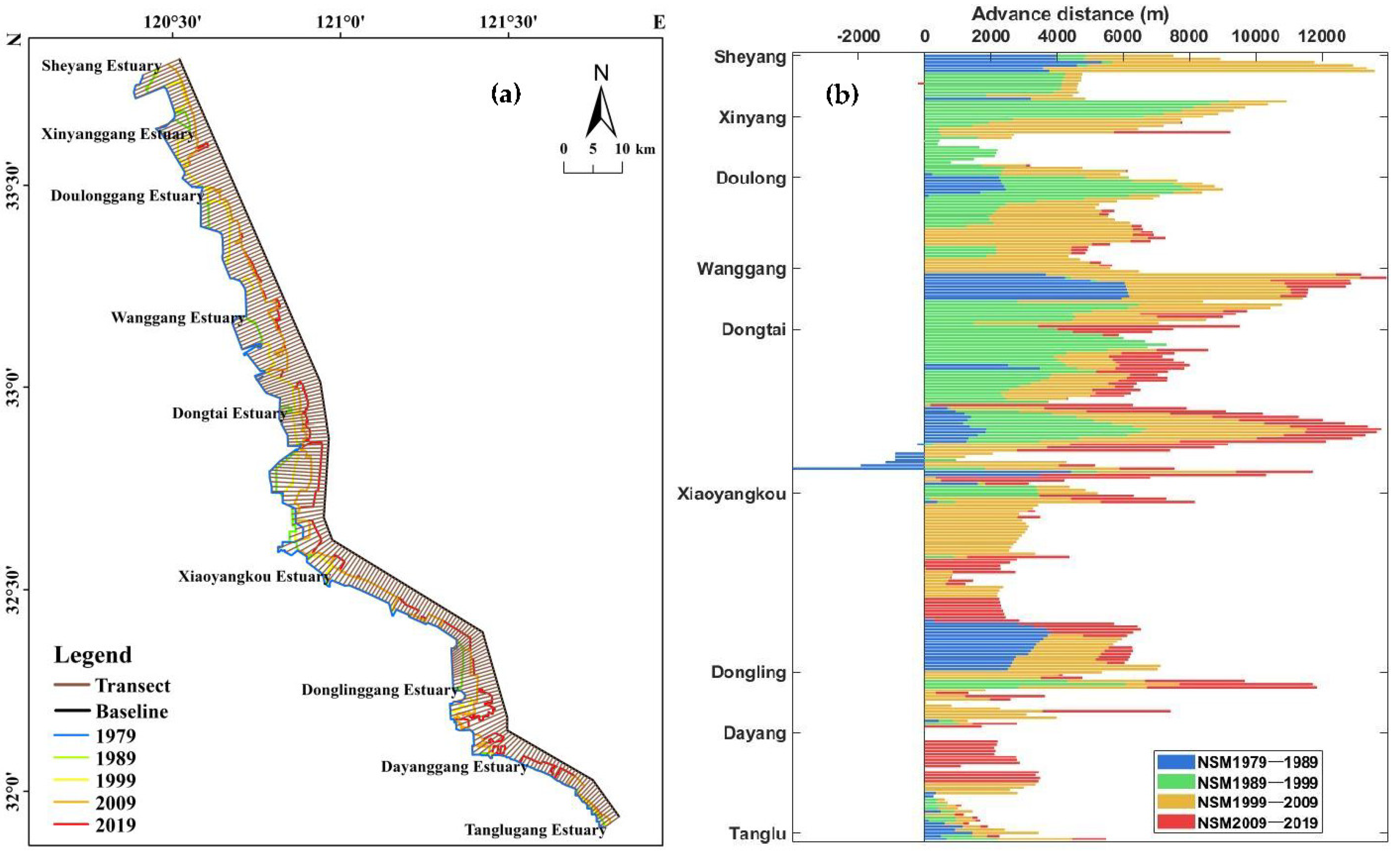
Long-term change of artificial shorelines from 1979 to 2019 was analyzed based on DSAS, as shown in Figure 6. According to the t (NSM) result, the coastline has been advancing towards the sea from Sheyang to Tanglugang estuary. The maximum advance rate was 348.76 m/a, and the average was 136.98 m/a. In general, the shoreline changed dramatically from Wanggang to Xiaoyangkou estuary compared with other areas. The annual change rate of the coastline from 1979 to 1989 was 65.92 m/a, from 1989 to 1999 it exceeded 150 m/a, from 1999 to 2009 it was about 226.58 m/a, and from 2009 to 2019 it was 102 m/a. The period from 2009 to 2019 showed the fastest rate of advance to the sea, due to frequent reclamation activities.
4.2. Evolution Analysis of Exposed Tidal Flat
4.2.1. Area Change of Exposed Tidal Flats
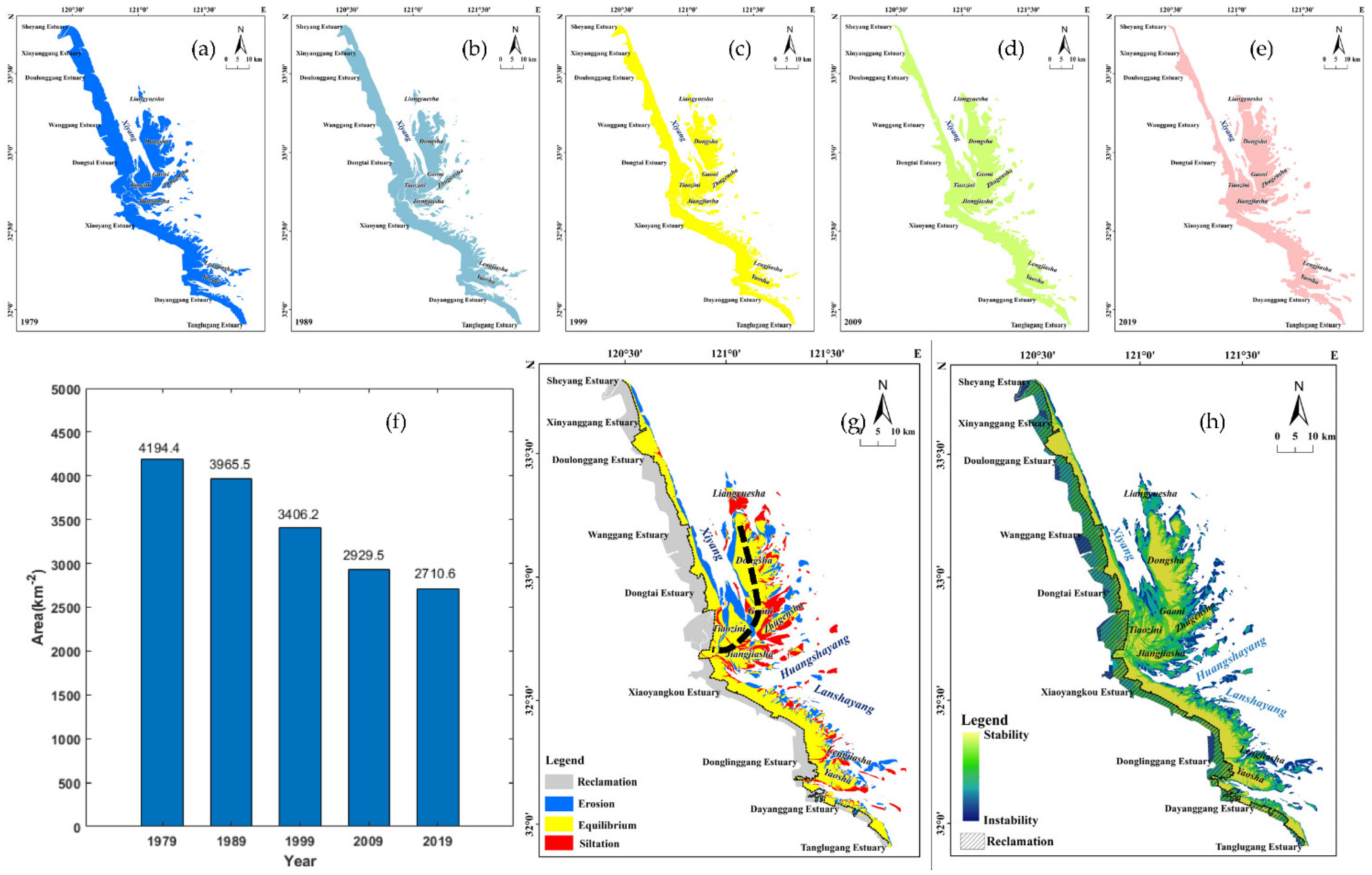
Based on the extraction of the waterlines and the vector polygon merging, five distribution surfaces of the exposed tidal flats were obtained during the period of 1979–2019 (Figure 7a–e). Based on GIS spatial statistical analysis, the area of exposed tidal flats in the RSRs was calculated. As shown in Figure 7f, over the past 40 years, the area has decreased by 1484 km2. The change of tidal flat area was rapid in the first 30 years but relatively slow in the last 10 years. Except for the reclaimed area of 1414 km2, the area of exposed tidal flat has decreased only by 70 km2. The results showed that in the past 40 years, the exposed tidal flats of RSRs have not changed much under natural conditions, and the decrease in area is mainly due to reclamation activities in high tidal flats.
4.2.2. Stability Analysis of Exposed Tidal Flats
Based on five-period tidal flat polygon layers (Figure 7a–e), spatial overlay analysis was executed to analyze the stability of exposed tidal flats using ArcGIS software. The overlay map between 1979 and 2019 (Figure 7g) bounded by the black dotted line showed a trend of erosion in the north around Xiyang channel and deposition in the southeast around Gaoni and Jiangjiasha sand ridges. Tidal flats have shown a trend of moving southwest in the past 40 decades. For example, Erfenshui of Tiaozini has moved 11 km southward, while distances of 8 km for Liangyuesha and 5 km for Lengjiasha were also observed.
In addition, based on five polygon layers of exposed tidal flats (Figure 7a–e), the number of occurrences was used as the main indicator of stability assessment, and the union tool was used to obtain the stability map of tidal flats (Figure 7h). The more occurrences, the higher the tidal flat stability; the fewer occurrences, the worse the tidal flat stability. The result showed that regarding the large-scale sandbanks of the RSRs, the stability of Dongsha and the coastal beaches (outside Doulong Port, Xiaoyangkou−Daiyang Port) is relatively high. Tiaozini and Gaoni are obviously affected by tidal creeks, and their stability plaques are more fragmented.
4.3. Analysis of Geomorphic Evolution of Sand Ridge
4.3.1. Spatial Distribution Characteristics of RSRs
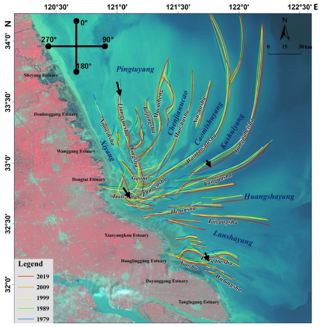
The sand ridge lines of five different periods (1979–2019) were extracted, and the overlay map is shown in Figure 8. The average length of the ridgeline and the average direction angle were calculated and are shown in Table 2. The result showed that radial sand ridges (RSRs) spread in a fan-shaped pattern over the seabed of the Southern Yellow Sea are divided into two regions, the south and the north, which are bounded by the Huangshayang channel. The northern region can be further divided into the northeast region and the northwest region. In the northeast, there are large-scale sandbanks in the northeast, such as Macaiheng, Mozhusha, Waimozhusha, and Jiangjiasha, which are more than 100 km in length. The direction of the sand ridges in this area varies from 10° to 71°, with an average of 30°. In the northwest area, the sand ridges mainly include Dongsha, Gaoni, and Xiaoyinsha with a length of around 80 km. The direction of the sand ridge is basically true north. In the southern region, shorter sand ridges (within 50 km) are distributed here. The main sand ridges are Hetunsha, Taiyangsha, Lengjiasha, and Yaosha with direction varying from 80° to 120°, with an average of 100°.
The comparison of sand ridge lines in five different periods shows that, in the past 40 years, the sand ridges of the RSRs have been radiating out to the sea. With the passage of time, the sand ridge lines in the RSRs are generally in the north–south direction, among which Tiaozini and Yaosha were the most typical ones. The outer sea sand ridge is bounded by Kushuiyang, the north–south fan angle has a trend of increasing, and the southern sandbar of Kushuiyang has an obvious trend of southward movement.
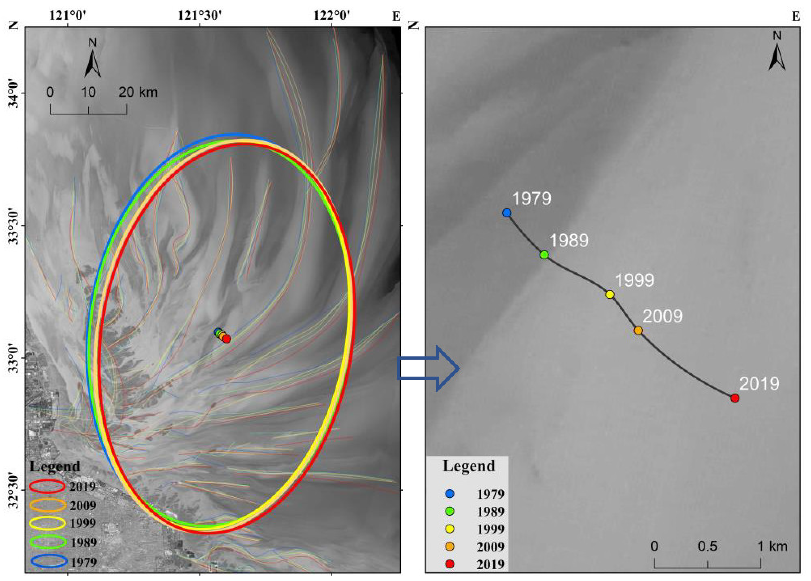
4.3.2. Movement Trend of Sand Ridges
The standard deviational ellipse method was used to analyze the change of sand ridge lines. As shown in Figure 9, standard deviation ellipses and geographic centers in different periods were obtained, and morphological parameters were counted (Table 3). Overall, the shape of the directional ellipse has not changed much in the past 40 years, and the change range of the major axis and the minor axis are both within 5%, indicating that the overall radial shape of the sand ridge group is relatively stable. However, the center point of ellipse showed a trend of gradually moving southeast (Table 4). From 1979 to 2019, the moving distance is nearly 4 km, and the direction is southeast (135°), with an average annual movement of 100 m. Compared with other periods, the movement of sand ridges has accelerated in the last 10 years (2009–2019).
5. Discussion
5.1. Causes and Future Trend of the Shoreline
From 1979 to 2019, the shoreline of the RSRs has shown a clear trend of advancing toward the sea. Undoubtedly, the reclamation of tidal flats is the main reason. More than 1400 km2 of tidal flats have been gradually reclaimed in the past 40 years, and the next 1 million mu (667 km2) tidal flats reclamation plan was launched in 2010 [39] (Figure 10a). However, in the past 10 years, with the background of the construction of China’s marine ecological civilization, more attention has gradually been paid to the protection of tidal flats. In 2018, the State Council of China issued the ‘Notice on Strengthening the Protection of Coastal Wetlands and Strictly Controlling Reclamation’ (hereinafter referred to as the ‘Notice’) [40]. The ‘Notice’ requires that the total control of the total amount of reclamation be improved and the annual plan targets for local reclamation and reclamation will be cancelled. Except for strategic projects, the approval of new reclamation projects will be completely stopped. Immediately afterwards, in 2019, China’s migratory bird sanctuaries along the coast of the Yellow Sea–Bohai Gulf (Phase I) were inscribed on the World Heritage List as a natural site at the forty-third session of the UNESCO World Heritage Committee in Azerbaijan’s capital [6]. Therefore, in this context, it is unlikely that the shoreline will be pushed to the sea due to reclamation in the future, except for certain large-scale port constructions (such as Tongzhouwan Port).
5.2. Driving Forces for the Southeastward Movement of the RSRs
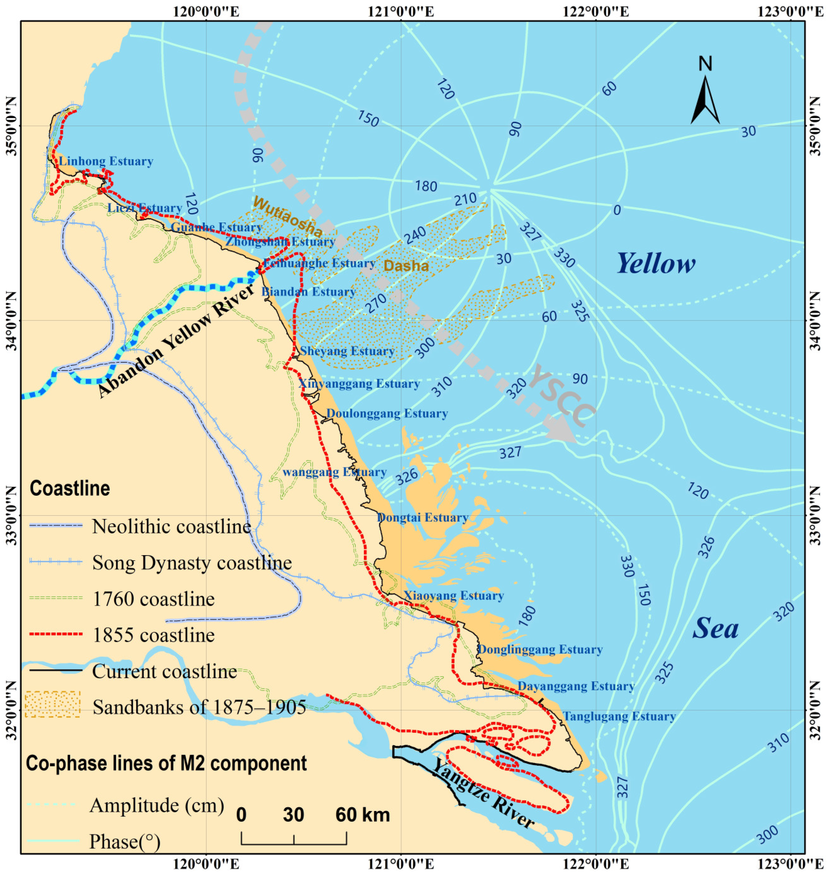
According to the previous results, in the past 40 years, the RSRs including exposed tidal flats and underwater sand ridges have shown a trend of moving to the southeast direction, such as Tiaozini where the center area of the RSRs has moved south by 11 km as shown in Figure 8. What caused this obvious trend of RSRs? For thousands of years, the coast of Jiangsu has undergone tremendous changes in the sea [41], but the convergent and divergent tidal wave system has always existed. With a huge amount of sediment replenishment [6], it has been transforming the landform of the RSRs. The evolution of RSRs is the result of both external and internal influences. Firstly, from the perspective of the external macro-dynamic conditions of the Yellow Sea, for decades, it has been believed that there is a southward coastal current in the southwestern part of the Yellow Sea (Figure 11), which is called the Yellow Sea Coastal Current (YSCC). It is the common direction of coastal currents under geostrophic balance and is also the downwind direction under the prevailing East Asian monsoon in winter [42]. Secondly, in the inner RSRs, the north area around Xiyang channel, the tidal currents almost follow a straight route also because of the narrower troughs. Measured tidal current velocities can reach 3.12 m/s [12]. In the south area around Lanshayang−Huangshayang, the tidal current vector ellipses are mostly egg-shaped and tidal velocity is 0.5~0.8 m/s. The residual flow value varies from 0.007 to 0.37 m/s, and the direction of residual flow is not obvious, but it is consistent with the direction of the sandbank and the tidal channel. Due to poor depth measurements, complex tides, and harsh sea conditions, there are few direct measured data. The dynamic conditions and mechanisms of this sea area need further discussion. However, previous studies have revealed that tidal currents play a dominant role in the formation and development of the RSRs, while the contributions of storms/waves are secondary [7,17]. The convergent tidal wave system (propagating tidal wave from the south and the rotational tidal wave system from the north [32]) is the inevitable result of tide waves propagating under the unique boundary formed by the Korean Peninsula, Shandong Peninsula, and Jiangsu coastline (Figure 11). Large changes in ocean tidal waves, Coriolis force, deep sea topography and friction coefficients were unlikely to change much in the past 40 years. Existing numerical simulation studies have shown that this convergent−divergent tidal wave system has existed stably for thousands of years. The local changes of Jiangsu coastline and topographical changes only affect the local tidal wave energy [43,44]. The Yellow River seized the Huaihe River into the sea in 1128, the Jiangsu coast was silted out for 60 km overall as shown in Figure 11. Before the Yellow River returned to the north in 1855, the abandoned Yellow River coastline protruded to the sea more than 20 km. In addition, there was a huge underwater delta (Wutiaosha and Dasha sandbank are shown as of 1875–1905 [6]), which blocked the rotating tidal wave propagating from north to south, and the hydrodynamic force was relatively weak. After the Yellow River returned to the north, as the shoreline retreated and the underwater delta eroded, deposition continued along the Dafeng–Dongtai line [45], the rotating tidal wave became smoother, and the hydrodynamic force of the RSRs sea area was further strengthened. In addition to the changes in coastal location, in the past 40 years, under the influence of human activities, the coastline of Central Jiangsu has gradually evolved from its original natural rough shape to an artificially straight shape [13], making the reflection of tidal waves stronger and more direct. Furthermore, from the perspective of hydrodynamics, Ni et al., proposed that tidal waves propagate in the offshore tidal channel−sand ridge system and generate a residual current circulation around the sand ridge [46]. Residual currents drive sediment transport. There is a spatial gradient between tidal channel and sand ridge, which leads to accretion on the south side and erosion on the north side. As a result, the sand ridges migrate southward.
Therefore, we infer that the strengthening of this regional tidal wave system to the south and east may be one of the leading factors that caused the radiation sandbank to move southeast. In the future, the trend of southeastward movement of the radial sand ridge group will still exist. With the background of enhanced dynamics, the topographic difference between sand ridges and deep troughs will further increase, and the topography will become steeper. For example, in the northern section of Tiaozini in the Xiyang Channel, the multi-year elevation curve shows great changes. The interaction between hydrodynamic changes and coastal evolution has existed for a long time, and coastal changes cause tidal wave changes. At the same time, the changed tidal wave system distribution will also reshape coastal landforms.
5.3. Limitations for the Geomorphic Evolutionary Analysis of the Radial Sand Ridges
In terms of image processing, atmospheric correction was not performed in this study, because the parameters of the radiation transfer model were difficult to obtain. In the future, we will increase observations and develop the atmospheric correction model suitable for Jiangsu offshore waters. In addition, the time span of this study was 40 years, but there were only five-time nodes, and the interval of each time node was 10 years, which is too long to obtain detailed geomorphic information of RSRs. In the future, we can shorten the time interval and refine the analysis of the evolution characteristics of the RSRs. In addition, due to the lack of measured topographic data, this study used the waterlines and underwater sand ridgelines to characterize the entire seabed and lacks a quantitative analysis of three-dimensional erosion and deposition. In the future, we will try to build an underwater terrain remote sensing inversion model and quantitatively analyze the geomorphic evolution of RSRs by constructing serial digital elevation models of tidal flats and underwater sand ridges.
6. Conclusions
The RSRs of the South Yellow Sea, as a sensitive zone, are bearing the dual pressure from land and sea. This study made full use of the multi-source remote sensing data from 1979 to 2019, took the geomorphological feature line (shoreline, waterline, and sand ridge line) as the description object, and analyzed the geomorphic evolution of the RSRs quantitatively and finely using GIS spatial analysis technology.
The main findings are as follows:
- (1)
- The coastline has been advancing towards the sea from the Sheyang to Tanglugang estuary. The maximum advance rate was 348.76 m/a, and the average was 136.98 m/a. The section from Wanggang to Xiaoyang Port advances the most to the sea, and 1999–2009 is the period with the fastest advancing rate. The large-scale reclamation in Jiangsu province is the main driving force;
- (2)
- The exposed tidal flat area has decreased sharply, and the offshore sandbars have moved significantly to the southeast. Over the past 40 years, the exposed tidal flats have decreased by 1484 km2 including the reclaimed area of 1414 km2 and have showed a trend of erosion in the north around Xiyang channel and deposition in the southeast around the Gaoni and Jiangjiasha areas;
- (3)
- RSRs have been spread in a fan-shaped pattern over the seabed of the Southern Yellow Sea in the past 40 years with pronounced differences between the northern and southern channel−sand ridges. From 1979 to 2019, the sand ridge lines showed a trend of gradually moving southeast, the moving distance is nearly 4 km, and the direction is southeast (135°), with an average annual movement of 100 m. The enhancement of the northern rotating tidal wave system may be one of the leading factors.
Author Contributions
Conceptualization, Y.K. and J.H.; methodology, Y.K; software, J.H. and B.W.; validation, B.W. and X.D.; formal analysis, J.L.; investigation, J.L. and Z.W.; resources, Y.K.; data curation, Y.K.; writing—original draft preparation, J.H. and Y.K.; writing—review and editing, Y.K. All authors have read and agreed to the published version of the manuscript.
Funding
This research was funded by the National Key R&D Program of China (2018YFD0900906); National Natural Science Funds of China (41806118, 41976163); Major International (Regional) Joint Research Project (51620105005); Jiangsu Transportation Technology Project (2017ZX01); and the Jiangsu Marine Science and Technology Innovation Project (HY2017−6).
Data Availability Statement
The data presented in this research are available upon request from the corresponding authors.
Acknowledgments
The authors are grateful to the China Center for Resource Satellite Data and Applications (CRESDA) for supplying all the HJ−1 CCD and GF−1 images. Thanks to the United States Geological Survey (USGS) for providing Landsat images. Thanks to Gong Zheng, Tao Jianfeng, Zhang Changkuan, Xu Qing and Su min for their suggestions and support during the research process. We thank Ren Limin, Mao Zhibin, Miao Zhihong, and Sun Yulong who participated in the field work for the establishment of five tide-gauge stations.
Conflicts of Interest
The authors declare no conflict of interest.
References
- Wang, Y.; Zhang, Y.; Zou, X.; Zhu, D.; Piper, D. The sand ridge field of the South Yellow Sea: Origin by river–sea interaction. Mar. Geol. 2012, 291–294, 132–146. [Google Scholar] [CrossRef]
- Jian, L.; Saito, Y.; Kong, X.; Hong, W.; Xiang, L.; Wen, C.; Nakashima, R. Sedimentary record of environmental evolution off the Yangtze River estuary, East China Sea, during the last 13,000 years, with special reference to the influence of the Yellow River on the Yangtze River delta during the last 600 years. Quat. Sci. Rev. 2010, 29, 2424–2438. [Google Scholar]
- UNESCO World Heritage Centre. Available online: https://whc.unesco.org/en/sessions/43COM/ (accessed on 23 July 2019).
- Chen, W.T.; Zhang, D.; Hong-Yi, L.I.; Han, F.; Geography, D.O.; University, N.N. Quantitative Assessment of Reclamation Intensity and Development Potential in the Onshore Coast of Radial Sandbank. Adv. Mar. Sci. 2017, 35, 295–304. [Google Scholar]
- Shen, F.; Zhou, Y.; Li, J.; He, Q.; Verhoef, W. Remotely sensed variability of the suspended sediment concentration and its response to decreased river discharge in the Yangtze estuary and adjacent coast. Cont. Shelf Res. 2013, 69, 52–61. [Google Scholar] [CrossRef]
- Zhou, L.; Liu, J.; Saito, Y.; Zhang, Z.; Chu, H.; Hu, G. Coastal erosion as a major sediment supplier to continental shelves: Example from the abandoned Old Huanghe (Yellow River) delta. Cont. Shelf Res. 2014, 82, 43–59. [Google Scholar] [CrossRef]
- Su, M.; Yao, P.; Wang, Z.B.; Zhang, C.K.; Stive, M.J.F. Exploratory morphodynamic modeling of the evolution of the Jiangsu coast, China, since 1855: Contributions of old Yellow River-derived sediment. Mar. Geol. 2016, 390, 306–320. [Google Scholar] [CrossRef]
- Wang, Y.; Liu, Y.; Jin, S.; Sun, C.; Wei, X. Evolution of the topography of tidal flats and sandbanks along the Jiangsu coast from 1973 to 2016 observed from satellites. ISPRS J. Photogramm. 2019, 150, 27–43. [Google Scholar] [CrossRef]
- Dyer, K.R.; Huntley, D.A. The origin, classification and modelling of sand banks and ridges. Cont. Shelf Res. 1999, 19, 1285–1330. [Google Scholar] [CrossRef]
- Ren, M. Comprehensive Investigation of Coastal Zone and Tidal Flat Resources, Jiangsu Province; Ocean Press: Beijing, China, 1986. (In Chinese) [Google Scholar]
- Zhang, R. Evolution of Sand Bodies in Jiangsu Offshore Zone and Prospect of ‘Tiaozini’ Advancing to Land; Ocean Press: Beijing, China, 1992. (In Chinese) [Google Scholar]
- Zhang, C. Comprehensive Investigation and Assessment Report of Jiangsu Offshore; China Science Press: Beijing, China, 2012. (In Chinese) [Google Scholar]
- Wang, Y.P.; Gao, S.; Jia, J.; Thompson, C.; Gao, J.; Yang, Y. Sediment transport over an accretional intertidal flat with influences of reclamation, Jiangsu coast, China. Mar. Geol. 2012, 291–294, 147–161. [Google Scholar] [CrossRef]
- Gong, Z.; Jin, C.; Zhang, C.; Zhou, Z.; Zhang, Q.; Li, H. Temporal and spatial morphological variations along a cross-shore intertidal profile, Jiangsu, China. Cont. Shelf Res. 2017, 144, 1–9. [Google Scholar] [CrossRef]
- Choi, J.K.; Ryu, J.H.; Lee, Y.K.; Yoo, H.R.; Han, J.W.; Chang, H.K. Quantitative estimation of intertidal sediment characteristics using remote sensing and GIS. Estuar. Coast. Shelf Sci. 2010, 88, 125–134. [Google Scholar] [CrossRef]
- Xu, F.; Tao, J.; Zhou, Z.; Coco, G.; Zhang, C. Mechanisms underlying the regional morphological differences between the northern and southern radial sand ridges along the Jiangsu Coast, China. Mar. Geol. 2016, 371, 1–17. [Google Scholar] [CrossRef]
- Tao, J.; Wang, Z.B.; Zhou, Z.; Xu, F.; Stive, M.J.F. A Morphodynamic Modeling Study on the Formation of the Large-cale Radial Sand Ridges in the Southern Yellow Sea. J. Geophys. Res. Earth Surf. 2019, 124, 1742–1761. [Google Scholar] [CrossRef]
- Zhang, W.; Zhang, X.; Huang, H.; Wang, Y.; Fagherazzi, S. On the morphology of radial sand ridges. Earth Surf. Process. Landf. 2020, 45, 2613–2630. [Google Scholar] [CrossRef]
- Zhou, Z.; Mick, V.D.W.; Jagers, B.; Coco, G. Modelling the role of self-weight consolidation on the morphodynamics of accretional mudflats. Environ. Modell. Softw. 2016, 76, 167–181. [Google Scholar] [CrossRef]
- Randazzo, G.; Italiano, F.; Micallef, A.; Tomasello, A.; Cassetti, F.P.; Zammit, A.; D’Amico, S.; Saliba, O.; Cascio, M.; Cavallaro, F.; et al. WebGIS Implementation for Dynamic Mapping and Visualization of Coastal Geospatial Data: A Case Study of BESS Project. Appl. Sci. 2021, 11, 8233. [Google Scholar] [CrossRef]
- Bezzi, A.; Casagrande, G.; Fracaros, S.; Martinucci, D.; Pillon, S.; Sponza, S.; Bratus, A.; Fattor, F.; Fontolan, G. Geomorphological Changes of a Migrating Sandbank: Multidecadal Analysis as a Tool for Managing Conflicts in Coastal Use. Water 2021, 13, 3416. [Google Scholar] [CrossRef]
- Salameh, E.; Frappart, F.; Almar, R.; Baptista, P.; Laignel, B. Monitoring Beach Topography and Nearshore Bathymetry Using Spaceborne Remote Sensing: A Review. Remote Sens. 2019, 11, 2212. [Google Scholar] [CrossRef] [Green Version]
- Murray, N.J.; Phinn, S.R.; Clemens, R.S.; Roelfsema, C.M.; Fuller, R.A. Continental Scale Mapping of Tidal Flats across East Asia Using the Landsat Archive. Remote Sens. 2012, 4, 3417–3426. [Google Scholar] [CrossRef] [Green Version]
- Jia, M.; Wang, Z.; Mao, D.; Ren, C.; Wang, Y. Rapid, robust, and automated mapping of tidal flats in China using time series Sentinel-2 images and Google Earth Engine. Remote Sens. Environ. 2021, 255, 112285. [Google Scholar] [CrossRef]
- Mason, D.C.; Scott, T.R.; Dance, S.L. Remote sensing of intertidal morphological change in Morecambe Bay, U.K., between 1991 and 2007. Estuar. Coast. Shelf Sci. 2010, 87, 487–496. [Google Scholar] [CrossRef] [Green Version]
- Ryu, J.H.; Kim, C.H.; Lee, Y.K.; Won, J.S.; Chun, S.S.; Lee, S. Detecting the intertidal morphologic change using satellite data. Estuar. Coast. Shelf Sci. 2008, 78, 623–632. [Google Scholar] [CrossRef]
- Liu, Y.X.; Li, M.C.; Zhou, M.X.; Kang, Y.; Mao, L. Quantitative Analysis of the Waterline Method for Topographical Mapping of Tidal Flats: A Case Study in the Dongsha Sandbank, China. Remote Sens. 2013, 5, 6138–6158. [Google Scholar] [CrossRef] [Green Version]
- Zhao, B.; Guo, H.; Yan, Y.; Wang, Q.; Bo, L. A simple waterline approach for tidelands using multi-temporal satellite images: A case study in the Yangtze Delta. Estuar. Coast. Shelf Sci. 2008, 77, 134–142. [Google Scholar] [CrossRef]
- Wang, Y.; Zhu, D.; You, K.; Pan, S.; Zhu, X.; Zou, X.; Zhang, Y. Evolution of radiative sand ridge field of the South Yellow Sea and its sedimentary characteristics. Sci. China Ser. D 1999, 42, 97–112. [Google Scholar] [CrossRef]
- Yao, P.; Su, M.; Wang, Z.; Rijn, L.V.; Zhang, C.; Chen, Y.; Stive, M. Experiment inspired numerical modeling of sediment concentration over sand–silt mixtures. Coast. Eng. 2015, 105, 75–89. [Google Scholar] [CrossRef]
- Liu, T.; Shi, X.; Chaoxin, L.I.; Yang, G. The reverse sediment transport trend between abandoned Huanghe River (Yellow River) Delta and radial sand ridges along Jiangsu coastline of China—An evidence from grain size analysis. Acta Oceanol. Sin. 2012, 31, 83–91. [Google Scholar] [CrossRef]
- Zhang, C. Tidal current-induced formation-storm-induced change-tidal current-induced recovery-Interpretation of depositional dynamics of formation and evolution of radial sand ridges on the Yellow Sea seafloor. Sci. China Ser. D Earth Sci. 1999, 1, 1–12. [Google Scholar] [CrossRef]
- Kang, Y.; Ding, X.; Xu, F.; Zhang, C.; Ge, X. Topographic mapping on large-scale tidal flats with an iterative approach on the waterline method. Estuar. Coast. Shelf Sci. 2017, 190, 11–22. [Google Scholar] [CrossRef]
- Thieler, E.R.; Himmelstoss, E.A.; Zichichi, J.L.; Ergul, A. The Digital Shoreline Analysis System (DSAS) Version 4.0—An ArcGIS Extension for Calculating Shoreline Change; U.S. Geological Survey: Reston, VA, USA, 2009; pp. 1278–2008. [Google Scholar]
- Ryu, J.H.; Won, J.S.; Min, K.D. Waterline extraction from Landsat TM data in a tidal flat: A case study in Gomso Bay, Korea. Remote Sens. Environ. 2002, 83, 442–456. [Google Scholar] [CrossRef]
- Bhaskaran, S.; Paramananda, S.; Ramnarayan, M. Per-pixel and object-oriented classification methods for mapping urban features using Ikonos satellite data. Appl. Geogr. 2010, 30, 650–665. [Google Scholar] [CrossRef]
- Mao, Z.; Chen, J.; Pan, D.; Tao, B.; Zhu, Q. A regional remote sensing algorithm for total suspended matter in the East China Sea. Remote Sens. Environ. 2012, 124, 819–831. [Google Scholar] [CrossRef]
- Yuill, R.S. The Standard Deviational Ellipse; An Updated Tool for Spatial Description. Geogr. Ann. Ser. B Hum. Geogr. 1971, 53, 28–39. [Google Scholar] [CrossRef]
- Zhang, C.; Chen, J.; Lin, K.; Ding, X.; Yuan, R.; Kang, Y. Spatial layout of reclamation of coastal tidal flats in Jiangsu Province. J. Hohai Univ. 2011, 39, 206–212. (In Chinese) [Google Scholar]
- The State Council of the People’s Republic of China. Available online: http://www.gov.cn/zhengce/content/2018-07/25/content_5309058.htm (accessed on 25 July 2010).
- Zhang, R. Coastline changes in Jiangsu province during historical period. In Proceedings of Quaternary Coastline Symposium, China, 1982; China Quaternary Research Association and Chinese Society of Oceanography, Ed.; China Ocean Press: Beijing, China, 1985; pp. 132–145. (In Chinese) [Google Scholar]
- Wu, H.; Gu, J.; Zhu, P. Winter counter-wind transport in the inner southwestern Yellow Sea. J. Geophys. Res. Ocean 2018, 123, 411–436. [Google Scholar] [CrossRef]
- Gao, S.; Collins, M.B. Holocene sedimentary systems on continental shelves. Mar. Geol. 2014, 352, 268–294. [Google Scholar] [CrossRef]
- Chen, K.F.; Wang, Y.H.; Lu, P.D.; Zheng, J.H. Effects of Coastline Changes on Tide System of Yellow Sea off Jiangsu Coast, China. China Ocean Eng. 2009, 23, 741–750. [Google Scholar]
- Kang, Y.; Xia, F.; Ding, X.; Zhang, C.; Cheng, L.; Ge, X.; Glass, J. Coastal evolution of Yancheng, northern Jiangsu, China since the mid-Holocene based on the Landsat MSS imagery. J. Geogr. Sci. 2013, 23, 915–931. [Google Scholar] [CrossRef]
- Ni, W.; Wang, Y.; Zou, X.; Zhang, J.; Gao, J. Sediment dynamics in an offshore tidal channel in the southern Yellow Sea. Int. J. Sediment Res. 2014, 29, 246–259. [Google Scholar] [CrossRef]
Figure 1.
Location and topographic map of the RSRs.

Figure 2.
Remote sensing images of artificial shorelines. (a) Dike or breakwater in MSS (654) image; (b) dock in TM (432) image; (c) estuary in HJ−1(432) image; (d) breeding ponds in OLI (543) image.
Figure 2.
Remote sensing images of artificial shorelines. (a) Dike or breakwater in MSS (654) image; (b) dock in TM (432) image; (c) estuary in HJ−1(432) image; (d) breeding ponds in OLI (543) image.

Figure 3.
Waterline extraction flow diagram using the object-oriented classification method.

Figure 4.
Sand ridge line extraction flow diagram.

Figure 5.
Comparison with surveyed data and extracted image of sand ridge lines; (a) digital elevation model (DEM) based on surveyed data; (b) overlay map of image and contours of DEM.
Figure 5.
Comparison with surveyed data and extracted image of sand ridge lines; (a) digital elevation model (DEM) based on surveyed data; (b) overlay map of image and contours of DEM.

Figure 6.
(a) Shorelines, baselines, and transects of the RSRs; (b) t (NSM) of shoreline in different periods of the RSRs from 1979 to 2019.
Figure 6.
(a) Shorelines, baselines, and transects of the RSRs; (b) t (NSM) of shoreline in different periods of the RSRs from 1979 to 2019.

Figure 7.
(a–e) Distribution map of exposed tidal flats from 1979–2019; (f) area comparison between five periods; (g) overlay map between 1979 and 2019; (h) stability spatial distribution map based on overlay analysis of five polygon layers (a–e).
Figure 7.
(a–e) Distribution map of exposed tidal flats from 1979–2019; (f) area comparison between five periods; (g) overlay map between 1979 and 2019; (h) stability spatial distribution map based on overlay analysis of five polygon layers (a–e).

Figure 8.
Spatial overlay map of sand ridge lines from 1979 to 2019.

Figure 9.
Ellipse and geographic center changes of the RSRs during 1979–2019.

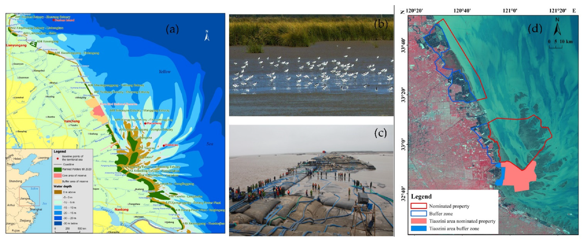
Figure 10.
(a) planed polders in Jiangsu Tidal Flats [39]; (b) tidal flat birds; (c) reclamation photo; (d) the two components of the migratory bird sanctuaries along the Coast of Yellow Sea–Bohai Gulf of China (Phase I) [6].

Figure 11.
Historical shoreline evolution and tidal wave system. The historical shorelines are collected from Zhang 1985 [41]; subwater sandbanks are collected from Zhou et al. 2014 [6]; co-phase lines of M2 component in southern yellow sea are collected from Xu et al. 2016 [16].


Table 1.
Remote sensing images and corresponding tide level data.
| Object Extraction | Date | Satellite | Sensor | Tide Level/m (CNHD 1985) | ||||
|---|---|---|---|---|---|---|---|---|
| DFG | DSG | DDG | TYG | YKG | ||||
| waterline | 1978/05/11 | Landsat-2 | MSS | −1.98 | −2.03 | −3.12 | −2.25 | −1.94 |
| waterline | 1978/08/09 | Landsat-2 | MSS | −2.37 | −2.00 | −2.89 | −1.79 | −2.40 |
| waterline | 1978/08/10 | Landsat-2 | MSS | −2.32 | −1.86 | −2.45 | −1.42 | −2.40 |
| waterline | 1978/09/05 | Landsat-2 | MSS | −1.49 | −2.07 | −3.30 | −2.73 | −1.49 |
| shoreline | 1979/09/09 | Landsat-2 | MSS | −2.17 | −2.1 | −2.33 | −1.32 | −1.75 |
| waterline/sand ridge line | 1979/09/10 | Landsat-2 | MSS | −2.45 | −2.36 | −2.30 | −2.04 | −2.24 |
| waterline | 1980/09/30 | Landsat-2 | MSS | −2.05 | −1.34 | −2.99 | −2.29 | −1.9 |
| waterline | 1980/10/28 | Landsat-2 | MSS | −1.85 | −1.55 | −3.26 | −2.62 | −1.82 |
| waterline | 1980/12/12 | Landsat-2 | MSS | −1.89 | −1.54 | −2.08 | −1.42 | −1.83 |
| waterline | 1988/03/08 | Landsat-5 | TM | −2.09 | −1.31 | −2.60 | −1.89 | −1.85 |
| waterline | 1988/06/05 | Landsat-5 | TM | −2.27 | −1.81 | −2.82 | −1.84 | −2.56 |
| waterline | 1989/03/27 | Landsat-5 | TM | −2.34 | −1.20 | −2.94 | −2.10 | −2.05 |
| shoreline/sand ridge line | 1989/12/01 | Landsat-5 | TM | −1.49 | −1.06 | −1.46 | −1.20 | −2.25 |
| waterline | 1990/04/15 | Landsat-5 | TM | −1.91 | −1.15 | −3.32 | −2.77 | −1.89 |
| waterline | 1990/07/13 | Landsat-5 | TM | −2.65 | −2.06 | −3.21 | −1.91 | −2.81 |
| waterline | 1998/01/31 | Landsat-5 | TM | −1.47 | −3.02 | −3.06 | −3.14 | −1.63 |
| shoreline/sand ridge line | 1999/02/19 | Landsat-5 | TM | 0.95 | −2.59 | −2.33 | −3.93 | −1.53 |
| waterline | 2000/03/09 | Landsat-5 | TM | −2.02 | −1.36 | −2.66 | −1.97 | −1.34 |
| waterline | 2000/03/26 | Landsat-7 | ETM+ | −2.22 | −1.21 | −2.57 | −1.80 | −2.21 |
| waterline | 2000/04/10 | Landsat-5 | TM | −2.42 | −1.65 | −3.05 | −2.02 | −2.53 |
| waterline | 2000/06/06 | Landsat-5 | TM | −2.32 | −1.89 | −2.53 | −1.49 | −2.33 |
| waterline | 2000/09/18 | Landsat-7 | ETM+ | −1.59 | −1.72 | −2.78 | −2.25 | −1.51 |
| waterline | 2000/10/04 | Landsat-7 | ETM+ | −1.39 | −0.61 | −2.56 | −2.50 | −1.2 |
| waterline | 2008/02/12 | Landsat-5 | TM | −1.92 | −1.58 | −2.89 | −2.12 | −2.35 |
| waterline | 2008/05/11 | Landsat-5 | TM | −2.34 | −2.36 | −2.53 | −1.33 | −2.02 |
| shoreline/waterline | 2009/04/28 | Landsat-5 | TM | −2.25 | −0.83 | −2.57 | −1.90 | −1.52 |
| sand ridge line | 2009/05/29 | Landsat-7 | ETM+ | −2.39 | −1.85 | −1.57 | −1.50 | −2.42 |
| shoreline | 2009/06/14 | Landsat-7 | ETM+ | −2.11 | −1.7 | −1.36 | −1.51 | −2.23 |
| waterline | 2009/08/26 | Landsat-5 | ETM+ | −2.18 | −1.51 | −1.09 | −2.26 | −1.89 |
| waterline | 2010/12/26 | Landsat-7 | TM | −1.65 | −1.77 | −1.46 | −1.88 | −2.2 |
| waterline | 2010/12/27 | Landsat-7 | TM | −1.02 | −1.74 | −1.42 | −1.25 | −2.17 |
| waterline | 2018/03/23 | HJ-1 | CCD | −2.52 | −2.25 | −2.97 | −1.70 | −2.79 |
| waterline | 2018/07/18 | Landsat-7 | ETM+ | −2.21 | −2.24 | −3.25 | −2.84 | −2.73 |
| waterline | 2019/03/13 | HJ-1 | WFV | −2.43 | −2.14 | −2.73 | −2.89 | −2.42 |
| shoreline | 2019/03/15 | GF-1 | CCD | −1.73 | −1.7 | −2.06 | −1.88 | −1.57 |
| sand ridge line | 2019/05/21 | HJ-1 | CCD | 0.02 | −1.09 | −2.43 | −2.45 | −1.46 |
| waterline | 2019/06/08 | GF-1 | WFV | −0.66 | −1.18 | −2.82 | −2.93 | −1.92 |
| waterline | 2019/08/21 | Landsat-8 | OLI | −0.72 | −1.42 | −2.62 | −2.51 | −1.56 |
Table 2.
Statistical table of morphological parameters of sand ridges.
| Sand Ridges | Length (km) | Direction (°) | Sand Ridges | Length (km) | Direction (°) |
|---|---|---|---|---|---|
| Gaoni−Dongsha | 96 | 350 | Tiaozini−Jiangjiasha | 135 | 71 |
| Macaiheng | 70 | 10 | Hetunsha | 38 | 80 |
| Maozhusha | 111 | 26 | Tangyangsha | 60 | 95 |
| Waimaozhusha | 185 | 18 | Lengjiasha | 51 | 105 |
| Jiangjiabeisha | 156 | 27 | Yaosha−Wulongsha | 54 | 120 |
Table 3.
Statistics of standard deviation ellipse parameter.
| Time | Semi-Major Axis (km) | Semi-Minor Axis (km) | Area (km2) |
|---|---|---|---|
| 1979 | 83.01 | 45.99 | 11,993.42 |
| 1989 | 80.95 | 45.95 | 11,684.94 |
| 1999 | 82.18 | 44.08 | 11,333.23 |
| 2009 | 82.73 | 44.56 | 11,580.01 |
| 2019 | 81.95 | 44.50 | 11,452.49 |
Table 4.
Statistics of decadal elliptic center changes.
| Time | Angle (°) | Distance (m) | Speed (m/a) |
|---|---|---|---|
| 1979–1989 | 157.47 | 1035.65 | 103.57 |
| 1989–1999 | 125.80 | 1009.03 | 100.90 |
| 1999–2009 | 124.69 | 606.01 | 60.60 |
| 2009–2019 | 130.54 | 1354.39 | 135.44 |
| 1979–2019 | 135.31 | 3899.62 | 97.49 |
Publisher’s Note: MDPI stays neutral with regard to jurisdictional claims in published maps and institutional affiliations. |
© 2022 by the authors. Licensee MDPI, Basel, Switzerland. This article is an open access article distributed under the terms and conditions of the Creative Commons Attribution (CC BY) license (https://creativecommons.org/licenses/by/4.0/).
Share and Cite
MDPI and ACS Style
Kang, Y.; He, J.; Wang, B.; Lei, J.; Wang, Z.; Ding, X. Geomorphic Evolution of Radial Sand Ridges in the South Yellow Sea Observed from Satellites. Remote Sens. 2022, 14, 287. https://0-doi-org.brum.beds.ac.uk/10.3390/rs14020287
AMA Style
Kang Y, He J, Wang B, Lei J, Wang Z, Ding X. Geomorphic Evolution of Radial Sand Ridges in the South Yellow Sea Observed from Satellites. Remote Sensing. 2022; 14(2):287. https://0-doi-org.brum.beds.ac.uk/10.3390/rs14020287
Chicago/Turabian StyleKang, Yanyan, Jinyan He, Bin Wang, Jun Lei, Zihe Wang, and Xianrong Ding. 2022. "Geomorphic Evolution of Radial Sand Ridges in the South Yellow Sea Observed from Satellites" Remote Sensing 14, no. 2: 287. https://0-doi-org.brum.beds.ac.uk/10.3390/rs14020287
Note that from the first issue of 2016, this journal uses article numbers instead of page numbers. See further details here.