Three-Dimensional Sparse SAR Imaging with Generalized L_q Regularization

Abstract

Three-dimensional (3D) synthetic aperture radar (SAR) imaging provides complete 3D spatial information, which has been used in environmental monitoring in recent years. Compared with matched filtering (MF) algorithms, the regularization technique can improve image quality. However, due to the substantial computational cost, the existing observation-matrix-based sparse imaging algorithm is difficult to apply to large-scene and 3D reconstructions. Therefore, in this paper, novel 3D sparse reconstruction algorithms with generalized $L_q$-regularization are proposed. First, we combine majorization–minimization (MM) and $L_1$ regularization (MM-$L_1$) to improve SAR image quality. Next, we combine MM and $L_{1/2}$ regularization (MM-$L_{1/2}$) to achieve high-quality 3D images. Then, we present the algorithm which combines MM and $L_0$ regularization (MM-$L_0$) to obtain 3D images. Finally, we present a generalized MM-$L_q$ algorithm (GMM-$L_q$) for sparse SAR imaging problems with arbitrary $q\left(0\le q\le 1\right)$ values. The proposed algorithm can improve the performance of 3D SAR images, compared with existing regularization techniques, and effectively reduce the amount of calculation needed. Additionally, the reconstructed complex image retains the phase information, which makes the reconstructed SAR image still suitable for interferometry applications. Simulation and experimental results verify the effectiveness of the algorithms.

1. Introduction

Synthetic aperture radar (SAR) is an active all-day, all-weather microwave imaging technology that is widely used in remote sensing [1,2], geographic disaster detection [3], security inspection [4], and aircraft stealth performance testing [5]. However, for conventional two-dimensional (2D) SAR imaging, the real three-dimensional (3D) imaging scene is projected onto the 2D range–azimuth plane, prone to shadow effects and height direction aliasing. These defects seriously affect subsequent image interpretation and application. Three-dimensional SAR imaging has characteristics of high imaging accuracy and complete scene spatial information and can overcome the shadow effect, which is a research hotspot [6,7,8]. Generally, MF methods have high computational efficiency, but they are seriously affected by noise and sidelobes, which restricts the application scenarios [9].

In recent years, compressive sensing (CS) has been applied to many fields, such as medical imaging [10,11,12] and geographic remote sensing [13,14,15].

In 2001, M. Cetin et al. [16] introduced the regularization method into SAR imaging for the first time, realized target image feature enhancement, and obtained SAR images with higher resolution than the traditional method. In 2007, Bhattacharya et al. [17] proposed using the CS framework to quickly compress SAR raw data to meet the computing requirements of spaceborne processing. Then, G. Rilling et al. [18] established a mixed sparse model to significantly improve image quality. After that, sparse reconstruction and CS have been widely used in radar image processing, such as SAR tomography [19], inverse synthetic aperture radar (ISAR) [20], and multiple-input multiple-output (MIMO) radar [21]. Austin et al. [22] proposed a wide-angle 3D image reconstruction method based on signal domain reconstruction sparsity to improve the limitations of sparse measurement. They applied the sparse signal processing method to the 3D SAR imaging of multicircles and arbitrary flight paths. X. Zhu et al. [23] introduced a regularization method into tomographic SAR imaging, proposed a model selection and sparse reconstruction algorithm based on $L_1$ norm minimization, and realized tomographic 3D spaceborne SAR imaging. W. Z et al. [24] proposed a generalized iterated shrinkage algorithm (GISA) for non-convex sparse coding. Glentis et al. [25] proposed a strategy to further reduce the computational complexity of the algorithm, including the piece-wise iterative adaptive approach (IAA) method and approximate quasi-Newton technique. Yang. Z et al. [26] combined CS with a range migration algorithm (RMA) and optimized the $L_1$ norm to restore satisfactory 3D SAR images and reduce the workload of data acquisition. Compared with the MF method, the sparse reconstruction method can significantly improve image quality, such as reducing sidelobes and suppressing noise. However, the conventional sparse reconstruction method based on regularization needs to transform the echo data matrix into vectors to reconstruct the observation scene, which is time-consuming and challenging for large-scene and 3D imaging. Sun et al. [27] outlined the majorization–minimization (MM) algorithm framework, which can provide guidance for deriving problem-driven algorithms at low computational costs. Fang et al. [28] proposed a new 2D CS-SAR imaging model, which is based on the approximate SAR observations derived from the inverse of the focusing process. For a large scene 2D SAR image, Bi et al. [29,30] proposed a sparse reconstruction method based on 2D satellite images, that significantly reduced the computational complexity of 2D large-scene sparse reconstructions. To reduce the computational complexity of sparse reconstructions of 3D SAR images, novel sparse reconstruction algorithms combining the majorization–minimization (MM) and regularization techniques is proposed in this paper.

The main contributions of this paper are as follows. Firstly, we present a novel 3D sparse SAR imaging algorithm, which combines MM and $L_1$ regularization (MM-$L_1$). Next, due to $L_1$ regularization generally leading to bias effects [31], we developed 3D MM-$L_{1/2}$ that combines MM and $L_{1/2}$ regularization. After that, the algorithm combining majorization–minimization (MM) and $L_0$ regularization (MM-$L_0$) is presented. The three algorithms above are used for some specific values of q. Therefore, a generalized MM-$L_q$ algorithm (GMM-$L_q$) is proposed for sparse SAR imaging with arbitrary $q\left(0\le q\le 1\right)$ values. Compared with MF, the proposed algorithms can effectively improve the quality of SAR images. Compared with conventional sparse reconstruction methods based on the observation matrix, the algorithm in this paper reduces the calculation time and retains the phase information (PI) of the image, which allows the reconstructed image to be applied to the fields requiring phase information.

The remaining content of this article is organized as follows. Section 2 describes the details of the array SAR observation model and introduces the observation-matrix-based sparse SAR reconstruction model. In Section 3, taking the observation-matrix-based image model as a reference, MM-$L_1$, MM-$L_{1/2}$, MM-$L_0$, and GMM-$L_q$ are derived through combining the MM framework and regularization technique. In Section 4, we experimentally validate the proposed algorithm and conduct a performance analysis. In Section 5, we further discuss the characteristics of the proposed algorithm. Finally, the article is concluded in Section 6.

2. Array SAR Observation Model and Observation-Matrix-Based Sparse SAR Reconstruction Model

This section focuses on the array SAR system observation model and the observation-matrix-based SAR reconstruction model.

2.1. Array SAR Observation Model

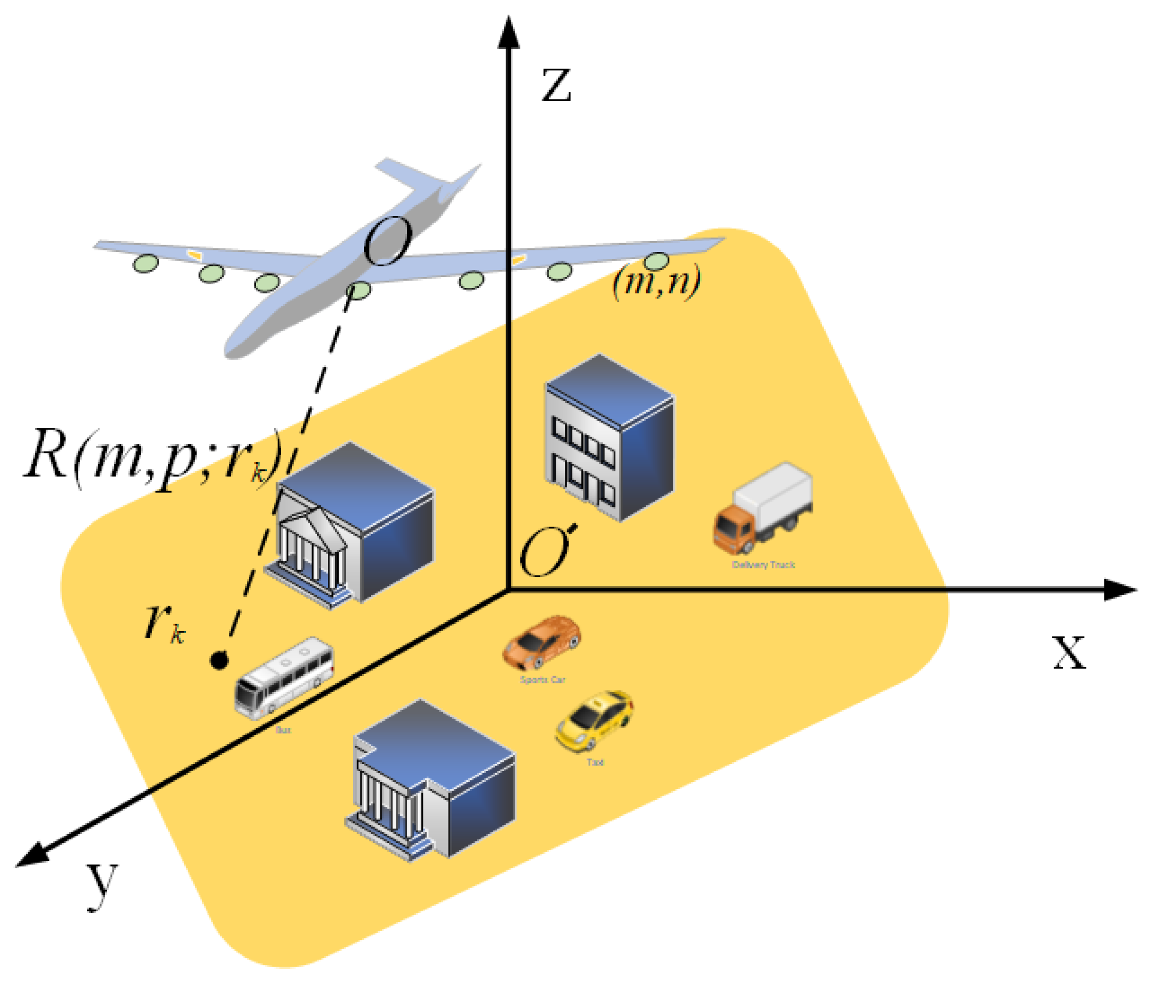
Figure 1 presents the array SAR system. A rectangular coordinate system represents the geometric relationship of imaging. The target scene coordinate system is established with the center of target scene O’ as the coordinate origin. The observation scene coordinate system is established with O as the coordinate origin. The z-direction is the elevation direction, the x-direction is the cross-track direction, and the y-direction is the along-track direction [32]. In this paper, the transmitting signal of the imaging system is a stepped-frequency (SF) signal.

The expression of the SF signal is as follows:

$s\left(t\right)={\displaystyle \sum _{n=1}^{N-1}}u(t-n{T}_1)e^{j2\pi f_{n}t}$ where $f_n=f_0+n\Delta f$ is the temporal frequency, $n=0,1,2,\cdots ,N-1$, $\Delta f$ is the increment of the temporal frequency, $N=\frac{{\mathrm{B}}_w}{\Delta f}$, $f_0$ is the start temporal frequency, and ${\mathrm{B}}_w$ denotes the bandwidth of the signal. $u(t-n{T}_1)$ can be expressed as

$$u(t-n{T}_1)=\left\{\begin{array}{cc}1,& 0<t-n{T}_1<T_2;\\ 0,& otherwise;\end{array}\right.$$

(1)

where $T_2$ is pulse width, and $T_1$ is the pulse repetition period.

The transmitted signal enters the free space through the transmitting antenna and interacts with the scattering point of the target to generate the scattered electromagnetic wave. After the receiving antenna receives the transmitted signal, the echo signal of the scattering point ${\mathbf{r}}_k$ at the antenna position $\left(m,p\right)$ is obtained.

$$s_r\left(l,m,p\right)=\sum _{n=1}^{N-1}\delta \left({\mathbf{r}}_k\right)u\left(t\left(l\right)-n{T}_1-\tau \left(m,p;{\mathbf{r}}_k\right)\right)e^{j2\pi f_n\left[t\left(l\right)-\tau \left(m,p;{\mathbf{r}}_k\right)\right]},$$

(2)

where $\delta \left({\mathbf{r}}_k\right)$ is the scattering coefficient of the scattering point ${\mathbf{r}}_k$.

The sampling number in the elevation, along-track and cross-track directions of an echo signal are L, M, and P, respectively. After discretizing the imaging space, $N_x$, $N_y$, and $N_z$ become the grid numbers of the whole scene in the range, azimuth, and elevation directions, respectively. The total number of 3D discrete imaging space grids is $M_s=N_x·N_y·N_z$. According to scattering center theory [5], 3D SAR imaging can be regarded as a linear observation system. Hence, the echo of the whole scene at the antenna position $\left(m,p\right)$ can be expressed as the linear superposition of the echo of all scattering points in the imaging scene.

$$s\left(l,m,p\right)=\sum _{k=1}^{M_s}\delta \left({\mathbf{r}}_k\right)\sum _{n=1}^{N-1}u\left(t\left(l\right)-n{T}_1-\tau \left(m,p;{\mathbf{r}}_k\right)\right)e^{j2\pi f_n\left[t\left(l\right)-\tau \left(m,p;{\mathbf{r}}_k\right)\right]}$$

(3)

$$1\le l\le L,1\le m\le M,1\le p\le P,1\le k\le M_s,$$

(4)

where $\tau \left(m,p;{\mathbf{r}}_k\right)$ is the time delay from scattering point ${\mathbf{r}}_k$ to array element $\left(m,p\right)$.

2.2. The Observation-Matrix-Based Sparse SAR Reconstruction Model

Let vector ${\mathbf{x}}_s\in C^{M_s\times 1}$ be the scattering coefficient vector of all the grid cells in the 3D imaging space:

$${\mathbf{x}}_s=\left\{\delta \left({\mathbf{r}}_k\right)\right\},k=1,2,···,M_s.$$

(5)

The time delay phase measurement vector ${\mathbf{a}}_s\left(l,m,p\right)\in C^{M_s\times 1}$ corresponding to the echo $s\left(l,m,p\right)$ is

$${\mathbf{a}}_s\left(l,m,p\right)=\left\{exp\left(j2\pi f_n\left[t\left(l\right)-\tau \left(m,p;{\mathbf{r}}_k\right)\right]\right)\right\}.$$

(6)

Thus, the echo signal can be expressed as the vector form

$$s\left(l,m,p\right)={\mathbf{a}}_s{\left(l,m,p\right)}^T{\mathbf{x}}_s.$$

(7)

The vector form of all echoes of linear array SAR is

$$\mathbf{y}=\left\{s\left(l,m,p\right)\right\},l=1,2,···,L,m=1,2,···,M,p=1,2,···,P.$$

(8)

The sparse SAR imaging model based on fully sampled raw data can be expressed as

$$\mathbf{y}=\mathbf{Ax}+{\mathbf{n}}_s,$$

(9)

where $\mathbf{A}$ is the measurement matrix of the 3D SAR echo, and ${\mathbf{n}}_s$ is the noise vector. After downsampling the echo data, the imaging model can be expressed as

$${\mathbf{y}}_D={\mathbf{A}}_D\mathbf{y}={\mathbf{A}}_D\mathbf{Ax}+{\mathbf{n}}_s=\mathbf{Rx}+{\mathbf{n}}_s,$$

(10)

where ${\mathbf{A}}_D$ is the downsampling matrix, and $\mathbf{R}$ is the SAR imaging measurement matrix.

According to the model in (10), the sparse reconstruction of the observation scene is acquired by solving the complex $L_q$ ($0\le q\le 1$) norm-regularization problem of (11)

$${\mathbf{y}}_{Ss}=\underset{\mathbf{x}}{min}\left\{{∥{\mathbf{y}}_D-\mathbf{Rx}∥}_2^2+\lambda {∥\mathbf{x}∥}_q^q\right\},$$

(11)

where $\lambda$ represents the regularization parameter.

2.3. Sparse Reconstruction Combining MM and Regularization

The optimization problem (11) is challenging to solve and has a high computational cost. Therefore, we use the MM framework to construct a surrogate function [27]. If we let $f\left(\mathbf{x}\right)={∥{\mathbf{y}}_D-\mathbf{Rx}∥}^2$, the surrogate function is as follows:

$$\stackrel{⌢}{f}(\mathbf{x},{\mathbf{x}}^{i-1})=f({\mathbf{x}}^{i-1})+\langle \mathbf{x}-{\mathbf{x}}^{i-1},\nabla f\left({\mathbf{x}}^{i-1}\right)\rangle +(1/2\mu ){\parallel \mathbf{x}-{\mathbf{x}}^{i-1}\parallel }_2^2+\lambda {∥\mathbf{x}∥}_q^q,$$

(12)

where $\mu \in \left(0,1/L\right)$ is step size, $\lambda >0$ is regularization parameters, and L is the Lipschitz constant of the gradient $\nabla f$.

For any $\mathbf{x}$, the surrogate function meets the following conditions:

$$\begin{array}{l}\stackrel{⌢}{f}\left(\mathbf{x},{\mathbf{x}}^{i-1}\right)\ge f\left(\mathbf{x}\right)\\ \stackrel{⌢}{f}\left({\mathbf{x}}^{i-1},{\mathbf{x}}^{i-1}\right)=f\left({\mathbf{x}}^{i-1}\right)\end{array}$$

(13)

Then, we update $\mathbf{x}$ in the minimization step ${\mathbf{x}}^i\in argmin\stackrel{⌢}{f}(\mathbf{x})$, and we can obtain the following relationship:

$$\begin{array}{c}\hfill f({\mathbf{x}}^i)\le \stackrel{⌢}{f}\end{array}\left({\mathbf{x}}^i,{\mathbf{x}}^{i-1}\right)\le \stackrel{⌢}{f}\left({\mathbf{x}}^{i-1},{\mathbf{x}}^{i-1}\right)=f({\mathbf{x}}^{i-1})$$

(14)

By simplifying the surrogate function and ignoring the constant term, (15) is obtained

$$\stackrel{⌢}{f}(\mathbf{x},{\mathbf{x}}^{i-1})=(1/2\mu ){\parallel \mathbf{x}-({\mathbf{x}}^{i-1}-\mu \nabla f({\mathbf{x}}^{i-1}))\parallel }_2^2+\lambda {∥\mathbf{x}∥}_q^q.$$

(15)

For different regularizations, different proximal regularization operators are used to obtain ${\mathbf{x}}^i$:

$${\mathbf{y}}_{Ss}={\mathbf{x}}^i={\tau }_q\left({\mathbf{x}}^{i-1}-\mu \nabla f\left({\mathbf{x}}^{i-1}\right);\mu {\lambda }^{\left(i\right)}\right),$$

(16)

where ${\tau }_q\left(;\right)$ is the proximal regularization operator, which is described in detail in Section 3.

3. The Sparse Reconstruction Method Combining MM and ${\mathit{L}}_{\mathit{q}}$ Regularization

In this section, we introduce the proposed sparse reconstruction method based on MM and $L_q$ regularization. First, we introduce MM-$L_1$. Then, due to the fact taht $L_1$ regularization often introduces extra bias in estimations [31], MM-$L_{1/2}$ is introduced. Next, MM-$L_0$ is presented. Finally, GMM-$L_q$ is also presented.

3.1. The Sparse Reconstruction Method Combining MM and $L_1$ Regularization

The $L_1$ regularization problem can be seen as being equivalent to the convex quadratic optimization problem, so it can be very effectively solved. $L_1$ regularization is widely used to solve the sparsity problem [28]. Therefore, we derived 3D sparse SAR imaging methods combining MM framework and $L_1$ regularization.

The full sampling SAR imaging model based on the image matrix operation can be expressed as [30]

$$\mathbf{Y}=\mathbf{WX}+\mathrm{N},$$

(17)

where $\mathbf{Y}$ is the echo data matrix, $\mathbf{W}$ is the system observation matrix, $\mathbf{X}$ is the backscattering coefficient matrix of the observation scene, and $\mathrm{N}$ is the noise matrix. After downsampling the echo data, the imaging model can be expressed as

$${\mathbf{Y}}_D=\mathbf{GY}=\mathbf{GWX}+\mathrm{N}=\mathrm{H}\mathbf{X}+\mathrm{N},$$

(18)

where $\mathbf{G}$ is the downsampling matrix, $\mathrm{H}$ is the SAR imaging measurement matrix, and $\mathrm{N}$ is the noise matrix.

For the model of (18), the reconstruction of the observation scene can be obtained by solving (19):

$${\mathbf{Y}}_{Sp}=\underset{\mathbf{X}}{min}\left\{{∥{\mathbf{Y}}_D-\mathrm{H}\mathbf{X}∥}_F^2+\lambda {∥\mathbf{X}∥}_1\right\},$$

(19)

where ${\mathbf{Y}}_{Sp}$ is the reconstructed backscattered coefficient of $\mathbf{X}$, ${∥·∥}_F$ is the Frobenius norm of a matrix, and $\lambda$ represents the regularization parameter. However, the observation matrix $\mathrm{H}$ cannot be directly constructed because of the range-array coupling of echo data. The method introduced in Section 2.2 is an alternative, but its computational complexity is huge for 3D scene reconstructions. Therefore, we define the inverse of MF imaging procedure as $\mathrm{T}\left(·\right)={\mathrm{M}}^{-1}\left(·\right)$.

If we let $\mathrm{M}\left(·\right)$ denote the MF imaging process, then:

$${\mathbf{Y}}_{MF}=\mathrm{M}\left({\mathbf{Y}}_D\right)=\mathrm{M}\left(\mathbf{HX}\right),$$

(20)

where ${\mathbf{Y}}_{MF}$ represents the complex image data based on MF, and $\mathbf{X}$ represents the scattering distribution of the observation scene, ${\mathbf{Y}}_{MF}$ is always the approximate value of $\mathbf{X}$ due to the existence of sidelobe and noise, and $\mathrm{M}\mathbf{H}\approx \mathbf{I}$ [28].

$$\mathrm{T}\left(\mathbf{X}\right)={\mathrm{M}}^{-1}\left(\mathbf{X}\right)\approx \mathrm{H}\mathbf{X}$$

(21)

After MF processing (18), we obtain

$$\begin{array}{c}\mathrm{M}\left(\mathbf{Y}\right)\approx \mathrm{M}\left(\mathrm{T}\left(\mathbf{X}\right)\right)+\mathrm{M}\left(\mathrm{N}\right)\hfill \\ {\mathbf{Y}}_{MF}\approx \mathbf{X}+{\mathrm{N}}_M.\hfill \end{array}$$

(22)

After that, we can reconstruct the imaging by solving (23)

$${\mathbf{Y}}_{SR}=\underset{\mathbf{X}}{min}\left\{{∥{\mathbf{Y}}_{\mathrm{MF}}-\mathbf{X}∥}_F^2+\lambda {∥\mathbf{X}∥}_1\right\},$$

(23)

where ${\mathbf{Y}}_{SR}$ is the recovery result of $\mathbf{X}$, and ${∥·∥}_F$ is the Frobenius norm of a matrix.

If we let $F\left(\mathbf{X}\right)={∥{\mathbf{Y}}_{\mathrm{MF}}-\mathbf{X}∥}_F^2$; we can then construct the surrogate function using the MM idea for question (23).

$$\stackrel{⌢}{F}\left({\mathbf{X}}^{i-1},{\mathbf{X}}^{i-1}\right)=\left(1/2\mu \right){∥\mathbf{X}-\left({\mathbf{X}}^{i-1}-\mu \nabla F({\mathbf{X}}^{i-1})\right)∥}_F^2+\lambda {∥\mathbf{X}∥}_1$$

(24)

The imaging scene is reconstructed by solving the following optimization problem:

$${\mathbf{Y}}_{SR}=\underset{\mathbf{X}}{min}\left\{\left(1/2\mu \right){∥\mathbf{X}-\left({\mathbf{X}}^{i-1}-\mu \nabla F({\mathbf{X}}^{i-1})\right)∥}_F^2+\lambda {∥\mathbf{X}∥}_1\right\}.$$

(25)

The proximal operator for L1 regularization is used to solve (24):

$${\mathbf{Y}}_{SR}={\mathbf{X}}^i={\tau }_1\left({\mathbf{X}}^{i-1}-\mu \nabla F\left({\mathbf{X}}^{i-1}\right);\mu {\lambda }^{\left(i\right)}\right),$$

(26)

where ${\tau }_1\left(;\right)$ is the proximal regular operator for $L_1$ regularization.

The procedure of MM-$L_1$ is shown in Algorithm 1, which is used to solve the optimization problem of (25) to obtain the reconstructed 3D SAR image.

${\left|{\mathbf{Y}}_{SS}^{\left(i\right)}\right|}_{k+1}$ is the (k + 1)th largest amplitude element of image $\left|{\mathbf{Y}}_{SS}^{\left(i\right)}\right|$, $\mu$ is the step size, the parameter k denotes the scene sparsity, and ${\tau }_1\left({\mathbf{Y}}_{SS}^{\left(i\right)};\mu {\lambda }^{\left(i\right)}\right)$ is the proximal regular operator for $L_1$ regularization, which is defined as follows

$${\tau }_1\left({\mathbf{Y}}_{SS}^{\left(i\right)};\mu {\lambda }^{\left(i\right)}\right)=sign({\mathbf{Y}}_{SS}^{\left(i\right)})max(\left|{\mathbf{Y}}_{SS}^{\left(i\right)}\right|-\mu {\lambda }^{\left(i\right)},0).$$

(27)

3.2. Sparse Reconstruction Method Combining MM and $L_{1/2}$ Regularization

When $q=1/2$, the sparse reconstruction of the scene is realized by solving (28):

$${\mathbf{Y}}_{SR}=\underset{\mathbf{X}}{min}\left\{{∥{\mathbf{Y}}_{MF}-\mathbf{X}∥}_F^2+\lambda {∥\mathbf{X}∥}_{1/2}^{1/2}\right\}.$$

(28)

We reconstructed the scene through the surrogate function and proximal regular operator for $L_{1/2}$ regularization [31]. The surrogate function was as follows:

$$\stackrel{⌢}{F}\left(\mathbf{X},{\mathbf{X}}^{i-1}\right)=\left(1/2\mu \right){∥\mathbf{X}-\left({\mathbf{X}}^{i-1}-\mu \nabla F({\mathbf{X}}^{i-1})\right)∥}_F^2+\lambda {∥\mathbf{X}∥}_{1/2}^{1/2}$$

(29)

Algorithm 1 The procedure of MM-$L_1$

Input: 3D complex image data ${\mathbf{Y}}_{MF}$; Error parameter $\epsilon$; Step size $\mu$; Maximum number of iterations $I_{max}$; Reconstruction image ${\mathbf{Y}}_S^{\left(0\right)}=\mathbf{0}$.            While $1\le i\le I_{max}$ and $\mathrm{Rs}>\epsilon$ do                        $t^{\left(i\right)}=0.5\left(1+\sqrt{1+4{t^{\left(i-1\right)}}^2}\right)$                        ${\mathbf{Y}}_{SS}^{\left(i\right)}=\mu {\mathbf{Q}}^{(i-1)}+{\mathbf{Y}}_S^{(i-1)}+\frac{t^{(i-1)}-1}{t^{\left(i\right)}}\left({\mathbf{Y}}_S^{(i-1)}-{\mathbf{Y}}_S^{(i-2)}\right)$                        ${\lambda }^{\left(i\right)}={\left|{\mathbf{Y}}_{SS}^{\left(i\right)}\right|}_{k+1}/\mu$                        ${\mathbf{Q}}^{\left(i\right)}={\mathbf{Y}}_{MF}-{\mathbf{Y}}_S^{(i-1)}$                        ${\mathbf{Y}}_S^{\left(i\right)}={\tau }_1\left({\mathbf{Y}}_{SS}^{\left(i\right)};\mu {\lambda }^{\left(i\right)}\right)$                        $Rs={∥{\mathbf{Y}}_S^{\left(i\right)}-{\mathbf{Y}}_S^{(i-1)}∥}_F$                        $\mu =\mu /2$                        $i=i+1$            End While Output: Sparse reconstruction image without PI reservation ${\mathbf{Y}}_{SR}={\mathbf{Y}}_S^{\left(i\right)}$; Sparse reconstruction image with PI preserved ${\mathbf{Y}}_{SS}={\mathbf{Y}}_{SS}^{\left(i\right)}$.

After this, the imaging scene was reconstructed by solving the following optimization problem:

$${\mathbf{Y}}_{SR}=\underset{\mathbf{X}}{min}\left\{\left(1/2\mu \right){∥\mathbf{X}-\left({\mathbf{X}}^{i-1}-\mu \nabla F({\mathbf{X}}^{i-1})\right)∥}_F^2+\lambda {∥\mathbf{X}∥}_{1/2}\right\}.$$

(30)

The proximal operator is used to solve (30):

$${\mathbf{Y}}_{SR}={\mathbf{X}}^i={\tau }_{1/2}\left({\mathbf{X}}^{i-1}-\mu \nabla F\left({\mathbf{X}}^{i-1}\right);\mu {\lambda }^{\left(i\right)}\right),$$

(31)

where ${\tau }_{1/2}\left(;\right)$ is the proximal regular operator for $L_{1/2}$ regularization.

To effectively and efficiently obtain 3D images, we adopted the MM-$L_{1/2}$ algorithm. The detailed procedure of MM-$L_{1/2}$ is shown in Algorithm 2.

${\tau }_{1/2}\left({\mathbf{Y}}_{SS}^{\left(i\right)};\mu {\lambda }^{\left(i\right)}\right)$ is defined as follows:

$${\tau }_{1/2}\left({\mathbf{Y}}_{SS}^{\left(i\right)};\mu {\lambda }^{\left(i\right)}\right)=\left\{\begin{array}{cc}g\left({\mathbf{Y}}_{SS}^{\left(i\right)};\mu {\lambda }^{\left(i\right)}\right),& \left|{\mathbf{Y}}_{SS}^{\left(i\right)}\right|>{\left(54\right)}^{1/3}{\left(\mu {\lambda }^{\left(i\right)}\right)}^{2/3}/4\\ 0,& otherwise,\end{array}\right.$$

(32)

where $g\left({\mathbf{Y}}_{SS}^{\left(i\right)};\mu {\lambda }^{\left(i\right)}\right)$ is defined as follows:

$$g\left({\mathbf{Y}}_{SS}^{\left(i\right)};\mu {\lambda }^{\left(i\right)}\right)=\frac{2}{3}{\mathbf{Y}}_{SS}^{\left(i\right)}\left\{1+cos\left[\frac{2\pi }{3}-\frac{2}{3}arccos\left(\frac{{\lambda }^{\left(i\right)}\mu }{8}{\left(\frac{\left|{\mathbf{Y}}_{SS}^{\left(i\right)}\right|}{3}\right)}^{-\frac{3}{2}}\right)\right]\right\}$$

(33)

Algorithm 2 The procedure of MM-$L_{1/2}$

Input: 3D complex image data ${\mathbf{Y}}_{MF}$; Error parameter $\epsilon$; Step size $\mu$; Maximum number of iterations $I_{max}$; Reconstruction image ${\mathbf{Y}}_S^{\left(0\right)}=\mathbf{0}$.             While $1\le i\le I_{max}$ and $\mathrm{Rs}>\epsilon$ do                        $t^{\left(i\right)}=0.5\left(1+\sqrt{1+4{t^{\left(i-1\right)}}^2}\right)$                        ${\mathbf{Y}}_{SS}^{\left(i\right)}=\mu {\mathbf{Q}}^{(i-1)}+{\mathbf{Y}}_S^{(i-1)}+\frac{t^{(i-1)}-1}{t^{\left(i\right)}}\left({\mathbf{Y}}_S^{(i-1)}-{\mathbf{Y}}_S^{(i-2)}\right)$                        ${\lambda }^{\left(i\right)}=\sqrt{96}{\left({\left|{\mathbf{Y}}_{SS}^{\left(i\right)}\right|}_{k+1}\right)}^{3/2}/9\mu$                        ${\mathbf{Q}}^{\left(i\right)}={\mathbf{Y}}_{MF}-{\mathbf{Y}}_S^{(i-1)}$                        ${\mathbf{Y}}_S^{\left(i\right)}={\tau }_{1/2}\left({\mathbf{Y}}_{SS}^{\left(i\right)};\mu {\lambda }^{\left(i\right)}\right)$                        $Rs={∥{\mathbf{Y}}_S^{\left(i\right)}-{\mathbf{Y}}_S^{(i-1)}∥}_F$                        $\mu =\mu /2$                        $i=i+1$             End While Output: Sparse reconstruction image without PI reservation ${\mathbf{Y}}_{SR}={\mathbf{Y}}_S^{\left(i\right)}$; Sparse reconstruction image with PI preserved ${\mathbf{Y}}_{SS}={\mathbf{Y}}_{SS}^{\left(i\right)}$.

3.3. Sparse Reconstruction Method Combining MM and $L_0$ Regularization

When q is 0, the sparse reconstruction of the scene is realized by solving (34):

$${\mathbf{Y}}_{SR}=\underset{\mathbf{X}}{min}\left\{{∥{\mathbf{Y}}_{MF}-\mathbf{X}∥}_F^2+\lambda {∥\mathbf{X}∥}_0^{}\right\}.$$

(34)

The surrogate function and proximal regular operator for $L_0$ regularization were used to reconstruct the scene. The surrogate function was as follows:

$$\stackrel{⌢}{F}\left(\mathbf{X},{\mathbf{X}}^{i-1}\right)=\left(1/2\mu \right){∥\mathbf{X}-\left({\mathbf{X}}^{i-1}-\mu \nabla F({\mathbf{X}}^{i-1})\right)∥}_F^2+\lambda {∥\mathbf{X}∥}_0$$

(35)

Then, the imaging scene was reconstructed by solving the following optimization problem:

$${\mathbf{Y}}_{SR}=\underset{\mathbf{X}}{min}\left\{\left(1/2\mu \right){∥\mathbf{X}-\left({\mathbf{X}}^{i-1}-\mu \nabla F\left({\mathbf{X}}^{i-1}\right)\right)∥}_F^2+\lambda {∥\mathbf{X}∥}_0\right\}.$$

(36)

The proximal operator was used to solve (36):

$${\mathbf{Y}}_{SR}={\mathbf{X}}^i={\tau }_0\left({\mathbf{X}}^{i-1}-\mu \nabla F\left({\mathbf{X}}^{i-1}\right);\mu {\lambda }^{\left(i\right)}\right),$$

(37)

where ${\tau }_0\left(;\right)$ is the proximal regular operator for $L_0$ regularization.

The detailed procedure of MM-$L_0$ is shown in Algorithm 3.

The proximal regular operator for $L_0$ regularization ${\tau }_0\left({\mathbf{Y}}_{SS}^{\left(i\right)};\mu {\lambda }^{\left(i\right)}\right)$ is defined as follows:

$${\tau }_0\left({\mathbf{Y}}_{SS}^{\left(i\right)};\mu {\lambda }^{\left(i\right)}\right)=\left\{\begin{array}{cc}sign\left({\mathbf{Y}}_{SS}^{\left(i\right)}\right)\left|{\mathbf{Y}}_{SS}^{\left(i\right)}\right|,& {\mathbf{Y}}_{SS}^{\left(i\right)}>\mu {\lambda }^{\left(i\right)}\\ 0,& otherwise\end{array}\right.$$

(38)

Algorithm 3 The procedure of MM-$L_0$

Input: 3D complex image data ${\mathbf{Y}}_{MF}$; Error parameter $\epsilon$; Step size $\mu$; Maximum number of iterations $I_{max}$; Reconstruction image ${\mathbf{Y}}_S^{\left(0\right)}=\mathbf{0}$.             While $1\le i\le I_{max}$ and $\mathrm{Rs}>\epsilon$ do                        ${\mathbf{Y}}_{SS}^{\left(i\right)}=\mu {\mathbf{Q}}^{(i-1)}+{\mathbf{Y}}_S^{(i-1)}$                        ${\lambda }^{\left(i\right)}={\left|{\mathbf{Y}}_{SS}^{\left(i\right)}\right|}_{k+1}/\mu$                        ${\mathbf{Q}}^{\left(i\right)}={\mathbf{Y}}_{MF}-{\mathbf{Y}}_S^{(i-1)}$                        ${\mathbf{Y}}_S^{\left(i\right)}={\tau }_0\left({\mathbf{Y}}_{SS}^{\left(i\right)};\mu {\lambda }^{\left(i\right)}\right)$                        $Rs={∥{\mathbf{Y}}_S^{\left(i\right)}-{\mathbf{Y}}_S^{(i-1)}∥}_F$                        $\mu =\mu /2$                        $i=i+1$             End While Output: Sparse reconstruction image without PI reservation ${\mathbf{Y}}_{SR}={\mathbf{Y}}_S^{\left(i\right)}$; Sparse reconstruction image with PI preserved ${\mathbf{Y}}_{SS}={\mathbf{Y}}_{SS}^{\left(i\right)}$.

3.4. Generalized MM-$L_q$ ($0\le q\le 1$) Method

In this subsection, we illustrate a generalized MM-$L_q$ ($0\le q\le 1$) algorithm via combining MM and the generalized proximal regular operator. The surrogate function for $L_q$ was as follows:

$$\stackrel{⌢}{F}\left(\mathbf{X},{\mathbf{X}}^{i-1}\right)=\left(1/2\mu \right){∥\mathbf{X}-\left({\mathbf{X}}^{i-1}-\mu \nabla F({\mathbf{X}}^{i-1})\right)∥}_F^2+\lambda {∥\mathbf{X}∥}_q^q$$

(39)

The proximal operator for $L_q$ was used to reconstruct the imaging scene:

$${\mathbf{Y}}_{SR}={\mathbf{X}}^i={\tau }_{Gq}\left({\mathbf{X}}^{i-1}-\mu \nabla F\left({\mathbf{X}}^{i-1}\right);\mu {\lambda }^{\left(i\right)}\right).$$

(40)

Then, we provided a concise derivation of $Th$. Let x and y be elements of matrices $\mathbf{X}$ and ${\mathbf{Y}}_{SS}$, respectively.

$$v\left(x\right)=\frac{1}{2}{\left(x-y\right)}^2+\lambda {\left|x\right|}^q.$$

(41)

The first and second derivatives of $v\left(x\right)$ are as follows:

$$\begin{array}{c}\hfill v^{\prime }\left(x\right)=x-y+\lambda q{x}^{q-1}\\ \hfill v^{″}\left(x\right)=1+\lambda q(q-1)x^{q-2}\end{array}$$

(42)

Let $v^{{}^{″}}\left(x^{{}^{″}}\right)=0$,

$$x^{{}^{″}}={\left[\lambda \left(1-q\right)\right]}^{1/\left(2-q\right)}.$$

(43)

So $v\left(x\right)$ is convex in the range of $\left(x^{{}^{″}},+\infty \right)$. Thus, we obtained $Th$ and its corresponding $x_q$ via solving the nonlinear equation [24]:

$$\frac{1}{2}{\left(x_q-Th\left(\lambda \right)\right)}^2+\lambda {\left(x_q\right)}^q=\frac{1}{2}{\left(Th\left(\lambda \right)\right)}^2$$

(44)

$$x_q-Th\left(\lambda \right)+\lambda q{\left(x_q\right)}^{q-1}=0,$$

(45)

We substituted (45) into (44) to obtain the following relationship:

$${\left(x_q\right)}^q\left(2\lambda \left(1-q\right)-{\left(x_q\right)}^{2-q}\right)=0.$$

(46)

Thus, in the range of $\left(x^{{}^{″}},+\infty \right)$, the unique solution is as follows:

$$x_q={\left(2\lambda \left(1-q\right)\right)}^{1/(2-q)},$$

(47)

and $Th$ is

$$Th\left(\lambda \right)={\left[2\lambda \left(1-q\right)\right]}^{1/\left(2-q\right)}+\lambda q{\left[2\lambda \left(1-q\right)\right]}^{\left(q-1\right)/(2-q)},$$

(48)

The generalized proximal regularization operator is as following Algorithm 4:

Algorithm 4 The generalized proximal regularization operator

Input: q; $\lambda$; ${\mathbf{Y}}_{SS}^{}$.             $Th={\left[2\lambda \left(1-q\right)\right]}^{1/\left(2-q\right)}+\lambda q{\left[2\lambda \left(1-q\right)\right]}^{\left(q-1\right)/(2-q)}$             If $\left|{\mathbf{Y}}_{SS}^{}\right|\le Th$                            ${\tau }_{Gq}\left({\mathbf{Y}}_{SS}^{};\mu \lambda \right)=0$             Else $j=0,{\mathbf{Y}}_{Gq}^{\left(j\right)}=\left|{\mathbf{Y}}_{SS}^{}\right|$                            Iterate on $j=0,1,2$                               ${\mathbf{Y}}_{Gq}^{(j+1)}=\left|{\mathbf{Y}}_{SS}^{}\right|-\lambda q{\left({\mathbf{Y}}_{Gq}^{\left(j\right)}\right)}^{q-1}$                               $j=j+1$                            ${\tau }_{Gq}\left({\mathbf{Y}}_{SS}^{};\mu \lambda \right)=sign\left({\mathbf{Y}}_{SS}^{}\right){\mathbf{Y}}_{Gq}^{\left(j\right)}$             End If Output: ${\tau }_{Gq}\left({\mathbf{Y}}_{SS}^{};\mu {\lambda }^{}\right)$.

The detailed procedure of GMM-$L_q$ is shown in Algorithm 5 for solving $L_q$ ($0\le q\le 1$) regularization problems.

Algorithm 5 The procedure of GMM-$L_q$

Input: 3D complex image data ${\mathbf{Y}}_{MF}$; Error parameter $\epsilon$; Step size $\mu$; Maximum number of iterations $I_{max}$; Reconstruction image ${\mathbf{Y}}_S^{\left(0\right)}=\mathbf{0}$.             While $1\le i\le I_{max}$ and $\mathrm{Rs}>\epsilon$ do                        $t^{\left(i\right)}=0.5\left(1+\sqrt{1+4{t^{\left(i-1\right)}}^2}\right)$                        ${\mathbf{Y}}_{SS}^{\left(i\right)}=\mu {\mathbf{Q}}^{(i-1)}+{\mathbf{Y}}_S^{(i-1)}+\frac{t^{(i-1)}-1}{t^{\left(i\right)}}\left({\mathbf{Y}}_S^{(i-1)}-{\mathbf{Y}}_S^{(i-2)}\right)$                        ${\lambda }^{\left(i\right)}={\left|{\mathbf{Y}}_{SS}^{\left(i\right)}\right|}_{k+1}/\mu$                        ${\mathbf{Q}}^{\left(i\right)}={\mathbf{Y}}_{MF}-{\mathbf{Y}}_S^{(i-1)}$                        ${\mathbf{Y}}_S^{\left(i\right)}={\tau }_{Gq}\left({\mathbf{Y}}_{SS}^{\left(i\right)};\mu {\lambda }^{\left(i\right)}\right)$                        $Rs={∥{\mathbf{Y}}_S^{\left(i\right)}-{\mathbf{Y}}_S^{(i-1)}∥}_F$                        $\mu =\mu /2$                        $i=i+1$             End While Output: Sparse reconstruction image without PI reservation ${\mathbf{Y}}_{SR}={\mathbf{Y}}_S^{\left(i\right)}$; Sparse reconstruction image with PI preserved ${\mathbf{Y}}_{SS}={\mathbf{Y}}_{SS}^{\left(i\right)}$.

4. Results and Analysis

In this section, several simulations and experiments are presented to verify the effectiveness of the proposed method. We used target-to-background ratio (TBR) and image entropy (ENT) [33] as the quantitative evaluation criteria to evaluate the effect of the sparse reconstruction algorithm. These are defined by:

$$\mathrm{TBR}=20\mathrm{lo}{\mathrm{g}}_{10}\left(\frac{{\mathrm{N}}_{\mathrm{B}}\sum _{({\mathrm{v}}_1,{\mathrm{v}}_2,{\mathrm{v}}_3)\in \mathrm{T}}{\left|\mathbf{Y}\right|}_{({\mathrm{v}}_1,{\mathrm{v}}_2,{\mathrm{v}}_3)}}{{\mathrm{N}}_{\mathrm{T}}\sum _{({\mathrm{v}}_1,{\mathrm{v}}_2,{\mathrm{v}}_3)\in \mathrm{B}}{\left|\mathbf{Y}\right|}_{({\mathrm{v}}_1,{\mathrm{v}}_2,{\mathrm{v}}_3)}}\right),$$

(49)

$$\mathrm{ENT}=-\sum _{h\left(i\right)}{p}_{i}log{p}_i,$$

(50)

where T and B are the set of targets and background points, respectively, ${\mathrm{N}}_{\mathrm{B}}$ is the number of pixels contained in the background, ${\mathrm{N}}_{\mathrm{T}}$ is the number of pixels contained in the target region, $p_i$ is the proportion of pixels with amplitude i in the image, and $h\left(i\right)$ is the total gray value of the image histogram. The larger the value of the TBR, the more obvious the noise suppression effect. The smaller the ENT value, the clearer the image.

Firstly, a combat-vehicle model was used for 3D simulation imaging. Then, to verify the noise suppression effect of algorithms in this paper, we added additive white Gaussian noise (AWGN) to the simulated echo data of aircraft and then reconstructed the scene using MF, MM-$L_1$, MM-$L_{1/2}$, MM-$L_0$, and GMM-$L_q$, respectively. Finally, two sets of real 3D ground-based array SAR data were used to verify the effectiveness of the algorithms. The real data of the complex scene was provided by [34]. The imaging model was a 3D linear array SAR.

4.1. Combat-Vehicle Model

The combat-vehicle model simulation was carried out without noise to verify the effect of sidelobe suppression. Simulation parameters were as follows. The center frequency was 37.5 GHz, the bandwidth was 163.8 MHz, the platform height was 1000 m, and the inear antenna array length was $3\times 3$ m. The dimensions of the 3D image matrix were $512\times 101\times 101$. We set q to 0.8 to verify the feasibility of GMM-$L_q$. The elevation, along-track and cross-track resolutions were 0.915 m, 1.333 m, and 1.333 m, respectively.

Figure 2 and Figure 3 show the imaging results of the MF, MM-$L_1$, MM-$L_{1/2}$, MM-$L_0$, and GMM-$L_{0.8}$ corresponding to the 100% and 75% sampling rates, respectively. It can be seen that the proposed algorithms improve the image quality and suppress the sidelobe.

The TBR values of the MF results and sparse imaging are listed in

Table 1. The TBR of the Combat Vehicle.

Sampling Rates	MF	MM-${\mathit{L}}_1$	MM-${\mathit{L}}_{1/2}$	MM-${\mathit{L}}_0$	GMM-${\mathit{L}}_{0.8}$
100%	32.2816	56.8821	58.1102	55.5013	57.2132
75%	28.7322	55.8019	56.2296	52.3123	56.1083

. The TBR of MF was 32.2816 dB and 28.7322 dB at sampling rates of 100% and 75%, respectively. When the sampling rate was 100%, the TBR of MM-$L_1$, MM-$L_{1/2}$, MM-$L_0$, and GMM-$L_{0.8}$ were 56.8821 dB, 58.1102 dB, 55.5013 dB, and 57.2132 dB, respectively. When the sampling rate was 75%, the TBR of MM-$L_1$, MM-$L_{1/2}$, MM-$L_0$, and GMM-$L_{0.8}$ were 55.8019 dB, 56.2296 dB, 52.3123 dB, and 56.1083 dB, respectively. Compared with MF, the MM-$L_1$, MM-$L_{1/2}$, MM-$L_0$,and GMM-$L_{0.8}$ suppress the sidelobe effectively with a TBR value that increased by approximately 25 dB. The ENT values of the MF results and sparse imaging are listed in

Table 2. The ENT of the Combat Vehicle.

Sampling Rates	MF	MM-${\mathit{L}}_1$	MM-${\mathit{L}}_{1/2}$	MM-${\mathit{L}}_0$	GMM-${\mathit{L}}_{0.8}$
100%	2.1957	0.1123	0.0616	0.1231	0.0976
75%	2.9766	0.1345	0.0867	0.1401	0.1205

. For full sampling, the ENT of MF was 2.1957 while those of MM-$L_1$, MM-$L_{1/2}$, MM-$L_0$, and GMM-$L_{0.8}$ were 0.1123, 0.0616, 0.1231, and 0.0976, respectively. When the sampling rate was 75%, the ENT of MF was 2.9766, while those of MM-$L_1$, MM-$L_{1/2}$, MM-$L_0$, and GMM-$L_{0.8}$ were 0.1345, 0.0867, 0.1401, and 0.1205, respectively. Compared with the ENT of MF, the ENT of MM-$L_1$, MM-$L_{1/2}$, MM-$L_0$, and GMM-$L_{0.8}$ decreased by approximately 2, which shows that the reconstructed image quality of the proposed methods improved.

4.2. 3D Aircraft Imaging with AWGN

The aircraft modeled using AWGN was used to verify the effectiveness of the proposed method in a complex environment. The simulation parameters were as follows. The center frequency was 37.5 GHz, the bandwidth was 163.8 MHz, the platform height was 1000 m, and the linear antenna array length was $3\times 3$ m. The dimension of image matrix was $512\times 101\times 101$

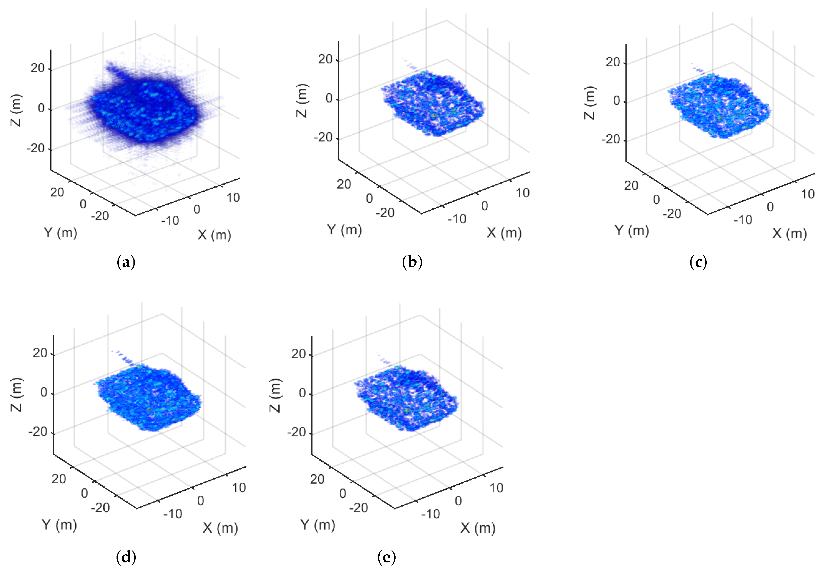
The elevation, along-track and cross-track resolutions were 0.915 m, 1.333 m, and 1.333 m, respectively. Figure 4 shows the imaging results of MF, MM-$L_1$, MM-$L_{1/2}$, MM-$L_0$, and GMM-$L_{0.8}$ with AWGN on the simulated echo data at 100%. Figure 5 shows the imaging results of MF, MM-$L_1$, MM-$L_{1/2}$, MM-$L_0$, and GMM-$L_{0.8}$ with AWGN on the simulated echo data at 75%. Compared with MF, using MM-$L_1$, MM-$L_{1/2}$, MM-$L_0$, and GMM-$L_{0.8}$ can efficiently suppress noise and improve the imaging results of the aircraft. Quantitative analysis with TBR is listed in

Table 3. The TBR of the Aircraft.

Sampling Rates	MF	MM-${\mathit{L}}_1$	MM-${\mathit{L}}_{1/2}$	MM-${\mathit{L}}_0$	GMM-${\mathit{L}}_{0.8}$
100%	25.3125	55.1235	56.4503	53.5276	55.1685
75%	24.2586	54.2167	55.5226	53.0124	55.0645

. The ENT of different algorithms is listed in

Table 4. The ENT of the Aircraft.

Sampling Rates	MF	MM-${\mathit{L}}_1$	MM-${\mathit{L}}_{1/2}$	MM-${\mathit{L}}_0$	GMM-${\mathit{L}}_{0.8}$
100%	2.9295	0.1037	0.0853	0.1069	0.0988
75%	3.1164	0.1091	0.0866	0.1098	0.1084

.

When the sampling rate was 100%, the TBR of MF, MM-$L_1$, MM-$L_{1/2}$, MM-$L_0$, and GMM-$L_{0.8}$ were 25.3125 dB, 55.1235 dB, 56.4503 dB, 53.5276 dB, and 55.1685 dB, respectively. When the sampling rate was 75%, the TBR of MF, MM-$L_1$, MM-$L_{1/2}$, MM-$L_0$, and GMM-$L_{0.8}$ were 24.2586 dB, 54.2167 dB, 55.5226 dB, 53.0124 dB, and 55.0645 dB, respectively. Compared with the TBR of MF, the TBR of MM-$L_1$, MM-$L_{1/2}$, MM-$L_0$, and GMM-$L_{0.8}$ increased by approximately 30 dB. For full sampling, the ENT of MF was 2.9295, while those of MM-$L_1$, MM-$L_{1/2}$, MM-$L_0$, and GMM-$L_{0.8}$ were 0.1037, 0.0853, 0.1069, and 0.0988, respectively. When the sampling rate was 75%, the ENT of MF was 3.1164, while those of MM-$L_1$, MM-$L_{1/2}$, MM-$L_0$, and GMM-$L_{0.8}$ were 0.1091, 0.0866, 0.1098, and 0.1084, respectively. Compared with the ENT of MF, the TBR of MM-$L_1$, MM-$L_{1/2}$, MM-$L_0$, and GMM-$L_{0.8}$ decreased by approximately 3. The results show that the proposed algorithms effectively improve the quality of SAR images.

4.3. Experiments Based on Ground-Based Array SAR Data

A ground-based array SAR system was used to verify the effect of the proposed algorithms. System parameters were as follows. The carrier frequency was 10 GHz, the signal bandwidth was 2 GHz, and the array size was $1.5\times 1.5$ m. The range, along-track and cross-track resolutions were 0.075 m, 0.05 m, and 0.05 m, respectively.

The experimental scenario is shown in Figure 6a. We obtained the echo of the scene through the array SAR system and performed 3D imaging using MM, MM-$L_1$, MM-$L_{1/2}$, MM-$L_0$, and GMM-$L_{0.8}$. The imaging results of the different algorithms corresponding to the 100% and 75% sampling rates are shown in Figure 7 and Figure 8, respectively.

The results of the quantitative analysis with TBR are listed in

Table 5. The TBR of the Ground-Based Array SAR Data.

Sampling Rates	MF	MM-${\mathit{L}}_1$	MM-${\mathit{L}}_{1/2}$	MM-${\mathit{L}}_0$	GMM-${\mathit{L}}_{0.8}$
100%	33.0913	70.6076	72.0131	68.7402	71.2652
75%	31.5164	69.1123	71.0673	67.6913	70.5451

. When the sampling rate was 100%, the TBR of MM-$L_1$, MM-$L_{1/2}$, MM-$L_0$, and GMM-$L_{0.8}$ were 33.0913 dB, 70.6076 dB, 72.0131 dB, 68.7402 dB, and 71.2652 dB, respectively. When the sampling rate was 75%, the TBR of MF, MM-$L_1$, MM-$L_{1/2}$, MM-$L_0$, and GMM-$L_{0.8}$ were 31.5164 dB, 69.1123 dB, 71.0673 dB, 67.6913 dB, and 70.5451 dB, respectively. Compared with the TBR of MF, the TBR of the proposed algorithms increased significantly. The ENT values of the different algorithms are listed in

Table 6. The ENT of the Ground-Based Array SAR Data.

Sampling Rates	MF	MM-${\mathit{L}}_1$	MM-${\mathit{L}}_{1/2}$	MM-${\mathit{L}}_0$	GMM-${\mathit{L}}_{0.8}$
100%	2.6935	0.0398	0.0209	0.0419	0.0236
75%	2.9392	0.0403	0.0211	0.0422	0.0254

. For full sampling, the ENT of MF was 2.6935, while those of MM-$L_1$, MM-$L_{1/2}$, MM-$L_0$, and GMM-$L_{0.8}$ were 0.0398, 0.0209, 0.0419, and 0.0236, respectively. When the sampling rate was 75%, the ENT of MF was 2.9392, while those of MM-$L_1$, MM-$L_{1/2}$, MM-$L_0$, and GMM-$L_{0.8}$ were 0.0403, 0.0211, 0.0422, and 0.0254, respectively. The ENT of the proposed algorithms was much smaller than that of MF. Therefore, the image quality was effectively improved.

4.4. Real SAR Data of Complex Scenes

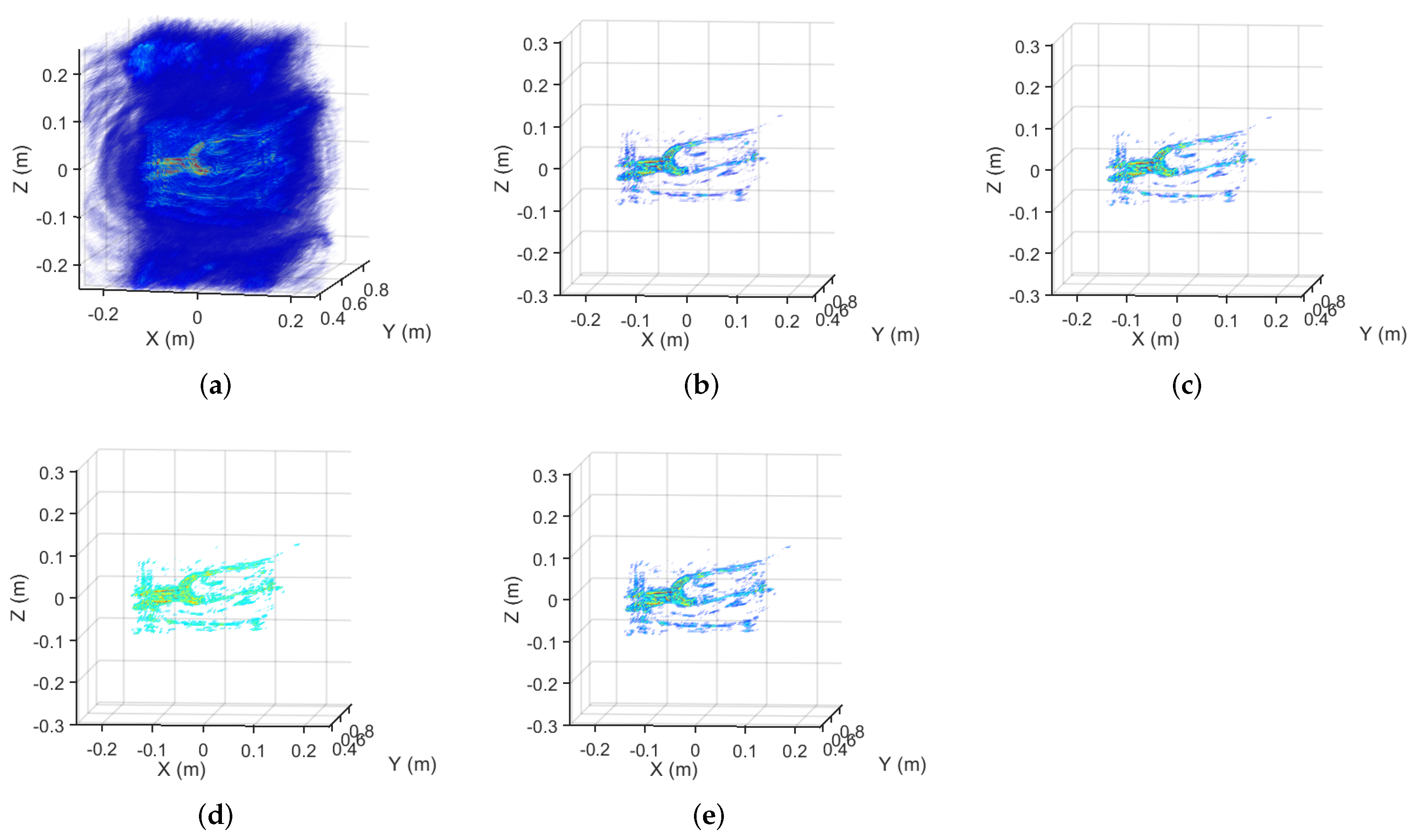
Another set of real data of complex scenes was used to verify the effectiveness and robustness of the proposed algorithm. Figure 6b shows the experimental scenario. We placed a snip into the backpack for imaging. The center frequency was 78.8 Ghz. The range, along-track and cross-track resolutions were 0.042 m, 0.003 m, and 0.003 m, respectively. The imaging results of the different algorithms corresponding to the 100% and 75% sampling rates are shown in Figure 9 and Figure 10, respectively. The TBR and ENT values are listed in

Table 7. The TBR of the SAR Data of the Complex Scene.

Sampling Rates	MF	MM-${\mathit{L}}_1$	MM-${\mathit{L}}_{1/2}$	MM-${\mathit{L}}_0$	GMM-${\mathit{L}}_{0.8}$
100%	20.1336	54.0925	55.3405	53.9772	54.2199
75%	19.0196	53.2565	54.1911	52.9027	53.2659

and

Table 8. The ENT of the SAR Data of the Complex Scene.

Sampling Rates	MF	MM-${\mathit{L}}_1$	MM-${\mathit{L}}_{1/2}$	MM-${\mathit{L}}_0$	GMM-${\mathit{L}}_{0.8}$
100%	4.2374	0.1309	0.1025	0.1367	0.1171
75%	4.7267	0.1360	0.1161	0.1405	0.1295

, respectively. Compared with the result of the MF results, the imaging results of the proposed algorithms have improved significantly.

5. Discussion

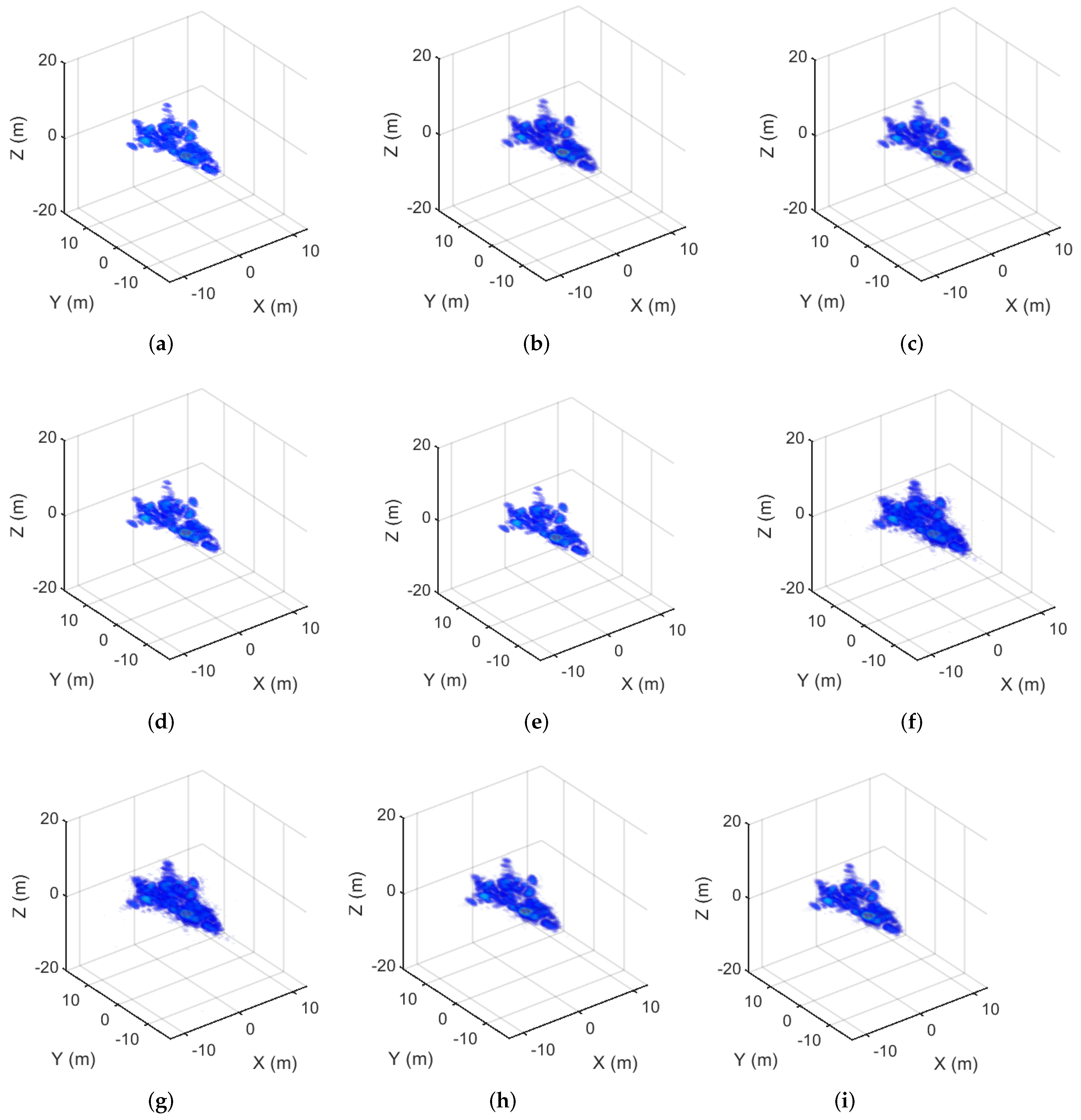
In this section, taking the Section 4.2 aircraft model as an example, we illuminate the calculation time and phase-retention ability of the algorithms in this paper. The dimension of the 3D image matrix are $512\times 101\times 101$. We compare the calculation times of the proposed algorithms in this paper with the iterative soft threshold algorithm (IST) for $L_1$ regularization based on the observation matrix [11]. The calculation times of the different algorithms at sampling rates of 100% are listed in

Table 9. The Time, TBR and ENT of the Aircraft.

Method	Time (s)	TBR (dB)	ENT
IST	48,019.97	56.8645	0.0995
MM-$L_1$ with PI	1.73	55.1236	0.1037
MM-$L_1$ without PI		55.0183	0.1056
MM-$L_{1/2}$ with PI	6.16	56.4521	0.0853
MM-$L_{1/2}$ without PI		56.2314	0.0855
MM-$L_0$ with PI	2.75	53.5286	0.1069
MM-$L_0$ without PI		53.4768	0.1088
GMM-$L_{0.8}$ with PI	6.63	55.1743	0.0988
GMM-$L_{0.8}$ without PI		55.1651	0.0991

. The calculation time of the IST is 48,019.97 s. The calculation times of MM-$L_1$, MM-$L_{1/2}$, MM-$L_0$, and GMM-$L_{0.8}$ are 1.73 s, 6.16 s, 2.75 s, and 6.63 s, respectively. Even considering the calculation time of MF (542.71 s), the calculation time of the proposed algorithms in this paper was significantly lower compared with those of IST.

To compare the imaging performance of the proposed algorithms with IST, we present the imaging results of full sampling data in Figure 11. The TBR and ENT values are listed in Table 9. MM-$L_1$, MM-$L_{1/2}$, MM-$L_0$, and GMM-$L_{0.8}$ achieve equivalent imaging results to those of IST from the fully sampled raw data.

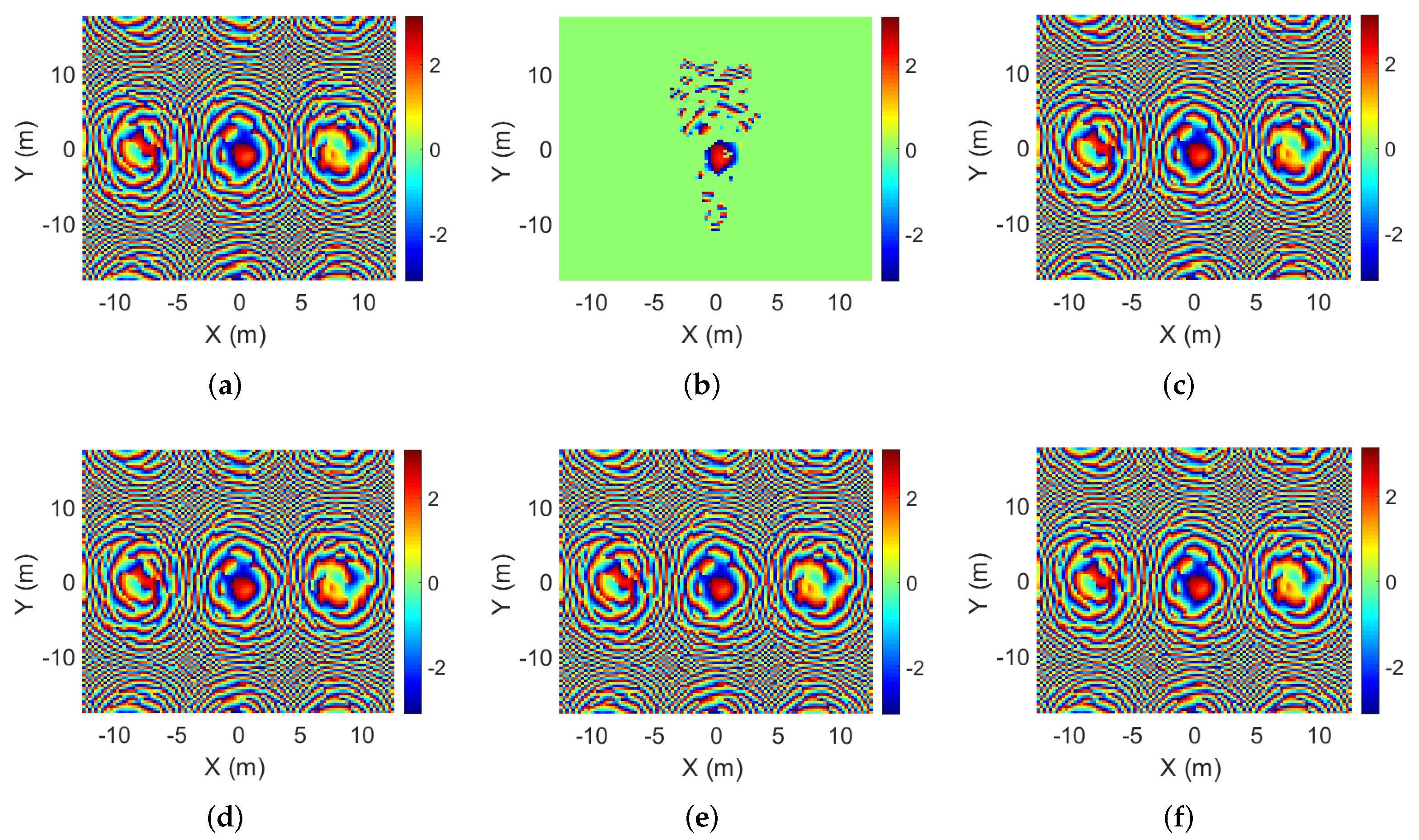
In addition, the proposed algorithms can also obtain imaging results that retain scene-phase information. Figure 12a shows the reference phase. Figure 12b–f show the phase slices of IST, MM-$L_1$, MM-$L_{1/2}$, MM-$L_0$, and GMM-$L_{0.8}$, respectively. Figure 13a–e show the difference between the reference phase and the phase slices of the reconstructed images. The values of each point in the phase difference between the proposed algorithms and the reference phase are 0. The algorithms in this paper can obtain 3D images with phase information, while the IST algorithm, based on the observation matrix, cannot retain phase information.

Finally, taking GMM as an example, we verify the reconstruction performance of the proposed algorithm under lower sampling rates (50%, 25%, and 10%). Figure 14 shows the GMM-$L_{0.8}$ imaging results at sampling rates of 50%, 25%, and 10%. The results show that the quality of the reconstructed image will decrease, and the noise and sidelobe suppression effect will decrease if the sampling rate continues to decrease. With a continuous decrease of the sampling rate, the proposed method will not be able to reconstruct the target scene successfully when the downsampling ratio is less than 25%.

6. Conclusions

In this study, a novel 3D sparse SAR reconstruction method combining the MM framework and $L_q$ regularization was proposed. Firstly, MM-$L_1$, MM-$L_{1/2}$, and MM-$L_0$ were presented to solve the $L_1$, $L_{1/2}$, and $L_0$ regularization optimization problem, respectively. Although the above three methods can improve SAR image quality, they are all intended for use on some specific values of q. Therefore, a generalized $L_q$$\left(0\le q\le 1\right)$ method GMM-$L_q$ was proposed to obtain high-quality 3D SAR images. Compared with MF methods, the proposed methods can effectively improve image quality, such as sidelobe and noise suppression. Compared with the existing observation-matrix-based sparse reconstruction method, the methods in this article significantly reduce computation time. In addition, the proposed method both improves the image quality and preserves the phase information of the complex image. Therefore, the reconstructed complex image can be used in the field when phase information is required. The 3D simulation is used to verify the effect of the proposed method. Finally, real ground-based array SAR data is also used to demonstrate the effectiveness and universality of the method in a real environment. In future research, we will study novel sparse imaging methods based on convolutional neural networks to achieve 3D SAR image with higher accuracy and efficiency.

References

- Cumming, I.G.; Wong, F.H. Digital Signal Processing of Synthetic Aperture Radar Data: Algorithms and Implementation. Artech House 2004, 1, 108–110. [Google Scholar]
- Moses, R.L.; Potter, L.C.; Çetin, M. Wide angle SAR Imaging. In Proceedings of the International Society for Optics and Photonics in Defense and Security, Orlando, FL, USA, 2 September 2004; pp. 164–175. [Google Scholar]
- Wang, Z.M.; Guo, Q.J.; Tian, X.Z. 3-D millimeter-wave imaging using MIMO RMA with range compensation. IEEE Trans. Microwave Theory Tech. 2019, 67, 1157–1166. [Google Scholar] [CrossRef]
- Gui, S.; Li, J.; Pi, Y. Security imaging for multi-target screening based on adaptive scene segmentation with terahertz radar. IEEE Sens. J. 2019, 19, 2675–2684. [Google Scholar] [CrossRef]
- Wang, Y.; Zhang, X.; Zhan, X.; Zhang, T.; Zhou, L.; Shi, J.; Wei, S. An RCS Measurement Method Using Sparse Imaging Based 3D SAR Complex Image. IEEE Antennas Wirel. Propag. Lett. 2021. [Google Scholar] [CrossRef]
- Gao, J.K.; Qin, Y.L.; Deng, B. A novel method for 3-D millimeter-wave holographic reconstruction based on frequency interferometry techniques. IEEE Trans. Microwave Theory Tech. 2017, 66, 1579–1596. [Google Scholar] [CrossRef]
- Salvetti, F.; Martorella, M.; Giusti, E. Multi-view three-dimensional interferometric inverse synthetic aperture radar. IEEE Trans. Aerosp. Electron. Syst. 2018, 55, 718–733. [Google Scholar] [CrossRef]
- Xin, W.; Lu, Z.; Weihua, G.; Pcng, F. Active Millimeter-Wave Near-Field Cylindrical Scanning Three-Dimensional Imaging System. In Proceedings of the 2018 International Conference on Microwave and Millimeter Wave Technology (ICMMT), Chengdu, China, 7–11 May 2018; pp. 1–3. [Google Scholar]
- Bamler, R. A comparison of range-Doppler and wavenumber domain SAR focusing algorithms. IEEE Trans. Geosci. Remote Sens. 1992, 30, 706–713. [Google Scholar] [CrossRef]
- Xiang, J.; Dong, Y.; Yang, Y. FISTA-Net: Learning A Fast Iterative Shrinkage Thresholding Network for Inverse Problems in Imaging. IEEE Trans. Med. Imaging 2021, 99, 1329–1339. [Google Scholar] [CrossRef]
- Daubechies, I.; Defriese, M.; De Mol, C. An iterative thresholding algorithm for linear inverse problems with a sparsity constraint. Commun. Pure Appl. Math. 2004, 57, 1413–1457. [Google Scholar] [CrossRef] [Green Version]
- Beck, A.; Teboulle, M. A Fast Iterative Shrinkage-Thresholding Algorithm for Linear Inverse Problems. SIAM J. Imaging Sci. 2009, 2, 183–202. [Google Scholar] [CrossRef] [Green Version]
- Xu, Z.; Zhang, B.; Zhou, G.; Zhong, L.; Wu, Y. Sparse SAR Imaging and Quantitative Evaluation Based on Nonconvex and TV Regularization. Remote Sens. 2021, 13, 1643. [Google Scholar] [CrossRef]
- Ao, D.; Wang, R.; Hu, C.; Li, Y. A Sparse SAR Imaging Method Based on Multiple Measurement Vectors Model. Remote Sens. 2017, 9, 297. [Google Scholar] [CrossRef] [Green Version]
- Zhang, Q.; Zhang, Y.; Zhang, Y.; Huang, Y.; Yang, J. A Sparse Denoising-Based Super-Resolution Method for Scanning Radar Imaging. Remote Sens. 2021, 13, 2768. [Google Scholar] [CrossRef]
- Çetin, M.; Karl, W.C. Feature–enhanced synthetic aperture radar image formation based on nonquadratic regularization. IEEE Trans. Image Process. 2001, 10, 623–631. [Google Scholar] [CrossRef] [Green Version]
- Bhattacharya, S.; Blumensath, T.; Mulgrew, B.; Davies, M. Fast encoding of synthetic aperture radar raw data using compressed sensing. In Proceedings of the 2007 IEEE/SP 14th Workshop on Statistical Signal Processing, Madison, WI, USA, 26–29 August 2007. [Google Scholar]
- Rilling, G.; Davies, M.; Mulgrew, B. Compressed sensing based compression of SAR raw data. In Proceedings of the SPARS’09-Signal Processing with Adaptive Sparse Structured Representations, Saint-Malo, France, 6–9 April 2009; pp. 1–6. [Google Scholar]
- Zhu, X.; Bamler, R. Super–resolution power and robustness of compressive sensing for spectral estimation with application to spaceborne tomographic SAR. IEEE Trans. Geosci. Remote Sens. 2012, 50, 247–258. [Google Scholar] [CrossRef]
- Hu, C.; Wang, L.; Zhu, D.; Loffeld, O. Inverse Synthetic Aperture Radar Sparse Imaging Exploiting the Group Dictionary Learning. Remote Sens. 2021, 13, 2812. [Google Scholar] [CrossRef]
- Tan, X.; Roberts, W.; Li, J.; Stoica, P. Sparse Learning via Iterative Minimization with Application to MIMO Radar Imaging. IEEE Trans. Signal Process. 2011, 59, 1088–1101. [Google Scholar] [CrossRef]
- Austin, C.D.; Ertin, E.; Moses, R.L. Sparse Signal Methods for 3–D Radar Imaging. IEEE J. Sel. Top. Signal Process. 2011, 5, 408–423. [Google Scholar] [CrossRef]
- Zhu, X.; Bamler, R. Tomographic SAR Inversion by L1-Norm Regularization-the Compressive Sensing Approach. IEEE Trans. Geosci. Remote Sens. 2010, 48, 3839–3846. [Google Scholar] [CrossRef] [Green Version]
- Zuo, W.; Meng, D.; Zhang, L.; Feng, X.; Zhang, D. Title of Presentation. A Generalized Iterated Shrinkage Algorithm for Non-convex Sparse Coding. In Proceedings of the 2013 IEEE International Conference on Computer Vision, Sydney, Australia, 1–8 December 2013; pp. 217–224. [Google Scholar]
- Glentis, G.O.; Zhao, K.; Jakobsson, A.; Li, J. Non–Parametric High–Resolution SAR Imaging. IEEE Trans. Signal Process. 2013, 61, 1614–1624. [Google Scholar] [CrossRef]
- Yang, Z.; Zheng, Y.R. A comparative study of compressed sensing approaches for 3-D synthetic aperture radar image reconstruction. Digit. Signal Process. 2014, 32, 24–33. [Google Scholar] [CrossRef]
- Sun, Y.; Babu, P.; Palomar, D.P. Majorization-Minimization Algorithms in Signal Processing, Communications, and Machine Learning. IEEE Trans. Signal Process. 2017, 65, 794–816. [Google Scholar] [CrossRef]
- Fang, J.; Xu, Z.; Zhang, B.; Hong, W.; Wu, Y. Fast Compressed Sensing SAR Imaging Based on Approximated Observation. IEEE J. Sel. Topics Appl. Earth Observ. Remote Sens. 2014, 7, 352–363. [Google Scholar] [CrossRef] [Green Version]
- Bi, H.; Zhang, B.; Zhu, X. Azimuth-range decouple-based L1 regularization method for wide ScanSAR imaging via extended chirp scaling. J. Appl. Remote Sens. 2017, 11, 015007. [Google Scholar] [CrossRef]
- Bi, H.; Bi, G.; Zhang, B.; Hong, W. Complex-Image-Based Sparse SAR Imaging and Its Equivalence. IEEE Trans. Geosci. Remote Sens. 2018, 56, 5006–5014. [Google Scholar] [CrossRef]
- Xu, Z. L1/2 Regularization: A Thresholding Representation Theory and a Fast Solver. IEEE Trans. Neural Netw. Learn. Syst. 2012, 23, 1013–1027. [Google Scholar] [PubMed]
- Tian, B.; Zhang, X.; Li, L.; Pu, L.; Pu, L.; Shi, J.; Wei, S. Fast Bayesian Compressed Sensing Algorithm via Relevance Vector Machine for LASAR 3D Imaging. Remote Sens. 2021, 13, 1751. [Google Scholar] [CrossRef]
- Werness, S.A.S.; Carrara, W.G.; Joyce, L.S.; Franczak, D.B. Moving target imaging algorithm for SAR data. IEEE Trans. Aerosp. Electron. Syst. 1990, 26, 57–67. [Google Scholar] [CrossRef]
- Wei, S.; Zhou, Z.; Wang, M.; Wei, J.; Liu, S.; Shi, J.; Zhang, X.; Fan, F. 3DRIED: A High-Resolution 3-D Millimeter-Wave Radar Dataset Dedicated to Imaging and Evaluation. Remote Sens. 2021, 13, 3366. [Google Scholar] [CrossRef]
Figure 1.
The geometric relationship of target observation.
Figure 2.
The imaging results of the combat vehicle corresponding to the 100% sampling rate. (a) The MF result. (b) The MM- result. (c) The MM- result. (d) The MM- result. (e) The GMM- result.
Figure 3.
The imaging results of the combat vehicle corresponding to the 75% sampling rate. (a) The MF result. (b) The MM- result. (c) The MM- result. (d) The MM- result. (e) The GMM- result.
Figure 4.
The imaging results of the aircraft corresponding to the 100% sampling rate. (a) The MF result. (b) The MM- result. (c) The MM- result. (d) The MM- result. (e) The GMM- result.
Figure 5.
The imaging results of the aircraft corresponding to the 75% sampling rate. (a) The MF result. (b) The MM- result. (c) The MM- result. (d) The MM- result. (e) The GMM- result.
Figure 6.
The experimental scenario. (a) The two spheres. (b) The snip.
Figure 7.
The imaging results of the real ground-based array SAR data corresponding to the 100% sampling rate. (a) The MF result. (b) The MM- result. (c) The MM- result. (d) The MM- result. (e) The GMM- result.
Figure 8.
The imaging results of the real ground-based array SAR data corresponding to the 75% sampling rate. (a) The MF result. (b) The MM- result. (c) The MM- result. (d) The MM- result. (e) The GMM- result.
Figure 9.
The imaging results of real complex target SAR data corresponding to the 100% sampling rate. (a) The MF result. (b) The MM- result. (c) The MM- result. (d) The MM- result. (e) The GMM- result.
Figure 10.
The imaging results of real complex target SAR data corresponding to the 75% sampling rate. (a) The MF result. (b) The MM- result. (c) The MM- result. (d) The MM- result. (e) The GMM- result.
Figure 11.
The imaging results of the aircraft corresponding to fully sampled data. (a) The The IST result. (b) The MM- result with PI. (c) The MM- result without PI. (d) The MM- result with PI. (e) The MM- result without PI. (f) The MM- result with PI. (g) The MM- result without PI. (h) The GMM- result with PI. (i) The GMM- result without PI.
Figure 12.
Phase slices. (a) The reference phase. (b) The IST result. (c) The MM- result. (d) The MM- result. (e) The MM- result. (f) The GMM- result.
Figure 13.
Phase differences. (a) The difference between IST and the reference phase. (b) The difference between MM- and the reference phase. (c) The difference between MM- and the reference phase. (d) The difference between MM- and the reference phase. (e) The difference between GMM- and the reference phase.
Figure 14.
The imaging results of the GMM-. (a) The MF result corresponding to the 50% sampling rate. (b) The MF result corresponding to the 25% sampling rate. (c) The MF result corresponding to the 10% sampling rate. (d) The GMM- result corresponding to the 50% sampling rate. (e) The GMM- result corresponding to the 25% sampling rate. (f) The GMM- result corresponding to the 10% sampling rate.