
ShadowDeNet: A Moving Target Shadow Detection Network for Video SAR

School of Information and Communication Engineering, University of Electronic Science and Technology of China, Chengdu 611731, China
*
Author to whom correspondence should be addressed.
Remote Sens. 2022, 14(2), 320; https://0-doi-org.brum.beds.ac.uk/10.3390/rs14020320
Submission received: 2 December 2021
/
Revised: 24 December 2021
/
Accepted: 24 December 2021
/
Published: 11 January 2022
(This article belongs to the Special Issue Artificial Intelligence-Based Learning Approaches for Remote Sensing)
Abstract
:Most existing SAR moving target shadow detectors not only tend to generate missed detections because of their limited feature extraction capacity among complex scenes, but also tend to bring about numerous perishing false alarms due to their poor foreground–background discrimination capacity. Therefore, to solve these problems, this paper proposes a novel deep learning network called “ShadowDeNet” for better shadow detection of moving ground targets on video synthetic aperture radar (SAR) images. It utilizes five major tools to guarantee its superior detection performance, i.e., (1) histogram equalization shadow enhancement (HESE) for enhancing shadow saliency to facilitate feature extraction, (2) transformer self-attention mechanism (TSAM) for focusing on regions of interests to suppress clutter interferences, (3) shape deformation adaptive learning (SDAL) for learning moving target deformed shadows to conquer motion speed variations, (4) semantic-guided anchor-adaptive learning (SGAAL) for generating optimized anchors to match shadow location and shape, and (5) online hard-example mining (OHEM) for selecting typical difficult negative samples to improve background discrimination capacity. We conduct extensive ablation studies to confirm the effectiveness of the above each contribution. We perform experiments on the public Sandia National Laboratories (SNL) video SAR data. Experimental results reveal the state-of-the-art performance of ShadowDeNet, with a 66.01% best f1 accuracy, in contrast to the other five competitive methods. Specifically, ShadowDeNet is superior to the experimental baseline Faster R-CNN by a 9.00% f1 accuracy, and superior to the existing first-best model by a 4.96% f1 accuracy. Furthermore, ShadowDeNet merely sacrifices a slight detection speed in an acceptable range.
1. Introduction
Synthetic aperture radar (SAR) is an advanced Earth observation remote sensing tool. Its active radar-based remote sensing ensures its all-day and all-weather working advantage compared with optical sensors [1,2,3]. Thus, so far, it has been widely applied in civil fields, such as marine exploration, forestry census, topographic mapping, land resources survey, and traffic control, as well as military fields, such as battlefield reconnaissance, war situation monitoring, radar guidance, and strike effect evaluation [4,5,6]. Video SAR provides continuous multi-SAR images of the target imaging area to dynamically monitor the target scene in real time. It can continuously record the changes of the target area and exhibit the information from the time dimension through the form of visual active images, conducive to the intuitive interpretation of human eyes [7]. Thus, it is receiving extensive attention from increasing scholars [8,9,10].
Moving target tracking is one of the most significant applications using video SAR. It can provide the important information such as the geographical location, moving direction [11], moving route, and speed of high-value targets in real time [12]. Obviously, it contributes to ground traffic management and accurate attack of military targets. Thus, it has become a research hotspot in recent years [7,13]. So far, some scholars [11,12,13,14,15,16,17,18,19,20,21,22,23,24,25,26,27,28,29,30] have proposed various methods for video SAR moving target tracking that offered competitive results.
Notably, it is interesting that the commonality of the above video SAR moving target tracking methods is to indicate the real moving target with the help of the target’s shadow. This is because in video SAR, the Doppler modulation of the moving target echo is rather sensitive to target motion due to the extremely high working frequency, so a slight motion will lead to the large target location offset and target defocus in SAR images, as shown in Figure 1. However, the above phenomena do not happen on the shadow of the moving target [7], thus the shadow reflects the real position and motion state information of the moving target. More formation mechanisms of the moving target shadows in video SAR can be found in [17].
Especially, moving target shadows are very informative from the following two aspects [7]. On the one hand, the contrast between the moving target shadow and its background area, and the gradient information of the shadow intensity along the moving direction, are both closely related to the target speed. On the other hand, because the synthetic aperture time of a single frame image is short, the dynamic shadow also reflects the instantaneous position of the moving target in the scene [7]. Thus, using shadows to complete the video SAR moving target detection and tracking task has become a new research pathway. Furthermore, combined with the Doppler processing technology, the shadow detection can also greatly expand the detectable velocity range of moving targets and improve the robustness of trackers further.
To summarize, moving target shadow detection in video SAR is extremely important and valuable. It is a fundamental and significant prerequisite of the moving target tracking. Only after the shadow is detected successfully can a subsequent series of tasks be carried out smoothly, such as trajectory filtering/reconstruction [14], data association (i.e., target ID allocation), transformation discrimination between old target disappearance and new one appearance (i.e., target ID switching), velocity estimation [31], SAR image refocusing [11,12], and so on. More descriptions about the relationship between detection and tracking can be found in [32,33]. Thus, this paper will research this valuable work emphatically, that is, video SAR moving target shadow detection. So far, various methods or algorithms [16,17] have been proposed for video SAR moving target shadow detection. These methods can be summarized as two types—(1) traditional feature extraction methods and (2) modern deep learning methods.
The traditional feature extraction methods are based on hand-designed features using expert experience. Wang et al. [10] used a constant false alarm rate (CFAR) detector to detect the moving target shadow, but CFAR is very sensitive to ground clutters, resulting in poor migration ability. Zhong et al. [14] designed a cell-average CFAR based on the mean filtering for the shadow detection, but their method relied heavily on the manual model parameter adjustment. Worse still, their detector was provided with weak capacity to suppress false alarms, which brought huge burdens to the follow-up tracker. Zhao et al. [15] proposed a visual saliency-based detection mechanism based on the image contrast to enhance target shadow to improve discrimination performance by using an adaptive threshold. However, the shadow of the moving target is very dim [16], and easy to submerge by surrounding clutters, leading to its less-salient features. Tian et al. [16] proposed a region-partitioning-based algorithm to search for shadows, but this algorithm suffered from too-complex mathematical theories, with poor flexibility, extensibility, and adaptability. Liu et al. [17] proposed a local feature analysis method based on the OTSU’s method [18] to detect moving target shadows, but their method needed to model background clutters which is challenging for various backgrounds. Zhang et al. [19] proposed a Tsallis-entropy-based [34] segmentation threshold algorithm to classify background pixels and shadow pixels but obtaining the optimal threshold in the complex mathematical equations is rather time-consuming. Shang et al. [20] leveraged the idea of change detection to detect moving target shadows in THz video-SAR images based on their own private terahertz radar system, but change detection (i.e., background subtraction) worked only on strictly static backgrounds and was sensitive to clutters. He et al. [21] proposed an improved difference-based moving target shadow detection method where the morphological filtering was used to suppressed false alarms. However, their approach required a series of well-designed and complicated preprocessing techniques, reducing the application scope of the method. They improved their previous method [21] in the report of [22] using the speeded-up robust features (SURF) algorithm [35], but computational costs were greatly increased. In short, the above traditional methods are all heavy in computation, weak in generalization, and troublesome in manual feature extraction. Moreover, they are both time-consuming and labor-consuming.
Modern deep learning methods mainly draw support from multilayer neural networks to automatically extract features based on given training samples. In the computer vision (CV) community, many deep learning-based methods using convolutional neural networks (CNNs) have boosted object detection performance greatly, e.g., Faster R-CNN [36], feature pyramid network (FPN) [37], you only look once (YOLO) [38], RetinaNet [39], and CenterNet [40]. Some scholars [41,42] have applied them to detection and classification. Nowadays, many scholars in the video SAR community also have applied them for moving target shadow detection. Ding et al. [24] applied Faster R-CNN to detect shadows, but the raw Faster R-CNN is designed for generic objection detection in optical natural images, so their direct use without critical thinking might be controversial if not considering the targeted video SAR task. Wen et al. [25] adopted dual Faster R-CNN detectors to simultaneously detect shadows in the image spatial domain and range-Doppler (RD) spectrum domain. However, the shadow features in image spatial domain were not comprehensively mined by them, which led to missed detections and false alarms once the raw video SAR echo was not available. Huang et al. [26] proposed an improved Faster R-CNN to boost the per-frame features by incorporating the spatiotemporal information extracted from multiple adjacent frames using 3D CNNs, which improved shadow detection performance. However, for the online shadow detection, it is impossible to draw support from the future image sequences to establish a spatiotemporal information space so as to enhance the past image sequences. Moreover, this method must require an accurate registration, a fixed scene, and a constant number of sequence images [17]. These strict requirements are bound to limit algorithm applications in the velocity-independent continuous tracking radar mode of video SAR, which often has a constantly changing scene [17]. Therefore, to achieve more flexible moving detection and tracking, one should better detect shadows using single-frame images [17]. Yan et al. [27] adopted FPN to detect shadows using their self-developed video MiniSAR system. They used the k-means to cluster video SAR targets, and then regarded the results as the basis for setting anchor box scales, so as to speed up network convergence and improve accuracy. However, their preset anchor box cannot resist shadow deformation once the motion speed is changed. Therefore, their model is powerless for noncooperative enemy moving targets. Zhang et al. [28] also used FPN to detect shadows and added a dense local regression module to boost shadow location performance. However, their experimental dataset only contains some simple scenes, which is not enough to confirm the universality of the proposed method. Hu et al. [29] adopted YOLOv3 equipped with FPN to provide initial shadow detection results for the follow-up tracker on the basis of the joint detector embedding model (JDE) [33]. However, YOLOv3 may be not robust enough for more complex scenes. Additionally, in SAR surveillance videos, moving target shadows usually occupy relatively few pixels resulting in their small shape appearance, which is rather challenging to capture with YOLOv3 due to its poor small detection performance [40,41]. Wang et al. [30] adopted CenterNet [40] to detect shadows inspired by FairMOT [43] and CenterTrack [44], but this kind of anchor-free detector still lacks the capacity to deal with complex scenes and cases [45], bringing about many missed detections and false alarms. It should be noted that Lu et al. [46] proposed a RetinaTrack for online single-stage joint detection and tracking where RetinaNet [39] was used to detect targets. Future scholars can also use RetinaNet to detect moving target shadows, because it solves the problem of extreme imbalance between foregrounds and backgrounds by introducing a focal loss. This imbalance is universal for SAR images. Thus, we will apply this focal loss for moving target shadow detection, for the first time, in this paper. To sum up, although the above existing deep learning-based moving target shadow detectors have achieved competitive detection results, their provided detection performance is still limited. For one thing, they tend to generate missed detections due to their limited feature-extraction capacity among complex scenes. For another thing, they also tend to bring about numerous perishing false alarms due to their poor foreground–background discrimination capacity.
Therefore, to handle the above problems, this paper proposes a novel deep learning network named ShadowDeNet for better moving target shadow detection in video SAR images. There are five core contributions to ensure the excellent performance of Shadow-DeNet. These are (1) a histogram equalization shadow enhancement (HESE) preprocessing technique is used for enhancing shadow saliency (i.e., contrast ratio) to facilitate the follow-up feature extraction, (2) a transformer self-attention mechanism (TSAM) is proposed for paying more attention to regions of interests to suppress clutter interferences, (3) a shape deformation adaptive learning (SDAL) network is designed based on deformable convolutions [47] for learning moving target deformed shadows to conquer motion speed variations, (4) a semantic-guided anchor-adaptive learning (SGAAL) network is designed for achieving optimized anchors to adaptively match shadow location and shape, and (5) an online hard-example mining (OHEM) training strategy [48] is adopted for selecting typical difficult negative samples to boost background discrimination capacity. We conduct extensive ablation studies to confirm the effectiveness of the above each contribution. Finally, the experimental results on the open Sandia National Laboratories (SNL) video SAR data [49] reveal the state-of-the-art moving target shadow performance of ShadowDeNet, compared with the other five competitive methods. Specifically, ShadowDeNet is better than the experimental baseline Faster R-CNN by a 9.00% f1 accuracy, and it is also superior to the existing first-best model by a 4.96% f1 accuracy. Furthermore, ShadowDeNet merely sacrifices a slight detection speed in an acceptable range.
2. Methodology
ShadowDeNet is based on the mainstream two-stage framework Faster R-CNN [36]. A two-stage detector usually has better detection accuracy than a one-stage one [40], so we select the former as our experimental baseline in the paper. Figure 2 shows the shadow detection framework of ShadowDeNet. Faster R-CNN consists of a backbone network, a region proposal network (RPN), and a Fast R-CNN [36]. HESE is a preprocessing tool. TSAM and SDAL are used to improve the feature extraction ability of the backbone network. SGAAL is used to improve the proposal generation ability of RPN. OHEM is used to improve the detection ability of Fast R-CNN.
From Figure 2, we first preprocess the input video SAR images using the proposed HESE technique to enhance shadow’s saliency or contrast ratio. The detailed descriptions are introduced in Section 2.1. Then, a backbone network is used to extract shadow features. In ShadowDeNet, without losing generality, we select the commonly-used ResNet-50 [50] as the backbone network. One can leverage more advanced backbone network which may achieve better performance, but this is beyond the scope of this article. In the backbone network, the proposed TSAM and SDAL are embedded, which can both enable better feature extraction. The former is used to pay more attention to regions of interests to suppress clutter interferences based on the attention mechanism [51], which is introduced in detail in Section 2.2. The latter is used to adapt to moving target deformed shadows to overcome motion speed variations based on deformable convolutions [47], which is introduced in detail in Section 2.3.
Immediately, the feature maps are inputted into an RPN to generate regions of interests (ROIs) or proposals. In RPN, a classification network outputs a 2k-dimension vector to represent a proposal category, i.e., a positive or negative sample. Here, k denotes the number of anchor boxes, which is set to nine in line with the raw Faster R-CNN. The determination of positive and negative samples is based on the intersection over union (IOU), also called Jaccard distance [52,53], with the corresponding ground truth (GT). Similar to the original Faster R-CNN, IOU > 0.70 means positive samples, while IOU < 0.30 means negative samples. Samples with 0.30 < IOU < 0.70 are discarded. Moreover, a regression network outputs a 4k-dimension vector to represent a proposal location and shape, i.e., (x, y, w, h), where (x, y) denotes the proposal central coordinate, w denotes the width, and h denotes the height. Regression is performed to locate shadows in essence, whose inputs are the feature maps extracted by the backbone network, and outputs are the possible locations of shadows. In RPN, the proposed SGAAL is inserted to improve the quality of proposals. It can generate optimized anchors to adaptively match shadow location and shape inspired by the works of [23,45], which are introduced in detail in Section 2.4.
Afterwards, one ROIAlign layer [54] is used to map the proposals to the feature maps in the backbone network for the subsequent refined classification and regression. Note that the raw Faster R-CNN used one ROIPooling layer to reach such aim, but we replace it with ROIAlign because ROIAlign can address the problem of misalignments caused by twice-quantization [54] so as to avoid a feature loss. Finally, the refined classification and regression are completed by Fast R-CNN [55] to output the final shadow detection results. Moreover, in training, in Fast R-CNN, OHEM is applied to select typical difficult negative samples to boost background discrimination capacity inspired by the works of [48,53], which are introduced in detail in Section 2.5.
Next, we introduce HESE, TSAM, SDAL, SGAAL, and OHEM in detail in the following subsections.
2.1. Histogram Equalization Shadow Enhancement (HESE)
Moving target shadows in video SAR images are rather dim [16] and are always easy to be submerged by surrounding clutters, leading to their less-salient features from the human vision perspective. Figure 3 shows a video SAR image and the corresponding shadow ground truths. In Figure 3a, it is difficult for human vision to find the shadow of a moving target quickly and clearly if one does not refer to the ground truths in Figure 3b. The contrast between the shadow and the surrounding is very low, resulting in their unclear appearances. Moreover, the patrol gate made of metal materials also poses serious negative effects to shadow detection. This experimental data is introduced in detail in Section 3.1. Therefore, to perform some image preprocessing means is necessary, otherwise the learning benefits of features would be reduced.
Many previous scholars proposed various techniques for image preprocessing, e.g., denoising [8], pixel density clustering [24], morphological filtering [17], visual saliency-based enhancement [15], etc. However, they all rely heavily on expert experience with a series of cumbersome steps, reducing model flexibility. Therefore, we come up with the simple but effective histogram equalization to preprocess video SAR images. For brevity, we denote this process as the histogram equalization shadow enhancement (HESE).
For a video SAR image I, if ni denotes the number of occurrences of the gray value i 0 ≤ i < 256, then the occurrence probability of pixels with the gray value i is
where n denotes the number of all pixels in the image, and pI(i) denotes, actually, the histogram of the image with pixel value i, normalized to [0, 1]. The HESE is described by
Figure 4 shows the image histogram of the image in Figure 3a before HESE and after HESE. From Figure 4, after HESE, the whole gray value distribution (marked in red) is similar to the uniform distribution, so this image has a large gray dynamic range and high contrast, and the details of the image are richer. In essence, HESE is used to stretch the image nonlinearly, and redistribute the image pixel values so that the number of pixel values in a certain gray range is roughly equal. In this way, the contrast of the peak part in the middle of the original histogram is enhanced, while the contrast of the valley bottom part on both sides is reduced. Finally, the contrast of the entire image increases.
Figure 5 shows the moving target shadow enhancement results. From Figure 5, one can clearly find that after HESE, the shadow in the zoom region becomes clearer. In Figure 5a, the raw shadow is hardly captured by human eye vision, but in Figure 5b, anyone can find the shadow quickly and easily. We also evaluate the shadow quality in the zoom region by using the classic 4-neighborhood method [56]. The evaluation results are shown in Table 1. From Table 1, the shadow contrast with HESE is far larger than that without HESE (29,215.43 >> 20,979.31). The shadow contrast enhancement reaches up to ~40%, i.e., (29,215.43–20,979.31)/20,979.31. Moreover, the running time is just 13.06 ms, i.e., 7.66 images per second. This seems to be acceptable. Compared to many previous preprocessing means [8,15,17,24], HESE is rather fast with a rather simple theory and workflow. Readers can find more shadow enhancement results of other frames (#3, #13, #23, #33) in Figure 6.
2.2. Transformer Self-Attention Mechanism (TSAM)
Attention mechanisms are widely used in the CV community that can adaptively learn feature weights to focus on important information and suppress the useless. So far, scholars from the SAR community have applied it to various applications, e.g., SAR automatic target recognition (ATR) [57,58], SAR target detection [59,60] and classification [61,62], and so on. Recently, transformer detectors [63,64] have received increasing concerns in the CV community. The remarkable characteristic of transformer models is the internal self-attention mechanism which is able to effectively capture some important long-range dependencies among the entire location space [65]. In video SAR images, there are many clutter interferences from Figure 3a, so we adopt such self-attention mechanism to suppress them so as to focus on more valuable regions of interests. We call this process transformer self-attention mechanism (TSAM). Specifically, we insert TSAM to the backbone network which enables efficient information flow to extract more representative features. As mentioned before, we selected ResNet-50 as our backbone network in Figure 2, thus we insert TSAM to the residual block to promote better residual learning, as is shown in Figure 7.
In Figure 7, the first 1 × 1 convolution (conv) is used to reduce the input channel dimension, and the second 1 × 1 conv is used to increase the output channel dimension for the follow-up adding operation. The 3 × 3 conv is used to extract shadow features. TSAM is used behind the 3 × 3 conv, meaning that the extracted shadow features are prescreened by TSAM. In this way, the important features are retained while the useless interferences are suppressed. The above practice is similar to that in the convolutional block attention module (CBAM) [66] and squeeze-and-excitation (SE) [67], which can be described as
where F denotes the input of a residual block, F’ denotes the output, f1×1(∙) denotes the 1 × 1 conv operation, f3×3(∙) denotes the 3 × 3 conv operation, and TSAM(∙) denotes the operation.
Figure 8 shows the detailed implementation process of TSAM. In Figure 8, H denotes the height of the input feature map X, H denotes the width, and C denotes the channel number. According to Wang et al. [68], the general transformer self-attention can be summarized as
where i is the index of the required output location (i.e., the response of the i-th location is to be calculated), and j is the index that enumerates all possible locations, i.e., ∀j. x denotes the input feature map, and y denotes the output feature map with the same dimension as x. The paired function f computes the relationship between i and all j. The unary function g calculates the representation of the input feature map at the j-th location. Finally, the response is normalized by a factor C(x).
The paired function f can be achieved by an embedded Gaussian function so as to compute similarity between i and all j in an embedding space, i.e.,
where θ denotes the embedding of xi and ϕ denotes the embedding of xj. From Figure 8, they are implemented by using two 1 × 1 convs Wθ and Wϕ. That is, θ(xi) = Wθxi and ϕ(xj) = Wϕxj. Here, to reduce the computation cost, their kernel numbers are set to C/2 if the input channel number is C. The normalization factor is set as C(x) = Σ∀jf(xi, xj). Thus, for a given i, f(xi, xj)/C(x) will become the softmax computation along the dimension j where softmax is defined by [69]. Here, the softmax computation is responsible for generating the weight (i.e., importance level) of each location. Similarly, the representation of the input feature map at the j-th location is also calculated in an embedding space by using another one 1 × 1 conv Wg. With the matrix multiplication, the output of the self-attention Y is obtained. Finally, in order to complete the residual operation (i.e., adding), one 1 × 1 conv Wz is used to increase the channel number from C/2 to C, i.e.,
In essence, TSAM is able to calculate the interaction between any two positions and also directly captures the remote dependence without being limited to adjacent points. It is equivalent to constructing a convolution kernel as large as the size of the feature map, so that more background context information can be maintained. In this way, the network can focus on important regions of interests to suppress clutter interferences or other negative effects of useless backgrounds.
2.3. Shape Deformation Adaptive Learning (SDAL)
The contrast between the shadow generated by the moving target and its background area, the gradient information of the shadow intensity along the moving direction, and the shape of the shadow are all closely related to the moving speed of the target [7]. On the premise that the shadow can be formed, the smaller the moving speed of the target, the greater the shadow extension [70], and the clearer the shadow contour of the moving target. However, the larger the moving speed of the target, the lower the shadow extension, and the more blurred the shadow contour of the moving target. In other words, when the motion speed of the moving target changes, the shadow shape will change. When the motion speed changes continuously in multiframe video SAR images, the shadow of the same target will become deformed. This challenges the robustness of the detector. Readers can refer to [11] for more details about the shadow size relationship with the speed.
Figure 9 shows the moving target shadow deformation with the change of moving speed. In Figure 9, due to the stopping signal of the traffic light, the vehicle-A’s speed is becoming smaller and smaller. One can find that the same vehicle-A exhibits shadows with different shapes (the zoom region) in the different frames in the video SAR. Thus, a good shadow detector should resist such shadow deformation. However, the feature extraction process of classical convolution neural networks mainly depends on convolution kernels, but the geometric structure of traditional convolution kernel is fixed. Only fixed local feature information is extracted each time when a convolution operation is performed. Thus, the classical convolution cannot solve the shape deformation problem. Fortunately, the recent deformation convolution proposed by Dai et al. [47] can overcome this problem because its convolution kernel can produce free deformation to adapt to the geometric deformation of the target. The deformable convolution changes the sampling position of the standard convolution kernel by adding additional offsets at the sampling points. The compensation obtained can be learned through training without additional supervision. We call the above shape deformation-adaptive learning (SDAL).
Figure 10 is the sketch map of different convolutions. From Figure 10, the deformation convolution can resist shadow deformation effectively by the learned location offsets. Figure 11 shows the implementation of SDAL.
The standard convolution kernel is augmented with offsets ∆pn which are adaptively learned in training to model various shape features, i.e.,
where p0 denotes each location, ℜ denotes the convolution region, w denotes the weight parameters, x denotes the input, y denotes the output, and ∆pn denotes the learned offsets in the n-th location. ∆pn is typically fractional, so the bilinear interpolation is used to ensure the smooth implementation of convolution, i.e.,
where g(a,b) = max(0, 1–|a–b|). We add another convolution layer (marked in purple in Figure 11) to learn the offsets ∆pn, and then, the standard convolution combining ∆pn is performed on the input feature maps. Moreover, inspired by [47], the traditional convolutions of the high-level layers, i.e., conv3_x, conv4_x, conv5_x in ResNet-50, are replaced with deformation ones to extract more robust shadow features. This is because the slightest change in the receptive field size among the high-level layers is able to pose a remarkable difference to the following networks, thus obtaining a better geometric modeling capacity in transformation of shape-changeable moving target shadows [71].
2.4. Semantic-Guided Anchor-Adaptive Learning (SGAAL)
Anchors are the basis in modern object detection, which are usually a set of artificially designed boxes, used as the benchmark for classification and bounding box regression. However, previous video SAR moving target shadow detectors mostly adopt preset fixed-shape or fixed-size or fixed-scale anchors. In other words, they have changeless scales and aspect ratios, potentially declining the feature learning benefits of moving target shadows. Moreover, the raw anchors are arranged in the feature map densely and uniformly and are not in line with the video SAR image characteristic, as in Figure 12a. This is because moving target shadows in video SAR images are distributed sparsely and unevenly; if the dense and uniform anchors are used, there will be many false alarms generated. Therefore, inspired by Wang et al. [45], we design a novel semantic-guided anchor-adaptive learning (SGAAL) tool to generate high-quality location-adaptive and shape-adaptive anchors in the RPN, as in Figure 12b. Here, we adopt the high-level deep semantic features to guide anchor generation which can ensure higher anchor quality [45].
The aim of SGAAL is to adaptively obtain the anchor location and the corresponding shape, that is, the parameters (x, y, w, h) of anchors in the image I, where (x, y) denotes the spatial coordinate of the anchor center, w denotes the width of the anchor box, and h denotes the height of the anchor box. Therefore, SGAAL can be described by
where p(x, y|I) denotes the prediction process of the anchor location for a given image I, and p(w, h|x, y, I) denotes the prediction process of the anchor shape for a given image I and the corresponding known location. In other words, SGAAL will first adaptively predict the location (x, y) of anchors, and then adaptively predict the shape (w, h) of anchors. Figure 13 shows the detailed implementation process of SGAAL. In Figure 13, the input semantic feature is denoted by Q. Its height is denoted by H, its width is denoted by W, and its channel number is denoted by C.
From Figure 13, we use a 1 × 1 conv WL to predict the anchor location whose channel number is set to 1, which will encode the whole H × W location space. This 1 × 1 conv layer is followed by a sigmod activation function that is defined by 1/(1 + e−x) to represent the occurrence probability of the shadow location. Here, the location threshold is denoted by εL. That is, when the value of the location (x, y) is bigger than εL, then this location is assigned by a positive “1” label (i.e., the network should generate anchors at this location); otherwise, it is assigned by a negative “0” label (i.e., the network should not generate anchors at this location). As locations with shadows occupy a small portion of the whole feature map, we adopt the focal loss (FL) of RetinaNet [39] to train this anchor location prediction network so as to avoid falling into a large number of negative samples, i.e.,
where y denotes the ground-truth class. y = 1 means the positive, otherwise it is the negative. p denotes the predicted probability ranging from 0 to 1. γ denotes the focusing parameter, set to 2 empirically, and αt denotes the weighting factor, set to 0.25 empirically.
We use a 1 × 1 conv WS to predict the anchor shape whose channel number is set to 2 because we need to obtain the anchor width w and height h. The anchor shape prediction is across the whole H × W location space. However, the shape predictions whose corresponding location predictions are lower than the threshold εL are filtered. This threshold εL will be determined experimentally in Section 5.4. The bounded IOU loss [72] is used to train this anchor shape prediction network because it is more sensitive to box spatial locations, i.e.,
where G denotes the ground-truth box and P denotes the prediction box.
As a result, the anchor location and shape are obtained combined with WL and WS. Note that Wang et al. [45] pointed out that the feature for a large anchor should encode the content over a large region, while those for small anchors should have smaller scopes accordingly, thus, following their practice, we also devise an anchor-guided feature adaptation component, which will transform the feature at each individual location i based on the underlying anchor shape, i.e.,
where qi denotes the i-th location element of the raw feature map Q, and qi’ denotes the i-th location element of the transformed feature map Q’, and wi and hi denote the width and height of anchors at the i-th location. Moreover, A is a 3 × 3 deformable convolutional layer WA which is used to predict the offset field from the output of the anchor shape prediction branch, and then apply the learned offset to the original feature map to obtain the final feature map Q’.
Finally, based on the adaptively learned anchors, the high-quality proposals are generated, and then they are mapped to the transformed feature map Q’ by ROIAlign to extract their corresponding feature regions for the subsequent classification and regression in Fast R-CNN, as in Figure 2. In this way, the obtained optimized anchors will be able to adaptively match shadow location and shape so as to enable better false-alarm suppression ability and ensure more attentive shadow feature learning.
2.5. Online Hard-Example Mining (OHEM)
SGAAL can remove many negative samples by the location judgment, but it still does not solve the imbalance problem between positive samples and negative samples. For a location in the feature map, the number of the generated negative samples is still far more than that of positive ones, because background pixels usually occupy a larger proportion. Among a large number of negative samples, it is necessary to select more typical difficult negative samples and abandon easy ones to enhance background discrimination capacity. Online hard-example mining (OHEM) is an advanced difficult-identified negative sample mining method during training. It was proposed by Shrivastava et al. [48] in 2016 and mainly selects some difficult negative samples as training samples in the training process of the target detection model, so as to improve the model parameters and make it converge to a better effect. Difficult samples refer to the samples which are difficult to distinguish, with a large training loss value. For a simple sample that is easy to correctly classify, it is difficult for the model to learning more effective information from it. Thus, hard samples are more valuable for model optimization and are more worth mining and utilization.
Figure 14 shows the detailed implementation process of OHEM. In Figure 14, the classification loss of Fast R-CNN is denoted losscls, and the regression loss is denoted lossreg. We sum the losscls and lossreg of the negative samples. Their sum loss losssum is then ranked, and the top k samples are selected into the hard-negative sample pool, where k is set to 256, inspired by [48]. Moreover, the positive sample number is set to 256 to avoid falling into the local optimization of a certain positive or negative category. When the sample number in the pool reaches a batch size, they are mapped into the feature map by ROIAlign again to be trained repeatedly and emphatically. In this way, Fast R-CNN is able to learn more representative background features to further suppress false alarms. More details can be found in [48].
3. Experiments
Our experiments are all performed on a personal computer (PC) which is equipped with an NVIDIA GeForce RTX 3090 GPU, an Intel(R) Core(TM) i9-10900KF CPU, and 32 G memory based on the Pytorch [73] and MMDetection [74] software development environment using the Python language. Furthermore, CUDA-11.1 and CuDNN-8.0.5 are both used for the training and inference GPU acceleration.
3.1. Data
We conduct experiments on the public data released by Sandia National Laboratories [49]. This video SAR data is the only publicly available, thus it is selected. It is the video SAR footage of a gate at the Kirtland Air Force Base Eubank Gate. Table 2 shows the radar system parameters of this data. Figure 15 shows the experimental working environment of the optical image and the corresponding SAR image.
There are 900 frames of continuous SAR images in the SNL video data. The image size is 660 pixel × 720 pixel. We divide the raw video into nine sub-videos, i.e., one sub-video contains 100 continuous SAR image sequences. The moving target shadow ground truths are labeled by professional experts. The first six sub-videos, i.e., 600 continuous SAR images, are selected as the training dataset. The remaining three sub-videos, i.e., 300 continuous SAR images, are selected as the test dataset. This data is available https://www.sandia.gov/app/uploads/sites/124/2021/08/eubankgateandtrafficvideosar.mp4 (accessed on 20 November 2021) where related scholars can download it for free for scientific research.
3.2. Experimental Details
We train ShadowDeNet based on the stochastic gradient descent (SGD) optimizer [75] by 12 epochs. The learning rate is set to 0.008, the momentum is set to 0.9, and the weight decay is set to 0.0001. The training warmup is the linear mode with 500 iterations. The learning rate is reduced by 10 times at the 8th and the 11th epoch. The training batch size is set to four because of the limited GPU memory. The input image size of ShadowDeNet is 660 pixel × 720 pixel. To avoid overfitting, the ImageNet pretrained weights [76] of ResNet-50 [50] are loaded for transfer learning. Other network parameters are initialized using the Kaiming method [77]. Other hyperparameters not mentioned are same as Faster R-CNN. During inference, the nonmaximum suppression (NMS) [78] is used to suppress duplicate detection boxes with an IOU threshold of 0.50.
3.3. Evaluation Indices
The PASCAL VOC evaluation indices [79] are adopted whose detection IOU threshold is 0.50.
The recall (r) is defined by
where tp denotes the true positives (i.e., correct detections), fn denotes the false negatives (i.e., missed detections), and # denotes the number. In essence, r is equal to the detection rate Pd.
The precision (p) is defined by
where fp denotes the false positives (i.e., false alarms). In essence, p is equal to 1 − Pf (the false alarm rate).
The average precision (ap) is defined by
where p(r) denotes the precision-recall curve.
The f1-score is defined by
In this paper, we mainly use f1 as the core accuracy index because it can make a trade-off between the detection rate and the false alarm rate regardless of if in the traditional machine learning community or in the modern deep learning community.
We use the frames per second (FPS) to measure the detection speed, defined by
where T denotes the time consumed to complete an image detection.
4. Results
4.1. Quantitative Results
Table 3 shows the quantitative results of ShadowDeNet on the SNL video SAR data. In Table 3, we show the quantitative results by the mean of progressively adding the proposed improvements to the experimental baseline Faster R-CNN [36]. More ablation studies about the impact of each improvement on the whole ShadowDeNet model are introduced in Section 5 by the mean of each installation and removal.
From Table 3, one can draw the following conclusions:
- The detection accuracy presents a rising trend by progressively adding the proposed improvements to the experimental baseline Faster R-CNN. This confirms the effectiveness of each technique. In terms of the f1 accuracy, it has increased from the initial 57.01% to 66.01%, up to a 9.00% huge improvement. In terms of the ap accuracy, it has increased from the initial 46.33% to 51.87%, up to a 5.54% observable improvement. Other accuracy indexes are also increased, more or less. This fully reveals the extraordinary moving target shadow detection performance.
- HESE improves the ap accuracy by ~3.5% and the f1 accuracy by ~2.5%, showing its effectiveness. It can improve the detection rate (r is increased from 55.91% to 56.80%), meanwhile suppressing false alarms (p is increased from 58.16% to 62.45%), because it can enhance shadow saliency for robust shadow feature extraction and strong background discrimination. As presented before in Section 2.1, the enhanced shadow becomes more prominent and clearer and becomes easier and more intuitive to capture for human eye vision. This resulting benefit is also helpful for the network feature adaptive learning.
- TSAM improves the ap accuracy marginally, but the f1 accuracy is still improved by ~0.7%. It is still useful for shadow detection because it can detect more real shadows, i.e., the number of correct detections is increased from 898 to 903 (that is, the previous five missed detections are detected successfully again by using TSAM), meanwhile it still can suppress many false alarms, i.e., the number of false alarms is reduced from 540 to 516 (that is, the previous 24 false alarms are suppressed thoroughly by using TSAM). From the comparison results, TSAM seems to be able to enable better false alarm suppress ability, which is in fact in line with its internal working mechanism introduced in Section 2.2. That is, it can receive more contextual information to focus more on regions of interests and suppress clutter interferences. As a result, the exhibited results indicate the lower false alarm rate when TSAM is used.
- SDAL improves the ap accuracy by ~1.1% and the f1 accuracy by ~3.0%. The latter’s improvement is larger than the former’s. This is because the latter is more sensitive to the false alarm rate, which is exactly in line with the fact that SDAL is able to suppress false alarms greatly, i.e., the p is increased from 63.64% to 69.85%. SDAL can also detect another five real shadows, because it can find the shadows with intense deformations again when the motion speed is changed, as introduced in Section 2.3. Moreover, we hold the view that when SDAL is used, the network generalization ability can be enhanced, because the network can adapt to “moving” target shadow deformations so as to reduce the possibility of falling into the local optimization among a large number of the “static” dark shadow-like background negative samples. Consequently, the false alarm rate is decreased greatly.
- SGAAL offers an almost similar ap accuracy, but it still improves the f1 accuracy by ~1.75%. This f1 accuracy improvement is from the increase of p, that is, from 69.85% to 74.59%. This phenomenon exactly accords with the theoretical analysis in Section 2.4. SGAAL can filter many dense anchors using its anchor location prediction network. As a result, the anchors become sparser in line with the sparse distribution of moving shadows in the video SAR images. Moreover, it should be noted that SGAAL seems not to improve the detection rate from the above results but declines it a little, but this does not mean that its anchor shape prediction network is useless, because another experiment in Section 5.4 shows that it still plays an important role in the whole fully-equipped ShadowDeNet (that is, when the other four improvements are used, only SGAAL is removed).
- OHEM further decreases the false alarm rate, i.e., the p is improved from 74.59% to 78.30%. As a result, the ap accuracy is improved from the previous 50.33% to the final 51.87%, and the f1 accuracy is improved from the previous 64.73% to the final 66.01%. This is because OHEM can mine difficult negative samples and train them repeatedly and emphatically, as introduced in Section 2.5. Finally, the foreground–background discrimination capacity of the model can be boosted.
- Each improvement offers different accuracy gains. The accuracy growth rate is also different when one of them is inserted. The overall change trend of accuracy is constantly upward. However, the internal synergistic effects between different improvements are difficult to figure out thoroughly. This will need extensive experiments to study further. It is impossible for this paper to exhaustively complete all combination of experiments in the current state. They can be arranged in the future. Despite all this, the scientific value of this paper is not completely affected.
Table 4 shows the performance comparison with the other five state-of-the-art detectors. From Table 4, this paper mainly selects the Faster R-CNN, FPN, YOLOv3, RetinaNet, and CenterNet to conduct performance comparison. They are all trained using the video SAR data of this paper again. Their implementations are basically the same as their original reports. Their backbone networks also load the ImageNet pretrained weights so as to ensure the comparison fairness. Moreover, we indeed know that there might be more other advanced generic deep learning object detection models in the CV community; however, they have not been applied for video SAR moving shadow detection so far by scholars in the SAR community. Therefore, we do not compare ShadowDeNet with them because this paper is limited in the SAR community. On the contrary, Faster R-CNN, FPN, YOLOv3, RetinaNet, and CenterNet have been applied for video SAR moving shadow detection by Ding et al. [24], Wen et al. [25], Huang et al. [26], Yan et al. [27], Zhang et al. [28], Hu et al. [29], Wang et al. [30], and so on, so they are selected. Moreover, various signs of the existing state indicate that deep learning methods have far exceeded most traditional methods, so we leave out the comparison with traditional methods that are usually based on excessive manual features.
From Table 4, one can draw the following conclusions:
- ShadowDeNet achieves the best accuracy for the video SAR moving shadow detection regardless of the ap index or the f1 index. Although the ap index of ShadowDeNet is slightly better than FPN, its f1 index is far superior to FPN, i.e., 66.01% >> 61.05%, about a ~5% accuracy improvement. Notably, FPN generates much more false alarms than ShadowDeNet, i.e., 504 >> 250. As a result, the p index of FPN is far lower than that of ShadowDeNet, i.e., 64.51% << 78.30%, about such a huge 14% gap. Therefore, the above reveals the state-of-the-art moving target shadow performance of ShadowDeNet.
- ShadowDeNet offers a huge accuracy gain based on the experimental baseline Faster R-CNN. The total accuracy gain is up to ~1.14% in terms of the r index, ~20.14% in terms of the p index, ~5.54% in terms of the ap index, and ~9.00% in terms of the f1 index. These all benefit from the five improvement methods used as introduced before.
- ShadowDeNet merely sacrifices a slight detection speed compared with the experimental baseline Faster R-CNN, i.e., from 15.79 FPS to 11.11 FPS. Therefore, ShadowDeNet is cost-effective. It can sacrifice a relatively weak speed in exchange for a huge increase in accuracy, demonstrating its advanced nature.
- CenterNet offers the fastest detection speed, i.e., 27.27 FPS, but its detection accuracy is too poor to satisfy actual application requirements, i.e., its 33.69% f1 << ShadowDeNet’s 66.01% f1. Moreover, the poor detection performance of CenterNet might be from its anchor-free mechanism based on the keypoint detection, because in video SAR images, the energy of the moving target shadow is rather weak, resulting in the shadow’s rather few keypoints.
- The two-stage detectors (Faster R-CNN and FPN) achieve the better accuracy performance than the one-stage ones (YOLOv3, RetinaNet, and CenterNet). However, the detection speed of the two-stage detectors is universally slower than that of the one-stage ones. This phenomenon is in line with the common sense in the CV community, because RPNs in two-stage detectors usually consume more time while enabling better box detection accuracy.
Figure 16 shows the accuracy changing curves (r, p, ap, and f1) of different methods when the IOU threshold is set increasingly. From Figure 16, when the IOU threshold becomes bigger and bigger, the accuracy becomes poorer and poorer. This is in line with common sense, because a larger IOU threshold will challenge the box regression performance seriously. Furthermore, except the recall–IOU curve in Figure 16a, most accuracy–IOU curves of ShadowDeNet are on the upper of all other curves, especially for the f1–IOU curve in Figure 16d, which shows the better detection performance of ShadowDeNet. The results in Table 4 are at an IOU threshold of 0.50, the same as the PASCAL VOC criterion [79]. Finally, from Figure 16, one can find that it is rather necessary to further improve the box location performance. In the future, scholars should better design stronger coordinate positioning networks to ensure better performance at a large IOU threshold.
4.2. Qualitative Results
Figure 18 shows the qualitative moving target shadow detection results of different methods. In Figure 18, the display confidence threshold of Faster R-CNN, FPN, YOLOv3, RetinaNet, and ShadowDeNet is 0.50. However, CenterNet does not offer the similar classification confidence scores. In Figure 18f, the numbers above boxes denote CenterNet’s Gaussian heatmap probabilities of the top five keypoints. Here, we exhibit the shadow detection results of the 601st, 772nd, 806th, and 900th frames.
From Figure 18, one can draw the following conclusions:
- ShadowDeNet can avoid many missed detections (marked by red ellipses). If taking the 900th frame as an example, most other methods always miss more shadows than ShadowDeNet, e.g., three missed detections of Faster R-CNN, 3, three ones of FPN, four ones of YOLOv3, and so on, which are all more than that of ShadowDeNet (only two missed detections).
- ShadowDeNet can suppress many false alarms (marked by orange boxes). If taking the 806th frame as an example, most other methods generate more false alarms than ShadowDeNet, e.g., one false alarm of Faster R-CNN, two ones of FPN, three ones of RetinaNet, and so on, which are all more than that of ShadowDeNet (no false alarms).
- ShadowDeNet can offer comparable confidences of shadows. For example, the vehicle marked by a green triangle has a 0.99 confidence for Faster R-CNN, a 0.98 confidence for FPN, a 0.72 confidence for YOLOv3, a 0.94 confidence for RetinaNet, a 0.41 confidence for CenterNet, and a 0.90 confidence for ShadowDeNet. As CenterNet does not offer classification confidences, we omit the confidence comparisons of different confidence thresholds. Otherwise, it is unfair for CenterNet. For example, if we regard the Gaussian heatmap probabilities of CenterNet as the classification confidences, and set the confidence threshold to 0.50, CenterNet will miss all vehicles. This is obviously unreasonable. Moreover, ShadowDeNet’s confidences are slightly lower than Faster R-CNN and FPN. This disadvantage will be solved in the future.
- ShadowDeNet offers the most advanced video SAR moving target shadow detection performance compared to all the five state-of-the-art methods.
5. Ablation Study
In this section, we carry out some ablation studies of each characteristic in ShadowDeNet. The impact of each characteristic on the whole ShadowDeNet model performance will be introduced by the mean of each installation and removal.
5.1. Ablation Study on HESE
Table 5 shows the quantitative detection results of ShadowDeNet with and without HESE. From Table 5, HESE can improve the overall performance of ShadowDeNet by ~4.0% f1 accuracy, which shows its effectiveness. This is because HESE can enhance the shadow saliency and its contrast ratio, as shown in Figure 5 and Table 1, so as to enable the better follow-up feature extraction of the backbone network. When the shadow is enhanced, the discrimination between foreground and background is bound to become more relaxing. Of course, one may adopt more advanced techniques to further highlight the shadow for better performance, but HESE might be the most direct and easiest tool without complex theory and cumbersome steps.
Moreover, we also select the adaptive histogram equalization shadow enhancement (AHESE) to discuss the shadow detection performance impacts. There are two hyperparameters in AHESE, i.e., the limited contrast ratio, and the size of blocks. We set the limited contrast ratio to 2.0, and set the size of blocks to 8, which are both default values in OpenCV [80]. Figure 19 shows the comparison results of HESE and AHESE. From Figure 19, AHESE does not make backgrounds brighter than HESE. It seems that HESE performs a little bit better than AHESE from human eye visual observation, because the shadows enhanced by HESE are clearer than those enhanced by AHESE. Moreover, from the yellow ellipse regions in Figure 19, the shadows enhanced by AHESE are more easily submerged by the similar black backgrounds. This is one reason why we use HESE.
We make a quantitative assessment of HESE and AHESE in Table 6. From Table 6, AHESE does not offer better f1 accuracy than HESE (64.87% < 66.01%), but it offers better ap accuracy than HESE (53.33% > 51.87%). Therefore, HESE is comparable to AHESE on our experimental data. Considering that AHESE not only consumes more time than HESE but also adds another two hyperparameters requiring trouble-manual adjustments [81], we select the most classic HESE as the preprocessing tool.
5.2. Ablation Study on TSAM
Table 7 shows the quantitative detection results of ShadowDeNet with and without TSAM. From Table 7, TSAM can improve the overall performance of ShadowDeNet by ~3.2% f1 accuracy, which shows its effectiveness. Combined with TSAM, the network can adaptively learn differential spatial information weight to pay more attention to shadow regions rather than background ones, which will enable to detect more shadows and suppress false alarms. As a result, the detection rate is increased by ~1.0% and the false alarm rate is decrease by ~8.0% from Table 7. Furthermore, TSAM can, in fact, calculate the interaction relationship between any two positions and also directly captures the remote dependence without being limited to adjacent points. In this way, more background context information can be maintained. Note that related scholars can adopt other more advanced attention mechanisms [82] to boost detection performance further. Yet, this paper does not study it in depth any more at present. We can continue this task in the future.
5.3. Ablation Study on SDAL
Table 8 shows the quantitative detection results of ShadowDeNet with and without SDAL. From Table 8, SDAL can improve the overall performance of ShadowDeNet by ~3.8% f1 accuracy, which shows its effectiveness. This is because SDAL can model the geometric deformations of the moving target shadow to adapt to motion speed variations. Finally, ShadowDeNet can discriminate the static backgrounds and the moving target shadows more effectively. Of course, SDAL is not free, and it usually needs more time to learn the kernel offsets of Equation (7) in training. However, once the kernel offsets have been learned, the speed sacrifice in the inference or test process is insignificant.
5.4. Ablation Study on SGAAL
Table 9 shows the quantitative detection results of ShadowDeNet with and without SGAAL. From Table 9, SDAL can improve the overall performance of ShadowDeNet by ~2.8% f1 accuracy and ~3% ap accuracy, which shows its effectiveness. For one thing, its internal anchor location network can predict shadow-like regions adaptively to suppress false alarms. For another thing, its internal anchor shape network can predict better shapes to match moving target shadows adaptively to improve the detection rate. As a result, the false alarm rate is dropped by ~2.3%; meanwhile, the detection rate is increased by ~3.0%.
We perform another experiment to study the impact of the location filter threshold εL. The quantitative results are shown in Table 10. In Table 10, the value range of εL is suggested by Wang et al. [45]. From Table 10, when εL is set to 0.01, the accuracy reaches the best. Thus, the final εL is set to 0.01 in ShadowDeNet. Our experimental results are in line with [45] where εL is also set to 0.01. According to their findings, a small location filter threshold has already removed many false positives. However, a too-large location filter threshold is bound to remove many true positives, resulting in a lower detection rate. We find that such phenomenon is also in line with video SAR images.
5.5. Ablation Study on OHEM
Table 11 shows the quantitative detection results of ShadowDeNet with and without OHEM. From Table 11, SDAL can improve the overall performance of ShadowDeNet by ~1.3% f1 accuracy and ~1.5% ap accuracy, which shows its effectiveness. Although the detection rate is not very sensitive to OHEM, the false alarm rate is decreased greatly by ~4.0% when OHEM is used. This is because OHEM can mine hard negative samples and train them repeatedly and emphatically. Finally, the foreground–background discrimination ability of ShadowDeNet can be boosted further.
6. Discussion
We also discuss the shadow detection performance of ShadowDeNet on another video SAR dataset to reveal its universal effectiveness and excellent migration ability. This data is provided by Zhou et al. [12] and China Aerospace Science and Industry Corporation (CASIC) 23 research institute. This data was obtained from the spotlight SAR that was equipped on an aircraft and flew along a circular trajectory at a height of 3000 m. The carrier frequency, resolution, and velocity of aircraft are Ka-band, 0.15 m, and 80 m/s. There are 369 images with 1000 × 1000 pixel size. Among them, 246 images are selected as the training set, and the remaining 123 images are selected as the test set.
Figure 20 shows the qualitative results of ShadowDeNet on the CASIC 23 research institute video SAR data, and the quantitative results are shown in Table 12. From Figure 20, many moving target shadows can be detected by ShadowDeNet successfully, showing the excellent migration ability of ShadowDeNet. From Table 12, ShadowDeNet offers comparable shadow detection performance on the CASIC 23 research institute video SAR data with the SNL video SAR data, i.e., 66.01% f1 vs. 66.28% f1 and 52.39% ap vs. 51.87% ap. Therefore, ShadowDeNet is effective on video SAR data, showing its universal effectiveness.
7. Conclusions
This paper proposes a novel deep learning network ShadowDeNet for the moving target shadow detection from video SAR images. Five characteristics are used to guarantee ShadowDeNet’s superior detection performance, i.e., (1) HESE, which is used to enhance shadow saliency to facilitate feature extraction, (2) TSAM, which is used to focus on regions of interests to suppress clutter interferences, (3) SDAL, which is used to learn moving target deformed shadows adaptively to conquer motion speed variations, (4) SGAAL, which is used to generate optimized anchors to match shadow location and shape, and (5) OHEM, which is used to select typical difficult negative samples to improve background discrimination capacity. Finally, the quantitative and qualitative results reveal the state-of-the-art detection performance of ShadowDeNet with a 66.01% best f1 accuracy. Specifically, it is superior to the experimental baseline Faster R-CNN by a 9.00% f1 accuracy. It is also superior to the existing best model by a 4.96% f1 accuracy. Moreover, the detection speed sacrifice is very slight. Last but not least, we also conduct extensive ablation studies on the public SNL video SAR data to confirm the effectiveness of each characteristic. We also use ShadowDeNet to detect shadows on another one video SAR data, and the results reveal its universal effectiveness and excellent migration ability. In short, ShadowDeNet can provide high-quality predetection results for subsequent trackers, of great value.
Our future work is as follows:
- We will improve the detection rate of ShadowDeNet further in the future.
- We will conduct the subsequent target association and the trajectory reconstruction tasks.
- We will postprocess the current obtained detection results to remove missed detections and suppress false alarms further by using the multiframe relationship.
- Traditional features can be considered to be injected into CNN-based models to improve performance further.
Author Contributions
Conceptualization, T.Z.; methodology, T.Z.; software, J.B.; validation, X.X.; formal analysis, J.B.; investigation, J.B.; resources, T.Z.; data curation, J.B.; writing—original draft preparation, T.Z. and J.B.; writing—review and editing, T.Z., J.B. and X.Z.; visualization, X.Z.; supervision, X.Z.; project administration, T.Z.; funding acquisition, X.Z. All authors have read and agreed to the published version of the manuscript.
Funding
This work was supported in part by the National Key R&D Program of China under Grant 2017YFB0502700 and in part by the National Natural Science Foundation of China under Grants 61571099, 61501098, and 61671113.
Institutional Review Board Statement
Not applicable.
Informed Consent Statement
Not applicable.
Data Availability Statement
No new data were created or analyzed in this study. Data sharing is not applicable to this article. The public video SAR data provided by Sandia National Laboratories (SNL) is available from https://www.sandia.gov/app/uploads/sites/124/2021/08/eubankgateandtrafficvideosar.mp4 (accessed on 20 November 2021) to download for scientific research. China Aerospace Science and Industry Corporation (CASIC) 23 research institute video SAR data is not public because of copyright restrictions.
Acknowledgments
The authors would like to thank the editors and anonymous reviewers for their valuable comments that greatly improve our manuscript. The authors would like to thank Sandia National Laboratories (SNL) and China Aerospace Science and Industry Corporation (CASIC) 23 research institute for providing the video SAR data.
Conflicts of Interest
The authors declare no conflict of interest.
References
- Moreira, A.; Prats-Iraola, P.; Younis, M.; Krieger, G.; Hajnsek, I.; Papathanassiou, K.P. A Tutorial on Synthetic Aperture Radar. IEEE Geosci. Remote Sens. Mag. 2013, 1, 6–43. [Google Scholar] [CrossRef] [Green Version]
- Zhang, T.; Zhang, X.; Shi, J.; Wei, S. Depthwise Separable Convolution Neural Network for High-Speed SAR Ship Detection. Remote Sens. 2019, 11, 2483. [Google Scholar] [CrossRef] [Green Version]
- Zhang, T.; Zhang, X. High-Speed Ship Detection in SAR Images Based on a Grid Convolutional Neural Network. Remote Sens. 2019, 11, 1206. [Google Scholar] [CrossRef] [Green Version]
- Zhang, T.; Zhang, X. Shipdenet-20: An Only 20 Convolution Layers and <1-Mb Lightweight SAR Ship Detector. IEEE Geosci. Remote Sens. Lett. 2021, 18, 1234–1238. [Google Scholar] [CrossRef]
- Zhang, T.; Zhang, X.; Shi, J.; Wei, S.; Wang, J.; Li, J.; Su, H.; Zhou, Y. Balance Scene Learning Mechanism for Offshore and Inshore Ship Detection in SAR Images. IEEE Geosci. Remote Sens. Lett. 2020, 19, 4004905. [Google Scholar] [CrossRef]
- Zhang, T.; Zhang, X. Squeeze-and-Excitation Laplacian Pyramid Network with Dual-Polarization Feature Fusion for Ship Classification in SAR Images. IEEE Geosci. Remote Sens. Lett. 2021, 19, 4019905. [Google Scholar] [CrossRef]
- Ding, J. Focusing Algorithms and Moving Target Detection Based on Video SAR. J. Radars 2020, 9, 321–334. [Google Scholar]
- Huang, X.; Xu, Z.; Ding, J. Video SAR Image Despeckling by Unsupervised Learning. IEEE Trans. Geosci. Remote Sens. 2020, 59, 1–10. [Google Scholar] [CrossRef]
- Huang, X.; Ding, J.; Guo, Q. Unsupervised Image Registration for Video SAR. IEEE J. Sel. Top. Appl. Earth Obs. Remote Sens. 2021, 14, 1075–1083. [Google Scholar] [CrossRef]
- Wang, H.; Chen, Z.; Zheng, S. Preliminary Research of Low-RCS Moving Target Detection Based on Ka-Band Video SAR. IEEE Geosci. Remote Sens. Lett. 2017, 14, 811–815. [Google Scholar] [CrossRef]
- Yang, X.; Shi, J.; Zhou, Y.; Wang, C.; Hu, Y.; Zhang, X.; Wei, S. Ground Moving Target Tracking and Refocusing Using Shadow in Video-SAR. Remote Sens. 2020, 12, 3083. [Google Scholar] [CrossRef]
- Zhou, Y.; Shi, J.; Wang, C.; Hu, Y.; Zhou, Z.; Yang, X.; Wei, S. SAR Ground Moving Target Refocusing by Combining Mre3 Network and Tvβ-Lstm. IEEE Trans. Geosci. Remote Sens. 2020, 60, 1–14. [Google Scholar] [CrossRef]
- Damini, A.; Balaji, B.; Parry, C.; Mantle, V. A videoSAR mode for the X-band wideband experimental airborne radar. In Algorithms for Synthetic Aperture Radar Imagery, 17th ed.; International Society for Optics and Photonics: Bellingham, WA, USA, 2010; p. 76990. [Google Scholar] [CrossRef]
- Zhong, C.; Ding, J.; Zhang, Y. Joint Tracking of Moving Target in Single-Channel Video SAR. IEEE Trans. Geosci. Remote Sens. 2021. [Google Scholar] [CrossRef]
- Zhao, B.; Han, Y.; Wang, H.; Tang, L.; Liu, X.; Wang, T. Robust Shadow Tracking for Video SAR. IEEE Geosci. Remote Sens. Lett. 2020, 18, 821–825. [Google Scholar] [CrossRef]
- Tian, X.; Liu, J.; Mallick, M.; Huang, K. Simultaneous Detection and Tracking of Moving-Target Shadows in ViSAR Imagery. IEEE Trans. Geosci. Remote Sens. 2021, 59, 1182–1199. [Google Scholar] [CrossRef]
- Liu, Z.; An, D.; Huang, X. Moving Target Shadow Detection and Global Background Reconstruction for VideoSAR Based on Single-Frame Imagery. IEEE Access. 2019, 7, 42418–42425. [Google Scholar] [CrossRef]
- Otsu, N. A Threshold Selection Method from Gray-Level Histograms. IEEE Trans. Syst. Man. Cybern. Syst. 1979, 9, 62–66. [Google Scholar] [CrossRef] [Green Version]
- Zhang, Y.; Mao, X.; Yan, H.; Zhu, D.; Hu, X. A Novel Approach to Moving Targets Shadow Detection in VideoSAR Imagery Sequence. In Proceedings of the IEEE International Geoscience and Remote Sensing Symposium (IGARSS), Quebec City, QC, Canada, 13–18 July 2014; pp. 606–609. [Google Scholar]
- Shang, S.; Wu, F.; Liu, Z.; Yang, Y.; Li, D.; Jin, L. Moving Target Shadow Detection and Tracking Based on Thz Video-SAR. In Proceedings of the International Conference on Infrared, Millimeter and Terahertz Waves (IRMMW-THz), Houston, TX, USA, 2–7 October 2011; pp. 1–2. [Google Scholar]
- He, Z.; Chen, X.; Yu, C.; Li, Z.; Yu, A.; Dong, Z. A Robust Moving Target Shadow Detection and Tracking Method for VideoSAR. J. Electron. Inf. Technol. 2021, 7, 1–9. [Google Scholar]
- He, Z.; Chen, X.; Yi, T.; He, F.; Dong, Z.; Zhang, Y. Moving Target Shadow Analysis and Detection for ViSAR Imagery. Remote Sens. 2021, 13, 3012. [Google Scholar] [CrossRef]
- Bao, J.; Zhang, X.; Zhang, T.; Shi, J.; Wei, S. A Novel Guided Anchor Siamese Network for Arbitrary Target-of-Interest Tracking in Video-SAR. Remote Sens. 2021, 13, 4504. [Google Scholar] [CrossRef]
- Ding, J.; Wen, L.; Zhong, C.; Loffeld, O. Video SAR Moving Target Indication Using Deep Neural Network. IEEE Trans. Geosci. Remote Sens. 2020, 58, 7194–7204. [Google Scholar] [CrossRef]
- Wen, L.; Ding, J.; Loffeld, O. Video SAR Moving Target Detection Using Dual Faster R-CNN. IEEE J. Sel. Top. Appl. Earth Obs. Remote Sens. 2021, 14, 2984–2994. [Google Scholar] [CrossRef]
- Huang, X.; Liang, D.; Ding, J. Moving Target Detection in Video SAR Based on Improved Faster R-CNN. In Proceedings of the European Conference on Synthetic Aperture Radar (EUSAR), Online Event, 29 March–1 April 2021; pp. 1–5. [Google Scholar]
- Yan, H.; Huang, J.; Li, R.; Wang, X.; Zhang, J.; Zhu, D. Research on Video SAR Moving Target Detection Algorithm Based on Improved Faster Region-based CNN. J. Electron. Inf. Technol. 2021, 43, 615–622. [Google Scholar]
- Zhang, H.; Liu, Z. Moving Target Shadow Detection Based on Deep Learning in Video SAR. In Proceedings of the IEEE International Geoscience and Remote Sensing Symposium (IGARSS), Quebec City, QC, Canada, 13–18 July 2021; pp. 4155–4158. [Google Scholar]
- Hu, Y. Research on Shadow-Based SAR Multi-Target Tracking Method. Master’s Thesis, University of Electronic Science and Technology of China, Chengdu, China, 2021. [Google Scholar]
- Wang, W.; Hu, Y.; Zou, Z.; Zhou, Y.; Wang, C. Video SAR Ground Moving Target Indication Based on Multi-Target Tracking Neural Network. In Proceedings of the IEEE International Geoscience and Remote Sensing Symposium (IGARSS), Quebec City, QC, Canada, 13–18 July 2014; pp. 4584–4587. [Google Scholar]
- Shang, S.; Wu, F.; Zhou, Y.; Liu, Z. Moving Target Velocity Estimation of Video SAR Based on Shadow Detection. In Proceedings of the Cross Strait Radio Science & Wireless Technology Conference (CSRSWTC), Fuzhou, China, 13–16 December 2020; pp. 1–3. [Google Scholar]
- Yu, F.; Li, W.; Li, Q.; Liu, Y.; Shi, X.; Yan, J. POI: Multiple Object Tracking with High Performance Detection and Appearance Feature. In Proceedings of the European Conference on Computer Vision Workshops, Amsterdam, The Netherlands, 8–10 and 15–16 October 2016; pp. 36–42. [Google Scholar]
- Wang, Z.; Zheng, L.; Liu, Y.; Li, Y.; Wang, S. Towards Real-Time Multi-Object Tracking. In Proceedings of the European Conference on Computer Vision, Glasgow, UK, 23–28 August 2020; pp. 107–122. [Google Scholar]
- Anastasiadis, A. Special Issue: Tsallis Entropy. Entropy 2012, 14, 174–176. [Google Scholar] [CrossRef] [Green Version]
- Bay, H.; Ess, A.; Tuytelaars, T.; Gool, L.V. Speeded-Up Robust Features (SURF). Comput. Vis. Image Underst. 2008, 110, 346–359. [Google Scholar] [CrossRef]
- Ren, S.; He, K.; Girshick, R.; Sun, J. Faster R-CNN: Towards Real-Time Object Detection with Region Proposal Networks. IEEE Trans. Pattern Anal. Mach. Intell. 2017, 39, 1137–1149. [Google Scholar] [CrossRef] [Green Version]
- Lin, T.-Y.; Dollar, P.; Girshick, R.; He, K.; Hariharan, B.; Belongie, S. Feature Pyramid Networks for Object Detection. In Proceedings of the IEEE Conference on Computer Vision and Pattern Recognition (CVPR), Honolulu, HI, USA, 21–26 July 2017; pp. 936–944. [Google Scholar]
- Redmon, J.; Farhadi, A. YOLOv3: An Incremental Improvement. arXiv 2018, arXiv:1804.02767. [Google Scholar]
- Lin, T.-Y.; Goyal, P.; Girshick, R.; He, K.; Dollar, P. Focal Loss for Dense Object Detection. IEEE Trans. Pattern Anal. Mach. Intell. 2020, 42, 318–327. [Google Scholar] [CrossRef] [Green Version]
- Duan, K.; Bai, S.; Xie, L.; Qi, H.; Huang, Q.; Tian, Q. CenterNet: Keypoint Triplets for Object Detection. In Proceedings of the IEEE International Conference on Computer Vision (ICCV), Seoul, Korea, 27–28 October 2019; pp. 6568–6577. [Google Scholar]
- Zhang, T.; Zhang, X.; Liu, C.; Shi, J.; Wei, S.; Ahmad, I.; Zhan, X.; Zhou, Y.; Pan, D.; Li, J.; et al. Balance Learning for Ship Detection from Synthetic Aperture Radar Remote Sensing Imagery. ISPRS J. Photogramm. Remote Sens. 2021, 182, 190–207. [Google Scholar] [CrossRef]
- Zhang, T.; Zhang, X. Injection of Traditional Hand-Crafted Features into Modern CNN-Based Models for SAR Ship Classification: What, Why, Where, and How. Remote Sens. 2021, 13, 2091. [Google Scholar] [CrossRef]
- Zhang, Y.; Wang, C.; Wang, X.; Zeng, W.; Liu, W. FairMOT: On the Fairness of Detection and Re-Identification in Multiple Object Tracking. Int. J. Comput. Vis. 2021, 129, 3069–3087. [Google Scholar] [CrossRef]
- Zhou, X.; Koltun, V.; Krähenbühl, P. Tracking Objects as Points. In Proceedings of the European Conference on Computer Vision (ECCV), Graz, Austria, 7–13 May 2006; pp. 474–490. [Google Scholar]
- Wang, J.; Chen, K.; Yang, S.; Loy, C.C.; Lin, D. Region Proposal by Guided Anchoring. In Proceedings of the IEEE Conference on Computer Vision and Pattern Recognition (CVPR), Long Beach, CA, USA, 15–20 June 2019; pp. 2960–2969. [Google Scholar]
- Lu, Z.; Rathod, V.; Votel, R.; Huang, J. RetinaTrack: Online Single Stage Joint Detection and Tracking. In Proceedings of the IEEE Conference on Computer Vision and Pattern Recognition (CVPR), Seattle, WA, USA, 14–19 June 2020; pp. 14656–14666. [Google Scholar]
- Dai, J.; Qi, H.; Xiong, Y.; Li, Y.; Zhang, G. Deformable Convolutional Networks. In Proceedings of the IEEE International Conference on Computer Vision (ICCV), Venice, Italy, 22–29 October 2017; pp. 764–773. [Google Scholar]
- Shrivastava, A.; Gupta, A.; Girshick, R. Training Region-Based Object Detectors with Online Hard Example Mining. In Proceedings of the IEEE Conference on Computer Vision and Pattern Recognition (CVPR), Las Vegas, NV, USA, 27–30 June 2016; pp. 761–769. [Google Scholar]
- National Technology and Engineering Solutions of Sandia. Pathfinder Radar ISR & SAR Systems. Eubank Gate and Traffic VideoSAR. 2021. Available online: http://www.sandia.gov/radar/video (accessed on 30 November 2021).
- He, K.; Zhang, X.; Ren, S.; Sun, J. Deep Residual Learning for Image Recognition. In Proceedings of the IEEE Conference on Computer Vision and Pattern Recognition (CVPR), Las Vegas, NV, USA, 27–30 June 2016; pp. 770–778. [Google Scholar]
- Zhu, X.; Cheng, D.; Zhang, Z.; Lin, S.; Dai, J. An Empirical Study of Spatial Attention Mechanisms in Deep Networks. In Proceedings of the IEEE International Conference on Computer Vision (ICCV), Seoul, Korea, 27–28 October 2019; pp. 6687–6696. [Google Scholar]
- Kosub, S. A Note on the Triangle Inequality for the Jaccard Distance. Pattern Recognit Lett. 2019, 120, 36–38. [Google Scholar] [CrossRef] [Green Version]
- Li, J.; Qu, C.; Shao, J. Ship Detection in SAR Images Based on an Improved Faster R-CNN. In Proceedings of the SAR in Big Data Era: Models, Methods and Applications (BIGSARDATA), Beijing, China, 13–14 November 2017; pp. 1–6. [Google Scholar]
- He, K.; Gkioxari, G.; Dollar, P.; Girshick, R. Mask R-CNN. In Proceedings of the IEEE International Conference on Computer Vision (ICCV), Venice, Italy, 22–29 October 2017; pp. 2980–2988. [Google Scholar]
- Girshick, R. Fast R-CNN. In Proceedings of the IEEE International Conference on Computer Vision (ICCV), Santiago, Chile, 7–13 December 2015; pp. 1440–1448. [Google Scholar]
- Ibrahim, H.; Kong, N.S.P. Brightness Preserving Dynamic Histogram Equalization for Image Contrast Enhancement. IEEE Trans. Consum. Electron. 2007, 53, 1752–1758. [Google Scholar] [CrossRef]
- Zhang, M.; An, J.; Yu, D.H.; Yang, L.D.; Wu, L.; Lu, X.Q. Convolutional Neural Network with Attention Mechanism for SAR Automatic Target Recognition. IEEE Geosci. Remote Sens. Lett. 2020, 19, 4004205. [Google Scholar] [CrossRef]
- Li, R.; Wang, X.; Wang, J.; Song, Y.; Lei, L. SAR Target Recognition Based on Efficient Fully Convolutional Attention Block CNN. IEEE Geosci. Remote Sens. Lett. 2020, 1–5. [Google Scholar] [CrossRef]
- Zhang, T.; Zhang, X.; Shi, J.; Wei, S. Hyperli-Net: A Hyper-Light Deep Learning Network for High-Accurate and High-Speed Ship Detection from Synthetic Aperture Radar Imagery. ISPRS J. Photogramm. Remote Sens. 2020, 167, 123–153. [Google Scholar] [CrossRef]
- Gao, F.; He, Y.; Wang, J.; Hussain, A.; Zhou, H. Anchor-Free Convolutional Network with Dense Attention Feature Aggregation for Ship Detection in SAR Images. Remote Sens. 2020, 12, 2619. [Google Scholar] [CrossRef]
- Zhang, T.; Zhang, X. A Polarization Fusion Network with Geometric Feature Embedding for SAR Ship Classification. Pattern Recognit. 2021, 123, 108365. [Google Scholar] [CrossRef]
- Zhang, T.; Zhang, X.; Ke, X.; Liu, C.; Xu, X.; Zhan, X.; Wei, S. HOG-ShipCLSNet: A Novel Deep Learning Network with Hog Feature Fusion for SAR Ship Classification. IEEE Trans. Geosci. Remote Sens. 2021, 1–22. [Google Scholar] [CrossRef]
- Carion, N.; Massa, F.; Synnaeve, G.; Usunier, N.; Kirillov, A.; Zagoruyko, S. End-to-End Object Detection with Transformers. In Proceedings of the European Conference on Computer Vision (ECCV), Heraklion, Greece, 5–11 September 2010; pp. 213–229. [Google Scholar]
- Zhu, X.; Su, W.; Lu, L.; Li, B.; Wang, X.; Dai, J. Deformable Detr: Deformable Transformers for End-to-End Object Detection. In Proceedings of the International Conference on Learning Representations (ICLR), Addis Ababa, Ethiopia, 26–30 April 2020; p. 12. [Google Scholar]
- Vaidwan, H.; Seth, N.; Parihar, A.S.; Singh, K. A Study on Transformer-Based Object Detection. In Proceedings of the 2021 International Conference on Intelligent Technologies (CONIT), Hubli, India, 25–27 June 2021; pp. 1–6. [Google Scholar]
- Woo, S.; Park, J.; Lee, J.-Y.; Kweon, I.S. Cbam: Convolutional Block Attention Module. In Proceedings of the European Conference on Computer Vision (ECCV), Heraklion, Greece, 5–11 September 2018; pp. 3–19. [Google Scholar]
- Hu, J.; Shen, L.; Albanie, S.; Sun, G.; Wu, E. Squeeze-and-Excitation Networks. IEEE Trans. Pattern Anal. Mach. Intell. 2020, 42, 2011–2023. [Google Scholar] [CrossRef] [Green Version]
- Wang, X.; Girshick, R.; Gupta, A.; He, K. Non-Local Neural Networks. In Proceedings of the IEEE Conference on Computer Vision and Pattern Recognition (CVPR), Salt Lake City, UT, USA, 18–22 June 2018; pp. 7794–7803. [Google Scholar]
- Bishop, M.C. Pattern Recognition and Machine Learning (Information Science and Statistics); Springer: Berlin, Germany, 2006. [Google Scholar]
- Ann Marie, R.; Douglas, L.B.; Armin, W.D. Stationary and Moving Target Shadow Characteristics in Synthetic Aperture Radar. In Proceedings of the Radar Sensor Technology XVIII, Baltimore, MD, USA, 29 May 2014; pp. 1–15. [Google Scholar]
- Ke, X.; Zhang, X.; Zhang, T.; Shi, J.; Wei, S. SAR Ship Detection Based on an Improved Faster R-CNN Using Deformable Convolution. In Proceedings of the IEEE International Geoscience and Remote Sensing Symposium (IGARSS), Seoul, Kore, 25–29 July 2021; pp. 3565–3568. [Google Scholar]
- Tychsen-Smith, L.; Petersson, L. Improving Object Localization with Fitness Nms and Bounded Iou Loss. In Proceedings of the IEEE Conference on Computer Vision and Pattern Recognition (CVPR), Salt Lake City, UT, USA, 18–22 June 2018; pp. 6877–6885. [Google Scholar]
- Ketkar, N. Introduction to Pytorch. Deep Learning with Python: A Hands-On Introduction; Apress: Berkeley, CA, USA, 2017; pp. 195–208. Available online: https://0-link-springer-com.brum.beds.ac.uk/chapter/10.1007/978-1-4842-2766-4_12 (accessed on 1 December 2021).
- Chen, K.; Wang, J.; Pang, J.; Cao, Y.; Xiong, Y.; Li, X.; Lin, D. MMDetection: Open MMLAB Detection Toolbox and Benchmark. arXiv 2019, arXiv:1906.07155. [Google Scholar]
- Goyal, P.; Dollár, P.; Girshick, R.; Noordhuis, P.; Wesolowski, L.; Kyrola, A.; He, K. Accurate, Large Minibatch SGD: Training ImageNet in 1 Hour. arXiv 2017, arXiv:1706.02677. [Google Scholar]
- He, K.; Girshick, R.; Doll´ar, P. Rethinking ImageNet Pre-Training. In Proceedings of the IEEE International Conference on Computer Vision (ICCV), Seoul, Korea, 27–28 October 2019; pp. 4917–4926. [Google Scholar]
- He, K.; Zhang, X.; Ren, S.; Sun, J. Delving Deep into Rectifiers: Surpassing Human-Level Performance on Imagenet Classification. In Proceedings of the IEEE International Conference on Computer Vision (ICCV), Santiago, Chile, 7–13 December 2015; pp. 1026–1034. [Google Scholar]
- Hosang, J.; Benenson, R.; Schiele, B. Learning Non-Maximum Suppression. In Proceedings of the IEEE Conference on Computer Vision and Pattern Recognition (CVPR), Honolulu, HI, USA, 21–26 July 2017; pp. 6469–6477. [Google Scholar]
- Everingham, M.; Eslami, S.M.A.; Gool, L.V.; Williams, C.K.I.; Winn, J.; Zisserman, A. The Pascal Visual Object Classes Challenge: A Retrospective. Int. J. Comput. Vis. 2015, 111, 98–136. [Google Scholar] [CrossRef]
- OpenCV. Available online: https://opencv.org/ (accessed on 30 November 2021).
- Stark, J.A. Adaptive Image Contrast Enhancement Using Generalizations of Histogram Equalization. IEEE Trans. Image Process. 2000, 9, 889–896. [Google Scholar] [CrossRef] [Green Version]
- Niu, Z.; Zhong, G.; Yu, H. A Review on the Attention Mechanism of Deep Learning. Neurocomputing 2021, 452, 48–62. [Google Scholar] [CrossRef]
Figure 1.
Relative positions between the targets and corresponding shadows. This video SAR image is the 731st frame in the SNL data.
Figure 1.
Relative positions between the targets and corresponding shadows. This video SAR image is the 731st frame in the SNL data.

Figure 2.
Shadow detection framework of ShadowDeNet. HESE denotes the histogram equalization shadow enhancement. TSAM denotes the transformer self-attention mechanism. SDAL denotes the shape deformation adaptive learning. SGAAL denotes the semantic-guided anchor-adaptive learning. OHEM denotes the online hard-example mining. In ShadowDeNet, without losing generality, we select the commonly-used ResNet-50 [50] as the backbone network.

Figure 3.
A video SAR image. (a) The raw video SAR image; (b) the shadow corresponding ground truths. Here, different vehicles are marked in boxes with different colors and numbers for an intuitive visual observation. This video SAR image is the 50th frame in the SNL data.
Figure 3.
A video SAR image. (a) The raw video SAR image; (b) the shadow corresponding ground truths. Here, different vehicles are marked in boxes with different colors and numbers for an intuitive visual observation. This video SAR image is the 50th frame in the SNL data.

Figure 4.
Image pixel histogram before HESE and after HESE.

Figure 5.
Moving target shadow before HESE and after HESE. (a) Before HESE; (b) after HESE. The raw video SAR image is in Figure 3a.
Figure 5.
Moving target shadow before HESE and after HESE. (a) Before HESE; (b) after HESE. The raw video SAR image is in Figure 3a.

Figure 6.
More results of the histogram equalization shadow enhancement (HESE). (a) Before HESE; (b) after HESE. Different vehicles are marked in boxes with different colors and numbers for an intuitive visual observation. #N denotes the N-th frame. The white arrows indicate the moving direction.
Figure 6.
More results of the histogram equalization shadow enhancement (HESE). (a) Before HESE; (b) after HESE. Different vehicles are marked in boxes with different colors and numbers for an intuitive visual observation. #N denotes the N-th frame. The white arrows indicate the moving direction.

Figure 7.
Residual block in the backbone network. (a) The raw residual block in ResNet-50; (b) the improved residual block with TSAM.
Figure 7.
Residual block in the backbone network. (a) The raw residual block in ResNet-50; (b) the improved residual block with TSAM.

Figure 8.
Detailed implementation process of TSAM.

Figure 9.
Moving target shadow deformation with the change of moving speed. From left to right (#64 → #74 → #84 → #94), the speed becomes smaller and smaller. The blue arrow indicates the moving direction.
Figure 9.
Moving target shadow deformation with the change of moving speed. From left to right (#64 → #74 → #84 → #94), the speed becomes smaller and smaller. The blue arrow indicates the moving direction.

Figure 10.
Different convolutions. (a) Classical convolution; (b) deformation convolution.

Figure 11.
Detailed implementation process of SDAL.

Figure 12.
Sketch map of different anchor distributions. (a) The raw distribution; (b) the improved distribution with SGAAL. Anchors are marked in blue boxes.
Figure 12.
Sketch map of different anchor distributions. (a) The raw distribution; (b) the improved distribution with SGAAL. Anchors are marked in blue boxes.

Figure 13.
Detailed implementation process of SGAAL.

Figure 14.
Detailed implementation process of OHEM.

Figure 15.
Experimental working environment of the SNL video SAR data at the Kirtland Airforce Base Eubank Gate. (a) The optical image; (b) the corresponding SAR image.
Figure 15.
Experimental working environment of the SNL video SAR data at the Kirtland Airforce Base Eubank Gate. (a) The optical image; (b) the corresponding SAR image.

Figure 16.
The accuracy changing curves with different IOU thresholds of different methods. (a) The curve between recall (r) and IOU; (b) the curve between precision (p) and IOU; (c) the curve between average precision (ap) and IOU; (d) the curve between f1 and IOU.
Figure 16.
The accuracy changing curves with different IOU thresholds of different methods. (a) The curve between recall (r) and IOU; (b) the curve between precision (p) and IOU; (c) the curve between average precision (ap) and IOU; (d) the curve between f1 and IOU.

Figure 17.
Precision–recall (p–r) curves of different methods.

Figure 18.
Qualitative video SAR moving target shadow detection results of different methods. (a) Ground truth; (b) Faster R-CNN; (c) FPN; (d) YOLOv3; (e) RetinaNet; (f) CenterNet; (g) ShadowDeNet. The false alarms are marked by orange boxes. The missed detections are marked by red ellipses. Apart from CenterNet, the numbers above boxes are the confidences. The numbers above boxes in (f) denote CenterNet’s Gaussian heatmap probabilities of the top five keypoints. The IOU threshold is 0.50, the same as the PASCAL VOC criterion [79].


Figure 19.
Different histogram equalization shadow enhancements. (a) Shadows in the raw video SAR image; (b) shadows enhanced by HESE; (c) shadows enhanced by AHESE.
Figure 19.
Different histogram equalization shadow enhancements. (a) Shadows in the raw video SAR image; (b) shadows enhanced by HESE; (c) shadows enhanced by AHESE.

Figure 20.
Qualitative video SAR moving target shadow detection results of ShadowDeNet on the CASIC 23 research institute data. The ground truths are marked by green boxes. The numbers above boxes are the confidences. The IOU threshold is 0.50, the same as the PASCAL VOC criterion [79].
Figure 20.
Qualitative video SAR moving target shadow detection results of ShadowDeNet on the CASIC 23 research institute data. The ground truths are marked by green boxes. The numbers above boxes are the confidences. The IOU threshold is 0.50, the same as the PASCAL VOC criterion [79].


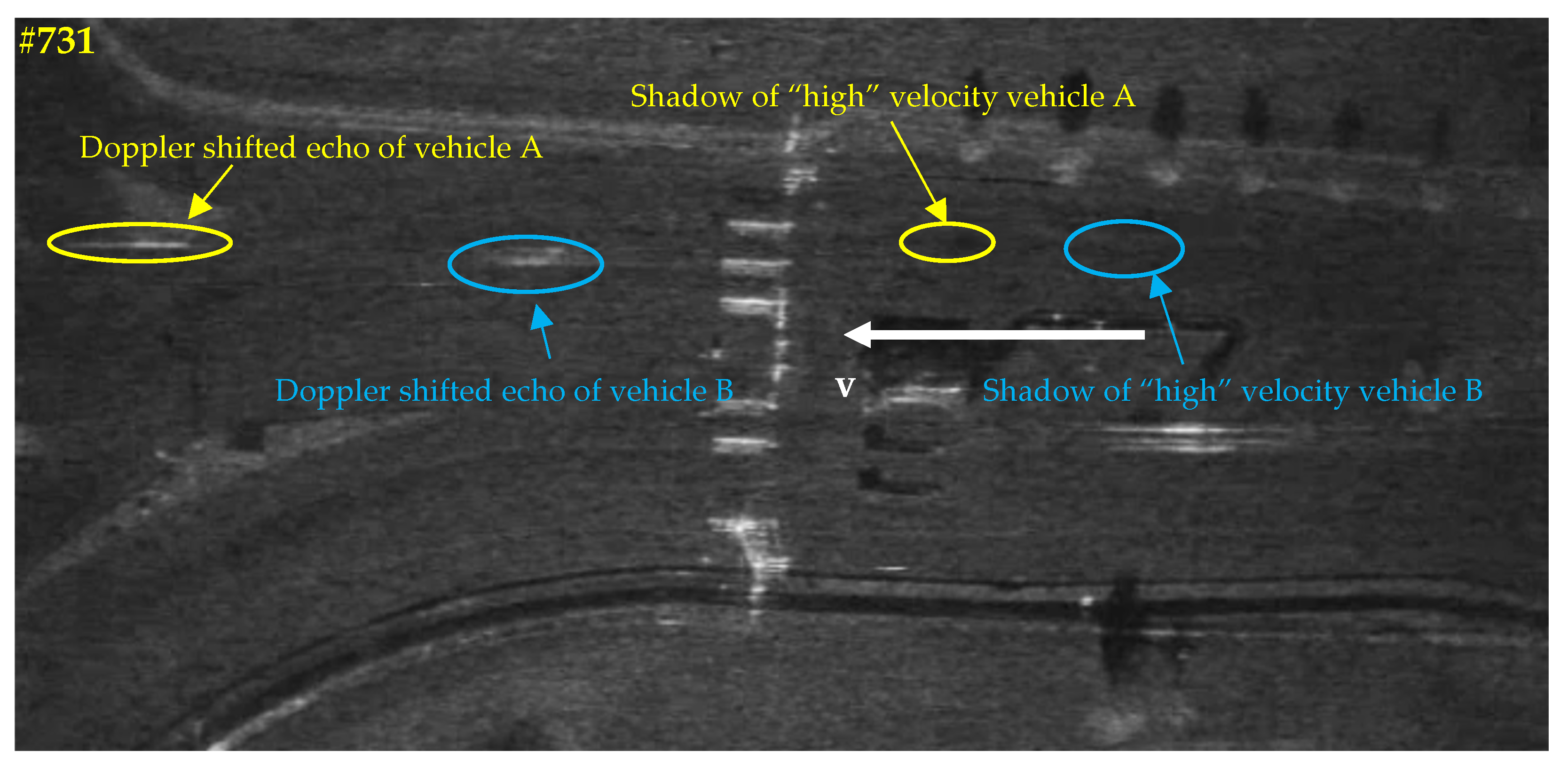
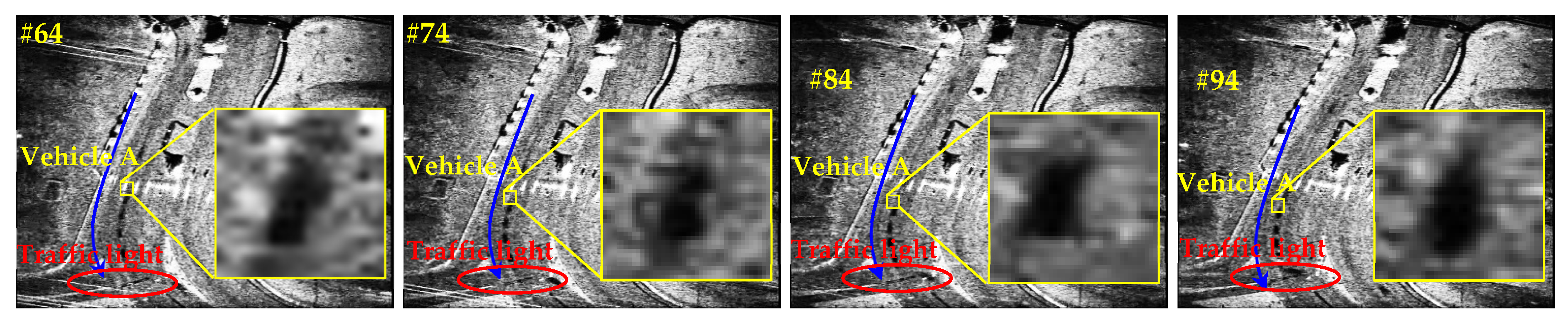
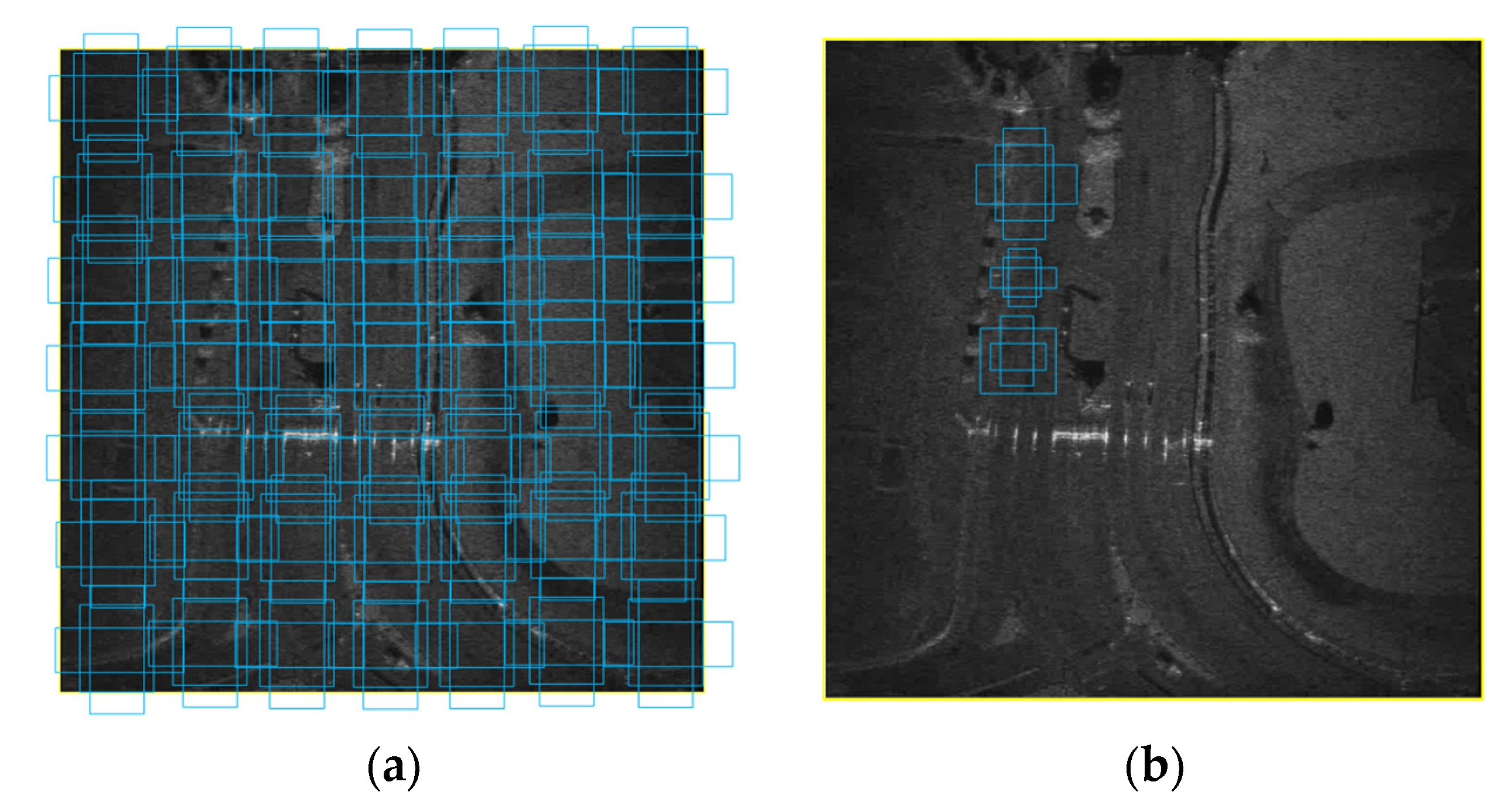
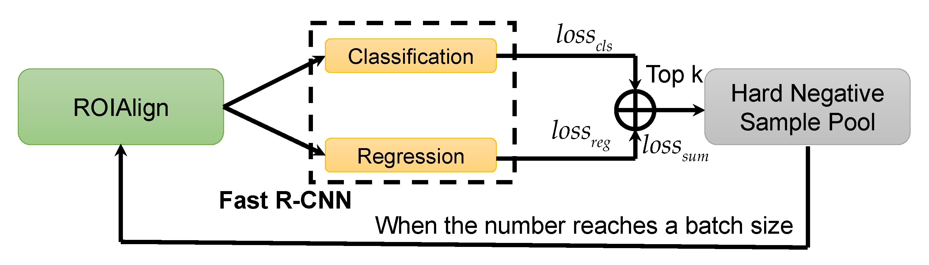
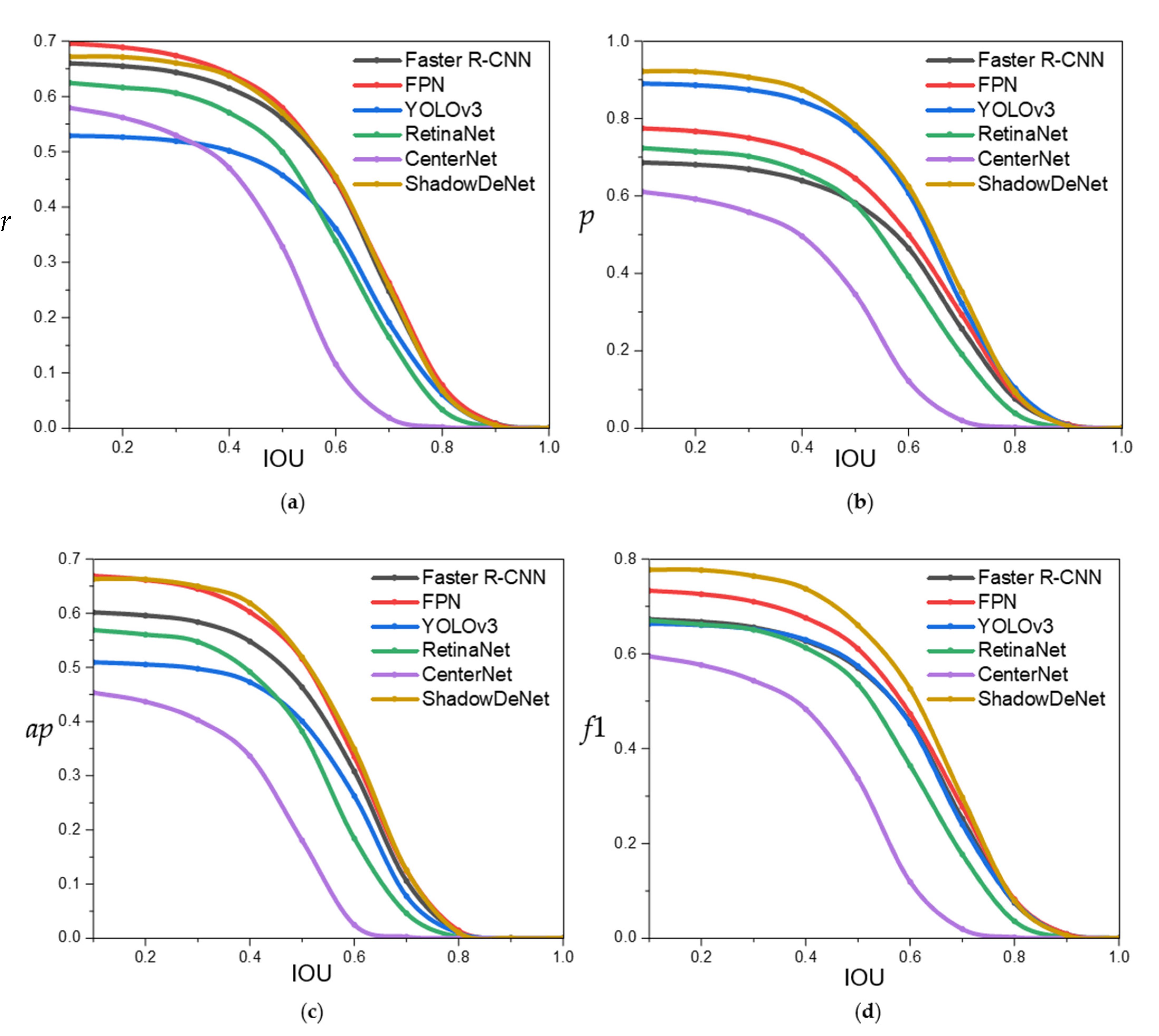
Table 1.
Shadow quality evaluation results with and without HESE. The running time is obtained on the Intel(R) Core(TM) i9-10900KF CPU.
Table 1.
Shadow quality evaluation results with and without HESE. The running time is obtained on the Intel(R) Core(TM) i9-10900KF CPU.
| HESE | Shadow Contrast | Running Time (ms) |
|---|---|---|
| ✗ | 20,979.31 | - |
| √ | 29,215.43 (↑8236.12) | 13.06 |
Table 2.
Radar system parameters of the public Sandia National Laboratories (SNL) video SAR data.
| Parameter | Value |
|---|---|
| Mode | Spotlight |
| Center Frequency | 16.7 GHz (Ku band) |
| Wavelength | 1.8 cm |
| Incidence Angle | 65° |
| Platform Height | 2 km |
| Platform Speed | 245 km/h |
| Cross Range Resolution | 0.1 m |
| Total Imaging Time | 232 s |
| Total Rotation Angle | 200° |
Table 3.
Quantitative results of ShadowDeNet on the SNL video SAR data. #gt: ground truths. #tp: the higher means the better (i.e., correct detections). #fp: the lower means the better (i.e., false alarms). #fn: the lower means the better (i.e., missed detections). r (%): recall, the higher means the better. p (%): precision, the higher means the better. ap (%): average precision, the higher means the better. f1 (%): f1-score, the higher means the better. #: the number.
| HESE 1 | TSAM 2 | SDAL 3 | SGAAL 4 | OHEM 5 | #gt | #tp | #fp | #fn | r (%) | p (%) | ap (%) | f1 (%) |
|---|---|---|---|---|---|---|---|---|---|---|---|---|
| - | - | - | - | - | 1581 | 884 | 636 | 697 | 55.91 | 58.16 | 46.33 | 57.01 |
| √ | 1581 | 898 | 540 | 683 | 56.80 | 62.45 | 49.83 | 59.49 | ||||
| √ | √ | 1581 | 903 | 516 | 678 | 57.12 | 63.64 | 49.84 | 60.20 | |||
| √ | √ | √ | 1581 | 908 | 392 | 673 | 57.43 | 69.85 | 50.91 | 63.03 | ||
| √ | √ | √ | √ | 1581 | 904 | 308 | 677 | 57.18 | 74.59 | 50.33 | 64.73 | |
| √ | √ | √ | √ | √ | 1581 | 902 | 250 | 679 | 57.05 | 78.30 | 51.87 | 66.01 |
| - | - | - | - | - | - | +18 | −386 | −18 | +1.14 | +20.14 | +5.54 | +9.00 |
1 HESE denotes the histogram equalization shadow enhancement. 2 TSAM denotes the transformer self-attention mechanism. 3 SDAL denotes the shape deformation adaptive learning. 4 SGAAL denotes the semantic-guided anchor-adaptive learning. 5 OHEM denotes the online hard example mining.
Table 4.
Performance comparison with the other five state-of-the-art detectors. These detectors have been applied for video SAR moving target shadow detection in the SAR community. The best model is marked in bold. The second-best model is marked by underline. The IOU threshold is 0.50.
Table 4.
Performance comparison with the other five state-of-the-art detectors. These detectors have been applied for video SAR moving target shadow detection in the SAR community. The best model is marked in bold. The second-best model is marked by underline. The IOU threshold is 0.50.
| Method | #gt | #tp | #fp | #fn | r (%) | p (%) | ap (%) | f1 (%) | FPS |
|---|---|---|---|---|---|---|---|---|---|
| Faster R-CNN [25] | 1581 | 884 | 636 | 697 | 55.91 | 58.16 | 46.33 | 57.01 | 15.79 |
| FPN [37] | 1581 | 916 | 504 | 665 | 57.94 | 64.51 | 51.55 | 61.05 | 14.26 |
| YOLOv3 [38] | 1581 | 723 | 216 | 858 | 45.73 | 77.00 | 40.08 | 57.38 | 21.43 |
| RetinaNet [46] | 1581 | 789 | 575 | 792 | 49.91 | 57.84 | 38.19 | 53.58 | 16.67 |
| CenterNet [43,44] | 1581 | 519 | 981 | 1062 | 32.83 | 34.60 | 18.09 | 33.69 | 27.27 |
| ShadowDeNet (Ours) | 1581 | 902 | 250 | 679 | 57.05 | 78.30 | 51.87 | 66.01 | 11.11 |
Table 5.
Quantitative results of ShadowDeNet with and without HESE.
| HESE | #gt | #tp | #fp | #fn | r (%) | p (%) | ap (%) | f1 (%) |
|---|---|---|---|---|---|---|---|---|
| ✗ | 1581 | 868 | 337 | 713 | 54.90 | 72.03 | 49.69 | 62.31 |
| √ | 1581 | 902 | 250 | 679 | 57.05 | 78.30 | 51.87 | 66.01 |
Table 6.
Quantitative results of ShadowDeNet with HESE or AHESE.
| Type | #gt | #tp | #fp | #fn | r (%) | p (%) | ap (%) | f1 (%) |
|---|---|---|---|---|---|---|---|---|
| AHESE | 1581 | 937 | 371 | 644 | 59.27 | 71.64 | 53.33 | 64.87 |
| HESE | 1581 | 902 | 250 | 679 | 57.05 | 78.30 | 51.87 | 66.01 |
Table 7.
Quantitative results of ShadowDeNet with and without TSAM.
| TSAM | #gt | #tp | #fp | #fn | r (%) | p (%) | ap (%) | f1 (%) |
|---|---|---|---|---|---|---|---|---|
| ✗ | 1581 | 891 | 366 | 690 | 56.36 | 70.88 | 49.83 | 62.79 |
| √ | 1581 | 902 | 250 | 679 | 57.05 | 78.30 | 51.87 | 66.01 |
Table 8.
Quantitative results of ShadowDeNet with and without SDAL.
| SDAL | #gt | #tp | #fp | #fn | r (%) | p (%) | ap (%) | f1 (%) |
|---|---|---|---|---|---|---|---|---|
| ✗ | 1581 | 934 | 488 | 647 | 59.08 | 65.68 | 50.33 | 62.20 |
| √ | 1581 | 902 | 250 | 679 | 57.05 | 78.30 | 51.87 | 66.01 |
Table 9.
Quantitative results of ShadowDeNet with and without SGAAL.
| SGAAL | #gt | #tp | #fp | #fn | r (%) | p (%) | ap (%) | f1 (%) |
|---|---|---|---|---|---|---|---|---|
| ✗ | 1581 | 856 | 270 | 725 | 54.14 | 76.02 | 48.68 | 63.24 |
| √ | 1581 | 902 | 250 | 679 | 57.05 | 78.30 | 51.87 | 66.01 |
Table 10.
Quantitative results of ShadowDeNet with different location filter thresholds.
| εL | #gt | #tp | #fp | #fn | r (%) | p (%) | ap (%) | f1 (%) |
|---|---|---|---|---|---|---|---|---|
| 0.00 | 1581 | 873 | 275 | 708 | 55.22 | 76.05 | 48.82 | 63.98 |
| 0.01 | 1581 | 902 | 250 | 679 | 57.05 | 78.30 | 51.87 | 66.01 |
| 0.02 | 1581 | 922 | 381 | 659 | 58.32 | 70.76 | 52.02 | 63.94 |
| 0.03 | 1581 | 893 | 386 | 688 | 56.48 | 69.82 | 49.72 | 62.45 |
| 0.04 | 1581 | 869 | 343 | 712 | 54.97 | 71.70 | 49.02 | 62.23 |
| 0.05 | 1581 | 860 | 326 | 721 | 54.40 | 72.51 | 47.24 | 62.16 |
Table 11.
Quantitative results of ShadowDeNet with and without OHEM.
| OHEM | #gt | #tp | #fp | #fn | r (%) | p (%) | ap (%) | f1 (%) |
|---|---|---|---|---|---|---|---|---|
| ✗ | 1581 | 904 | 308 | 677 | 57.18 | 74.59 | 50.33 | 64.73 |
| √ | 1581 | 902 | 250 | 679 | 57.05 | 78.30 | 51.87 | 66.01 |
Table 12.
Quantitative results of ShadowDeNet on the CASIC 23 research institute video SAR data.
| #gt | #tp | #fp | #fn | r (%) | p (%) | ap (%) | f1 (%) |
|---|---|---|---|---|---|---|---|
| 521 | 286 | 56 | 235 | 54.89 | 83.63 | 52.39 | 66.28 |
Publisher’s Note: MDPI stays neutral with regard to jurisdictional claims in published maps and institutional affiliations. |
© 2022 by the authors. Licensee MDPI, Basel, Switzerland. This article is an open access article distributed under the terms and conditions of the Creative Commons Attribution (CC BY) license (https://creativecommons.org/licenses/by/4.0/).
Share and Cite
MDPI and ACS Style
Bao, J.; Zhang, X.; Zhang, T.; Xu, X. ShadowDeNet: A Moving Target Shadow Detection Network for Video SAR. Remote Sens. 2022, 14, 320. https://0-doi-org.brum.beds.ac.uk/10.3390/rs14020320
AMA Style
Bao J, Zhang X, Zhang T, Xu X. ShadowDeNet: A Moving Target Shadow Detection Network for Video SAR. Remote Sensing. 2022; 14(2):320. https://0-doi-org.brum.beds.ac.uk/10.3390/rs14020320
Chicago/Turabian StyleBao, Jinyu, Xiaoling Zhang, Tianwen Zhang, and Xiaowo Xu. 2022. "ShadowDeNet: A Moving Target Shadow Detection Network for Video SAR" Remote Sensing 14, no. 2: 320. https://0-doi-org.brum.beds.ac.uk/10.3390/rs14020320
Note that from the first issue of 2016, this journal uses article numbers instead of page numbers. See further details here.