Article

Comparative Study of Convolutional Neural Network and Conventional Machine Learning Methods for Landslide Susceptibility Mapping

1
College of Geophysics, Chengdu University of Technology, Chengdu 610059, China
2
Key Laboratory of Earth Exploration and Information Technology of Ministry of Education, Chengdu University of Technology, Chengdu 610059, China
3
National Institute of Natural Hazards, Ministry of Emergency Management of China, Beijing 100085, China
4
The Institute of Exploration Technology of Chinese Academy of Geological Science, Chengdu 611734, China
5
University of Chinese Academy of Sciences, Beijing 100049, China
6
State Key Laboratory of Resources and Environmental Information System, Institute of Geographic Sciences and Natural Resources Research, Chinese Academy of Sciences, Beijing 100101, China
*
Author to whom correspondence should be addressed.
Submission received: 23 November 2021 / Revised: 5 January 2022 / Accepted: 6 January 2022 / Published: 11 January 2022
(This article belongs to the Special Issue Remote Sensing for Landslide Monitoring, Mapping and Modeling)

Abstract

:
Landslide susceptibility mapping (LSM) is a useful tool to estimate the probability of landslide occurrence, providing a scientific basis for natural hazards prevention, land use planning, and economic development in landslide-prone areas. To date, a large number of machine learning methods have been applied to LSM, and recently the advanced convolutional neural network (CNN) has been gradually adopted to enhance the prediction accuracy of LSM. The objective of this study is to introduce a CNN-based model in LSM and systematically compare its overall performance with the conventional machine learning models of random forest, logistic regression, and support vector machine. Herein, we selected Zhangzha Town in Sichuan Province, China, and Lantau Island in Hong Kong, China, as the study areas. Each landslide inventory and corresponding predisposing factors were stacked to form spatial datasets for LSM. The receiver operating characteristic analysis, area under the curve (AUC), and several statistical metrics, such as accuracy, root mean square error, Kappa coefficient, sensitivity, and specificity, were used to evaluate the performance of the models. Finally, the trained models were calculated, and the landslide susceptibility zones were mapped. Results suggest that both CNN and conventional machine learning-based models have a satisfactory performance. The CNN-based model exhibits an excellent prediction capability and achieves the highest performance but also significantly reduces the salt-of-pepper effect, which indicates its great potential for application to LSM.

Graphical Abstract

1. Introduction

Landslides are one of the most serious hazards and are driven by geomorphology, geology, hydrology, and human activities [1]. Heavy rainfall, earthquake, and anthropogenic activities can directly trigger catastrophic landslides. A review by Rawshan et al. [2] mentioned that more intense landslides would happen under the background of the increasingly extreme weather events associated with climate change. When a large landslide occurs, substantial casualties and infrastructure destruction can be caused. The prediction and management of landslides are thus necessary to prevent and mitigate the losses caused by such a hazard. However, due to the lack of reliable precursory data, it is generally difficult to predict landslides in real-time at a good precision, i.e., forecasting their time, place, and magnitude. Another method similar to the landslide prediction is susceptibility mapping, which predicts “where” landslides are more likely to occur in the future [1]. “Susceptibility” means the likelihood of landslide occurrence in a targeted region on the basis of local conditions and predisposing factors [3]. Different from landslide prediction, landslide susceptibility mapping (LSM) is commonly considered as the first stage in hazard management and can provide a scientific guideline for further disaster management, as it calculates the probability of landslide occurrence and identifies the landslide zone of a specific area.
The association between landslides and their environmental factors is the basis of susceptibility mapping. Previous LSM related studies have summarized some environmental factors contributing to landslides, covering topography, land use and land cover (LULC), precipitation, etc. For example, the typical factor of vegetation cover has been proved to affect the slope stability, as its contribution of increasing slope material cohesion and reducing pore water pressures by transpiration [4,5]; slope aspect exerts impact on the direction of the rainfall and sunshine accumulation, which indirectly contributes to the slope stability [6]. Moreover, the rock properties of the land surface are responsible for the spatial distribution characteristics of landslides, especially the rock hardness. The rock hardness inversely correlates with slope failure. An area where the rock hardness is strong is not susceptible to landslides [7]. Therefore, we can adopt various methods to mine the hidden pattern between landslide instances and corresponding environmental factors, and then leverage this to predict susceptibility accurately.
Over the past years, various methods have been proposed and applied for dealing with LSM, including qualitative and quantitative methods. Qualitative methods are knowledge-driven based methods that are dependent on the experience of a geomorphologist [8,9]. Quantitative methods are gradually replacing these methods. Generally, quantitative methods can be further divided into physical-based approaches and data-driven methods. The former needs to comprehensively consider the conditions of geotechnical soils and rocks around the landslides [10]. The development of GIS technology, statistical algorithms, and machine learning has introduced various powerful data-driven methods for LSM. Among them, the widely used models for LSM include, but are not limited to, analytical hierarchy process [11,12], weight of evidence [13,14], discriminant analyses [15,16], naïve Bayes (NB) [17,18], frequency ratio [19,20], index of entropy [21,22], and multivariate regression [23]. In particular, some of the popular machine learning based-models such as random forest (RF), logistic regression (LR), artificial neural networks (ANN), and support vector machines (SVM) are widely used and have achieved satisfactory results in LSM [24,25,26,27]. In addition, hybrid models integrated by statistical learning algorithms and machine learning provide more options for LSM. These models include, but are not limited to, ANN-fuzzy, fuzzy weight of evidence, EBF-fuzzy logic, adaptive neuro-fuzzy inference system, and rotation forest [22,28].
More recently, in addition to the abovementioned methods, the convolutional neural network (CNN)-based model has been applied to LSM [29,30,31,32,33,34]. As a powerful deep learning technique, CNN has shown excellent performance in image classification and identification. The attractive capability of CNN is that it can automatically extract robust and general features from convolutional layers and pooling layers without excessive parameters [35]. As LSM is essentially a binary problem that mines the relationship between landslide predisposing factors and landslides from the dataset and classifies the corresponding pixels, CNN could also be appropriate for LSM. To the best of our knowledge, according to the dimension of data representation, the current implementation of CNN-based models in the LSM-related literature can be divided into two categories: (1) converting landslide predisposing factors into 1D or 2D datasets to fit the need of the CNN and (2) using 3D datasets for LSM. The 1D or 2D data represents the environmental information of landslide locations and do not exploit the spatial information, while 3D data contain the information of the landslides and their surroundings [34]. A detailed comparison study of these techniques can be found in [33].
However, the literature review shows that previous research focused on comparing machine learning and statistical methods, while only a few studies have attempted to compare the CNN with conventional machine learning methods [36,37,38,39]. To fill the gap, it is necessary to investigate these techniques and make a quantitative-systematic comparison. Comparative study is a common research form in LSM literature, which is designed to explore and compare the different models to realize reliable modeling results [40,41]. In light of this, it is considered meaningful to make a comparative study of CNN and conventional machine learning methods, two types of models with different data organization structures. To best of our knowledge, this work is the first to propose a detailed comparative study on the application of the CNN-based model and conventional machine learning methods in LSM, which could provide an effective guide for researchers studying the susceptibility assessment of natural disasters.
The objective of this study is to introduce a CNN-based model in LSM and systematically compare its overall performance with the conventional machine learning models of random forest, logistic regression, and support vector machine in two typical study areas constrained by the external environment (earthquakes and rainfalls). This work also compares in detail these two types of models in terms of the dataset preparation and model effectiveness. More specifically, three typical machine learning models, i.e., random forest, logistic regression, and support vector machine, are selected as the pairwise comparison. These three models have been proven to have good performance in LSM. Two landslide inventories containing earthquake-triggered landslides and rainfall-induced landslides are fed into the conventional machine learning models in terms of matrix form and fed into a CNN-based model in terms of three-dimension (3D) tensors. A series of indices, including the receiver operating characteristic (ROC), root mean square error (RMSE), accuracy, and Kappa coefficients, are used to perform the model evaluation on the training and testing sets.

2. Study Areas and Data

2.1. Study Areas

There are many triggering factors that contribute to landslide occurrences, such as heavy rainfalls, earthquakes, and anthropogenic activities. Of these, heavy rainfalls and earthquakes are common disasters around the world. In this work, we selected two typical areas, Zhangzha Town and Lantau Island, as study areas that suffer from a catastrophe earthquake and heavy rainfall, respectively.
Zhangzha Town is in Jiuzhaigou county on the eastern edge of the Tibetan Plateau, located in Sichuan Province, southwest China, shown in Figure 1a. This area covers approximately 1353 km2 spanning 103°38′E and 104°40′E, and 32°54′N and 33°24′N. Two major geomorphic units, the Tibetan Plateau and the Sichuan Basin, transitioned here and formed a typical valley zone with large undulations and steep slopes. About half of the study area has a slope degree > 30.58°. The majority lithological units are Triassic (40%) and Carboniferous (38%). The tectonic activity has led to frequent earthquakes here. A total of 49 earthquakes with Mw > 5.0 have occurred around the region in the last 100 years [42]. The latest one was the 8 August 2017 Mw 6.5 Jiuzhaigou Earthquake, triggering a large number of co-seismic landslides. These landslides caused severe damage to the natural landscape and disruption to the local traffic.
Lantau Island is the largest outlying island located at the southwest of Hong Kong SAR, covering an area of around 147 km2. As shown in Figure 1b, the undulating and steep terrain occupies most of the area of the island, while there is a small amount of flat ground along the coastline, which makes the majority of the area exposed to certain landslide risks. Meanwhile, Lantau Island enjoys a subtropical monsoon climate that is warm and dry in winter and hot and humid in summer, accompanied by high annual average precipitation, frequent high-intensity storms, and typhoons [43]. Under the combined influence of topography and climate, Lantau Island is thus a landslide-prone area, attracting researchers’ attention. Moreover, the HK international Airport and Disneyland Resort on Lantau Island accept tourists from all over the world every year, which has aroused the concern of the authorities for landslide hazard prevention.

2.2. Landslide Inventories

Landslide inventory is fundamental to the research of landslide susceptibility. A complete landslide inventory map (LIM) records the location, size, and distribution of landslides, which can serve as basic data for further landslide studies.
Tian et al. [44] established a co-seismic landslide inventory around the epicenter of the 2017 Jiuzhaigou earthquake. In their work, a series of high-resolution images before and after the earthquake close to the seismic origin time, including the pre-seismic images on the Google Earth (GE) platform and 0.5 m resolution Geoeye-1 post-seismic images, were chosen for visual interpretation. Combined with the field investigation, a total of 4834 landslides were identified, dominated by small size rockfalls and debris flow. In these landslides, the largest, smallest, and average area are approximately 236,336.2 m2, 7.7 m2, and 1993.2 m2, respectively. In this work, considering the image resolution and the research purpose, we selected 710 locations from the original landslide inventory. In addition, to ensure that the distribution pattern of the selected landslides was consistent with the original inventory, we used the Subset tool in ArcMap to establish a sub-landslide inventory.
The Geotechnical Engineering Office (GEO), the government of Hong Kong, has established a landslide inventory called the “Enhanced Natural Terrain Landslide Inventory (ENTLI)” that records landslides that occurred from 1974 to 2018. This inventory, compiled by visual interpretation, includes almost all the landslides that have occurred in HK. In this work, we selected only the 2492 landslides that occurred on Lantau Island in 2008 as the training inventory without considering the time variation, thus keeping consistent with Zhangzha Town in terms of the time dimension.
Note that all landslide locations in the two inventories were converted into raster data with a grid size of 30 × 30 m using the nearest neighbor resampling method. Subsequently, we divided each landslide inventory into two groups, including training (70%) and testing (30%) data for the construction and testing of the landslide susceptibility model, respectively. As the landslide susceptibility assessment is a binary classification problem that needs positive and negative samples, non-landslide locations with the same proportion as landslide data were randomly selected to balance the landslide inventory.

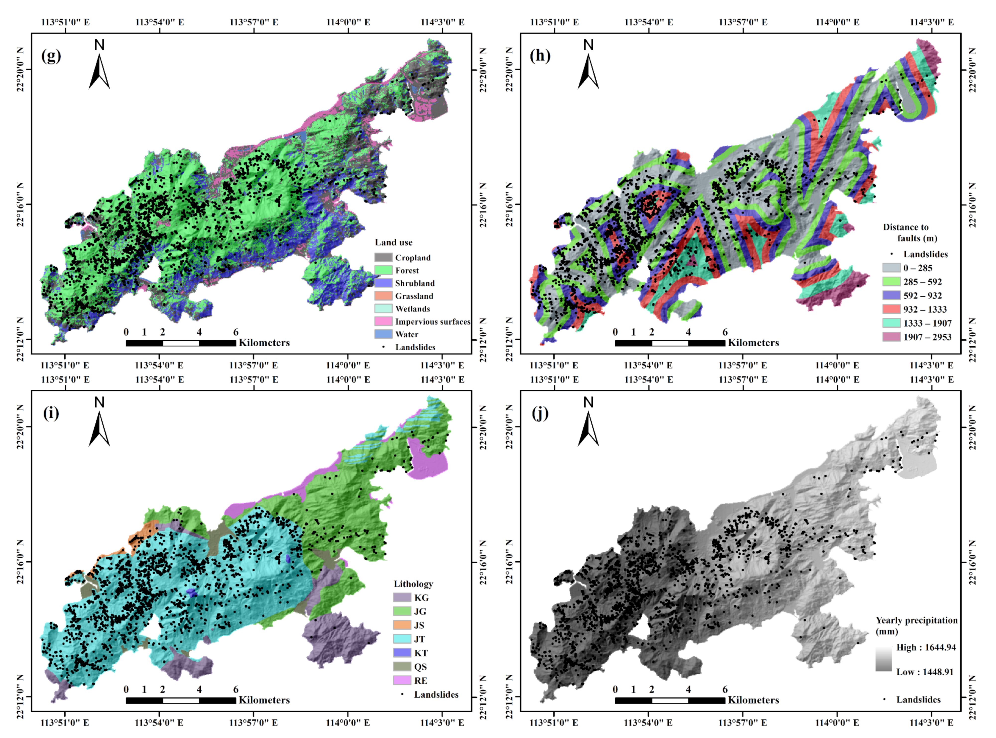
2.3. Landslide Predisposing Factors

The occurrence of landslides is closely related to the combination of various factors, including topography, geology, and other environmental indexes. A proper combination of predisposing factors can make the model more competitive [45]. Because of the complexity of landslides and the diversity of triggering sources, the predisposing factors should be chosen based on the circumstances of the specific area.
In study area of Zhangzha Town, 13 landslide predisposing factors, namely peak ground acceleration (PGA), topographic wetness index (TWI), distance to rivers, distance to roads, distance to faults, normalized difference vegetation index (NDVI), land use, lithology, elevation, slope, aspect, topographic ruggedness index (TRI), and yearly precipitation, were chosen for landslide susceptibility modeling. Table 1 outlines the data source.
PGA is an important indicator of the relationship between co-seismic landslide density and the earthquake and is also a necessary factor in landslide susceptibility mapping [46]. In this study, the PGA data were adapted from USGS (https://earthquake.usgs.gov/) (accessed on 6 November 2021), ranging from 0.12 to 0.26 g and classified into five groups: <0.08, 0.08–0.16, 0.16–0.20, 0.20–0.24, and 0.21–0.26 (Figure 2a). In LSM, TWI is also a frequently-used factor derived from the digital elevation model (DEM) that quantifies topographic control on hydrological processes [47]. As shown in Figure 2b, the TWI used in this work was divided into five categories, with the values of <5.19, 5.19–6.57, 6.57–8.29, 8.29–10.81, 10.81–15.21, and >15.21. The stability of a slope around a river will be significantly affected by the fluctuation of water in the river [48,49]. The roads can affect the spread and size of landslides. Therefore, the distances to rivers and roads derived from a topographical map are considered as predisposing factors (Figure 2c,d). Note that the buffer distance of roads and rivers was determined based on the characteristic of the study area. NDVI is a crucial factor concerned with slope stability, especially in mountain areas. Figure 2e shows that the NDVI is divided into five categories, with values ranging from −0.41 to 0.80. Land use is another common factor contributing to landslides. Using the supervised classification method of the SVM classifier on the Google Earth Engine (GEE), the land use was classified into six categories, namely water, construction land, bare land, dense forests, sparse forests, grass land, and others (Figure 2f). In this study, NDVI and land use were derived from the pre-seismic Sentinel-2 data on the GEE. Geological factors play a significant role in landslide susceptibility, including lithology and distance to faults. The original lithology and faults from a geological map were provided by local authorities with a 1:500,000 scale. The lithology of the study area mainly contains five groups, including Triassic (T1, T2, T3), Carboniferous (C), Quaternary (Q, Qh), Devonian (D), and Permian (P, P2) (Figure 2g). The distance to the faults was generated using a Buffer tool and natural ruptures (Jenks) in ArcMap, which was classified into 0–1992 m, 1992–4276 m, 4276–6795 m, 6495–9665 m, and 9665–14936 m (Figure 2h). Morphological factors including elevation, slope angle, slope aspect, and TRI were derived from the ASTER Global Digital Elevation Model (Figure 2i–l). Precipitation data with the raw resolution 0.04° × 0.04° were downloaded from the Precipitation Estimation from Remotely Sensed Information using Artificial Neural Networks-Dynamic Infrared Rain Rate near real-time (PDIR-Now), developed by the Center for Hydrometeorology and Remote Sensing (CHRS) at the University of California, Irvine (UCI).
For modeling the landslide susceptibility of Lantau Island, ten predisposing factors including elevation, slope aspect, slope angle, TRI, TWI, NDVI, distance to faults, lithology, land use, and yearly precipitation were prepared. The maps of these landslide predisposing factors and more details are provided in Figure A1, Appendix A.
All predisposing factors of Zhangzha Town and Lantau Island were converted into raster data with a grid size of 30 × 30 m, in accordance with the available landslide inventory.

3. Methodology

In the present study, modeling and mapping landslide susceptibility in Zhangzha Town and Lantau Island involve four principal parts: (1) landslide factors selection using information gain ratio (IGR), (2) integrating the landslide inventory and predisposing factors to establish tensor datasets for the CNN-based model and vector datasets for conventional machine learning methods, (3) landslide susceptibility modeling, (4) assessing the predictive capability of models, and (5) mapping the landslide susceptibility of the study areas. A flowchart is shown in Figure 3.
The reason why the CNN module was selected for modeling the landslide susceptibility is that it is capable of capturing high level-features from the data effectively and it can derive other deep learning techniques. Moreover, three typical machine learning models, i.e., random forest, logistic regression, and support vector machine, were selected as the pairwise comparison because these models have been proven to have good performance in LSM.

3.1. Information Gain Ratio

The importance of predisposing factors is associated with their contribution to landslide occurrence. Factors combination that significantly affects the predictability of the susceptibility model is worth discussion. In this work, we used the information gain ratio (IGR) method to quantify the factors’ importance and select optimal combinations before modeling. The IGR values of each factor were calculated via the Weka ver. 3.8.5, an open-source software. The high IGR value of a factor indicates a high prediction ability for modeling and vice versa [50].
Assuming that the training data D consists of n samples (landslide points), and can be divided into the class C i (landslide, non-landslide), then the information entropy of the dataset which is split by class C i can be calculated as
E n t D = i = 1 2 n C i ,   D D log 2 n C i ,   D D
The amount of information gain D 1 , D 2 D m , split from D regarding the predisposing factor P, is estimated as
I n f o G a i n D , P = E n t D   j = 1 m D j D E n t D j
However, the second term of the formula will be a smaller value as the number of factor attribute categories increases, which may reduce the accuracy of the selection. Thus, the information gain ratio was used to estimate the predictive ability of a certain predisposing factor and can be written as
I n f o r a m t i o n g a i n r a t i o D , P = Info G ain D , P S p l i t E n t D , P
where S p l i t E n t quantifies the potential information generated by dividing the training data into m subsets as follows [9]:
S p l i t E n t D , P = j = 1 m D j D log 2 D j D

3.2. Establishment of Spatial Datasets

Having the landslide inventory and predisposing factors, the next step is to format and integrate these data into datasets for further modeling. As shown in Figure 4a, all layers of landslide predisposing factors were stacked together to form a tensor with the size of n × w × h, where n, w, and h represent the number of predisposing factors, the length, and the width of the entire study area, respectively. Then, the specific pixel corresponding to each landslide location was obtained by overlaying the landslide inventory with the factor tensor. Note that the grid size of all the factor layers and the landslide inventory should be the same to ensure that they can be pixel-by-pixel. As mentioned earlier, the grid size of all raster data in this study was 30 × 30 m. However, the factor tensor had different numerical ranges for each dimension. For instance, the slope aspect in Zhangzha Town was divided into nine groups, while PGA was divided into six groups. Therefore, it was essential to normalize each dimension of the factor tensor to improve the machine learning algorithm’s convergent speed and accuracy [51].
Figure 4b shows the landslide and non-landslide locations extracted from the factor tensor used in the deep learning model. The cell corresponding to each landslide location is taken as the center and then expanded into a raster with a size of s × s (this is the window size, and the tuning curves of the parameter are provided in Figure A2, Appendix A). Each cell is assigned a value that contains the data of all the factor layers. In this way, more environmental information around the landslides can be considered for further modeling as opposed to just using one grid [34]. Similarly, the raster of non-landslide location is extracted from the tensor data. The size of the raster used for learning should be set according to specific demands. In this study, the size of the landslide and non-landslide raster was 21 × 21 in Zhangzha Town and 31 × 31 in Lantau Island using the trial-and-error approach. A total of i × 2 (i represents the number of landslides) training and testing tensors with n dimensions extracted from the landslide inventory were generated. Table 2 summarizes the CNN datasets we produced. In this work, the GDAL, a python package (ver. 2.3.2), was adopted to read the raster of each predisposing factor as an editable array. These data were then stacked and expanded via the Numpy package to feed the CNN-based model.
Figure 4c is the diagram of dataset production for the conventional machine learning method. The cell corresponding to each landslide location is extracted from all factor layers and converted to a one-dimensional array with n elements. With the addition of non-landslide sites and the label column, we finally obtain a matrix with a size of all samples × n for learning. The whole process of generating the matrix data was implemented in ArcMap 10.6.

3.3. Convolutional Neural Network (CNN)

The convolutional neural network is perhaps the most popular and widely used deep learning algorithm, composed of three key components: convolutional, down-sampling, and fully connected layers [52]. As the key of CNN, convolutional layers contain multiple convolution kernels that extract finer feature information from the previous layer. Meanwhile, the shared weights strategy in the convolution layer allows the entire network to be trained with fewer parameters than the fully connected network. The down-sampling layer, known as the pooling layer, is leveraged to reduce the size of the feature information as well as to improve the overfitting resistance of the model in the face of different data. The fully connected layer actually acts as a classifier with the same structure as that of the conventional fully connected network. The input of the fully connected layer is the high dimensional features extracted by convolution and pooling operations. Various extended CNN architectures have been proposed and applied in many fields using these basic layers.
As we know, not all landslide predisposing factors contain the same information. That is, the contribution of each predisposing factor to landslide occurrence is different. However, the basic CNN framework assumes that different bands contribute equally. Thus, we added a lightweight channel attention module, namely the squeeze-and-excitation network (SENet), into the pure CNN model. The SENet is capable of calculating the importance of each channel (i.e., landslide predisposing factors) automatically and then, based on the importance, enhancing the important features that are more meaningful to the landslide modeling [53]. The SENet is an embedded network that mainly contains global average pooling, a fully connected layer, as shown in Figure 5, and it can be expressed as follows:
Z = 1 H × W i = 1 H j = 1 W u c i , j
S = F e x Z ,   W = σ g Z , W = σ W 2 R e L U W 1 Z
Z ˜ = F s c a l e Z c , S c = S c · Z c
where Z is the result of the global average pooling operator that converts all factors channel into a 1 × C vector, S is the weighted vector, W 1 R C / r × C , W 2 R C × C / r , r is the scaling parameters, and σ and g represent the Sigmoid and the ReLU function, respectively. Finally, the Z ˜ constrained by the attention mechanism can be obtained by the Z times the inputted data. Note that the embedding of the SENet does not alter the size of each tensor in the pure network and just results in a small extra cost.
In landslide susceptibility mapping, the tensor dataset carrying information on all predisposing factors is input to the convolutional layer. A series of features related to the landslide event is extracted by the convolution operation. Moreover, the pooling layer after the convolutional layer can filter the redundant information. Then, the previous features match the label of input data in the fully connected layer. In the training process, the parameters of CNN are constantly updated with the backpropagation algorithm until an acceptable training accuracy is reached. In this study, the architecture of CNN was designed as shown in Figure 5.
One limitation of the CNN-based model is the setting of its parameters, which takes more time than the conventional machine learning methods. In addition, its code is more complex because of the introduction of the pixel window. Considering the above limitations, the computational efficiency of the CNN-based model is thus lower than that of the conventional machine learning methods. On the other hand, the salt-of-pepper effect that exists in the prediction results could be the limitation of the conventional machine learning methods. A detailed analysis concerning these limitations can be found in Section 5.2 and Section 5.4.

3.4. Conventional Machine Learning Methods

3.4.1. Random Forest

Random forest (RF) is a popular machine learning method introduced by Breiman [54]. It is an ensemble algorithm that generates multiple decision trees with different classification capabilities to learn input data using the bootstrap sampling strategy. The classification is achieved by voting among all the independent decision trees in RF. Different from the single decision tree, the input data of each tree in RF are randomly selected from all input datasets. Each node is split using the subset of predictive features (i.e., landslide predisposing factors) that are randomly selected [55]. In such a way, RF increases diversity among the decision trees and improves the capability to handle the redundant data (over-fitting resistance). Thus, RF is a useful method for mining the useful but hidden association between features and targets within large amounts of data [28].

3.4.2. Logistics Regression

Logistic regression (LR), a generalized linear model, is widely used in mapping landslide susceptibility. In this study, the dependent variable of LR was a binary variable that represented the presence or absence of a landslide (1 means landslide and 0 means non-landslide), and the independent variables were the 12 landslide predisposing factors. The goal of LR is to describe the relationship between binary-coded landslide locations and the various landslide predisposing factors and estimate the probability of landslide occurrence. The general expression of LR is as follows:
z = b 0 + b 1 x 1 + b 2 x 2 + b 3 x 3 + + b n x n
p = 1 1 + e z
where x1, x2, …, xn are the landslide predisposing factors, b0 is the intercept of the model, parameters b1, b2, …, bn are the regression coefficients that must be determined, and p is the probability of landslide occurrence.
In a regression model, the term multicollinearity implies that a perfect linear relationship exists among more than two variables, causing estimates of the model to not be uniquely computed [50]. There is thus a need to implement multicollinearity diagnosis before modeling. The variance inflation factor (VIF) and tolerances methods are commonly used to quantify the multicollinearity among predisposing factors in landslide studies. When the VIF is greater than 10 or the tolerance is smaller than 0.1, there is potential multicollinearity in the datasets [9]. In this work, the abovementioned two indicators of the corresponding landslide datasets in the two study areas are within the expected range, thus implying no potential multicollinearity among landslide predisposing factors.

3.4.3. Support Vector Machine

As a machine learning method based on a structural risk minimization (SRM) strategy, support vector machine (SVM) have been widely used in various classification and regression processes. For the classification of this tool, similar to other algorithms, a boundary needs to be found to delineate the data space. The SVM algorithm achieves the goal of classification by finding a hyperplane with the maximum distance from the classes [56].
Given a training dataset D x i , y i with n samples, where x i R n and the labels y i 1 , 1 , a separating hyperplane is defined as
w   ·   x + b = 0
where w is the coefficient vector that determines the direction of the hyperplane, and b is generally referred to as the bias. Parameters w and b affect the hyperplane synthetically. The optimization of w and b can be considered as a quadratic programming problem:
m i n   w 2 2 + C i = 1 l ξ i
s .   t .   y i w   ·   x i + b 1 ξ i ,   ξ i 0
where C is the penalty, ξ i is the slack factor used for the soft-margin classifier, and l is the number of support vectors. The optimal hyperplane is determined after solving the optimization problem with the Lagrange multiplier a i . The classification function is expressed as
f x   = sgn i = 1 l a i y i x i + b
For nonlinear classification, it is common to use nonlinear kernels to map data in a high-dimensional feature space and then classify it using a separating hyperplane. By introducing kernel functions, Equation (13) becomes
f x = sgn i = 1 l a i y i K x i   ·   x + b
In this study, the radial basis kernel was chosen to be the kernel function K x i   ·   x as
K x i   ·   x   = exp γ || x i x || 2

3.5. Generation of Landslide Susceptibility Maps

According to previous studies, there are two main approaches to generate landslide susceptibility maps (LSM). One is first to calculate the susceptibility values of random points in the study area and then perform inverse distance weighted (IDW) spatial interpolation, which is an effective method to assign values to the entire area using limited points. Then, the landslide susceptibility values are classified into various risk levels using the natural breaking method. Another approach is to calculate the susceptibility values of all pixels of the study area and then classify the values into five risk levels: very low, low, moderate, high, and very high [16]. The choice between random point-based and pixel-based methods is driven primarily by the considerations of study area size and computer performance. An LSM generated by these methods can reflect the distribution of potential landslide hazards with corresponding probability. However, the pixel-based LSM may require more computer resources and code to implement when the study area is large. In this study, the pixel-based method was used to generate landslide susceptibility maps. The GDAL transformed each pixel assigned the predicted value into the raster data with the same coordinate system and spatial resolution as the actual study area.

3.6. Model Performance Evaluation

This study overlaps landslide locations with the landslide susceptibility map for model evaluation. The receiver operating characteristic (ROC) curve is considered an effective metric for assessing the performance of predictive models, specially developed for classification. A ROC curve is a graph with two axes corresponding to “1-specificity” and “sensitivity”. Specificity is the proportion of landslide pixels that are correctly predicted as landslides, Sensitivity is the proportion of non-landslide pixels that are correctly predicted as non-landslide [55]. The area under the curve of ROC indicated by the value of area under the curve (AUC) [57] is another index to test the model performance. The AUC values are between 0.5 and 1. A larger value of AUC generally indicates that the corresponding model can achieve a better performance. In detail, the AUC value can be divided into four levels: poor (0.5–0.6), moderate (0.6–0.7), good (0.7–0.8), and excellent (0.9–1) [58].
Furthermore, several statistical indices, including the root mean square error (RMSE), accuracy, and Kappa index, are adopted for model validation. Generally, a landslide susceptibility model with a lower RMSE value means that it performs better in predicting landslide occurrence. A full description of the Kappa index can be found in the literature [59]. Following are the mathematical expressions of these indices. All metrics were calculated using the metrics class of the Sklearn package:
RMSE   =   Sqrt   1 m i = 1 n y p r e d . y a c t . 2
Accuracy   =   T P + T N T P + T N + F P + F N
Sensitivity   =   T P T P + F N
Specificity   =   T N T N + F P
Kappa   =   P o b s P e x p 1 P e x p
P o b s = T P + T N T S
P e x p = T P + F P × T P + F N + F N + T N × F P + T N T S
Note: Accuracy, sensitivity, and specificity can be derived from the confusion matrix, which is a table presenting the percentages of false positive ( F P ), false negative ( F N ), true positive ( T P ), and true negative ( T N ) observations [60]. In RMSE, y p r e d . and y a c t . represent the predictive and actual values, respectively. In Kappa, TS is the total number of landslide samples in the study area.

4. Results

4.1. Selection of Predisposing Factors

Figure 6 shows the contribution to the landslides of each factor calculated by the information gain ratio (IGR), which was generated by OriginPro 2021. It can be seen that, in the area of Zhangzha Town, the PGA has the highest IGR values of 0.092, while the factors of TWI, yearly precipitation, and slope aspect are less than 0.01, indicating that the weight of these factors is somewhat small. These results reflect the background characteristics of the selected landslide inventory, that is, all samples in the inventory of Zhangzha Town are earthquake-triggered landslides. In return, it could also confirm the accuracy of the prepared data. Interestingly, the weight of yearly precipitation is much less than that of PGA. One explanation for this could be that the strong earthquake ground motion is magnified under the complex topography of Zhangzha Town, exerting a negative impact on the hillslope stability, and this impact is much more significant than that of rainfall [61,62].
Different from the IGR results of Zhangzha Town, the top three factors of Lantau Island are lithology, TRI, and yearly precipitation. The yearly precipitation becomes a governing factor among all factors, while the weight of elevation and related topographic factors are slightly reduced. As described in Section 2.1, Lantau Island suffers from a high annual precipitation, frequent high-intensity storms, and typhoons, thus resulting in the high weight of rainfall.
In addition, the difference in the contribution of factors to landslides between Zhangzha Town and Lantau Island allows us to analyze the generalization ability of the susceptibility models.

4.2. Construction of Models

For the construction of CNN, hyperparameter tuning is the fundamental step to obtain an expected model with high predictability. In this study, the related hyperparameters, including convolutional kernel size, pooling size, loss function, optimizer, epoch, batch size, learning rate, and activation function, were determined using five-fold cross-validation. In terms of the RF, LR, and SVM models, the GridSearchCV method was adopted for parameter tuning [63].
In the training process, the CNN operation on the dataset is as follows: the tensor datasets containing comprehensive environmental information are first fed into two convolutional layers and two down-sampling layers for convolution and pooling operations, generating high-level feature maps, then the feature map is flattened into the fully connected layer and matched to the landslide label. Finally, the entire model can learn the pattern of landslide attribution and the surrounding environment. In terms of conventional machine learning methods, the process is to input the landslide factor vector (representing predisposing factors and training samples) into the model and match the landslide label for training.
Figure 7 shows the training process of the CNN-based model, which can be used as an indicator to determine whether the model converges or not. Intuitively, we hold the idea that the training is completed when the loss of model converges (i.e., no significant fluctuations along loss and accuracy curves). It can be observed that, in the area of Zhangzha Town, the model loss shows a large fluctuation before 25 epochs and stabilizes around epoch 35 over time. In terms of the model of the Lantau Island area, its training curves tend to level off from epoch 65. These results demonstrate that the constructed model converged after learning the hidden pattern between predisposing factors and landslides.
We used the register forward hook function of PyTorch to obtain the outputs of each layer and then visualized it using the matplotlib package. Figure 8 shows the feature extraction process of the CNN-based landslide susceptibility model trained on Zhangzha Town. It can be observed that the selected predisposing factors were fed into the network, and then the high-level features were extracted layer by layer through different convolutional operations. Finally, these high-level features reflect the contributions to landslide occurrence gathered at the output layers to generate the probability map of landslide occurrence. That is to say, the trained CNN-based model can leverage all the landslide predisposing factors simultaneously to map the landslide susceptibility.
The neural network and machine learning methods were performed under the Python environment, outside of the GIS software. The CNN and conventional machine learning models were developed by PyTorch 1.9.0 and Sklearn 1.0.1, respectively. The hardware environment of this study was a personal computer with a 6 GB graphic card GTX1660Ti, a 2.6 GHz Intel® Core™ i7-9750H CPU, and 16 GB of RAM.

4.3. Model Comparison

To quantify the robustness and generalization ability of the susceptibility models, we compared each model’s performance on two typical landslide inventories, including earthquake-triggered and rainfall-induced landslides, based on the testing dataset, AUC, and statistic measures. The results are shown in Figure 9 and Table 3. The ROC curves were drawn by OriginPro based on the outputs gained from the metrics function in PyTorch. It can be seen that, in the area of Zhangzha Town, the AUC values vary from 84.65% to 91.23%, and the CNN-based model achieves the highest values (91.23%), followed by RF (89.92%), LR (85.59%), and SVM (84.65%). Notably, the AUC value of the CNN-based model is 6.58% higher than that of SVM. The CNN model has the highest probability of correctly predicting the non-landslide pixels (specificity = 0.86), whereas the RF has the highest probability of correctly predicting landslide pixels as landslides. The Kappa coefficient varies from 0.53 to 0.67, satisfying the strength of agreement given the magnitude proposed by Landis and Koch et al. [64]: 0.4–0.6 and 0.6–1 are moderate and almost perfect, respectively.
For Lantau Island, the CNN-based model has the highest AUC value (92.70%), followed by RF (90.79%), LR (86.45%), and SVM (86.24%). A similar pattern is also observed in terms of accuracy, RMSE, Kappa, sensitivity, and specificity, which indicates a reasonable agreement between the predicted landslides and the real ones.
Overall, the CNN-based model shows a better performance than the three conventional machine learning (ML) models in predicting the landslide susceptibility of the two selected areas. Furthermore, the AUC and statistical measures of the RF model are close to those of the CNN-based model, and the predictive ability of the SVM and LR is significantly similar. All of these susceptibility models achieved an acceptable performance, and the CNN-based model outperformed the other three ML models with the help of its excellent feature extraction predictive ability in the study areas of Zhangzha Town and Lantau Island.

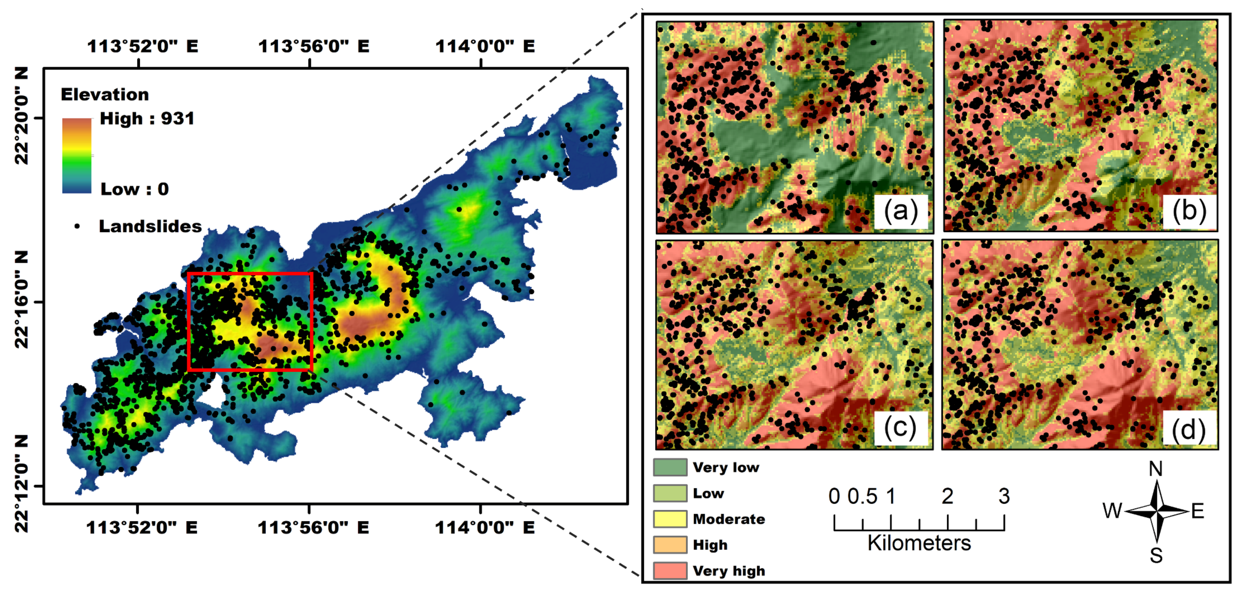
4.4. Landslide Susceptibility Mapping

This study used the CNN, RF, LR, and SVM models to generate the landslide susceptibility maps for Zhangzha Town and Lantau Island (Figure 10 and Figure 11). All pixels in the study area were fed into these trained models for calculating the landslide susceptibility index (LSI). Then, the LSI was divided into five susceptibility levels, namely very low (VLS), low (LS), moderate (MS), high (HS), and very high (VHS), using the natural break approach in ArcMap10.6. The landslide susceptibility zones that indicate the ratio of each susceptibility level to the whole study area were used to analyze the landslide susceptibility maps qualitatively.
In the CNN-based model predicted landslide susceptibility map of the Zhangzha Town, it was observed that the VHS area was relatively concentrated with 13% of the study area, mainly distributed in the middle and northeast, and most landslide points accurately fall into it. A similar spatial distribution of the VHS area was observed in the two conventional ML method models, whereas the VHS and LS areas were lower than those of the CNN-based models, with more than 50% of the area calculated as three susceptibility levels ranging from low to high, as shown in Figure 10 and Figure 12a.
Figure 11 shows the landslide susceptibility map of Lantau Island. It can be observed that the western region of Lantau Island with steep terrain is MS to VHS, while the eastern region is mostly VLS to LS. Additionally, as in the results for Zhangzha Town, a similar tendency regarding the total area of VHS and VLS can be noticed, i.e., the CNN-based model (79%) is significantly higher than RF (55%), SVM (50%), and LR (48%). A landslide susceptibility zone of Lantau Island is shown in Figure 12b.

5. Discussion

Landslide susceptibility mapping (LSM) is a useful tool in predicting the spatial distribution of landslide occurrence. Over the past decades, LSM has gradually evolved from early qualitative analysis to data-driven quantitative methods. The development of machine learning methods in conjunction with the increase of Earth observation data allows us to effectively mine the hidden pattern between landslides and their predisposing factors, which is the basis for susceptibility assessment. Recently, the convolutional neural network (CNN), an effective feature extractor, has been gradually applied to deal with the LSM problem. Compared with the conventional machine learning methods, the CNN-based LSM model is different in many aspects, especially the organization form of the training data and the spatial expression of the predicted results. Taking Zhangzha Town and Lantau Island as the study areas, the present work compares in detail the differences between the CNN-based model and conventional machine learning models in terms of dataset preparation and model effectiveness. To the best of our knowledge, this work is the first to comprehensively compare these two types of landslide susceptibility models, which adds extra value to the literature of LSM or other natural disasters, such as floods and soil erosion. In this subsection, we further discuss the applicability of the CNN-based model from three perspectives: (1) modeling, (2) result analysis, and (3) limitations.

5.1. Model Parameter Analysis

Exploring the effects of hyperparameters on the accuracy of landslide susceptibility modeling could allow us to understand the optimization process better to expand the application to future research. In this subsection, four important hyperparameters of the CNN model, the neurons in the hidden layer, batch size, activation function, and optimizer (i.e., the optimization algorithm), are selected for discussion. Note that when we analyze a specific parameter, the others were set to their optimal values as obtained by cross-validation, which ensures that the independent effect of the hyperparameter is captured.
Figure 13 shows the impact of the number of hidden layer neurons on the AUC value of the validation dataset. It can be observed that the CNN model of Zhangzha Town reached the highest AUC values when the neuron number was 700, and the worst result with the number of 200. In terms of batch size, a series of batch size from 16 to 256 with the power-of-two step were selected for comparison. The results are presented in Figure 13b, indicating the optimal batch size is 30 and the lowest AUC is associated with a batch size of 64. As can be observed from Figure 13a,b, the best activation function and optimizer for modeling are the ReLU and AdaGrad, respectively.
Moreover, the mean deviation (M.D.) of AUC values of each hyperparameter was calculated to measure its sensitivity to the modeling result. The higher M.D. of a hyperparameter is, the more sensitivity it has to the prediction accuracy. The activation function has the highest M.D. (3.77%), followed by the optimizer (1.24%), batch size (1.19%), and neurons in the hidden layer (0.57%). In the same way, the conclusion that the M.D. of the optimizer is the highest in the CNN model of Lantau Island was obtained. In light of these results, much more attention should be paid to the tuning of the activation function and the optimizer when constructing the CNN-based landslide susceptibility model in Zhangzha Town and Lantau Island.

5.2. Computational Efficiency

In recent years, machine learning methods have received extensive attention in LSM. In this paper, CNN was applied to generate the LSM, and the comparative analysis results show that the CNN model achieves a more satisfactory performance than conventional machine learning methods. The performance of models is a vital issue as well as the goal of LSM. Nevertheless, the computational efficiency also needs to be considered. In the experiment, we found that although there is a GPU to accelerate the computation, the CNN-based model consumes much more time than conventional machine learning models in both the training and prediction phases. Accordingly, the performance of conventional machine learning methods is acceptable when considering computational efficiency. On the other hand, the CNN-based approach used in this study extends the LSM from the point-based processing to the image-based processing with a greater potential operating space in terms of the model construction. Compared to conventional machine learning methods, the deep learning approach can be more flexible in changing the network and dataset structure to suit the specific condition. For instance, Fang et al. [65] integrated CNN with three conventional machine learning classifiers to assess landslide susceptibility. The features extracted from the convolutional layers were input into the conventional machine learning classifiers and obtained satisfactory results; Yang et al. [30] proposed a hybrid CNN-based landslide susceptibility model for synchronously capturing the spatial information and the correlated features among the environmental variables. Therefore, the decision to use the CNN method or conventional machine learning methods needs to be determined according to the specific conditions such as experimental equipment, model performance, and disaster emergency degree.

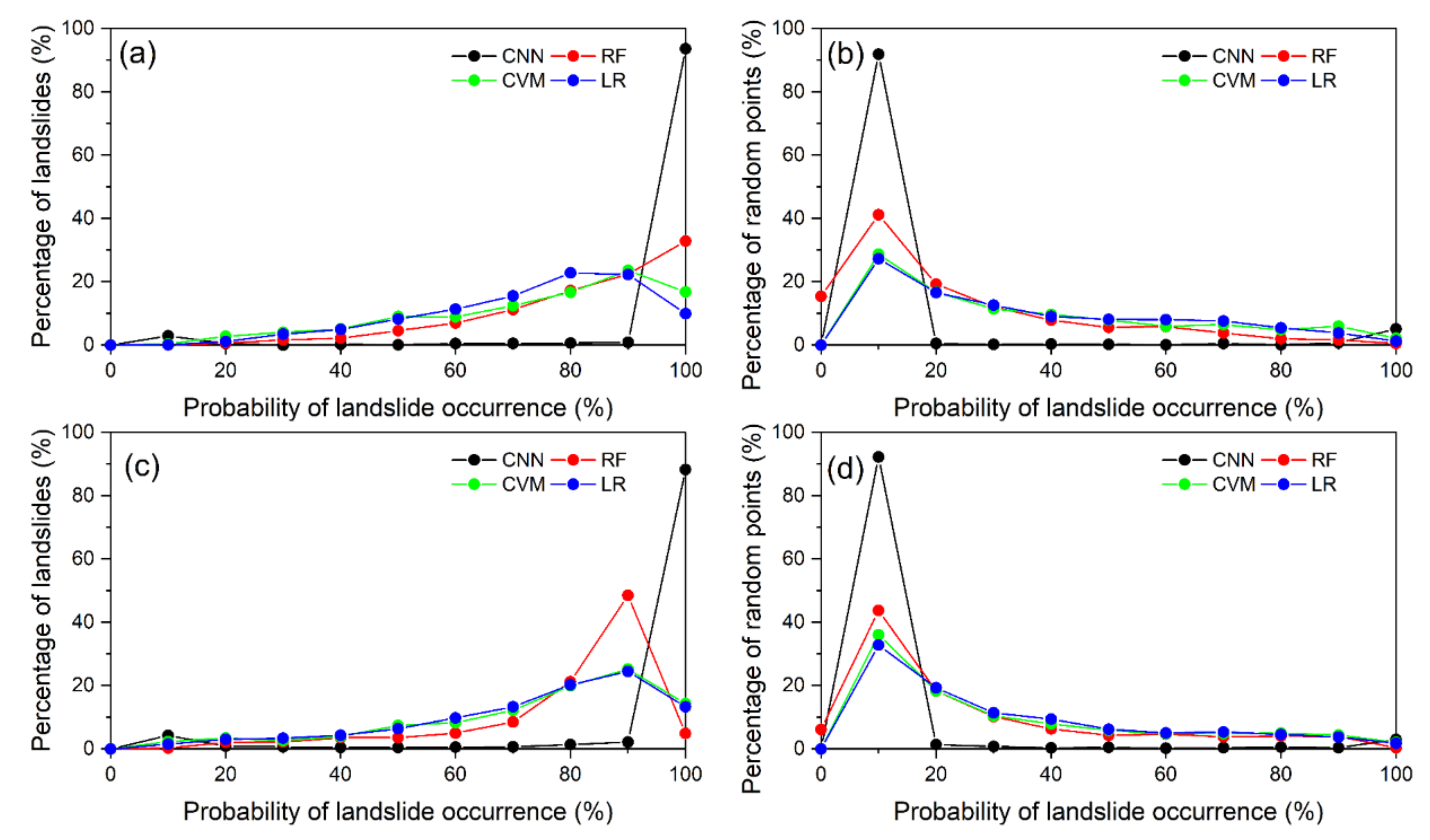
5.3. Reliability Analysis of the Modeling Results

In this work, the performance of the CNN-based model that trained on two study areas is higher than that of the corresponding three benchmark models. However, the ultimate goal of susceptibility mapping is to provide scientific and practical advice on disaster reduction for the civil protection department, rather than simply improving the modeling accuracy. The time cost is a significant issue in disaster prevention and management, which is also suitable in LSM [66]. Note that this time cost refers to the time it takes to determine the target area based on the predicted results, not the modeling time. An ideal landslide susceptibility model is capable of predicting the extreme values of very low and very high susceptibility areas accurately [67].
Figure 14a,b shows the distribution of all sample points in different probability intervals. It can be observed that most of the landslide points and random points (i.e., non-landslide points) are distributed at both ends of the probability interval, and the CNN-based model shows higher sensitivity to the very high and low susceptibility level (i.e., the probability of landslide occurrence is ~1 or ~0). Specifically, the CNN-based model that was trained on Zhangzha Town has the highest percentage of landslides (95%) in the range of the top 20% of the landslide probability, followed by RF (73%) and SVM (57%). On the contrary, most non-landslide points fall in the interval with a lower occurrence probability. Similar distribution curves of Lantau Island can be observed in Figure 14c,d. These results demonstrate that the CNN-based model could better identify the very high and very low susceptibility areas, which reasonably allows decision-makers to focus on prevention targets in a disaster perspective view.
Additionally, sensitivity and specificity are two indicators used to quantify the performance of the models for correctly predicting landslides or non-landslide areas. In this work, these two indicators of the CNN-based model are in the satisfactory range and more balanced as compared to the conventional ML models. All this considered, we can assume that the prediction results of the CNN-based model are reliable and more in line with the view of landslide risk management.

5.4. Analysis of the Salt-and-Pepper Effect in LSM

The salt-and-pepper effect often appears in image segmentation and classification. The reason for this effect is that single pixels with different values cannot form homogeneous areas [68]. Nevertheless, none of the previous studies analyzed the presence of the salt-and-pepper effect in landslide susceptibility maps. The salt-and-pepper in the image segmentation may make the results difficult to distinguish, which for LSM means that this effect may destroy the coherence of the susceptibility assessment in the study area and is not conducive to the subsequent hazards management. Therefore, it is necessary to eliminate the impact of the salt-and-pepper effect in LSM.
Figure 15 shows the landslide susceptibility maps of different models for the same region, demonstrating that the CNN-based model significantly reduces the salt-and-pepper effect compared with the conventional machine learning-based models. A similar result can be observed in Figure A3, Appendix A. The reason for this should be the difference in the establishment of the datasets. As stated in Section 3.2, the training data of the conventional machine learning model consists of single points and the corresponding predisposing factors. However, the CNN training data is expanded with the help of the pixel window, where more pixels are given class labels, and more knowledge is learned by the model, thus creating more homogeneous areas. Therefore, the CNN-based model is more suitable for LSM when considering the salt-and-pepper effect.

5.5. Limitations and Future Research

The results from the CNN-based model trained on the earthquake-triggered and rainfall-induced landslide datasets show that it has the advantages of high prediction ability on testing datasets and achieved the desired accuracy. However, the scale of the case study areas, the limitation of this paper, should be acknowledged. In the case of landslide risk management, the susceptibility assessment is usually conducted at the county level or above. In this study, only a local area of Jiuzhaigou County and an outlying island in Hong Kong were selected as the study areas, and the scale of these two areas is slightly small. As described in Section 5.2, the CNN-based model takes longer to model and predict than conventional machine learning methods; thus, its application to a larger target area may need a trade-off between time efficiency and performance. Therefore, further research of larger-scale areas is required to explore the robustness and reliability of the CNN-based landslide susceptibility model. Another limitation of this study is that the DTM of Lantau Island with a 5 × 5 m grid was resampled to 30 × 30 m for keeping the resolution of all factors consistent, which may have resulted in the loss of some spatial information.
In addition, the framework of landslide susceptibility assessment based on the CNN model can also be applied to landslide polygon recognition in theory. It is worth studying the exact boundary between the two landslide risk reduction techniques.

6. Conclusions

This work compared and analyzed the performance of the CNN-based model and conventional ML models for landslide susceptibility mapping (LSM) in two typical areas, Zhangzha Town and Lantau Island, as study areas that suffer from catastrophe earthquakes and heavy rainfall, respectively. The results demonstrate that the CNN-based model achieved a superior performance over the conventional RF, LR, and SVM models. Moreover, we presented a detailed guide for generating the training datasets for deep learning model-based susceptibility modeling. The following conclusions can be drawn:
  • Among four landslide susceptibility models (i.e., CNN, RF, LR, and SVM), the CNN-based model exhibits the best predictive capability for LSM on the testing datasets.
  • Different from the datasets of conventional ML methods, the 3D dataset allows more spatial information to be considered and learned by CNN-based models. The LSM generated by the CNN-based model is not only sensitive to the high-risk landslide zone but also significantly reduces the salt-and-pepper effect, which guarantees the consistency of susceptibility assessment.
  • Although the CNN-based model achieved significant results, it consumed more time than conventional ML models in both the training and prediction phase. When assessing landslide susceptibility for large areas, time efficiency is an issue that must be considered. Therefore, the choice of the LSM model should be a trade-off between time efficiency and performance.
  • The results of the LSM would assist in disaster management and policy making in the Jiuzhaigou region. Also, this study adds value to the literature of landslide susceptibility mapping through a comparative study of CNN-based and conventional ML models.
Additionally, we only used the typical models and network architecture and did not combine engineering geology analysis methods into the model. In future research, a sophisticated and specific CNN architecture should be designed for dealing with the LSM, which may lead to better performance.

Author Contributions

Conceptualization, R.L. and X.Y.; methodology, R.L. and X.Y.; software, X.Y.; validation, X.Z. and X.Y.; formal analysis, X.Y.; resources, C.X. and L.W.; data curation, C.X. and L.W.; writing—original draft preparation, R.L. and X.Y.; writing—review and editing, R.L., X.Y., C.X., L.W. and X.Z.; visualization, X.Y.; project administration, R.L.; funding acquisition, R.L. All authors have read and agreed to the published version of the manuscript.

Funding

This research was funded by the Bureau of Geology and mineral resources exploration and development of Sichuan Province, grant number 20170612-0413, and The Research Center for Meteorological Disaster Prediction and Early Warning and Emergency Management 2021 General Project, grant number ZHYJ21-YB04.

Data Availability Statement

Landslide inventory data may be available from the corresponding author or the third author upon request. The core code for reading the predisposing factors and label data and generating the pixel window can be found in the GitHub repository: https://github.com/kkshiney/RS_ML_DeepLearning_LSM (accessed on 22 November 2021).

Acknowledgments

The authors would like to thank the handling editors and the four anonymous reviewers for their valuable comments on the earlier version of the manuscript. The authors wish to thank the lab’s staff for their valuable comments and contributions.

Conflicts of Interest

The authors declare no conflict of interest.

Abbreviations

LSM  landslide susceptibility mapping
CNN   convolutional neural network
ML  machine learning
AUC   area under the curve
LULC  land use and land cover
GIS  geographic information system
RF  random forest
ANN   artificial neural network
SVM  support vector machine
1/2/3D  1/2/3 dimension
GEE  Google Earth Engine
IGR  information gain ratio
SENet  squeeze-and-excitation network
ReLU  rectified linear unit
SRM  structure risk minimization
IDW  inverse distance weighted
ROC  receiver operating characteristic
RMSE  root mean square error
LSI  landslide susceptibility index
M.D.  mean deviation

Appendix A

Figure A1. Maps showing landslide predisposing factors in Lantau Island: (a) elevation, (b) slope aspect, (c) slope angle, (d) TRI, (e) TWI, (f) NDVI, (g) land use, (h) distance to faults, (i) lithology, and (j) yearly precipitation.
Remotesensing 14 00321 g0a1aRemotesensing 14 00321 g0a1b
Figure A2. AUC variation of the CNN-based model with different window size.
Remotesensing 14 00321 g0a2
Figure A3. Local magnification of Figure 11 (ad).
Remotesensing 14 00321 g0a3
Table A1. Information of predisposing factors for modeling the Zhangzha Town landslide susceptibility.
Predisposing FactorsData TypeSourceResolution
ElevationRasterEsri China (HK)30 × 30 m
Slope aspect
Slope angle
TRI
TWI
NDVIRasterDerived from Sentinel-2A on the Google Earth Engine10 × 10 m
Land useRasterDerived from the GLC_FCS30 datasets (https://0-doi-org.brum.beds.ac.uk/10.5194/essd-13-2753-2021) (accessed on 6 November 2021)30 × 30 m
Distance to faultsLinesDerived from the geological map supported by the Civil Engineering and Development Department, HKSAR1:100,000
LithologyPolygon
Yearly precipitationRasterPDIR-Now satellite precipitation product4 × 4 km
Table A2. Information of the lithology in Lantau Island.
Symbol Geological Age Main Lithology
KGCretaceousGranitic rocks
JGJurassicGranitic rocks
JSJurassicSandstone, siltstone, and mudstone
JTJurassicTuff and lava
KTCretaceousTuff and lava
QSQuaternarySuperficial deposits (silt, sand, and gravel)
RE-Fill

References

  1. Jaafari, A.; Panahi, M.; Pham, B.T.; Shahabi, H.; Bui, D.T.; Rezaie, F.; Lee, S. Meta optimization of an adaptive neuro-fuzzy inference system with grey wolf optimizer and biogeography-based optimization algorithms for spatial prediction of landslide susceptibility. Catena 2019, 175, 430–445. [Google Scholar] [CrossRef]
  2. Ali, R.; Kuriqi, A.; Kisi, O. Human–Environment Natural Disasters Interconnection in China: A Review. Climate 2020, 8, 48. [Google Scholar] [CrossRef] [Green Version]
  3. Reichenbach, P.; Rossi, M.; Malamud, B.D.; Mihir, M.; Guzzetti, F. A review of statistically-based landslide susceptibility models. Earth-Sci. Rev. 2018, 180, 60–91. [Google Scholar] [CrossRef]
  4. Jones, J.N.; Boulton, S.J.; Bennett, G.L.; Stokes, M.; Whitworth, M.R.Z. Temporal Variations in Landslide Distributions Following Extreme Events: Implications for Landslide Susceptibility Modeling. J. Geophys. Res. Earth Surf. 2021, 126, e2021JF006067. [Google Scholar] [CrossRef]
  5. Sidle, R.C.; Bogaard, T.A. Dynamic earth system and ecological controls of rainfall-initiated landslides. Earth-Sci. Rev. 2016, 159, 275–291. [Google Scholar] [CrossRef]
  6. Youssef, A.M.; Al-Kathery, M.; Pradhan, B. Landslide susceptibility mapping at Al-Hasher area, Jizan (Saudi Arabia) using GIS-based frequency ratio and index of entropy models. Geosci. J. 2014, 19, 113–134. [Google Scholar] [CrossRef]
  7. Yu, X.; Zhang, K.; Song, Y.; Jiang, W.; Zhou, J. Study on landslide susceptibility mapping based on rock-soil characteristic factors. Sci. Rep. 2021, 11, 15476. [Google Scholar] [CrossRef]
  8. Lucà, F.; Conforti, M.; Robustelli, G. Comparison of GIS-based gullying susceptibility mapping using bivariate and multivariate statistics: Northern Calabria, South Italy. Geomorphology 2011, 134, 297–308. [Google Scholar] [CrossRef]
  9. Tien Bui, D.; Tuan, T.A.; Klempe, H.; Pradhan, B.; Revhaug, I. Spatial prediction models for shallow landslide hazards: A comparative assessment of the efficacy of support vector machines, artificial neural networks, kernel logistic regression, and logistic model tree. Landslides 2015, 13, 361–378. [Google Scholar] [CrossRef]
  10. Muceku, Y.; Korini, O.; Kuriqi, A. Geotechnical Analysis of Hill’s Slopes Areas in Heritage Town of Berati, Albania. Period. Polytech. Civ. Eng. 2016, 60, 61–73. [Google Scholar] [CrossRef] [Green Version]
  11. Abedini, M.; Tulabi, S. Assessing LNRF, FR, and AHP models in landslide susceptibility mapping index: A comparative study of Nojian watershed in Lorestan province, Iran. Environ. Earth Sci. 2018, 77, 405. [Google Scholar] [CrossRef]
  12. Pourghasemi, H.R.; Rossi, M. Landslide susceptibility modeling in a landslide prone area in Mazandarn Province, north of Iran: A comparison between GLM, GAM, MARS, and M-AHP methods. Theor. Appl. Climatol. 2016, 130, 609–633. [Google Scholar] [CrossRef]
  13. Dahal, R.K.; Hasegawa, S.; Nonomura, A.; Yamanaka, M.; Masuda, T.; Nishino, K. GIS-based weights-of-evidence modelling of rainfall-induced landslides in small catchments for landslide susceptibility mapping. Environ. Geol. 2007, 54, 311–324. [Google Scholar] [CrossRef]
  14. Hasekioğulları, G.D.; Ercanoglu, M. A new approach to use AHP in landslide susceptibility mapping: A case study at Yenice (Karabuk, NW Turkey). Nat. Hazards 2012, 63, 1157–1179. [Google Scholar] [CrossRef]
  15. Dong, J.-J.; Tung, Y.-H.; Chen, C.-C.; Liao, J.-J.; Pan, Y.-W. Discriminant analysis of the geomorphic characteristics and stability of landslide dams. Geomorphology 2009, 110, 162–171. [Google Scholar] [CrossRef]
  16. He, S.; Pan, P.; Dai, L.; Wang, H.; Liu, J. Application of kernel-based Fisher discriminant analysis to map landslide susceptibility in the Qinggan River delta, Three Gorges, China. Geomorphology 2012, 171, 30–41. [Google Scholar] [CrossRef]
  17. Lee, S.; Lee, M.-J.; Jung, H.-S.; Lee, S. Landslide susceptibility mapping using Naïve Bayes and Bayesian network models in Umyeonsan, Korea. Geocarto Int. 2019, 35, 1665–1679. [Google Scholar] [CrossRef]
  18. Tsangaratos, P.; Ilia, I. Comparison of a logistic regression and Naïve Bayes classifier in landslide susceptibility assessments: The influence of models complexity and training dataset size. Catena 2016, 145, 164–179. [Google Scholar] [CrossRef]
  19. Jana, S.K.; Sekac, T.; Pal, D.K. Geo-spatial approach with frequency ratio method in landslide susceptibility mapping in the Busu River catchment, Papua New Guinea. Spat. Inf. Res. 2018, 27, 49–62. [Google Scholar] [CrossRef]
  20. Yilmaz, I. Landslide susceptibility mapping using frequency ratio, logistic regression, artificial neural networks and their comparison: A case study from Kat landslides (Tokat—Turkey). Comput. Geosci. 2009, 35, 1125–1138. [Google Scholar] [CrossRef]
  21. Constantin, M.; Bednarik, M.; Jurchescu, M.C.; Vlaicu, M. Landslide susceptibility assessment using the bivariate statistical analysis and the index of entropy in the Sibiciu Basin (Romania). Environ. Earth Sci. 2010, 63, 397–406. [Google Scholar] [CrossRef]
  22. Zhang, T.-y.; Han, L.; Zhang, H.; Zhao, Y.-h.; Li, X.-a.; Zhao, L. GIS-based landslide susceptibility mapping using hybrid integration approaches of fractal dimension with index of entropy and support vector machine. J. Mt. Sci. 2019, 16, 1275–1288. [Google Scholar] [CrossRef]
  23. Felicísimo, Á.M.; Cuartero, A.; Remondo, J.; Quirós, E. Mapping landslide susceptibility with logistic regression, multiple adaptive regression splines, classification and regression trees, and maximum entropy methods: A comparative study. Landslides 2012, 10, 175–189. [Google Scholar] [CrossRef]
  24. Hong, H.; Pradhan, B.; Jebur, M.N.; Bui, D.T.; Xu, C.; Akgun, A. Spatial prediction of landslide hazard at the Luxi area (China) using support vector machines. Environ. Earth Sci. 2015, 75, 1–14. [Google Scholar] [CrossRef]
  25. Pourghasemi, H.R.; Kornejady, A.; Kerle, N.; Shabani, F. Investigating the effects of different landslide positioning techniques, landslide partitioning approaches, and presence-absence balances on landslide susceptibility mapping. Catena 2020, 187, 104364. [Google Scholar] [CrossRef]
  26. Zare, M.; Pourghasemi, H.R.; Vafakhah, M.; Pradhan, B. Landslide susceptibility mapping at Vaz Watershed (Iran) using an artificial neural network model: A comparison between multilayer perceptron (MLP) and radial basic function (RBF) algorithms. Arab. J. Geosci. 2012, 6, 2873–2888. [Google Scholar] [CrossRef]
  27. Li, L.; Liu, R.; Pirasteh, S.; Chen, X.; He, L.; Li, J. A novel genetic algorithm for optimization of conditioning factors in shallow translational landslides and susceptibility mapping. Arab. J. Geosci. 2017, 10, 209. [Google Scholar] [CrossRef]
  28. Chen, W.; Peng, J.; Hong, H.; Shahabi, H.; Pradhan, B.; Liu, J.; Zhu, A.X.; Pei, X.; Duan, Z. Landslide susceptibility modelling using GIS-based machine learning techniques for Chongren County, Jiangxi Province, China. Sci. Total Environ. 2018, 626, 1121–1135. [Google Scholar] [CrossRef]
  29. Wei, X.; Zhang, L.; Luo, J.; Liu, D. A hybrid framework integrating physical model and convolutional neural network for regional landslide susceptibility mapping. Nat. Hazards 2021, 109, 471–497. [Google Scholar] [CrossRef]
  30. Yang, X.; Liu, R.; Yang, M.; Chen, J.; Liu, T.; Yang, Y.; Chen, W.; Wang, Y. Incorporating Landslide Spatial Information and Correlated Features among Conditioning Factors for Landslide Susceptibility Mapping. Remote Sens. 2021, 13, 2166. [Google Scholar] [CrossRef]
  31. Thi Ngo, P.T.; Panahi, M.; Khosravi, K.; Ghorbanzadeh, O.; Kariminejad, N.; Cerda, A.; Lee, S. Evaluation of deep learning algorithms for national scale landslide susceptibility mapping of Iran. Geosci. Front. 2021, 12, 505–519. [Google Scholar] [CrossRef]
  32. Sameen, M.I.; Pradhan, B.; Lee, S. Application of convolutional neural networks featuring Bayesian optimization for landslide susceptibility assessment. Catena 2020, 186, 104249. [Google Scholar] [CrossRef]
  33. Wang, Y.; Fang, Z.; Hong, H. Comparison of convolutional neural networks for landslide susceptibility mapping in Yanshan County, China. Sci. Total Environ. 2019, 666, 975–993. [Google Scholar] [CrossRef]
  34. Yi, Y.; Zhang, Z.; Zhang, W.; Jia, H.; Zhang, J. Landslide susceptibility mapping using multiscale sampling strategy and convolutional neural network: A case study in Jiuzhaigou region. Catena 2020, 195, 104851. [Google Scholar] [CrossRef]
  35. Zhao, W.; Du, S.; Emery, W.J. Object-Based Convolutional Neural Network for High-Resolution Imagery Classification. IEEE J. Sel. Top. Appl. Earth Obs. Remote Sens. 2017, 10, 3386–3396. [Google Scholar] [CrossRef]
  36. Chen, T.; Zhu, L.; Niu, R.-q.; Trinder, C.J.; Peng, L.; Lei, T. Mapping landslide susceptibility at the Three Gorges Reservoir, China, using gradient boosting decision tree, random forest and information value models. J. Mt. Sci. 2020, 17, 670–685. [Google Scholar] [CrossRef]
  37. Chen, W.; Zhang, S. GIS-based comparative study of Bayes network, Hoeffding tree and logistic model tree for landslide susceptibility modeling. Catena 2021, 203, 105344. [Google Scholar] [CrossRef]
  38. Barella, C.F.; Sobreira, F.G.; Zêzere, J.L. A comparative analysis of statistical landslide susceptibility mapping in the southeast region of Minas Gerais state, Brazil. Bull. Eng. Geol. Environ. 2018, 78, 3205–3221. [Google Scholar] [CrossRef]
  39. Wang, Y.; Fang, Z.; Wang, M.; Peng, L.; Hong, H. Comparative study of landslide susceptibility mapping with different recurrent neural networks. Comput. Geosci. 2020, 138, 104445. [Google Scholar] [CrossRef]
  40. Huang, F.; Ye, Z.; Jiang, S.-H.; Huang, J.; Chang, Z.; Chen, J. Uncertainty study of landslide susceptibility prediction considering the different attribute interval numbers of environmental factors and different data-based models. Catena 2021, 202, 105250. [Google Scholar] [CrossRef]
  41. Liu, R.; Li, L.; Pirasteh, S.; Lai, Z.; Yang, X.; Shahabi, H. The performance quality of LR, SVM, and RF for earthquake-induced landslides susceptibility mapping incorporating remote sensing imagery. Arab. J. Geosci. 2021, 14, 1–15. [Google Scholar] [CrossRef]
  42. Lanxin, D.A.I.; Qiang, X.U.; Xuanmei, F.A.N.; Ming, C.H.A.N.G.; Qin, Y.A.N.G.; Fan, Y.A.N.G.; Jing, R.E.N. A preliminary study on spatial distribution patterns of landslides triggered by Jiuzhaigou earthquake in Sichuan on August 8th, 2017 and their susceptibility assessment. J. Eng. Geol. 2017, 25, 1151–1164. [Google Scholar] [CrossRef]
  43. Wang, H.; Zhang, L.; Yin, K.; Luo, H.; Li, J. Landslide identification using machine learning. Geosci. Front. 2021, 12, 351–364. [Google Scholar] [CrossRef]
  44. Tian, Y.; Xu, C.; Ma, S.; Xu, X.; Wang, S.; Zhang, H. Inventory and Spatial Distribution of Landslides Triggered by the 8th August 2017 MW 6.5 Jiuzhaigou Earthquake, China. J. Earth Sci. 2018, 30, 206–217. [Google Scholar] [CrossRef]
  45. Chen, X.; Chen, W. GIS-based landslide susceptibility assessment using optimized hybrid machine learning methods. Catena 2021, 196, 104833. [Google Scholar] [CrossRef]
  46. Meunier, P.; Hovius, N.; Haines, A.J. Regional patterns of earthquake-triggered landslides and their relation to ground motion. Geophys. Res. Lett. 2007, 34, L20408. [Google Scholar] [CrossRef] [Green Version]
  47. Sørensen, R.; Zinko, U.; Seibert, J. On the calculation of the topographic wetness index: Evaluation of different methods based on field observations. Hydrol. Earth Syst. Sci. 2006, 10, 101–112. [Google Scholar] [CrossRef] [Green Version]
  48. Cevik, E.; Topal, T. GIS-based landslide susceptibility mapping for a problematic segment of the natural gas pipeline, Hendek (Turkey). Environ. Geol. 2003, 44, 949–962. [Google Scholar] [CrossRef]
  49. Saha, A.K.; Gupta, R.P.; Arora, M.K. GIS-based Landslide Hazard Zonation in the Bhagirathi (Ganga) Valley, Himalayas. Int. J. Remote Sens. 2010, 23, 357–369. [Google Scholar] [CrossRef]
  50. Ozdemir, A.; Altural, T. A comparative study of frequency ratio, weights of evidence and logistic regression methods for landslide susceptibility mapping: Sultan Mountains, SW Turkey. J. Asian Earth Sci. 2013, 64, 180–197. [Google Scholar] [CrossRef]
  51. James, G.; Witten, D.; Hastie, T.; Tibshirani, R. An Introduction to Statistical Learning; Springer: New York, NY, USA, 2013. [Google Scholar]
  52. Ye, C.-m.; Liu, X.; Xu, H.; Ren, S.-c.; Li, Y.; Li, J. Classification of hyperspectral images based on a convolutional neural network and spectral sensitivity. J. Zhejiang Univ.-Sci. A 2020, 21, 240–248. [Google Scholar] [CrossRef]
  53. Tang, P.; Du, P.; Xia, J.; Zhang, P.; Zhang, W. Channel Attention-Based Temporal Convolutional Network for Satellite Image Time Series Classification. IEEE Geosci. Remote Sens. Lett. 2021, 19, 1–5. [Google Scholar] [CrossRef]
  54. Breiman, L. Random forests. Mach. Learn. 2001, 45, 5–32. [Google Scholar] [CrossRef] [Green Version]
  55. Youssef, A.M.; Pourghasemi, H.R.; Pourtaghi, Z.S.; Al-Katheeri, M.M. Landslide susceptibility mapping using random forest, boosted regression tree, classification and regression tree, and general linear models and comparison of their performance at Wadi Tayyah Basin, Asir Region, Saudi Arabia. Landslides 2015, 13, 839–856. [Google Scholar] [CrossRef]
  56. Cortes, C.; Vapnik, V. Support-vector networks. Mach. Learn. 1995, 20, 273–297. [Google Scholar] [CrossRef]
  57. Schneider, M.J.; Gorr, W.L. ROC-based model estimation for forecasting large changes in demand. Int. J. Forecast. 2015, 31, 253–262. [Google Scholar] [CrossRef] [Green Version]
  58. Wu, Y.; Ke, Y.; Chen, Z.; Liang, S.; Zhao, H.; Hong, H. Application of alternating decision tree with AdaBoost and bagging ensembles for landslide susceptibility mapping. Catena 2020, 187, 104396. [Google Scholar] [CrossRef]
  59. Cohen, J. A Coefficient of Agreement for Nominal Scales. Educ. Psychol. Meas. 1960, 20, 37–46. [Google Scholar] [CrossRef]
  60. Chen, H.X.; Zhang, L.M. A physically-based distributed cell model for predicting regional rainfall-induced shallow slope failures. Eng. Geol. 2014, 176, 79–92. [Google Scholar] [CrossRef]
  61. Meunier, P.; Hovius, N.; Haines, J.A. Topographic site effects and the location of earthquake induced landslides. Earth Planet. Sci. Lett. 2008, 275, 221–232. [Google Scholar] [CrossRef]
  62. Brain, M.J.; Rosser, N.J.; Tunstall, N. The control of earthquake sequences on hillslope stability. Geophys. Res. Lett. 2017, 44, 865–872. [Google Scholar] [CrossRef] [Green Version]
  63. Cao, J.; Zhang, Z.; Du, J.; Zhang, L.; Song, Y.; Sun, G. Multi-geohazards susceptibility mapping based on machine learning—A case study in Jiuzhaigou, China. Nat. Hazards 2020, 102, 851–871. [Google Scholar] [CrossRef]
  64. Landis, J.R.; Koch, G.G. The Measurement of Observer Agreement for Categorical Data. Biometrics 1977, 33, 159–174. [Google Scholar] [CrossRef] [PubMed] [Green Version]
  65. Fang, Z.; Wang, Y.; Peng, L.; Hong, H. Integration of convolutional neural network and conventional machine learning classifiers for landslide susceptibility mapping. Comput. Geosci. 2020, 139, 104470. [Google Scholar] [CrossRef]
  66. Cantarino, I.; Carrion, M.A.; Goerlich, F.; Martinez Ibañez, V. A ROC analysis-based classification method for landslide susceptibility maps. Landslides 2018, 16, 265–282. [Google Scholar] [CrossRef]
  67. Guo, Z.; Shi, Y.; Huang, F.; Fan, X.; Huang, J. Landslide susceptibility zonation method based on C5.0 decision tree and K-means cluster algorithms to improve the efficiency of risk management. Geosci. Front. 2021, 12, 101249. [Google Scholar] [CrossRef]
  68. Blaschke, T.; Lang, S.; Lorup, E.; Strobl, J.; Zeil, P. Object-Oriented Image Processing in an Integrated GIS/Remote Sensing Environment and Perspectives for Environmental Applications. Environ. Inf. Plan. Politics Public 2000, 2, 555–570. [Google Scholar]
Figure 1. Location of the study areas: (a) Zhangzha Town and (b) Lantau Island.
Remotesensing 14 00321 g001
Figure 2. Maps showing landslide predisposing factors used in Zhangzha Town: (a) PGA, (b) TWI, (c) distance to rivers, (d) distance to roads, (e) NDVI, (f) land use, (g) lithology, (h) distance to faults, (i) elevation, (j) slope angle, (k) slope aspect, (l) TRI, and (m) yearly precipitation.
Remotesensing 14 00321 g002aRemotesensing 14 00321 g002bRemotesensing 14 00321 g002cRemotesensing 14 00321 g002d
Figure 3. Flowchart of this work.
Remotesensing 14 00321 g003
Figure 4. Schematic diagram of the spatial datasets generation process: (a) Stacking the original datasets, (b) preparing the tensor dataset for CNN-based model, and (c) the matrix dataset for conventional machine learning methods.
Remotesensing 14 00321 g004
Figure 5. The architecture of the CNN-based landslide susceptibility model.
Remotesensing 14 00321 g005
Figure 6. The results of factors analysis of the IGR method for (a) Zhangzha Town and (b) Lantau Island.
Remotesensing 14 00321 g006
Figure 7. Training curves of the CNN-based model in (a) Zhangzha Town and (b) Lantau Island.
Remotesensing 14 00321 g007
Figure 8. The feature extraction process of the CNN-based landslide susceptibility model of Zhangzha Town.
Remotesensing 14 00321 g008
Figure 9. ROC curves of different models on the testing dataset for (a) Zhangzha Town and (b) Lantau Island.
Remotesensing 14 00321 g009
Figure 10. Landslide susceptibility maps of Zhangzha Town using (a) convolutional neural network, (b) random forest, (c) logistic regression, and (d) support vector machine.
Remotesensing 14 00321 g010
Figure 11. Landslide susceptibility maps of Lantau Island using (a) convolutional neural network, (b) random forest, (c) logistic regression, and (d) support vector machine.
Remotesensing 14 00321 g011
Figure 12. Landslide susceptibility zones for (a) Zhangzha Town and (b) Lantau Island.
Remotesensing 14 00321 g012
Figure 13. Area under the curve (AUC) values of CNN-based model on testing dataset under different hyperparameters: (a) the neurons in the hidden layer, (b) the batch size, (c) the activation function, and (d) the optimizer.
Remotesensing 14 00321 g013aRemotesensing 14 00321 g013b
Figure 14. The distribution curves of the landslide and non-landslide points under different occurrence probabilities: (a,b) refer to the Zhangzha Town, and the (c,d) refer to the Lantau Island.
Remotesensing 14 00321 g014
Figure 15. Local magnification of Figure 10 (ad): landslide susceptibility maps using (a) convolutional neural network, (b) random forest, (c) logistic regression, and (d) support vector machine.
Remotesensing 14 00321 g015
Table 1. Information of predisposing factors for modeling Zhangzha Town’s landslide susceptibility.
Predisposing FactorsData TypeSourceResolution
ElevationRasterDerived from the ASTER Global DEM (http://earthexplorer.usgs.gov) acquired from the USGS (accessed on 6 November 2021)30 × 30 m
Slope aspect
Slope angle
TRI
TWI
Distance to roadsLinesOpenStreetMap (https://www.openstreetmap.org/) (accessed on 6 November 2021)-
Land useRasterDerived from the Sentinel-2A on the Google Earth Engine10 × 10 m
NDVI
PGAPolygonDownloaded from the USGS (https://earthquake.usgs.gov) (accessed on 6 November 2021)-
Distance to riversLinesDerived from the geological map supported by the China Geological Survey1:500,000
Distance to faults
LithologyPolygon
Yearly precipitationRasterPDIR-Now satellite precipitation product (http://chrsdata.eng.uci.edu/) (accessed on 6 November 2021)4 × 4 km
Table 2. Number of pixels in the dataset of the CNN-based model.
Training SetTesting Set
Landslide pixelsNon-landslide pixelsLandslide pixelsNon-landslide pixels
i × 2 × s × s × 70%i × 2 × s × s × 70%i × 2 × s × s × 30%i × 2 × s × s × 30%
Table 3. Model evaluation and comparison on the testing datasets.
Study AreasMetricsLandslide Susceptibility Models
CNNRFLRSVM
Zhangzha TownACC0.83 *0.820.780.76
RMSE0.41 *0.420.470.49
Kappa0.67 *0.640.560.53
Sensitivity0.810.85 *0.830.80
Specificity0.86 *0.800.730.73
Lantau IslandACC0.86 *0.840.790.79
RMSE0.38 *0.410.460.46
Kappa0.72 *0.670.580.58
Sensitivity0.850.86 *0.800.79
Specificity0.87 *0.810.780.79
* denotes the best result.
Publisher’s Note: MDPI stays neutral with regard to jurisdictional claims in published maps and institutional affiliations.

