RST Analysis of Anomalous TIR Sequences in Relation with Earthquakes Occurred in Turkey in the Period 2004–2015

Abstract

The paper provides, for the first time, a long-term (>10 years) analysis of anomalous transients in Earth’s emitted radiation over Turkey and neighbouring regions. The RST (Robust Satellite Techniques) approach is used to identify Significant Sequences of Thermal Anomalies (SSTAs) over about 12 years (May 2004 to October 2015) of night-time MSG-SEVIRI satellite images. The correlation analysis is performed with earthquakes with M ≥ 4, which occurred in the investigated period/region within a pre-defined space-time volume around SSTA occurrences. It confirms, also for Turkey, the possibility to qualify SSTAs among the candidate parameters of a multi-parametric system for time-Dependent Assessment of Seismic Hazard (t-DASH). After analysing about 4000 images (about 400 million of single satellite records), just 155 SSTAs (about 4 every 100 images) were isolated; 115 (74% out of the total) resulted in earthquake-related (false-positive rate 26%). Results of the error diagram confirms a non-casual correlation between RST-based SSTAs and earthquake occurrences, with probability gain values up to 2.2 in comparison with the random guess. The analysis, separately performed on Turkish areas characterized by different faults and earthquakes densities, demonstrates the SSTA correlation with a dynamic seismicity more than with static tectonic settings.

1. Introduction

The optimism following the successful prediction of the large Chinese Haicheng earthquake (4 February 1975, M = 7.3) made the scientific community confident in achieving ‘earthquake prediction’ within about a decade. The evacuation of the citizens living in that densely populated area was ordered after hundreds of foreshocks, which had been registering for three days before the mainshock, and other geophysical precursors.

However, this first success was followed by a series of failures and missed events [1], such as the strong earthquake that occurred 18 months later at about 450 km from Haicheng (M7.8 Tangshan), as well as other devastating seismic events all around the world (e.g., Northridge, 1994; Kobe, 1995; Wenchuan, 2008). These unsuccessful situations caused the progressive damping of the initial enthusiasm. This declining feeling was also emphasised by the failure of the probabilistic seismic hazard analysis (PSHA), used for decades in the field of seismic hazard. In fact, many disastrous events, such as Wenchuan (2008), Haiti (2010), and Tohoku (2011), shook areas much more than the levels foreseen in hazard maps [2]. However, in the last decade, a renewed interest in earthquake forecasting has spread in the form of a “well-disposed scepticism” as opposed to the “wishful data mining” of early researchers [3]. The scientific community has begun to turn its attention to the new research lines based on alternative data analysis methods hoping to improve our present capability to assess the seismic hazards in the short-medium term. During decades of observations and studies, the scientific community has learnt that the issue of earthquake precursors should be faced in a multidisciplinary way [4,5,6]. The complexity of the pre-seismic process, as well as the non-linearity of the faulting process, clearly highlights different observables that are related to different aspects of the same phenomenon. As Bormann [1] describes in detail, anomalous signals can be “related to changes in geophysical, geochemical and other characteristics”, even over large areas and distances from the future source. They can be different in “appearance, kind, and intensity” depending on the specific site conditions (e.g., geotectonic setting, rupture process, and stress-strain regime).

Notwithstanding the awareness of the importance of using a multidisciplinary approach and doing multi-parametric analyses [7,8,9,10], only recently some attempts have been made to build up actual multi-parametric models (e.g., [11]) not limited just to seismological observations [12].

The construction of such models has raised some questions about possible observables to be included, the actual informative contribution that they could provide, the methodologies used to identify, in a replicable way, anomalous space-time transients, and the physical models that can explain the space-time correlation between the selected observables and earthquake occurrences (see [11,13]). In addition to these issues, in selecting “candidate” parameters to include in a multi-parametric system, some authors [13] emphasise the importance of performing long-term data analysis rather than the occasional attempts (on this point, see also [14,15,16]) in order to characterise the predictive capabilities of each parameter with reference to specific regions, alerted space-time volumes, and expected earthquake magnitudes.

For years, among the candidate parameters, the scientific literature has been registering studies that put in relation between earthquake preparation processes and anomalous fluctuations of Earth’s thermal emissions (e.g., [17] and reference therein). At the same time, several physical models have been proposed to explain the appearance of such thermal infrared (TIR) anomalies. The most suggested models relate the presence of TIR anomalies to a local greenhouse gas effect (e.g., [18,19,20]), the activation of positive-hole pairs in rocks under stress [21], and the latent heat release due to water condensation around particles ionized by intensive radon emissions [22]. On the other hand, a combination of such phenomena can happen and justify TIR anomalies as well. In particular, several pieces of evidence are reported [20], supporting the physical model that explains the occurrence of thermal anomalies before and after earthquake occurrence, in some relation with abrupt variations of greenhouse gas emission regimes. One starting point is the spatial relationship between the location of greenhouse gases (mainly CO₂ and CH₄) reservoirs and seismogenic fault systems, which has been known for a long time (e.g., [23]). Moreover, by applying Scholz’s “dilatancy” model [24] to these areas, the occurrence of thermal anomalies in relation to a major earthquake occurrence could be explained in the following stages that describe the main preparatory phases of an earthquake:

• The continuously increasing stress field determines an extensive process of micro-crack formation with a consequent increase in degassing activity together with deep-water and convective heat flow rising toward the surface;
• When the stress field becomes high enough locally to close the cracks and the earthquake occurrence is approaching, all the above processes are expected to reduce up to the time of the earthquake occurrence;
• At the time of the earthquake occurrence, because of a major crack opening in the rupture zone, a new increase in degassing activity (and related phenomena) is expected before a gradual return to normality.

All the phenomena occurring during phases (a) and (c) contribute to increasing TIR emissions because of the above-mentioned local greenhouse effect (increasing near-surface temperature) and/or the increase in TIR spectral emissivity consequent to the increase in soil humidity due to deep-water rising. For the same reason, during phase (b), a reduction (up to a complete disappearance) of TIR anomalies is expected because of the reduction (up to a complete interruption) of gas release and deep-water rise.

Several times, such a sequence has been observed with TIR anomaly appearance/disappearance (e.g., İzmit earthquake—17 August 1999, MS = 7.8 [25]; L’Aquila earthquake—6 April 2009, MW ~ 6.3 [26,27,28]), often in relation to independent ground-based chemical (e.g., [29]) and seismological (e.g., [30]) observations.

For decades, several satellite sensors have been recording such fluctuations in the TIR spectral region of 10–14 µm on a global scale and on at least a daily basis. However, discriminating anomalous TIR transients, possibly related to the earthquake preparation processes, from other causes (e.g., meteorological) able to generate comparable TIR changes, is not a trivial task [25]. For this aim, the Robust Satellite Techniques (RST) [31,32] were first applied to TIR radiances collected by polar satellite sensors [33,34]. Then, the specific Robust Estimator of TIR Anomalies (RETIRA) index was introduced [25,35], emphasising the better signal-to-noise (S/N) ratio achievable by using geostationary satellites. After that, a number of independent studies evaluating (e.g., [36,37]) or simply applying [38,39,40,41,42,43,44,45] the RST approach and RETIRA index were published. The RST methodology has been then further tested, enhancing their main limitations and potential (e.g., [46] and references therein] in the most seismic active areas of the world belonging to different climatic areas and geo-tectonic settings such as Algeria [47], India [48], California [46], Greece [49], Italy [13,26,27,28,50,51,52,53], Taiwan [54], China [55], and Japan [11].

In this paper, we present the results of an extended RST analysis over Turkey after the preliminary RST-based studies [25,56] on selected high (Izmit, 17 August 1999, M_S ~ 7.8) and low-medium (Erzurum, 4 May 1996, Mb = 4.2; Isparta, 29 June 1996, Mb = 5.1) magnitude seismic events that occurred in the same region. As already done in the recent papers for Greece 2004–2013 [49], Italy 2004–2014 [13], and Japan 2005–2015 [11], a long-term correlation analysis is here performed in order to fully characterise the predictive capabilities (for M ≥ 4 earthquakes over the Turkey region) of the parameter TIR anomaly identified by an RST-RETIRA analysis to be a “candidate” in the framework of a time-Dependent Assessment of Seismic Hazard (t-DASH) system [13,57].

To this aim, a 12-year-long time series (2004–2015) of satellite images, collected by the Spinning Enhanced Visible and Infrared Imager (SEVIRI) sensor on board Meteosat Second Generation (MSG) geostationary satellites, is analysed. For the first time, the analysis is performed not only on the whole investigated area (Turkey and neighbouring areas) but also considers separately different fault systems in the Anatolian Peninsula and the Eastern Mediterranean region. In addition, we use a customised Molchan diagram to compare the achieved results to the ones achievable by a random space-time distribution of Significant Sequences of Thermal Anomalies (SSTAs, such as in [49,54]) identified by RST.

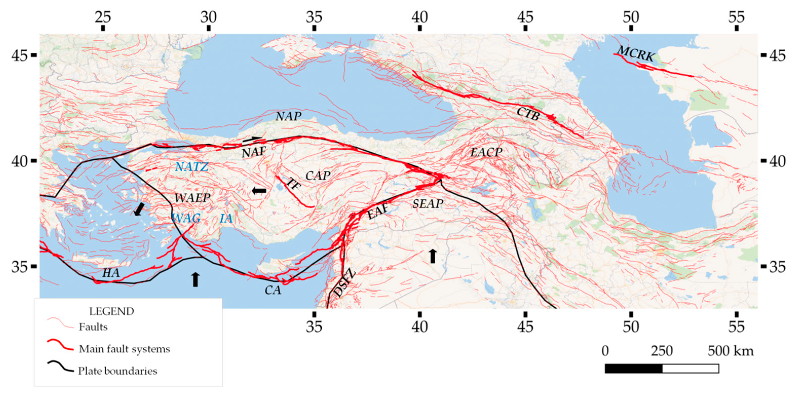
2. Tectonic Setting of the Investigated Area

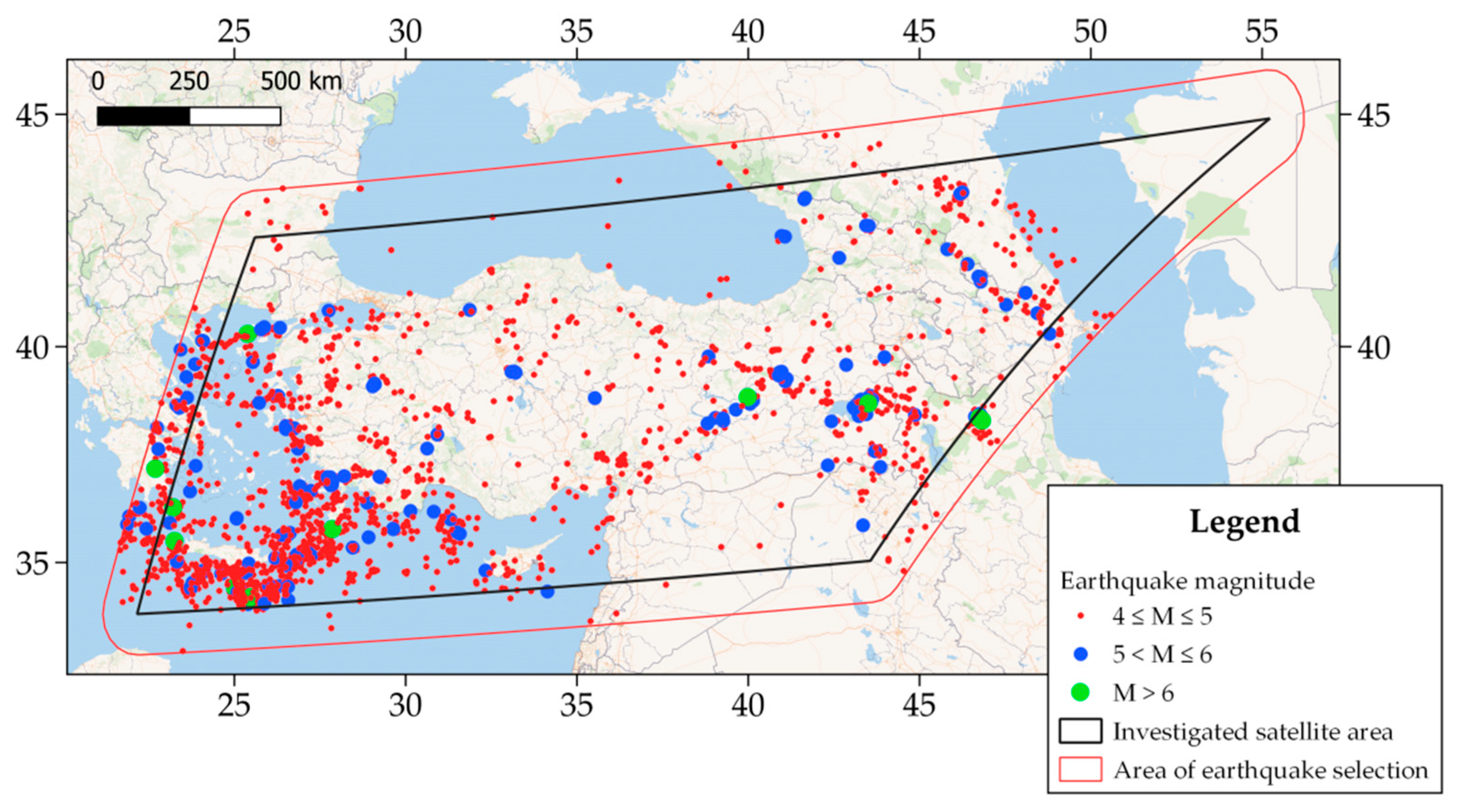
Turkey and neighbouring regions in the eastern Mediterranean Sea are characterised by high seismicity and such rapid deformations that they are considered a natural laboratory, which is helping to better understand the complex processes in collision areas [58]. Turkey is in 10th place within the 50 most seismically active areas in the world [59].

The plate tectonic framework of the region, firstly described in the 1970s (see, for example, [60,61]), is governed by three major tectonic plates—African, Arabian, and Eurasian—together with the Aegean and Anatolian minor plates. The tectonics of the area are strongly influenced by the northward subduction of the African plate below western Turkey and the Aegean region and the collision in the Caucasus and eastern Turkey [58].

Some authors [62], modifying an original scheme [63,64], identify the following five provinces showing different tectonic characteristics: North Anatolian Province (NAP), Eastern Anatolian Contractional Province (EACP), Central Anatolian Province (CAP), Western Anatolian Extensional Province (WAEP), and Southeast Anatolia Province (SEAP). EACP is under an S-N compressional tectonic regime, CAP is characterised by recent complex tectonic activity mainly with strike-slip faults, NAP, with very low microseismicity, is the area between the Black Sea and the North Anatolian Fault (NAF) system, SEAP, characterised by weak seismicity, represents the foreland of the Southeast Anatolian thrust zone, and WAEP is under an N-S extensional faulting mechanism. WAEP is further divided into smaller blocks such as the West Anatolia Graben (WAG) systems, the Isparta Angle (IA), and the Northwest Anatolia Transition Zone (NATZ).

The dextral NAF Zone, the sinistral East Anatolian Fault (EAF) Zone, the Hellenic (HA) and Cyprian Arcs (CA), as well as the sinistral Dead Sea Fault Zone (DSFZ), are the main plate boundaries, i.e., the most important tectonic structures [62,65] of the investigated area. Other relevant tectonic lineaments are the Middle Caspian Region-Kazakhstan fault system, the Eskişehir and Tuzgölü faults, which separate the CAP and WEAP, and the Caucasus thrust belt, representing the northern limit of the EACP.

Figure 1 gives an overview of the above-mentioned tectonic provinces and main fault systems.

3. Data

The following sections give some details about the satellite data and seismic information analysed and used in this paper.

3.1. Satellite Data

The long-term analysis described in this paper is based on a 12-year-long series of night-time (time slot 00:00 GMT) MSG-SEVIRI satellite data. The time series consists of images acquired in the TIR spectral band centred at 10.8 μm (9.8–11.8 μm) from May 2004 to October 2015. From full disk MSG-SEVIRI images, we have cut out and analysed an area centred over Turkey (top-left 42.38 N 25.61 E; top-right 44.88 N 55.13 E; bottom-right 35.06 N 43.55 E; bottom-left 33.78 N 22.18 E, see the black line in Figure 2). In this area, each SEVIRI pixel covers a surface of about 4.5 km (longitude) × 4.7 km (latitude).

A total of 3831 mid-night images represents the analysed data set (Ⴈ), which has been organised on a monthly basis.

3.2. Seismic and Tectonic Information

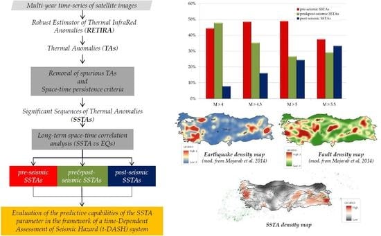
The performed analysis has taken account of seismic events with a magnitude greater than or equal to four (M ≥ 4) recorded in the catalogue of the United States Geological Survey [71]. The catalogue reports 2484 seismic events in the Turkish territory and neighbouring areas from April 2004 to October 2015. The actual area of the earthquake selection is one degree wider than the satellite cut area (see the red line in Figure 2). The distribution of seismic events shows a greater concentration along with the Hellenic Arc, the Isparta Angle, the East, and North Anatolian fault systems.

Since earthquake clusters could affect the results [72], following the approach described in [49] and before the correlation analysis, we filtered the events selecting among those that occurred on the same day within an epicentre-to-epicentre distance of 0.1 degree, the one with the highest magnitude. The resulting “filtered” catalogue, consisting of 2328 events, represents the reference seismic database used in the following analysis.

4. Methodology

4.1. The Robust Estimator of Thermal InfraRed Anomalies (RETIRA)

Details about the methodology used in this paper and its previous applications are summarized in [17,73]. In this section, we want just to recall that the RST approach rests on the Robust Estimator of TIR Anomalies (RETIRA) index, whose more general expression is the following:

$${\otimes }_{\Delta T}\left(\mathit{r},t,L\right)\equiv \frac{\Delta T\left(\mathit{r},t,L\right)-{\mu }_{\Delta T}\left(\mathit{r},L\right)}{{\sigma }_{\Delta T}\left(\mathit{r},L\right)}$$

(1)

where:

• r ≡ (x,y) indicates the geographical coordinates of the satellite pixel centre;
• t is the satellite acquisition time with t ϵ Ⴈ, being Ⴈ the temporal support [31] identifying the time series of homogeneous (same month of the year, same time of the day) collection of images;
• ∆T(r,t) = T(r,t) − T(t) is the difference between the TIR brightness temperature T(r,t) and the spatial average T(t) of T(r,t) on the image at hand. It should be stressed that T(t) computation takes account only of cloud-free pixels, within the investigated region, which are part of the identical category (i.e., only sea or land pixels if r is on the sea or land, respectively);
• μ_∆T(r,L) and σ_∆T(r,L) are, respectively, the temporal mean and standard deviation of ∆T(r,t,L) computed on cloud-free pixels belonging to the chosen dataset (t ϵ Ⴈ). On a monthly basis, we generated two images (μ_∆T and σ_∆T images) used as ‘reference images’ for the calculation of the RETIRA index. They are representative of expected monthly thermal conditions. To reduce the possible negative impact of the massive presence and/or asymmetric spatial distribution of meteorological clouds on the computation of reference fields and the consequent proliferation of possible false positives (reported, for instance, in [26,35,46]), we adopted here the improved RST pre-processing phases firstly proposed by [49];
• L × L represents the dimension (in pixel units) of the elementary spatial unit centred at location r. L = 1 corresponds to the RETIRA classical configuration (used for Turkey already by [25,56]). For L > 1 (only odd numbers), the variable ∆T(r,t,L) is the spatial mean of the punctual cloud-free ∆T(r’,t) values belonging to the L × L pixel box, centred at location r. In all computation phases, the box is considered cloudy when a threshold percentage CT (Cloud Threshold) of cloudy pixels within the L × L pixel box is overcome;
• we define Thermal Anomaly (TA) as a (not-cloudy) location where ⊗_∆T(r,t,L) ≥ K.

The configuration with L > 1 demonstrated (see [11,13] who chose L = 3) to be particularly useful in reducing sporadic and spatially localized TIR anomalies (e.g., due to forest fires, gas-flaring, or accidents related to industrial activities), saving or even highlighting, at the same time, spatially extended TIR anomalous transients, as expected (see next section) in the case of fluctuations related to seismic events. In this paper, K = 3 and, similarly in [11,13], L = 3 and CT = 55% were chosen. The OCA (One-channel Cloudy-radiance-detection Approach, [74]) algorithm was used everywhere to identify cloudy pixels.

4.2. Space-Time Persistence Criteria, Significant Thermal Anomalies (STAs) and Significant Sequences of Thermal Anomalies(SSTAs) Definitions

As explained in detail in previous papers [25,26,35,46], natural and observational particular conditions may generate spurious TAs, which have recognisable features (e.g., cloud shadows, coastline shape replication), often appearing isolated in the space (i.e., punctual) and time (i.e., sporadic) domain. Unlike them, the TAs possibly associated with earthquakes are expected (see [17,73] and references therein) to be persistent in the space (e.g., affected area) and time domains (e.g., at least N repetitions within D days). To this aim, specific selection criteria on TAs have been introduced to discard spurious TAs, saving the ones possibly associated with seismic activity and, for this reason, named Significant Thermal Anomalies (STAs). In this paper, in order to isolate STAs, the same criteria adopted in [11,13,49,54] were applied. This can be so summarised in the following:

• Identification and removal of spurious TAs due to massive (more than 80% of pixels) presence of clouds on the scene and/or to the so-called ‘cold spatial average effect’ [26,46]. In both cases, land and sea pixels are separately considered (so that a land/sea TA is excluded if more than 80% of land/sea pixels in the scene are, respectively, cloudy). Similarly, a land/sea TA is removed if the following expression T(t’) > μ_T—2σ_T is verified, being T(t’) the spatial average of T(r,t) computed on the cloud-free, land/sea pixels of the image at hand (acquired at time t = t’), μ_T and σ_T are, respectively, the temporal average and standard deviation of T(t), computed using the homogeneous dataset of images belonging to the temporal domain Ⴈ.
  • Navigation and co-location errors. TAs close to coastlines clearly replicating their shape [35] are easily identified and removed;
  • Other known spurious effects. TAs associated with the effects reported in [26,46,49,54] are easily identified and removed.

Moreover, a single STA is considered part of a Significant Sequence of Thermal Anomalies (SSTA) if:

• Spatial persistence: it is not spatially isolated being part of a group of STAs (1-degree maximum away from each other) covering an area (affected area) ≥150 km²;
• Temporal persistence: the same STAs reappears at least another time in the seven preceding/following days.

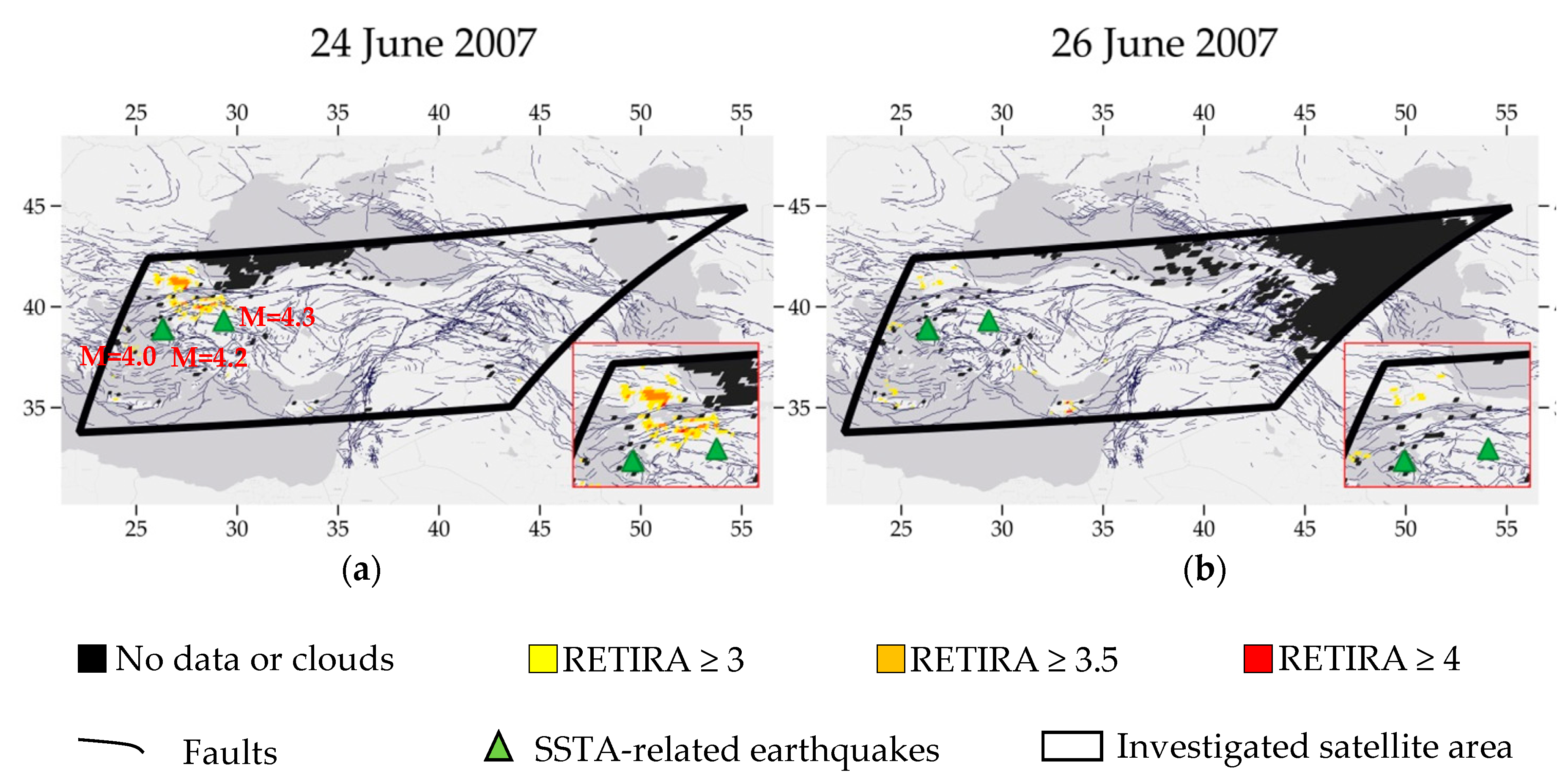
5. Data Analysis and Results

Applying the aforementioned rules to all SEVIRI TIR images from May 2004 to October 2015, we identified 155 SSTAs in the whole time series.

We performed a correlation analysis between SSTA appearances and the location, time, and magnitude in the seismic events of the filtered catalogue. To this aim, we applied empirical rules based on previous studies (see [17,73] and references therein) and physical models (e.g., [20]) proposed to explain TA appearances before and after large earthquakes. In detail, we considered each STA observed at a geographical site (x,y) at the time t and belonging to a specific SSTA, in correlation with an M ≥ 4 seismic event, if the earthquake takes place within the following space-time correlation volume:

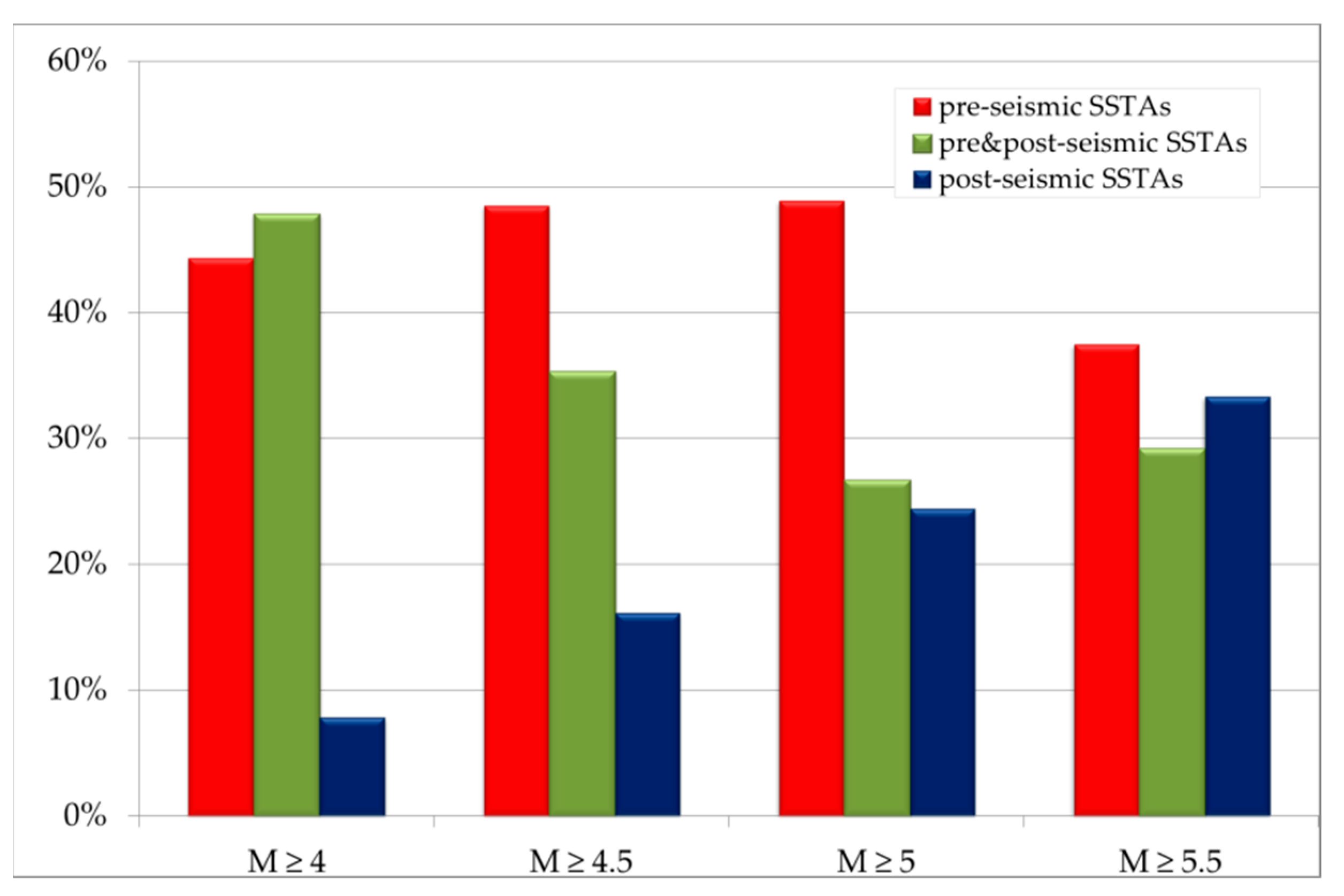
• Temporal window: up to 30 days after (pre-earthquake anomaly) the last or until 15 days before (postseismic/coseismic anomaly) the first appearance of TAs;
• Spatial window: within a distance D ≤ R from whatever TAs belonging to the considered SSTA. The distance D is defined under the conditions of 150 km ≤ R ≤ 10^0.43M, the upper limit being the Dobrovolsky radius (in km) [75], corresponding to an earthquake of magnitude M.

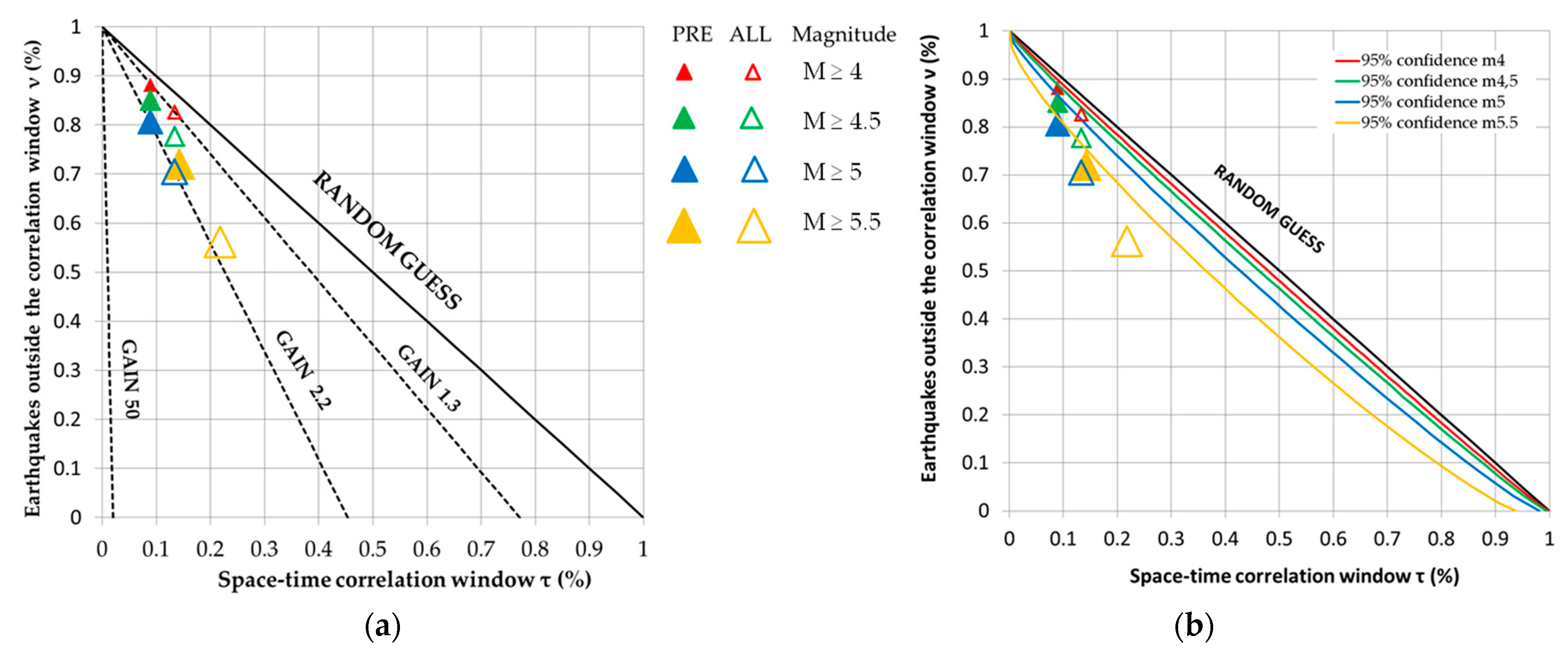
The space-time correlation analysis based on the above-mentioned rules highlights that 115 SSTAs (74%) out of 155 could be related to seismic events, while the remaining 40 SSTAs (26%) turn out to be false positives. An example of an earthquake-related SSTA is in Figure 3.

More detailed analysis of the earthquake-correlated SSTAs showed that 51 out of 115 (44%) precede the related seismic event, 9 out of 115 (8%) just follow the correlated earthquake (post-seismic SSTAs), and the remaining 55 (48%) appear between two or more earthquakes (pre & post-seismic SSTAs).

In addition, we also analysed the earthquake correlated SSTAs versus the magnitude of related events (Figure 4). It is worth noting that pre-seismic SSTAs always prevail over post-seismic ones, with a decreasing difference as far as the magnitude limit increases.

It should be noted that, from an OEF (Operational Earthquake Forecast) point of view, the pre & post-seismic SSTAs are of scarce importance. In fact, their appearance between the times of occurrence of different earthquakes cannot be interpreted in relation to future seismic events, but rather to already occurred events. As the goal of this work is still not to provide an OEF, in order to try to solve such an ambiguity, each pre & post-seismic SSTA has been re-classified as pre-seismic (post-seismic) if it occurs before (after) the time of occurrence of the earthquake, with the higher magnitude among the ones included in its space-time correlation volume. In case more than one seismic event shares the same magnitude, the closest event in the space domain has been retained. After this re-classification, the number of pre-seismic SSTAs passes from 51 (48%) to 72 (63%), and post-seismic SSTAs passes from 9 (8%) to 43 (37%). Figure 5, reporting the results of such an analysis with reference to earthquake magnitudes, confirms the prevailing appearance of the SSTAs before earthquakes. In particular, although differences poorly change with the magnitudes, the trend of pre-seismic SSTAs seems to increase slightly with the magnitude. However, such a prevalence could be simply due to the fact that the considered pre-seismic temporal window is double the duration (30 days) of the post-seismic one (15 days). So that, after normalizing such a result from this effect, just a small prevailing of post-seismic SSTAs can be registered (from 6% up to 0% moving from the lowest to the highest magnitude class) in comparison with pre-seismic ones.

To better evaluate the significance of the achieved results, the Molchan error diagram ([76] and references therein) was considered. In particular, a customised version of such an approach, fully described in previous papers [11,49], allows us to verify the actual value of the SSTAs as compared with a random alarm function. It plots ν(M), i.e., the percentage of the earthquakes with a magnitude greater than (or equal to) M that are not preceded or followed by SSTAs (i.e., missed earthquakes), versus τ(M), i.e., the percentage of the warned space-time volume considering earthquakes with a magnitude greater than (or equal to) M. These two parameters, ν(M) and τ(M), are computed according to the following equations:

$$\nu \left(\mathrm{M}\right)=\frac{Number of EQs with magnitude \ge M outside the correlation volume \left(missed\right) }{Total number of EQs with magnitude \ge M occurred within the whole investigated space\times time volume}$$

(2)

$$\tau \left(\mathrm{M}\right)=\frac{Total alerted space\times time volume for EQs with magnitude \ge M}{Whole investigated space\times time volume}$$

(3)

In addition, following Aki [77], the probability gain lines were calculated as ν = 1—Gτ (where G represents the probability gain) together with the confidence limit curves, based on the null-hypothesis (see [78]), at levels of 95% surrounding the diagonal of a random guess.

Figure 6 shows the result of the error diagram. The events are analysed by magnitude classes, referring to all earthquake-related SSTAs (‘ALL’) or just to the pre-seismic (‘PRE’) ones. In both cases, the data fall within the optimal strategy zone (left side) with a “significant” deviation from random guessing (i.e., confidence levels of 95%) and, therefore, a non-casual correlation between the SSTAs and earthquakes may be assumed. Looking at the probability gain (Figure 6a), we find values between 1.3 (for M ≥ 4) and 2.2 (for M ≥ 5).

It should be noted that:

(a)

The non-casual correlation, found in the ‘ALL’ case, confirms those models (e.g., [20]), suggesting the possible appearance of thermal anomalies both before and/or after seismic events;

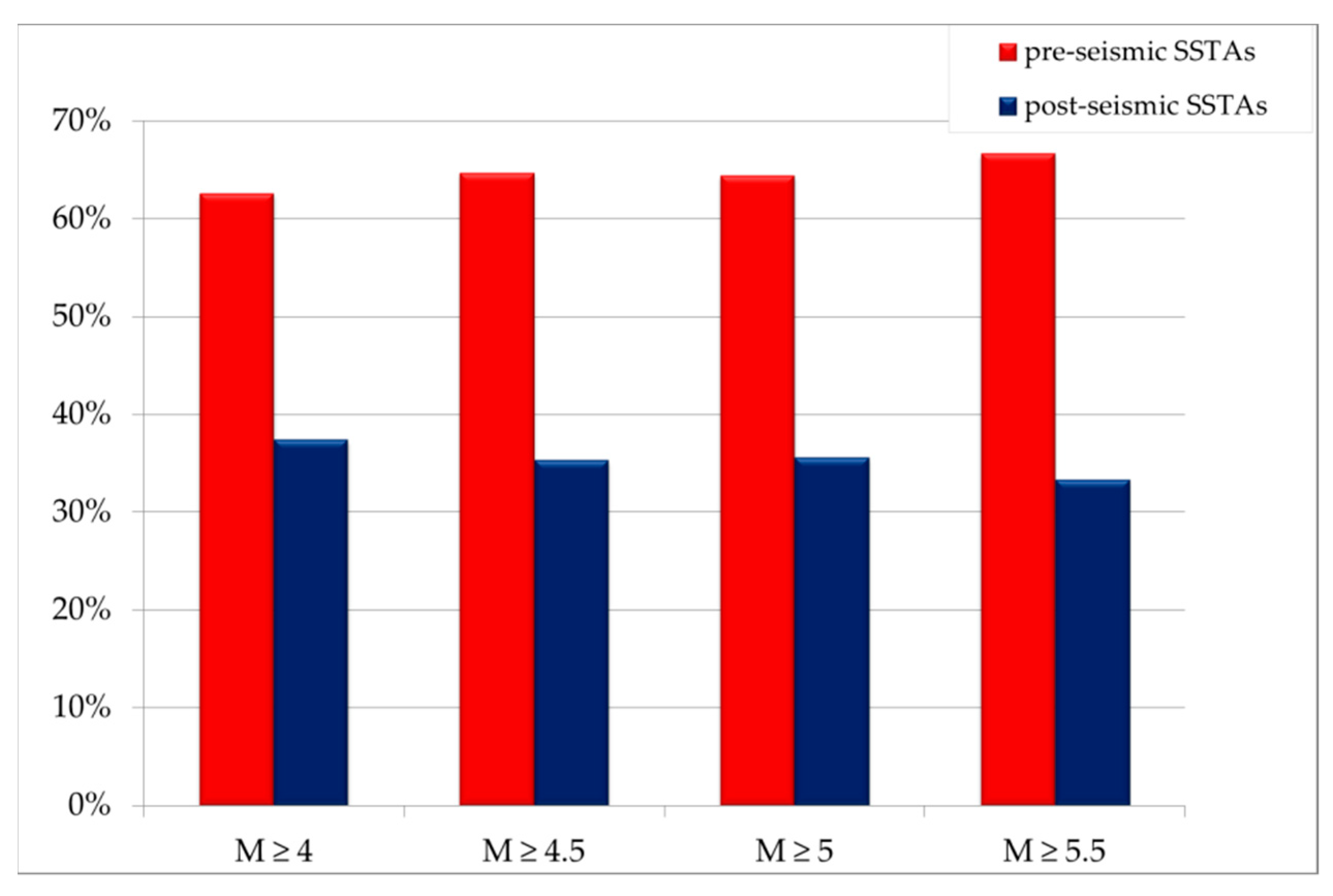
(b)

The non-casual correlation, found in the ‘PRE’ case, confirms, instead, the predictive capability of the considered parameter;

(c)

The gain factor seems to be greater for higher (and rarer) magnitude class events, reinforcing the idea that the correlation is driven by physical relations and not just by the high number of events.

Such results, which are in line with the ones achieved by the previous, already quoted, similar studies, also confirm a regional dependence that can be recognized by looking, for instance, at the achieved false-positive rates. Applying similar RST analyses to comparably long (≥10 years) time series over Greece [49], Italy [13], and Japan [11], report quite different false-positive rates (respectively 7%, 40%, 38% to be compared with the 26% of this study) depending on the considered region. The false-positive rate, better than other indicators, can qualify the predictive capabilities of the considered parameter (i.e., thermal anomalies based on RST analyses) within a multi-parametric t-DASH system, even if just in terms of the reliability of the forecast. In fact, the missing rate, another important indicator, would be strongly underestimated in this case due to the possible presence of meteorological clouds, preventing TIR radiation from reaching the satellite sensor.

Quite extended space/time data gaps can be responsible for a number of “missed” events just due to the absence of the satellite measurements that are useful to identify possible SSTAs. To give an idea, 65% of TIR observations used by [11] over Japan were discarded due to the massive presence of clouds; 26% of images were discarded for the same reason in this study.

Such variability of results, already reported by [11] for different regions of Japan (apparently in association with the latitudinal variation of the local meteorological regimes), has been investigated for Turkey (for regions that are mostly at the same latitudes) in relation to seismogenic fault distribution.

To this aim, an analysis concerning the SSTA spatial distribution was carried out in order to highlight SSTAs possible concentration in specific areas. As confirmation of the existing link between SSTA appearance and migration of optically active gases, such as CO₂ and CH₄, alongside seismogenic faults (e.g., [23,79]), almost all (more than 99%) SSTAs were found near fault lines or tectonic plate boundaries, but not in all of them. This could be explained by considering the different seismic and/or degassing activity associated with the different fault lines. Figure 7 shows the SSTAs and corresponding fault systems where they are located. SSTAs over the different fault systems (coloured slices of the inner pie chart) are divided into earthquake-related SSTAs (blue slices of the outer pie chart) and earthquake-not-related (red slices of the outer pie chart) are presented. It is worth noting that:

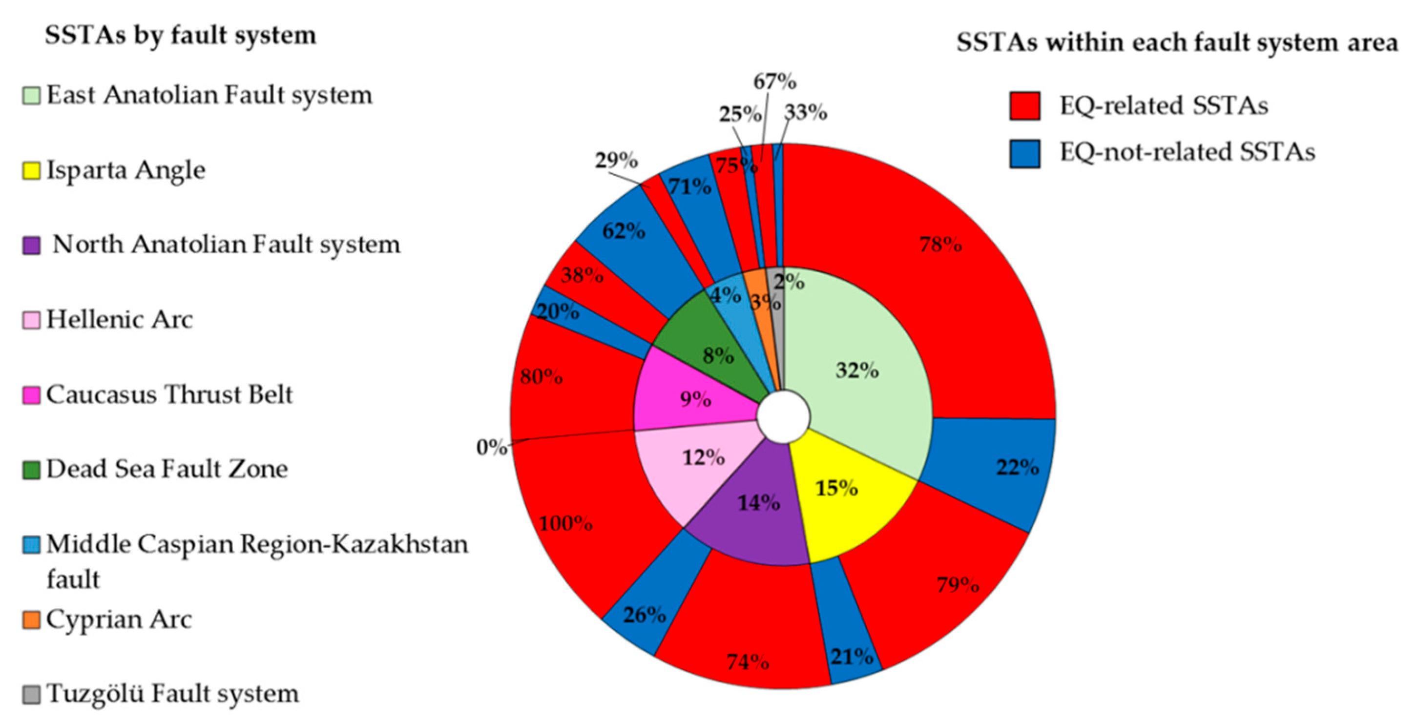
• The greatest number of SSTAs are located along with the East Anatolian Fault system (32%), with about 80% of earthquake-related ones (i.e., 20% of false positives);
• The Isparta Angle and the North Anatolian Fault system register 15% and 14% of the total identified SSTAs, respectively; 80% of successes (i.e., 20% of false positives) are associated with the former, about 75% of successes (i.e., 25% of false positives) with the latter;
• SSTAs in the correspondence of the Hellenic Arc represent about 10% of all identified sequences. All such SSTAs are related to seismic events (100% of success, zero false positives);
• 9% of SSTAs are in correspondence with the Caucasus Thrust Belt, where 80% are earthquake-related (i.e., 20% of false positives), and 8% of SSTAs are along the Dead Sea Fault Zone (about 40% of the success rate);
• A small number of SSTAs are located over the Middle Caspian Region-Kazakhstan fault (4%), the Cyprian Arc (3%), and the Tuzgölü Fault region (2%). The success rate is about 30%, 75%, and 65%, respectively.

Just focusing on the Turkish territory, results on NAF, EAF, IA, and TF were compared with the earthquake and fault densities by [80] (Figure 8), also in agreement with Figure 1 and Figure 2. It is worth noting that the region of the Tuzgölü Fault has a medium-low value of fault density but a very low density of seismic activity. That is in line with the very low percentage of identified SSTAs along with this fault system (2%, corresponding to 3 SSTAs, one of them is earthquake-correlated). On the whole, there is a good correspondence between the areas with a greater number of identified SSTAs (NAF, EAF, IA) and higher values of earthquake density. Such a comparison suggests that SSTAs are not simply related to fault systems (indeed, they appear quite often there), but particularly to those that are seismically active.

6. Conclusions

In this paper, a long-term correlation analysis was performed for the first time over Turkey and neighbouring areas in order to fully characterise the predictive capabilities of the parameter TIR anomaly identified by an RST-RETIRA analysis to be a “candidate” in the framework of a time-Dependent Assessment of Seismic Hazard (t-DASH) system [13,73].

To this aim, a 12-year-long series (about 4000 images) of SEVIRI-MSG images collected in the period of April 2004–October 2015 was analysed using the RST methodology to first identify the TIR anomalies and then SSTAs. A correlation analysis was carried out in order to evaluate the possible correlation of a SSTA appearance with earthquakes (with M ≥ 4) that occurred within a predefined space-time volume in the investigated region/period. In order to evaluate a possible dependence on sub-regional seismic aspects (namely fault density and seismic activity), the analysis was also performed for the sub-regions corresponding to different fault systems.

The analysis allowed us to identify 155 SSTAs on the whole for the period and the whole area of interest. Of which, 74% of them appear earthquake-related (i.e., the false-positive rate is 26%), occurring within the pre-defined space–time correlation volume around the time and location of the occurrence of M ≥ 4 earthquakes. The random error test performed using a customised Molchan diagram proved that the appearance of SSTAs in spatial/temporal correspondence with seismic events was not casual. Compared with the random guess, we found probability gain values from 1.3 to 2.2 (for M ≥ 4 and M ≥ 5 earthquakes, respectively).

Finally, an additional analysis was carried out considering the SSTA distribution over the main fault systems that affect the Anatolian Provinces and neighbouring areas. It is noticeable that SSTAs seem to appear much more where the seismic density is higher than where the fault density is higher (for instance, along with the East Anatolian Fault system and not in the Tuzgölü Fault area, Figure 8), confirming the dynamic relationship of SSTAs with actual seismicity more than with static tectonic settings. The fact that results are different in the different considered regions (such as in the Hellenic Arc where the false-positive rate reaches the zero value on 19 identified SSTAs) confirms their dependence on specific local/regional tectonic, seismic, and probably also geochemical settings, as shown by the variety of results achieved in previous similar studies [11,13,49,54].

References

1. Bormann, P. From Earthquake Prediction Research to Time-Variable Seismic Hazard Assessment. Applications. Pure Appl. Geophys. 2011, 168, 329–366. [Google Scholar] [CrossRef]
2. Vanneste, K.; Stein, S.; Camelbeeck, T.; Vleminckx, B. Insights into earthquake hazard map performance from shaking history simulations. Sci. Rep. 2018, 8, 1855. [Google Scholar] [CrossRef] [PubMed] [Green Version]
3. Albarello, D. State of the art on short-term earthquake forecasting and preparation in Italy: A preface. Boll. Geofis. Teor. Appl. 2015, 56, 71–82. [Google Scholar] [CrossRef]
4. Isikara, A.M.; Vogel, A. A Multidisciplinary Approach to Earthquake Prediction. Review of the Interdisciplinary Conference on Earthquake Prediction Research in the North Anatolian Fault Zone. Dev. Solid Earth Geophys. 1983, 15, 41. [Google Scholar] [CrossRef]
5. Eftaxias, K. Footprints of non-extensive Tsallis statistics, self-affinity and universality in the preparation of the L’Aquila earthquake hidden in a pre-seismic EM emission. Phys. A Stat. Mech. Appl. 2010, 389, 133–140. [Google Scholar] [CrossRef]
6. Ouzounov, D.; Pulinets, S.; Hattori, K.; Taylor, P. Pre-Earthquake Processes: A Multidisciplinary Approach to Earthquake Prediction Studies; Geophysical Monograph Series; John Wiley & Sons Inc.: Hoboken, NJ, USA, 2018; 365p. [Google Scholar]
7. Yuce, G.; Ugurluoglu, D.Y.; Adar, N.; Yalcin, T.; Yaltirak, C.; Streil, T.; Oeser, V. Monitoring of earthquake precursors by multi-parameter stations in Eskisehir region (Turkey). Appl. Geochem. 2010, 25, 572–579. [Google Scholar] [CrossRef]
8. Jing, F.; Shen, X.H.; Kang, C.L.; Xiong, P. Variations of multi-parameter observations in atmosphere related to earthquake. Nat. Hazards Earth Syst. Sci. 2013, 13, 27–33. [Google Scholar] [CrossRef] [Green Version]
9. Venkatanathan, N.; Yang, Y.C.; Lyu, J. Observation of abnormal thermal and infrasound signals prior to the earthquakes: A study on Bonin Island earthquake M7.8 (May 30, 2015). Environ. Earth Sci. 2017, 76, 228. [Google Scholar] [CrossRef]
10. Chetia, T.; Sharma, G.; Dey, C.; Raju, P.L.N. Multi-Parametric Approach for Earthquake Precursor Detection in Assam Valley (Eastern Himalaya, India) using Satellite and Ground Observation Data. Geotectonics 2020, 54, 83–96. [Google Scholar] [CrossRef]
11. Genzano, N.; Filizzola, C.; Hattori, K.; Pergola, N.; Tramutoli, V. Statistical correlation analysis between thermal infrared anomalies observed from MTSATs and large earthquakes occurred in Japan (2005–2015). J. Geophys. Res. Solid Earth 2021, 126, e2020JB020108. [Google Scholar] [CrossRef]
12. Shebalin, P.N.; Narteau, C.; Zechar, J.; Holschneider, M. Combining earthquake forecasts using differential probability gains. Earth Planets Space 2014, 66, 37. [Google Scholar] [CrossRef] [Green Version]
13. Genzano, N.; Filizzola, C.; Lisi, M.; Pergola, N.; Tramutoli, V. Toward the development of a multi parametric system for a short-term assessment of the seismic hazard in Italy. Ann. Geophys 2020, 63, PA550. [Google Scholar] [CrossRef]
14. Wyss, M. Evaluation of Proposed Earthquake Precursors; AGU: Washington, DC, USA, 1991; Volume 32. [Google Scholar]
15. Ingebritsen, S.; Manga, M. Hydrogeochemical precursors. Nat. Geosci. 2014, 7, 697–698. [Google Scholar] [CrossRef]
16. Woith, H. Radon earthquake precursor: A short review. Eur. Phys. J. Spec. Top. 2015, 224, 611–627. [Google Scholar] [CrossRef]
17. Tramutoli, V.; Corrado, R.; Filizzola, C.; Genzano, N.; Lisi, M.; Pergola, N. From visual comparison to Robust Satellite Techniques: 30 years of thermal infrared satellite data analyses for the study of earthquake preparation phases. Boll. Geofis. Teor. Appl. 2015, 56, 167–202. [Google Scholar] [CrossRef]
18. Tronin, A.A. Satellite thermal survey—A new tool for the study of seismoactive regions. Int. J. Remote Sens. 1996, 17, 1439–1455. [Google Scholar] [CrossRef]
19. Qiang, Z.; Xu, X.; Dian, C. Case 27 thermal infrared anomaly precursor of impending earthquakes. Pure Appl. Geophys. 1997, 149, 159–171. [Google Scholar] [CrossRef]
20. Tramutoli, V.; Aliano, C.; Corrado, R.; Filizzola, C.; Genzano, N.; Lisi, M.; Martinelli, G.; Pergola, N. On the possible origin of thermal infrared radiation (TIR) anomalies in earthquake-prone areas observed using robust satellite techniques (RST). Chem. Geol. 2013, 339, 157–168. [Google Scholar] [CrossRef]
21. Freund, F.T. Pre-earthquake signals—Part I: Deviatoric stresses turn rocks into a source of electric currents. Nat. Hazards Earth Syst. Sci. 2007, 7, 535–541. [Google Scholar] [CrossRef] [Green Version]
22. Pulinets, S.A.; Ouzounov, D. Lithosphere–Atmosphere–Ionosphere Coupling (LAIC) model—An unified concept for earthquake precursors validation. J. Asian Earth Sci. 2011, 41, 371–382. [Google Scholar] [CrossRef]
23. Irwin, W.P.; Barnes, I. Tectonic relations of carbon dioxide discharges and earthquakes. J. Geophys. Res. 1980, 85, 3115–3121. [Google Scholar] [CrossRef]
24. Scholz, C.H.; Sykes, L.R.; Aggarwal, Y.P. Earthquake prediction: A physical basis. Science 1973, 181, 803–810. [Google Scholar] [CrossRef] [PubMed]
25. Tramutoli, V.; Cuomo, V.; Filizzola, C.; Pergola, N.; Pietrapertosa, C. Assessing the potential of thermal infrared satellite surveys for monitoring seismically active areas: The case of Kocaeli (İzmit) earthquake, August 17, 1999. Remote Sens. Environ. 2005, 96, 409–426. [Google Scholar] [CrossRef]
26. Genzano, N.; Aliano, C.; Corrado, R.; Filizzola, C.; Lisi, M.; Mazzeo, G.; Paciello, R.; Pergola, N.; Tramutoli, V. RST analysis of MSG-SEVIRI TIR radiances at the time of the Abruzzo 6 April 2009 earthquake. Nat. Hazards Earth Syst. Sci. 2009, 9, 2073–2084. [Google Scholar] [CrossRef]
27. Lisi, M.; Filizzola, C.; Genzano, N.; Grimaldi, C.S.L.; Lacava, T.; Marchese, F.; Mazzeo, G.; Pergola, N.; Tramutoli, V. A study on the Abruzzo 6 April 2009 earthquake by applying the RST approach to 15 years of AVHRR TIR observations. Nat. Hazards Earth Syst. Sci. 2010, 10, 395–406. [Google Scholar] [CrossRef]
28. Pergola, N.; Aliano, C.; Coviello, I.; Filizzola, C.; Genzano, N.; Lacava, T.; Lisi, M.; Mazzeo, G.; Tramutoli, V. Using RST approach and EOS-MODIS radiances for monitoring seismically active regions: A study on the 6 April 2009 Abruzzo earthquake. Nat. Hazards Earth Syst. Sci. 2010, 10, 239–249. [Google Scholar] [CrossRef]
29. Barka, A. The 17th August 1999 Izmit Earthquake. Science 1999, 285, 1858–1859. [Google Scholar] [CrossRef]
30. Lucente, F.P.; Gori, P.D.; Margheriti, L.; Piccinini, D.; Bona, M.D.; Chiarabba, C.; Agostinetti, N.P. Temporal variation of seismic velocity and anisotropy before the 2009 MW 6.3 L’Aquila earthquake, Italy. Geology 2010, 38, 1015–1018. [Google Scholar] [CrossRef]
31. Tramutoli, V. Robust AVHRR Techniques (RAT) for Environmental Monitoring: Theory and Applications; Zilioli, E., Ed.; Society of Photo Optical: Bellingham, WA, USA, 1998; Volume 3496, pp. 101–113. [Google Scholar] [CrossRef]
32. Tramutoli, V. Robust satellite techniques (RST) for natural and environmental hazards monitoring and mitigation: Theory and applications. In Proceedings of the International Workshop on the Analysis of Multi-temporal Remote Sensing Images, Leuven, Belgium, 18–20 July 2007. [Google Scholar] [CrossRef]
33. Tramutoli, V.; Di Bello, G.; Pergola, N.; Piscitelli, S. Robust satellite techniques for remote sensing of seismically active areas. Ann. Geofis. 2001, 44, 295–312. [Google Scholar] [CrossRef]
34. Di Bello, G.; Filizzola, C.; Lacava, T.; Marchese, F.; Pergola, N.; Pietrapertosa, C.; Piscitelli, S.; Scaffidi, I.; Valerio, T. Robust satellite techniques for volcanic and seismic hazards monitoring. Ann. Geophys. 2004, 47, 49–64. [Google Scholar] [CrossRef]
35. Filizzola, C.; Pergola, N.; Pietrapertosa, C.; Tramutoli, V. Robust satellite techniques for seismically active areas monitoring: A sensitivity analysis on September 7, 1999 Athens’s earthquake. Phys. Chem. Earth 2004, 29, 517–527. [Google Scholar] [CrossRef]
36. Eneva, M.D.; Adams, N.; Wechsler, Y.; Ben-Zion, Y.; Dor, O. Thermal Properties of Faults in Southern California from Remote Sensing Data; Report Sponsored by NASA under Contract to SAIC No. NNH05CC13C; NASA Goddard Space Flight Center: Greenbelt, MD, USA, 2008; p. 70. [Google Scholar]
37. Halle, W.; Oertel, D.; Schlotzhauer, G.; Zhukov, B. Early Warning of Earthquakes by Space-Borne Infrared Sensors [Erdbebenfrüherkennung mit InfraRot Sensoren aus dem Weltraum]; Institut für Robotik und Mechatronik Optische Informationssysteme: Berlin, Germany, 2008; pp. 1–106. [Google Scholar]
38. Li, J.; Wu, L.; Dong, Y.; Liu, S.; Yang, X. An quantitative model for tectonic activity analysis and earthquake magnitude predication based on thermal infrared anomaly. In Proceedings of the IEEE International Symposium on Geoscience and Remote Sensing (IGARSS), Barcelona, Spain, 23–28 July 2007; pp. 3039–3042. [Google Scholar] [CrossRef]
39. Akhoondzadeh, M. A comparison of classical and intelligent methods to detect potential thermal anomalies before the 11 August 2012 Varzeghan, Iran, earthquake (Mw = 6.4). Nat. Hazards Earth Syst. Sci. 2013, 13, 1077–1083. [Google Scholar] [CrossRef]
40. Xiong, P.; Gu, X.F.; Bi, Y.X.; Shen, X.H.; Meng, Q.Y.; Zhao, L.M.; Kang, C.L.; Chen, L.Z.; Jing, F.; Yao, N.; et al. Detecting seismic IR anomalies in bi-angular Advanced Along-Track Scanning Radiometer data. Nat. Hazards Earth Syst. Sci. 2013, 13, 2065–2074. [Google Scholar] [CrossRef] [Green Version]
41. Xiong, P.; Shen, X.; Gu, X.; Meng, Q.; Zhao, L.; Zhao, Y.; Li, Y.; Dong, J. Seismic infrared anomalies detection in the case of the Wenchuan earthquake using bi-angular advanced along-track scanning radiometer data. Ann. Geophys. 2015, 58, S0217. [Google Scholar] [CrossRef]
42. Bellaoui, M.; Hassini, A.; Bouchouicha, K. Pre-seismic anomalies in remotely sensed land surface temperature measurements: The case study of 2003 Boumerdes earthquake. Adv. Space Res. 2017, 59, 2645–2657. [Google Scholar] [CrossRef]
43. Khalili, M.; Panah, S.K.A.; Eskandar, S.S.A. Using Robust Satellite Technique (RST) to determine thermal anomalies before a strong earthquake: A case study of the Saravan earthquake (April 16th, 2013, MW = 7.8, Iran). J. Asian Earth Sci. 2019, 173, 70–78. [Google Scholar] [CrossRef]
44. Kouli, M.; Peleli, S.; Saltas, V.; Makris, J.; Vallianatos, F. Robust Satellite Techniques for mapping thermal anomalies possibly related to seismic activity of March 2021, Thessaly Earthquakes. BGSG 2021, 58, 105–130. [Google Scholar] [CrossRef]
45. Mukhopadhyay, U.K.; Sharma, R.N.K.; Anwar, S.; Dutta, A.D. Earthquakes and Thermal Anomalies in a Remote Sensing Perspective. In Machine Learning and Big Data Analytics Paradigms: Analysis, Applications and Challenges. Studies in Big Data; Hassanien, A.E., Darwish, A., Eds.; Springer: Cham, Switzerland, 2021; Volume 77. [Google Scholar] [CrossRef]
46. Aliano, C.; Corrado, R.; Filizzola, C.; Genzano, N.; Pergola, N.; Tramutoli, V. TIR Satellite Techniques for monitoring Earthquake active regions: Limits, main achievements and perspectives. Ann. Geophys. 2008, 51, 303–317. [Google Scholar] [CrossRef]
47. Aliano, C.; Corrado, R.; Filizzola, C.; Pergola, N.; Tramutoli, V. Robust Satellite Techniques (RST) for Seismically Active Areas Monitoring: The Case of 21st May, 2003 Boumerdes/Thenia (Algeria) Earthquake. In Proceedings of the 2007 International Workshop on the Analysis of Multi-temporal Remote Sensing Images, Leuven, Belgium, 18–20 July 2007. [Google Scholar] [CrossRef] [Green Version]
48. Genzano, N.; Aliano, C.; Filizzola, C.; Pergola, N.; Tramutoli, V. A robust satellite technique for monitoring seismically active areas: The case of Bhuj-Gujarat earthquake. Tectonophysics 2007, 431, 197–210. [Google Scholar] [CrossRef]
49. Eleftheriou, A.; Filizzola, C.; Genzano, N.; Lacava, T.; Lisi, M.; Paciello, R.; Pergola, N.; Vallianatos, F.; Tramutoli, V. Long-Term RST Analysis of Anomalous TIR Sequences in Relation with earthquakes occurred in Greece in the Period 2004–2013. Pure Appl. Geophys. 2016, 173, 285–303. [Google Scholar] [CrossRef] [Green Version]
50. Aliano, C.; Corrado, R.; Filizzola, C.; Genzano, N.; Pergola, N.; Tramutoli, V. Robust satellite techniques (RST) for the thermal monitoring of earthquake prone areas: The case of Umbria-Marche October, 1997 seismic events. Ann. Geophys. 2008, 51, 451–459. [Google Scholar] [CrossRef]
51. Pergola, N.; D’angelo, G.; Lisi, M.; Marchese, F.; Mazzeo, G.; Tramutoli, V. Time domain analysis of Robust Satellite Techniques (RST) for near real-time monitoring of active volcanoes and thermal precursor identification. Phys. Chem. Earth 2009, 34, 380–385. [Google Scholar] [CrossRef]
52. Bonfanti, P.; Genzano, N.; Heinicke, J.; Italiano, F.; Martinelli, G.; Pergola, N.; Telesca, L.; Tramutoli, V. Evidences of CO2-gas emission variations in Central Apennines (Italy) during the L’Aquila seismic sequence (March–April 2009). Boll. Geof. Teor. Appl. 2012, 53, 147–168. [Google Scholar] [CrossRef]
53. Tramutoli, V.; Corrado, R.; Filizzola, C.; Genzano, N.; Lisi, M.; Paciello, R.; Pergola, N. One year of RST based satellite thermal monitoring over two Italian seismic areas. Boll. Geofis. Teor. Appl. 2015, 56, 275–294. [Google Scholar] [CrossRef]
54. Genzano, N.; Filizzola, C.; Paciello, R.; Pergola, N.; Tramutoli, V. Robust Satellite Techniques (RST) for monitoring earthquake prone areas by satellite TIR observations: The case of 1999 Chi-Chi earthquake (Taiwan). J. Asian Earth Sci. 2015, 114, 289–298. [Google Scholar] [CrossRef]
55. Zhang, Y.; Meng, Q. A statistical analysis of TIR anomalies extracted by RSTs in relation to an earthquake in the Sichuan area using MODIS LST data. Nat. Hazards Earth Syst. Sci. 2019, 19, 535–549. [Google Scholar] [CrossRef] [Green Version]
56. Corrado, R.; Caputo, R.; Filizzola, C.; Pergola, N.; Pietrapertosa, C.; Tramutoli, V. Seismically active area monitoring by robust TIR satellite techniques: A sensitivity analysis on low magnitude earthquakes in Greece and Turkey. Nat. Hazards Earth Syst. Sci. 2005, 5, 101–108. [Google Scholar] [CrossRef]
57. Tramutoli, V.; Jakowski, N.; Pulinets, S.; Romanov, A.; Filizzola, C.; Shagimuratov, I.; Pergola, N.; Ouzounov, D.; Papadopulos, G.; Genzano, N.; et al. From PRE-EARTQUAKES to EQUOS: How to exploit multi-parametric observations within a novel system for Time-Dependent Assessment of Seismic Hazard (T-DASH) in a pre-operational Civil Protection context. In Proceedings of the Second European Conference on Earthquake Engineering and Seismology (2ECEES), Instanbul, Turkey, 24–29 August 2014; Abstract Number 3141. Available online: http://www.eaee.org/Media/Default/2ECCES/2ecces_esc/3141.pdf (accessed on 1 November 2021).
58. Taymaz, T.; Yilmaz, Y.; Dilek, Y. The geodynamics of the Aegean and Anatolia: Introduction. Geol. Soc. Spec. Publ. 2007, 291, 1–16. [Google Scholar] [CrossRef]
59. Tsapanos, T.M.; Burton, P.W. Seismic hazard evaluation for specific seismic regions of the world. Tectonophysics 1991, 194, 153–169. [Google Scholar] [CrossRef]
60. McKenzie, D. Active Tectonics of the Mediterranean Region. Geophys. J. Int 1972, 30, 109–185. [Google Scholar] [CrossRef] [Green Version]
61. Dewey, J.F.; Pitman, W.C.; Ryan, W.B.F.; Bonnin, J. Plate tectonics and the evolution of the Alpine System. Geol. Soc. Am. Bull. 1973, 84, 3137–3180. [Google Scholar] [CrossRef]
62. Emre, Ö.; Duman, T.Y.; Özalp, S.; Şaroğlu, F.; Olgun, Ş.; Elmacı, H.; Çan, T. Active fault database of Turkey. Bull. Earthquake Eng. 2018, 16, 3229–3275. [Google Scholar] [CrossRef]
63. Şengör, A.M.C. Mid-Mesozoic closure of Permo-Triassic Tethys and its implications. Nature 1979, 279, 590–593. [Google Scholar] [CrossRef]
64. Şengör, A.M.C. The North Anatolian transform fault: Its age, offset and tectonic significance. J. Geol. Soc. 1979, 136, 269–282. [Google Scholar] [CrossRef]
65. Bozkurt, E. Neotectonics of Turkey—A synthesis. Geodin. Acta 2001, 14, 3–30. [Google Scholar] [CrossRef] [Green Version]
66. Active Faults of Eurasia (and Adjacent seas) Database, AFEAD. Available online: http://neotec.ginras.ru/index/english/database_eng.html (accessed on 1 November 2021).
67. Bachmanov, D.M.; Kozhurin, A.I.; Trifonov, V.G. The Active Faults of Eurasia Database. Geodyn. Tectonophys. 2017, 8, 711–736. [Google Scholar] [CrossRef] [Green Version]
68. Zelenin, E.; Bachmanov, D.; Garipova, S.; Trifonov, V.; Kozhurin, A. The Database of the Active Faults of Eurasia (AFEAD): Ontology and Design behind the Continental-Scale Dataset. Earth Syst. Sci. Data Discuss. 2021. [Google Scholar] [CrossRef]
69. OpenStreetMap. Available online: https://www.openstreetmap.org (accessed on 1 November 2021).
70. Planet OpenStreetMap. Available online: https://planet.openstreetmap.org (accessed on 1 November 2021).
71. USGS Search Earthquake Catalog. Available online: http://earthquake.usgs.gov/earthquakes/search/ (accessed on 1 November 2021).
72. Michael, A.J. Testing prediction methods: Earthquake clustering versus the Poisson model. Geophys. Res. Lett. 1997, 24, 1891–1894. [Google Scholar] [CrossRef]
73. Tramutoli, V.; Filizzola, C.; Genzano, N.; Lisi, M. Robust Satellite Techniques for detecting pre-seismic thermal anomalies. In Pre-Earthquake Processes: A Multidisciplinary Approach to Earthquake Prediction Studies; Ouzounov, D., Pulinets, S., Hattori, K., Taylor, P., Eds.; Geophysical Monograph Series; AGU Publications: Washington, DC, USA, 2018; pp. 234–258. [Google Scholar] [CrossRef]
74. Cuomo, V.; Filizzola, C.; Pergola, N.; Pietrapertosa, C.; Tramutoli, V. A self-sufficient approach for GERB cloudy radiance detection. Atmos. Res. 2004, 72, 39–56. [Google Scholar] [CrossRef]
75. Dobrovolsky, I.P.; Zubkov, S.I.; Miachkin, V.I. Estimation of the size of earthquake preparation zones. Pure Appl. Geophys. 1979, 117, 1025–1044. [Google Scholar] [CrossRef]
76. Molchan, G.M. Earthquake prediction as a decision-making problem. Pure Appl. Geophys. 1997, 149, 233–247. [Google Scholar] [CrossRef]
77. Aki, K. Ideal probabilistic earthquake prediction. Tectonophysics 1989, 169, 197–198. [Google Scholar] [CrossRef]
78. Kossobokov, V.G. Testing earthquake prediction methods: The West Pacific short-term forecast of earthquakes with magnitude MwHRV = 5.8. Tectonophysics 2006, 413, 25–31. [Google Scholar] [CrossRef]
79. Tamburello, G.; Pondrelli, S.; Chiodini, G.; Rouwet, D. Global-scale control of extensional tectonics on CO2 Earth degassing. Nat. Commun. 2018, 9, 4608. [Google Scholar] [CrossRef] [PubMed]
80. Mojarab, M.; Memarian, H.; Zare, M. Performance evaluation of the M8 algorithm to predict M7+ earthquakes in Turkey. Arab. J. Geosci. 2014, 8, 5921–5934. [Google Scholar] [CrossRef]
Figure 1. Anatolian tectonic Provinces (NAP—North Anatolian Province, EACP—Eastern Anatolian Contractional Province, CAP—Central Anatolian Province, WAEP—Western Anatolian Extensional Province, SEAP—Southeast Anatolia Province), main sub-divisions (in blue, WAG—West Anatolia Graben systems, IA—Isparta Angle, NATZ—Northwest Anatolia Transition Zone), as well as the most important tectonic structures of the area (NAF—North Anatolian Fault, EAF—East Anatolian Fault, HA—Hellenic Arc, CA—Cyprian Arc, DSFZ—Dead Sea Fault Zone, TF—Tuzgölü Fault, CTB—Caucasus Thrust Belt, MCRK—Middle Caspian Region/Kazakhstan fault system). Black arrows indicate the direction of plate motion. Reported faults are from the Active Faults of Eurasia (and Adjacent seas) Database [66,67,68]. Background map: Wikimedia unlabelled map, © OpenStreetMap contributors and available from [69,70].
Remotesensing 14 00381 g001
Figure 2. USGS [71] earthquake distribution over the area of interest in the considered April 2004–October 2014 period. The black line defines the area where the RST approach was applied to identify TIR anomalies on SEVIRI satellite images (SEVIRI cut area). The irregular shape of this area is due to the reprojection of the rectangular (215 rows × 476 columns) SEVIRI image portion from its satellite projection to a latitude-longitude grid. The red line (1 degree wider than the black contoured area) describes the area including all considered earthquakes (2484) before filtering. Background map: Wikimedia unlabelled map, ©OpenStreetMap contributors and available from [69,70].
Remotesensing 14 00381 g002
Figure 3. Example of an earthquake-related SSTA. TIR anomalies were identified over the SEVIRI images acquired on 24 (a) and 26 (b) June 2007 at 00:00 GMT. Such anomalies appear after two seismic events that occurred on 10 June 2007 (M = 4.0) and 12 June 2007 (M = 4.2) and before the earthquake of 18 July 2007 (M = 4.3).
Remotesensing 14 00381 g003
Figure 4. Earthquake-related SSTAs versus the magnitude of corresponding seismic events.
Remotesensing 14 00381 g004
Figure 5. Earthquake-related SSTAs versus the magnitude of corresponding seismic events.
Remotesensing 14 00381 g005
Figure 6. Error Diagram. Full triangles refer to the events (with M belonging to a specific magnitude class) that occurred after SSTAs appearance (pre-seismic SSTAs), identified by RST on the whole studied period (2005–2015). Empty triangles refer to the seismic events that occurred after or before SSTA appearances (i.e., all SSTA-related events). Each colour indicates a specific magnitude class. (a) Main gain lines are displayed; (b) Coloured lines define the 95% confidence limit curves.
Remotesensing 14 00381 g006
Figure 7. Earthquake-related and non-related SSTA distribution by fault system (HA—Hellenic Arc, CA—Cyprian Arc, NAF—North Anatolian Fault, EAF—East Anatolian Fault, IA—Isparta Angle, CTB—Caucasus Thrust Belt, DSFZ—Dead Sea Fault Zone, TF—Tuzgölü Fault, MCRK—Middle Caspian Region/Kazakhstan system). Inner pie chart: SSTAs percentages are referred to the total number of identified SSTAs; outer pie chart: percentage of ‘EQ-related’ and ‘EQ-not-related SSTAs’ are referred to the number of SSTAs identified within the corresponding fault system area.
Remotesensing 14 00381 g007
Figure 8. (a) Normalized density map of earthquakes and (b) normalized density map of faults (modified from [80]); (c) SSTA density map together with the main fault systems (see Figure 1) and earthquakes (green points) considered in this study (see Figure 2).
Remotesensing 14 00381 g008
Publisher’s Note: MDPI stays neutral with regard to jurisdictional claims in published maps and institutional affiliations.