Article

Spatially Non-Stationary Relationships between Changing Environment and Water Yield Services in Watersheds of China’s Climate Transition Zones

1
Key Laboratory of Subsurface Hydrology and Ecological Effects in Arid Region, Ministry of Education, Chang’an University, Xi’an 710054, China
2
School of Water and Environment, Chang’an University, Xi’an 710054, China
3
Xi’an Monitoring, Modelling and Early Warning of Watershed Spatial Hydrology International Science and Technology Cooperation Base, Chang’an University, Xi’an 710054, China
4
School of Civil Engineering, Zhanjiang University of Science and Technology, Zhanjiang 524094, China
5
Shaanxi Key Laboratory of Earth Surface System and Environmental Carrying Capacity, College of Urban and Environmental Sciences, Northwest University, Xi’an 710127, China
6
College of Geomatics, Xi’an University of Science and Technology, Xi’an 710054, China
*
Author to whom correspondence should be addressed.
Remote Sens. 2022, 14(20), 5078; https://0-doi-org.brum.beds.ac.uk/10.3390/rs14205078
Submission received: 31 July 2022 / Revised: 16 September 2022 / Accepted: 20 September 2022 / Published: 11 October 2022
(This article belongs to the Special Issue Remote Sensing in Natural Resource and Water Environment)

Abstract

:
Identifying the spatial and temporal heterogeneity of water-related ecosystem services and the mechanisms influencing them is essential for optimizing ecosystem governance and maintaining watershed sustainable development. However, the complex and undiscovered interplay between human activities and natural factors underpins the solutions to the water scarcity and flooding challenges faced by climate transition zone basins. This study used a multiple spatial-scale analysis to: (i) quantify the spatial and temporal variations of the water yield ecosystem service (WYs) of the Wei River Basin (WRB) from 2000 to 2020 using the InVEST model and remote sensing data; and (ii) look at how human activities, climate, topography, and vegetation affect the WYs at the climate transition zone sub-catchment scale using the geographical detector model and multi-scale geographically weighted regression (MGWR). The conclusive research reveals that there would be a gradual increase in WYs between the years 2000 and 2020, as well as a distinct and very different spatial aggregation along the climatic divide. The average yearly precipitation was shown to be particularly linked to the water yield of the WRB. The interplay of human, climatic, plant, and terrain variables has a substantially higher influence than most single factors on the geographical differentiation of WYs. Bivariate enhancement and non-linear enhancement are the most common types of factor interactions. This shows that there are significant interactions between natural and human variables. Our study shows that precipitation and temperature are the main factors that cause WYs in the semi-arid zone. In the semi-humid zone, precipitation and vegetation are the key controlling factors that cause WYs. We provide new perspectives for understanding and optimizing ecosystem management by comparing the drivers of WYS in sub-basins with different climatic conditions. Based on the findings, we recommend that particular attention should be paid to ecosystem restoration practices in watersheds in climatic transition zones.

Graphical Abstract

1. Introduction

Natural ecosystems provide many of the ecosystem services (ESs) on which people depend [1] and which underpin social and natural sustainability [2,3,4], including provisioning services, regulating services, cultural services, and supporting services [5]. Since the Anthropocene, unprecedented environmental changes including global warming, population explosion, and rapid urbanization have explicitly or implicitly led to widespread global diminishment of ecosystem services [6], which has become one of the most important global environmental issues and has received widespread attention from policymakers and researchers [7,8,9]. At the same time, and to make things even worse, the demand for clean water has increased eightfold over the past century [10]. Geographical and temporal mismatches in freshwater availability have made water shortages a pervasive problem throughout most regions of the globe [11], which puts a lot of pressure on ecosystems to provide water yield services [12,13]. Given the small amount of evidence we have, we need to look into the key drivers of change in water yield services as soon as possible. This will help us reduce water stress, keep regional water security, and maximise ecosystem services.
The Integrated Valuation of Ecosystem Services and Trade-offs (InVEST) model, based on GIS, is widely used to assess dynamic patterns of water yield services and, because of its spatially explicit presentation, to assess the impact of environmental change on water yield ecosystems [14]. Several researchers have discussed WYs in the Wei River Basin (WRB). Li et al. [15] used the InVEST model to analyze WYs and their spatial and temporal variability in the WRB. Zhang et al. [16] quantified the WYs of the WRB with the InVEST model and analysis of the impact of reforestation and eco-logical management on WYs. These studies provide the basis for effective management by policy makers. Given the active climate change and human activities in this region, studies to date have lacked in-depth research on the factors affecting WYs.
In general, previous empirical studies on the analysis of drivers of WYs generally fall into two broad categories. In the first group are global-scale algorithms, which assume a stationary (i.e., constant) spatial relationship between WYs and the driving factors. For example, Sun et al. [17] used correlation analysis to discuss the relationship between natural geographical elements, socioeconomic factors, and the WY in the Nansi Lake Basin. Using stepwise regression analysis, Hao et al. [18] determined that precipitation, NDVI, and forest fragmentation significantly affect WYs in arid and semi-arid grasslands. Dai et al. [19] explored the drivers of WYs in the Hengduan Mountain region using a geodetector model and identified climatic factors (including precipitation and evapotranspiration) as key factors influencing WYs. Meanwhile, scenario simulation is widely used with the impact of climate and land use change on WYs. Hoyer and Chang [20] tested the InVEST model for the Tualatin and Yamhill basins of northeastern Oregon under various land-use and climate change scenarios. The findings reveal that InVEST models are more susceptible to changes in meteorological factors. However, because WYs and drivers are spatially heterogeneously distributed, the global algorithm may not be able to capture the relationship in cases where there is local variation in the relationship between the pair. This spatial relationship is non-stationary when the relationship between the dependent and explanatory variables changes with spatial location [21]. At this point, second-class algorithms, such as geographically weighted regression models (GWR), are suitable for solving spatial non-stationarity problems and are widely used. For example, Zhang et al. [13] used GWR to identify key drivers of WYs in the Yangtze River Basin and found that annual average precipitation, urban land area, and per capita GDP seem to have greater impacts on the WYs in the west than in the east. Wang et al. analyzed the drivers of WY on the Tibetan Plateau through a GWR model and found that precipitation positively influenced WYs over 99.8% of the area, while temperature (71.9%), NPP (87.2%), and lakes (87.7%) played a negative role. However, the standard GWR theory states each ecological process is obtained from the same geographical scale, which may be erroneous [22]. Current researchers generally agree that multiple processes affecting water yield can take place at multiple scales that differ from each other. Most studies exploring ES and its drivers have focused on specific scales, such as conventional grids and administrative regions [23]. Most of the time, the links between ESs and impact factors are examined from a regional and global perspective, which may overlook micro- and macro-level processes, as well as local and global processes across different drivers. WYs are likewise complex phenomena influenced by a variety of physical and socio-economic variables. As a result, in the attribution investigation of WYs, it is crucial to discriminate between the spatial scales of the different factors.
In view of this, Fotheringham et al. [21] introduced the concept of multiscale geo-graphic processes and derived a multiscale geographically weighted regression model (MGWR) based on the GWR model, a model that captures ecological processes operating at different scales by determining the optimal width of different factors. Therefore, a multi-scale analysis using MGWR is necessary to check whether the WYs driven by different factors is a multi-scale process.
To date, many studies based on water-related ecosystem services have been carried out in different parts of China. Meanwhile, different patterns of spatial and temporal variability in WYs exist in the Hengduan Mountains [19], Yangtze River Basin [13], Yellow River Basin [24,25], the Three-River Headwater Region [26], and Loess Plateau [27] of China, and there are clear regional characteristics in the determinants. The relationship between environmental factors and WYs varies from region to region and can be either linear or non-linear, particularly in climatic transition zones. Although some studies of WYs in climatic transition zones have been conducted recently, it is noteworthy that (1) how to quantify multi-scale processes between environmental factors and WYs has been neglected, and (2) for climatic transition zones, we still know very little about how WYs change in response to environmental changes.
Here we focus on the Wei River basin (WRB), located in central China, as a case study. The WRB is in the transition zone between the northern and southern topography of China as well as the arid and humid regions, and is an important area linking north and south and east and west. The WRB consists of the Jing River, the Beiluo River, and the Wei River main stream, most of the tributaries of which have an arid climate, while the Wei River main stream has a humid climate. The WRB is a vulnerable ecosystem due to its unique geographical location, complicated climatic system, and high susceptibility to environmental change [28]. The WRB is connected by rivers, which play a significant role in economic and ecological growth, and water scarcity has been a significant barrier to the region’s development. There is therefore a need to explore and quantify the influence and interactions of human activities and environmental variables on WYs in the WRB. In further detail, our objectives were to: (i) explicitly describe the spatial and temporal pattern of water yield in the WRB from 2000 to 2020; (ii) measure the main effects and the interaction between the main factors at the global level; and (iii) quantify the multi-scale effects of human activities and environmental variables on WYs.

2. Materials and Methods

2.1. Study Area

The Wei River (103.5~110.5° E; 33.5~37.5° N) is situated in northwestern China, has a characteristic semi-arid and semi-humid atmosphere, is the greatest tributary of the Yellow River (Figure 1), and the watershed encompasses roughly 1.35 × 10⁵ km2 [29], including three major water systems: the Wei River, Jing River and Beiluo River. It is possible to split the Wei River basin into five sub-basins based on the upper, middle, and lower sections of the main stream and two tributaries [30]. The WRB receives approximately 572 mm of precipitation per year, with a highly uneven spatial and temporal distribution of precipitation, 60% of which occurs during the wet season [31], which is among the primary reasons for the pervasive problem of droughts and floods in the area. At the same time, the WRB is located in the frontier region of western China, which plays a key role in the national strategy of western development and will promote a new round of metropolitan area development during the 14th Five-Year Plan [32]. However, the area is ecologically fragile and the ecosystem WYs are vulnerable to drought and human activities. In 2016, ecological conservation and high-quality development of the Yellow River Basin was formally proposed, offering the possibility of exploring pathways for ecological conservation and achieving sustainable development in the basin.

2.2. Data Sources

For this study, meteorological observation data was collected from the years 2000 to 2020. This data included monthly average precipitation, annual average temperature, and potential evapotranspiration (Figure S2). The WRB has an average annual precipitation of 500 mm and an average annual temperature of 10 °C. Annual land use and land cover (LULC) data was compiled using Landsat-derived data on the GEE platform. Land use is classified into six categories: cropland, forest, grassland, water, constructed land, and barren land (Figure S3). The Geospatial Data Cloud provided digital elevation model (DEM) data with a spatial resolution of 30 m. The soil dataset (v1.1) is based on the Harmonized World Soil Database (HWSD), and it was where the data on the soil’s texture, sand content, silt content, clay content, organic carbon content, and root depth were obtained (Figure S4). Fractional vegetation cover (FVC) data was calculated using MODIS satellite data on the GEE platform. The net primary productivity (NPP) data was obtained from the MOD17A2H product provided by the NASA Data Center, with a spatial resolution of 500 m. Socioeconomic data included a gridded dataset of China’s GDP and population density (POP). All data were resampled to a spatial resolution of 3 km after being translated to a uniform projection coordinate system (Table 1).

2.3. Methods

2.3.1. The InVEST Water Yield Model

This study used the hydrological module provided by the Integrated Valuation of Ecosystem Services and Trade-offs model (InVEST) to figure WYs. The quantity of water that humans are able to obtain from an environment is referred to as the water yield (WY). The water yield module is an annual water yield figured depending on an approximate function of the Budyko curve and average precipitation [34]. To describe spatial variability at the pixel level, the InVEST model takes into consideration the spatial heterogeneity of precipitation, evaporation, soil depth, and land-use. The model uses raster data as an output and adopts grids of the terrain to represent it. For each landscape cell, the WY can be calculated using the average annual precipitation minus the actual evapotranspiration, calculated as follows:
Y x = 1 A E T x P x × P x
In this Equation, Y(x) represents the WY for pixel x, AET(x) represents the actual annual evapotranspiration for pixel x, and P(x) represents the annual precipitation for pixel x. The AET is primarily governed by climatic conditions (such as precipitation, temperature, and so on), and it is mediated by the features of the catchment (vegetation cover, soil characteristics, topography, etc.). Potential evapotranspiration (PET) shows the evaporating potential of the climatic system at a particular place and time of year without taking into consideration the features of the catchment as well as the qualities of the soil. Following Fu [35] and Zhang et al. [36], the ratio of mean annual AET to annual precipitation, known as index of dryness, is calculated as:
A E T x P x = 1 + P E T x P x 1 + P E T x P x ω 1 ω
where PET(x) is the annual potential evapotranspiration per pixel x (mm) and w(x) is a nonphysical quantity that impacts the natural soil qualities. The expression that follows may be used to determine both the PET(x) and the w(x) values:
w x = z × A W C x P x + 1.25
P E T x = K c x × E T 0 x
where z is a hydrogeological parameter that ranges in value from 1 to 30 and is used to characterize the rainfall patterns variation in the basin; AWC(x) is the plant-available water content that can be stored and released inside the soil to be used by plants, which is computed using Equation (6); the plant evapotranspiration coefficient, denoted by Kc(x), is a variable that is affected, on a pixel-by-pixel basis, by the shift in the features of land use and land cover (Supplementary Table S1); ET0(x) is the annual reference evapotranspiration per pixel x, which can be estimated using the Hargreaves Equation [37].
E T 0 = 0.0023 × R a × T m a x + T m i n 2 + 17.8 ×   T m a x T m i n   0.5
where Ra is the extraterrestrial radiation (mm/day); Tmax and Tmin are the daily maximum and minimum temperatures.
A W C = m i n m a x   l a y e r d e p t h ,   R o o t d e p t h P A W C
where layer_depth is root burial depth (mm) from HWSD; Root_depth is plant root depth (mm), which was assigned by different land-use types (Supplementary Table S1); PAWC is plant available water content, [0, 1] and can be calculated as:
P A W C = 54.509 0.132 × S san 0.003 × S san 2 0.055 × S sil 0.006 × S sil 2 0.738 × S cla + 0.007 × S cla 2 2.688 × S org + 0.501 × S org 2 / 100
Ssan, Ssil, Scla and Sorg are soil sand content (%), silt content (%), clay content (%), and organic carbon content (%), respectively;
The calibration and validation of the InVEST model are referred in the supplementary materials.

2.3.2. Select Potential Drivers

We narrowed down the causes of the shift in WYs to these four categories: human, climatic, geomorphological, and vegetational variables. Using SPSS 20, all variables were assessed for multicollinearity. To reduce the effect of potential multicollinearity between variables, we eliminated driving factors with VIF larger than 10. According to early data analysis results, the human activities considered for this study comprise two factors: GDP and population density (POP). Meteorological parameters comprise two factors: annual average temperature (TEM) and annual average precipitation (PRE). Geomorphological variables include slope and aspect. Vegetation variables include two factors: FVC and NPP.

2.3.3. Spatial Correlation Test

In order to investigate the spatial dependency of the ecosystem service function, both global and local Moran’s I (LISA) were utilized [38]. They are able to determine if there is aggregation in space (which is shown by a positive spatial correlation) or dispersion in space (which is shown by a negative spatial correlation) [39]. Global Moran’s I quantify the spatial correlations of WYs over the whole basin. Local Moran’s I differentiate spatial correlations at various local grid cells [40]. You may learn more about Moran’s I theory and the computation method in earlier research [41,42]. Based on queen contiguity weight, the first order of neighbors was employed to build a 3 × 3 matrix for assessing spatial correlations between units in this study. The Moran’s I value ranges from −1 to 1. To put it another way, a positive result implies a positive spatial correlation of water yield (WYs), which means that the WYs value is surrounded by WYs values of equal or greater importance in the surrounding area. On the other hand, a negative Moran’s I shows a negative spatial correlation, indicating that low WY values surround high WYs grids. The better the spatial correlation of WYs, the bigger the absolute value of Moran’s I. The statistical significance of the local Moran’s I is evaluated using 999 permutations of the permutation test. p values below 0.01 indicate that the results are statistically significant.
Using cluster maps and significance maps, the LISA technique for univariate Moran’s I depicts correlations between the WYs value at a particular place and the average WYs value at nearby locations at various significance levels [41,42]. The four quadrants show four different types of connections: quadrant I (high-high type, HH) shows high WYs values surrounded by high WYs values; quadrant II (high-low type, HL) shows high WYs values surrounded by low WYs values; quadrant III (low-high type, LH) shows low WYs with high WYs in the neighborhood; and quadrant IV (low-low type, LL) shows low WYs with low WYs.

2.3.4. Geodetector Model

A geodetector model can identify the spatial stratified heterogeneity of the geographical strata and reveal potential influencing factors [43]. Our study is primarily concerned with the interaction and factor detector in the geodetector model. Factor detectors and interaction detectors are employed in this work to investigate two issues: which drivers have a substantial influence on WYs and how these factors interact with one another. The basic assumption of the method is that if the driving factor has a strong explanatory power for the dependent variable, then the spatial distribution of the two is essentially the same.
The q statistic is used by the factor detector to ascertain the degree to which explanatory variables may explain the dependent variable [44]. The following formula is used to compute q values:
q = 1 h = 1 L N h σ h 2 N σ 2  
where q denotes the driver factor’s (human, meteorological, geomorphological, and vegetation variables) explanatory ability on the dependent variable (WYs) (between 0 and 1); h is the variable categorization or stratification; N h   and σ h 2 is the number of sample and the variance of layer h, respectively; whereas N and σ 2   represent the overall sample size and the variance, respectively.
The purpose of the interaction detector is to determine if the combined action of the two will lead to a rise, a drop, or no change at all in the influence degree of the driving factors [45]. The unique comparison and the accompanying interaction linkages are shown in Table 2.

2.3.5. Multiscale Geographically Weighted Regression Model

Geographically weighted regression (GWR) builds the regression association between driving factors and dependent variables on a region scale [46], successfully reducing mistakes caused by variable spatial disparities. It is expressed as follows:
y i = β 0 ( u i , v i ) + j = 1 p β j ( u i , v i ) x i j + ε i
where y i is the WYs; u i , v i   is the spatial location of the i -th sample; β 0 u i , v i is the intercept; where y i is the WYs; u i , v i   is the spatial location of the i -th sample; β 0 u i , v i is the intercept; p is the number of driving factors; x i j is the independent variables (including anthropogenic, climatic, geomorphological, and vegetation factors);   β j u i , v i represents the regression coefficient of the i -th sample for the j -th driving factors; and ε i is the error term.
Multi-scale geographically weighted regression (MGWR) is a relatively new improvement to the traditional GWR model [21]. Compared to the traditional GWR, MGWR allows the factors and dependent variables to operate at different spatial scales, and the relationships between the factors and dependent variables are also scale-dependent. By employing various bandwidths for each covariate, MGWR captures multi-scale dynamics more accurately than the classic GWR model. The MGWR model expression is as:
y i = β 0 ( u i , v i ) + j = 1 p β b w j ( u i , v i ) x i j + ε i
where b w j in β b w j indicates the bandwidth used for calibration of the j -th conditional relationship.
In this article, both MGWR and GWR models employ Gaussian kernel function and were calibrated using a golden section search bandwidth selection routine. All model calibrations were undertaken by MGWR 2.2 software. Oshan et al. [47], and Li and Fotheringham [48] provide more detailed information about the MGWR modeling process.

3. Results

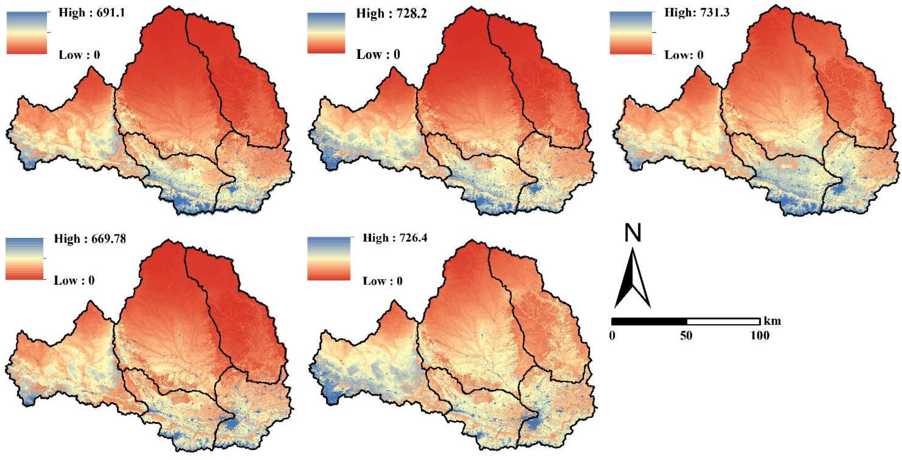
3.1. Simulated Spatiotemporal Patterns of Water Yield in WRB

The interannual changes in precipitation, actual evapotranspiration, and water yield are shown in Figure 2. From 2000 to 2020, the maximum and minimum values of precipitation were 455.75 mm in 2020 and 562.21 mm in 2020, respectively, with a mean value of 500.75 mm. According to the linear regression trend test, precipitation has increased by 1.7 mm per year at the 90% confidence level (p = 0.088) over the past 20 years. This suggests that there may be signs of a trend towards wetting throughout the basin. Moreover, the actual evapotranspiration rose on a global scale at a rate of 4.36 mm year−1 (p = 0.085), with values ranging from 418.87 mm to 479.83 mm and a mean of 445.46 mm. The analysis that was described earlier shows that the AET accounts for 88% of the rainfall in the WRB, and the increasing rate in AET is more than quadruple that of the precipitation. There are considerable spatial and temporal variations in water yield services in Figure 2. The average depth of WY for the whole basin is a minimum of 36.89 mm in 2000, peaking at 82.39 mm in 2020, and the overall WY varied from 73 × 108 m3 to 137 × 108 m3, demonstrating a growth from 2000 to 2020 (Figure S2).
From 2000 to 2020, the spatial pattern of WYs shows significant north-south differences (Figure 3), with low values distributed in the semi-arid Loess Plateau region in the north (<50 m3 /hm2), and high values in the northern foothills of the Qinling Mountains (>300 m3 /hm2). At the sub-catchment level, the high-value areas are mainly located in the main channel of the Wei River, while the low-value areas are mainly located in the Jing and Beiluo Rivers. The “stepped” distribution features were quite apparent in the steady decline in the spatial distribution of WYs that occurred as one moved from the south to the north. Over time, the low-value area in the north tends to increase slowly, while the Qinling Mountains in the south tends to decrease slowly. The high-value areas gradually converge towards the Xi’an urban agglomeration, the Baoji Gorge, and the south-western part of the basin.

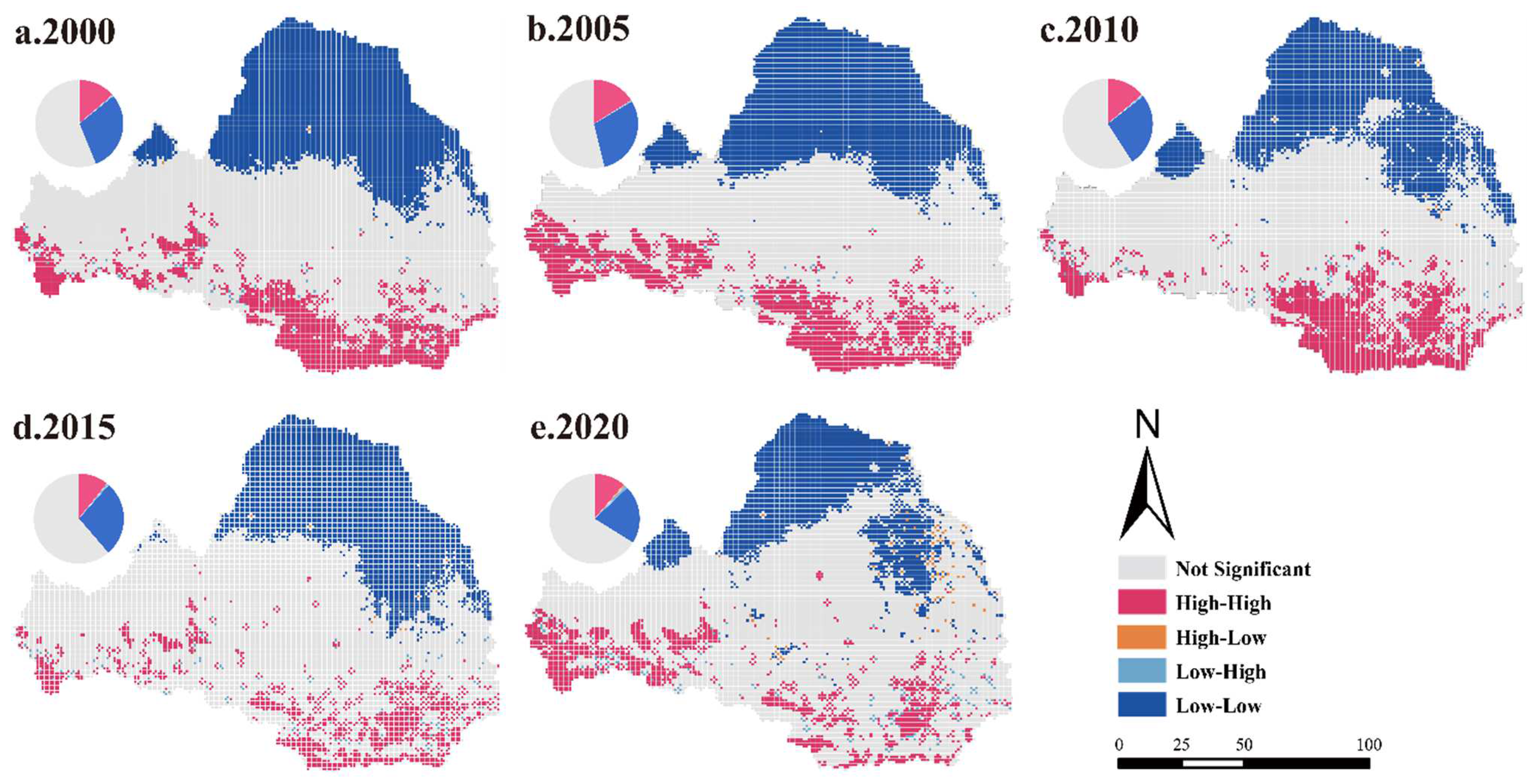
3.2. Identifying the Spatial Dependence of WYs in WRBs

Based on the annual water yield on the grid units from 2000 to 2020, the global spatial autocorrelation results (Moran’s I index) are calculated (Table 3). All of the global Moran’s I values are greater than 0.65, and the p-value is 0.00, which means that the 1% significance level test is successful (Z = 2.58).
This suggests that the spatial distribution of water yield has a positive spatial correlation in the research region, and the geographic clustering phenomena are evident, which meets the prerequisites for the application of the MGWR and GWR models [49]. It can be demonstrated that water yield in the research region is impacted by both environmental and anthropogenic variables. From 2000 to 2005, the difference in Moran’s I has a shifting pattern, ranging from 0.782 to 0.810, before decreasing to 0.686 in 2020. These findings demonstrate that the spatial dependence of water yield in the Wei River basin remains stable.
Analysis of global spatial autocorrelation may only represent the properties of the distribution as a whole, but cannot compute or evaluate the local differences of WYs [4]. Consequently, it is necessary to study the geographical clustering and scatter between the grid units and their surroundings. Four unique forms of local spatial correlations on WYs are depicted on the LISA maps (Figure 4). LL is the main agglomeration type, accounting for more than 20% of the basin and mainly occurring in the semi-arid areas of the Jing and Beiluo river basins. Compared to 2000, the proportion of HH clusters decreased by 5.26% in 2020 and is focused on the southwestern part of the basin and around the Xi’an urban agglomeration. By 2020, the HH/LL clustering of WYs in the study area became more spread out and tended to move toward the line between semi-arid and semi-humid. There is a clear upward trend in the proportion of LH/HL agglomerations, from 0.47% and 0.02% in 2000 to 1.11% and 0.58% in 2020, respectively, mainly around the HH/LL agglomerations.

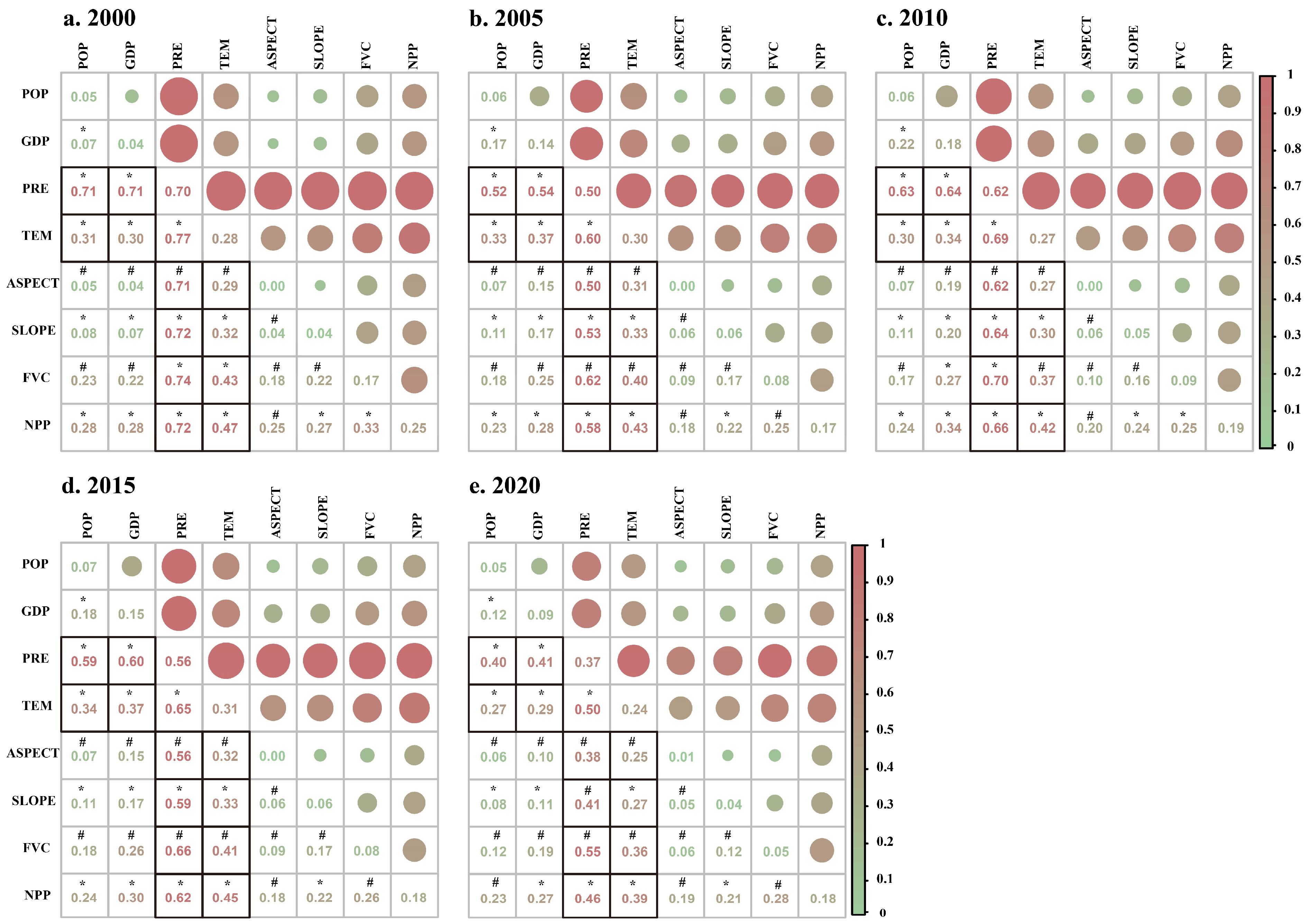
3.3. Analysis of Geodetector Results

3.3.1. Factor Detector Analysis

The explanatory power of different drivers on the spatial differentiation of WYs can be obtained from the factor detector, in the following order of importance: climate factors > vegetative factors > human activities > topographic factors (Table 4), and all the influencing variables passed the significance test (p < 0.01). PRE has the largest degree of effect among the eight examined variables, with q values of 0.703, 0.495, 0.615, 0.56, and 0.371, respectively. The degree of spatial differentiation in the interpretation of WYs by precipitation decreases with time, indicating that the mechanisms that influence the geographical distribution of WYs are getting even more complicated. It is significant to mention that the degree of GDP on WYs is larger than that of POP, in the same trend as the correlation coefficients; the gradual increase in the value of human activity q indicates that the impact of human activity and urbanization on WYs is becoming more pronounced. The onset of the “Anthropocene” signifies that the influence of human activities on the natural environment has significantly surpassed that of natural repair [50]. This is mainly because the increase in POP and GDP is usually indicative of hyperactive anthropogenic activities during city expansion, leading to a significant rise in built-up land and impervious area, which decreases evapotranspiration and precipitation infiltration, hence boosting water supply. There is also a greater difference between the q values of the various influencing variables than there is between the correlation coefficients (Figure S5), indicating that the linear effect dominates the influence on WYs of each factor, and that the non-linear effect of environment variables outweighs the impact of human activities [51].

3.3.2. Interaction Detector Analysis

Among the eight selected possible factors, interaction detectors were used to determine the interactive effects between different variables on the spatial differentiation of WYs (Figure 5). During the period 2000–2020, the analysis showed that there are two different categories of interactions among both pairs of influential variables: two-factors enhancements and non-linear enhancement. As illustrated in Figure 5, the interactions between the factors are dominated by two-factors enhancements. Over time, the number of non-linearly enhanced factor pairs gradually increased from 10 pairs in 2000 to 15 pairs in 2020, with the increase being mainly in FVC and NPP. The relationship between FVC and other factors was limited, while each factor’s influence increased.
The interplay of human, climatic, plant, and terrain variables has a substantially higher influence than most single factors on the geographical differentiation of WYs. Most of the explanatory power of climate factors (including temperature and precipitation) superimposed on other factors is above 0.4. Of these, strong interactions (p > 0.5) of precipitation with other factors occur most frequently. Human activity (both POP and GDP) interacts most strongly with precipitation (shown in the black box in Figure 5), probably because population and GDP are always concentrated in urban areas, reducing the amount of precipitation infiltration. Among all the factors, meteorological variables continue to be the most influential in the variation of WYs. The interplay of meteorological elements (PRE and TEM) controlled the spatial differentiation of the WYs, while POP and GDP derived from anthropogenic activities, combined with meteorological conditions, further affected WYs. However, the number of strong interactions (p > 0.5) between the different factors decreases sharply over time, and the q-values of the different factors gradually approach each other. The interplay between environmental factors is waning, while the interaction between anthropogenic activities and meteorological factors is reinforcing. With environmental change, this means that the synergistic effect of environmental factors and human activities becomes the main cause of the spatial divergence that dominates WYs. The interaction effect between climatic factors and other factors is not as apparent as human activities. This situation is primarily caused by the fact that the elements relating to topography and vegetation are both more complicated and diversified. Additionally, there are additional factors that may cause the degree of spatial stratified heterogeneity to be cancelled out during their interaction with the climatic conditions [50]. The interaction of vegetation factors (including FVC and NPP) with other factors also has an effect (p > 0.2) on the spatial differentiation of WYs, probably because the drivers also have an effect on the spatial distribution of vegetation.

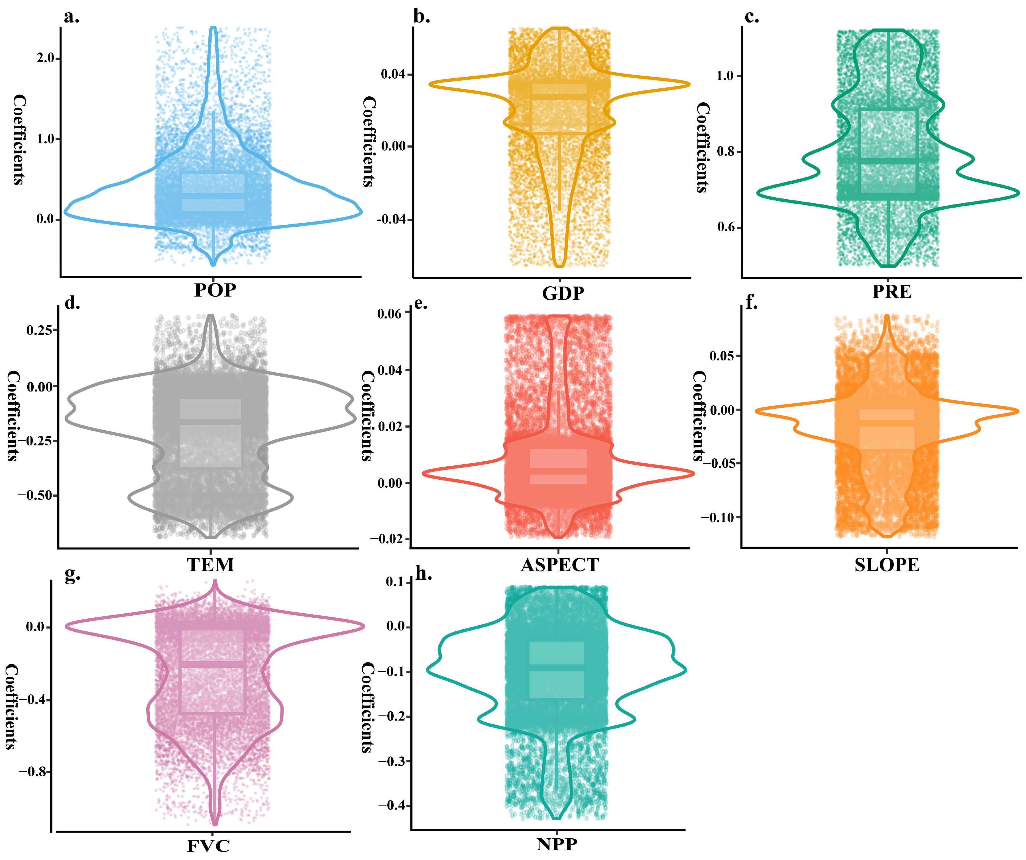
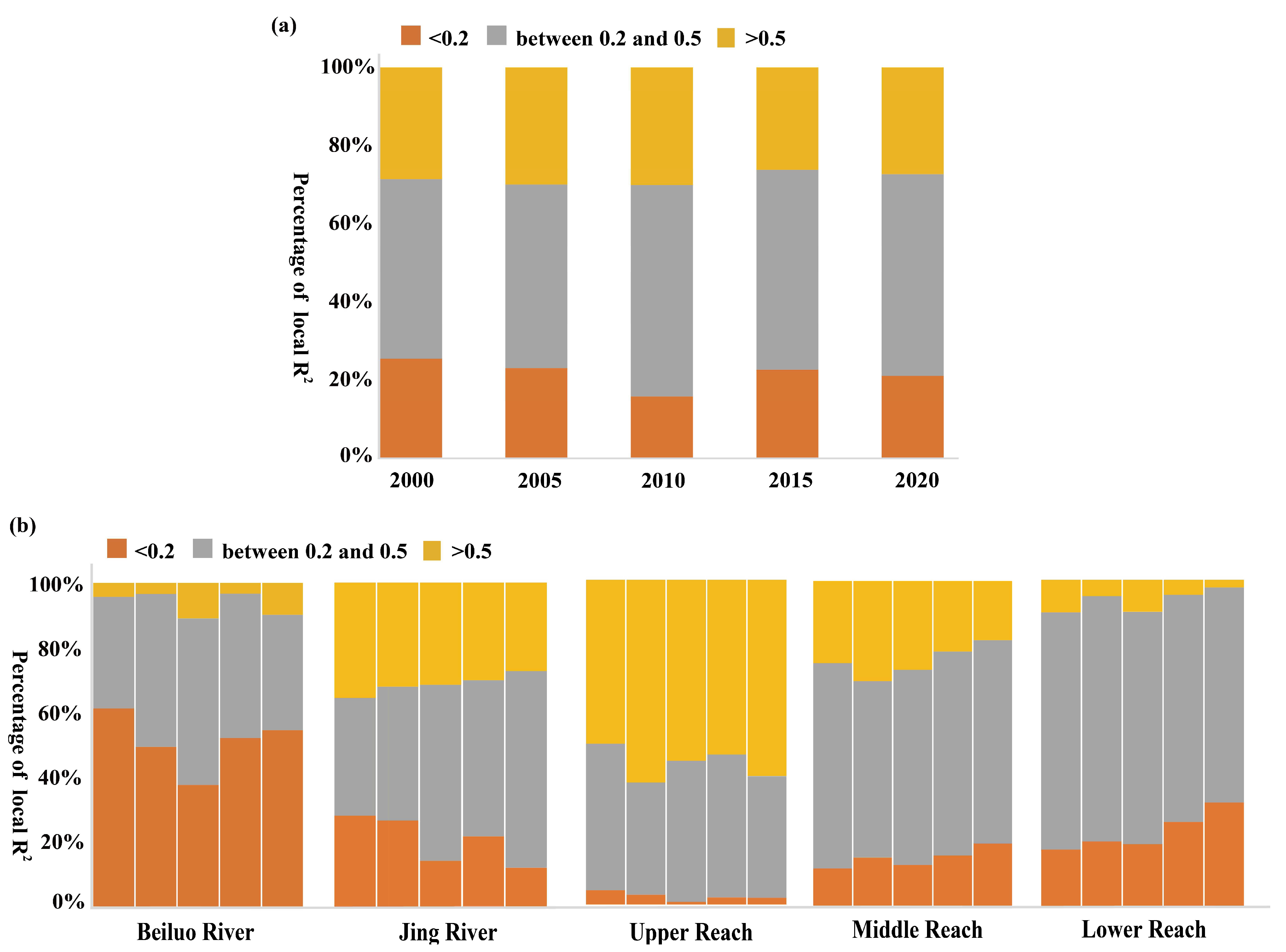
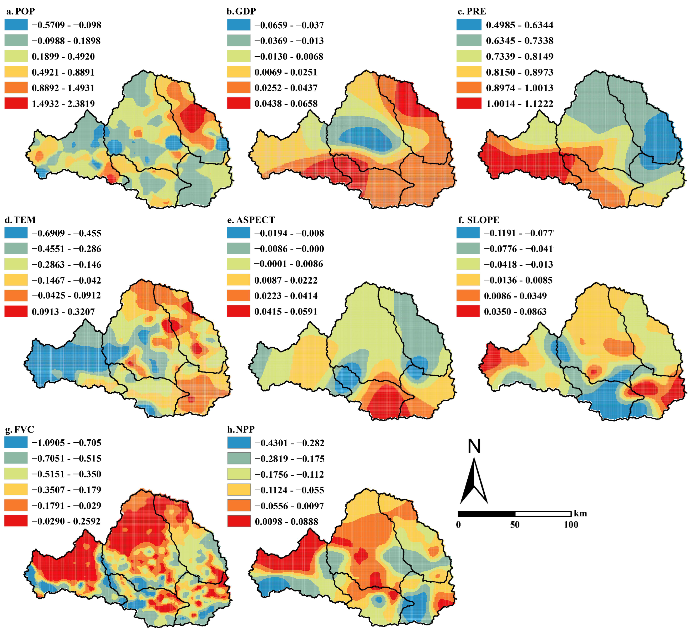
3.4. Multiscale Geographically Weighted Regression Model Analysis

Bandwidth can be seen as the most appropriate sample size for local regression calculations, so the bandwidth in the MGWR model can be thought of as the spatial scale at which the different processes operate. On the one hand, the bandwidth size determines the specific spatial scale (local or global scale) at which the different factors occur; on the other hand, it also determines the potential spatial heterogeneity or spatial stationarity of the relationship between the drivers and WYs. Spatial scales were obtained using the entire number of samples divided by the bandwidth and then rounded up. In order to classify the operational scales of the drivers, the spatial scales are compared with the administrative units at all levels of the Wei River basin and classified as basin scale > sub-basin scale > municipal scale > county scale > local scale.
The MGWR bandwidth for 2000–2020 indicates that each affecting element functions at a different geographical scale (Table 5). It appears that only the county scale and the smaller local scale fluctuated in spatial scale range between 2000 and 2015, suggesting that spatial non-stationarity is unstable and that the county level serves as the primary optimal range for TEM, FVC, and NPP factor. From 2000 to 2020, all factors varied on the same geographical scale and were relatively stable in terms of spatial non-stationarity. Of these, the spatial scale of GDP varied the least, indicating the most stable spatial heterogeneity, probably because the range of variation in GDP has been concentrated in the built-up area. The spatial scale of PRE and slope is the watershed scale, but the fluctuation of slope is more intense and close to the urban scale. Among human activities, the geographical impact range of GDP is the basin scale, which is a global variable. The effect variety of POP is bigger than the effect of population movement, indicating that POP has a significant impact on cross-regional urbanization and water yield services. It is noteworthy that the spatial scale changes of FVC and NPP are opposite, which may be due to the unreasonable structure of the vegetation in the process of returning the land to forest and grass. In general, at smaller local scales, the influence range of natural factors tends to be closer to the size of the country and fluctuates, but the influence range linked with human activities is dominated by large scales and stable.
The regression coefficients from MGWR show how much the drivers affect WYs in different places, and Figure 6 shows the regression coefficients for 2020. Of the regression coefficients for all the factors, only PRE has a single positive effect on WYs, with the other variables often acting in opposite ways across locations. This suggests that the spatial non-stationarity of the distribution of WYs is influenced by different factors at each location. The relatively low regression coefficients for GDP, ASPECT, and SLOPE indicate that they have a limited effect on the spatial heterogeneity of WYs, which is consistent with the previous spatial scale results [51]. The mean values of the regression coefficients for several indicators show that TEM, FVC, and NPP have a relatively strong inhibitory effect on water quantity, while PRE has the largest positive effect on WYs. Given the regression coefficients for human activities, the effect of POP at the county scale is much stronger than for GDP. The range of regression coefficients shows that the order of the main factors influencing the water yield services of WRB is PRE > POP.

4. Discussion

4.1. The MGWR Model Can Precisely Depict the Links among the Drivers Factors and WYs in WRB

Referring to previous studies [39,49], the coefficient of determination (R2), adjusted R2, Akaike information criterion (AIC), and corrected Akaike information criterion (AICc), were chosen in order to evaluate the degree to which the GWR, OLS, and MGWR models matched the data. A greater value of adjusted R2 indicates suggests a perfect match; a lower value of adjusted R2 suggests a worse match. Another measure of model goodness-of-fit is the AICc, which is founded on the principle of entropy; a lower AICc value implies superior predictive accuracy [52,53]. The smaller value of AICc, the more precise the model and the more trustworthy the regression estimation [21]. Comparative analysis reveals that the R2 and adjusted R2 of the MGWR model are significantly higher than those of the OLS and GWR models, while the AICc is significantly lower, indicating that the MGWR model is an effective remedy for the issue of spatial heterogeneity (Table 6). This was previously demonstrated by Hu et al. when they analyzed the model fit effectiveness of OLS, GWR and MGWR in their assessment of ecosystem service drivers [54].
Furthermore, applying Tu’s work [55], we examine whether the MGWR, GWR, and OLS models can account for the spatial autocorrelation of factors by measuring the global Moran’s I of the residuals (Table S3). In this study, there is a strong geographic aggregation phenomenon in the OLS model’s Moran’s I, which varied from 0.2 to 0.3. In contrast, the Moran’s I for the GWR varied from 0.008 to −0.023, effectively eliminating the effect of spatial autocorrelation from the findings. The values of Moran’s I for the MGWR model ranged from −0.003 to −0.023, with values in the MGWR model being significantly less than those in the OLS model and somewhat smaller than those in the GWR model, exhibiting the randomness of the residuals in space. The Moran’s I values for the GWR model varied from slightly larger than −0.023 to a slightly smaller than −0.023. Thus, the MGWR model effectively eliminates the effect of spatial autocorrelation of factors when analyzing the spatial non-stationarity of WYs in the WRB in relation to nature-society, suggesting that the MGWR model is the most dependable of the three.
Wang et al. [56] found that when comparing the performance of the GWR model with the OLS model in terms of describing the linkages between water yield services and natural factors in the Qinling Mountains, the GWR model performed noticeably better than the OLS model. In addition, Liu et al. [52] discovered that the MGWR model was more accurate than the OLS and GWR models when examining the effect of the urban landscape on the land surface temperature in Wuhan. Furthermore, Li et al. [57] launched an investigation into the geographical variability of ecosystem services and discovered that the GWR model can be effective in dealing with the heterogeneity of spatial variables.

4.2. Differences in Local R2 between Basins

There were significant spatial and temporal disparities in the relationship between WYs and impact factors at the catchment scale. The local R2 suggests that MGWR’s predictive power varies geographically [40]. At the basin-wide scale, the proportion of WYs and impact factors significantly correlated (local R2 > 0.2), first increased and then decreased, with a maximum value of 84.2% in 2015 (Figure 7a), which is consistent with the trend of adjusted R2 (Table 4). Of these, those with a strong relationship between WYs and drivers (local R2 between 0.2 and 0.5) ranged from 46% to 54%. In contrast, less than 30% of those had a strong relationship (local R2 > 0.5). At the sub-basin level, the influence of drivers on WYs is mainly concentrated in the upper reaches, where local R2 > 0.5 accounts for more than 50% (Figure 7b). In comparison, the influence of the Beiluo River and Jing River basins in the Loess Plateau region and the downstream where human activities are closely linked is relatively small, with local R2 > 0.5 accounting for less than 10% in the Beiluo River and downstream areas.
The reasons for the differences are probably mainly due to climatic, human activity, and vegetation factors. For the upper reaches, which are in the climatic divide, precipitation is regarded to be one of key elements impacting water yield. The high precipitation and low temperatures in the upper Wei River region may result in lower actual evapotranspiration compared to the Beiluo and Jing River basins. Meanwhile, midstream and downstream climatic conditions are generally consistent, with local R2 showing high explanatory power in the less anthropogenic midstream region (local R2 > 0.5~20%) and low explanatory power in the more anthropogenic downstream region (local R2 > 0.5~6%). This relationship is more complex in catchments in different climatic zones, for example the selected drivers differ significantly in the Beiluo (local R2 < 0.2 at ~50%) and downstream (local R2 < 0.2 at ~20%), so additional factors may be required to accurately explain the regional variability of water supply in different climatic zones. Local R2 mapping is beneficial since this information may be utilized to determine whether regions require additional explanatory factors to better comprehend the underlying mechanisms affecting WYs [58].

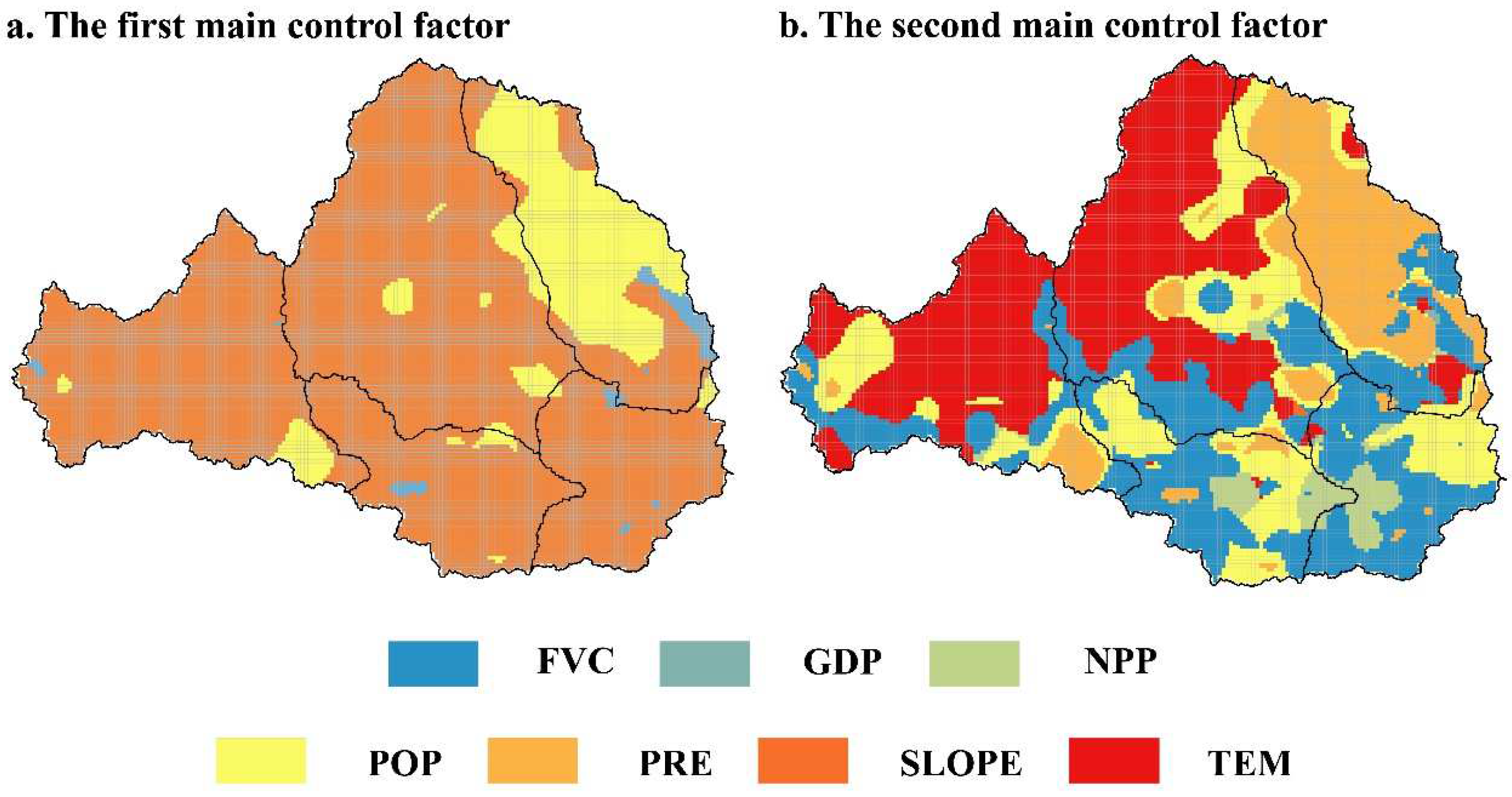
4.3. Drivers of WYs in WRB

The spatial heterogeneity of the association between drivers and WYs is addressed by obtaining regression coefficients for individual factors in different geographical spaces through MGWR. In this section, the output coefficients of the MGWR model in 2020 are used as an example to explore the spatial effects of each driver of WYs in the Wei River basin.
Based on the driving variables’ regression coefficients’ results, we discovered that there were significant differences between natural factors and human activities on WYs in different regions (i.e., spatially non-stationary), and these variables exhibit geographic instability and spatial aggregation (Figure 8). In terms of the range of influence, the range of GDP, PRE, and ASPECT are significantly greater than the other factors. In terms of the direction of influence, there is only a unidirectional effect of precipitation, and the other factors have positive and negative spatial non-smoothness on WYs across the basin. The degree of influence at the basin-wide scale is determined by the mean of the absolute values of the factors’ coefficients, and the sequence of strength of each variable on WYs is PRE > POP > FVC > TME > NPP > SLOPE > ASPECT > GDP.
The two factors with the highest absolute coefficient values at each site were deemed to be the most influential at that location [51]. Figure 9 depicts the spatial non-stationarity of the determinants in WRB, with different colors representing different variables. In terms of space governed by dominating elements, meteorology, population (POP), vegetation cover (FVC), and NPP are the factors of particular concern for the WRB. In addition, meteorological factors were observed to be the main factors dominating the rivers in the semi-arid region (such as the Jing and Beiluo rivers and the upper reaches of the Wei River) and vegetation factors were the main factors dominating the Guanzhong Basin (the middle and lower reaches of the Wei River) (Figure 9b). The geographical distribution of the primary controlling variables only distinguishes the intensity of spatial relationships between various natural and socio-economic factors and identifies the key factors influencing WYs from the perspective of spatial non-stationarity, without the ability to investigate the interplay between several variables.
The distribution patterns of WY show a trend of a stepwise increase from north to south (Figure 3). Our results suggest that WYs in the WRB are strongly influenced by both environmental variables and anthropogenic activities. This is similar to earlier research showing the crucial influence of meteorological factors, human activities, vegetation factors, and topographic features in influencing WYs [13,54,59]. Precipitation is the major factor influencing water yield in the WRB, with coefficient values increasing sequentially from northeast to southwest (Figure 8c). Previous studies [20,60,61] have shown that increasing precipitation is the most significant factor as it significantly impacts water magnitude and terrestrial hydrological processes. Thus, much of the basin-wide water yield is attributable to the influence of changing climate on regional precipitation [62] (Figure 9a). In addition, rising temperatures alter the basin energy balance, affecting precipitation and evapotranspiration patterns [63], which leads to changes in runoff, peak flows, and recharge [59]. The dominant factor in WYs in the upper and Jing River basins is attributed to temperature (Figure 8d), which may be due to low vegetation cover and high evaporation from bare ground in the upper and Jing River basins [64]. Climate change can impact the distribution of WYs by affecting hydrological processes and energy balance [65]. Climate change can therefore affect water yield by altering precipitation and temperature in river basins.
Since 2000, the Wei River basin, especially the Guanzhong basin, has experienced unprecedented land-use change [66]. The expanding of cities is considered to be a crucial element in increasing water yield, while areas with high urbanization show a significant concentration of high WYs (Figure 3). Urban areas may influence water yield in the following ways: (i) heat island effects due to urbanization may alter precipitation and evapotranspiration patterns [67] and (ii) increased impervious surfaces may reduce infiltration of surface runoff [68] and urban evapotranspiration [69]. The population factor (POP) has a positive effect in the North Luo River basin (Figure 8a), at the upstream-lower junction, and a negative effect in the other basins, agreeing with Qi et al. [59]. This may be due to the initial stage of urbanization, which significantly increases water quantity by changing the permeability of the surface. As the level of urbanization increases, human activity negatively affects water yield through increased water use. In addition, the average coefficient of GDP in the WRB is consistently the weakest of all drivers (Figure 8b). The potential reason for this may be that GDP is always focused in the built-up areas and, because of its increase, does not directly affect the water quantity [70].
Within the study area, the influence of geomorphic factors on water yield had an effect over a relatively wide range and to a lesser extent (Figure 8e, f), similar to the previous studies of Hu et al. [18]. In contrast to Hu et al.’s findings, WYs and vegetation factors were significantly negatively correlated in this study, while the extent and impact of FVC and NPP were significantly different. The positive correlation between FVC in the northern part of the semi-arid watershed may be because an appropriate increase in mixed forests and shrublands is effective in reducing evapotranspiration in the semi-arid zone. At the same time, in arid and semi-arid areas, high levels of forest aggregation reduce water quantity by accelerating water depletion and increasing precipitation retention by the tree canopy, which explains the apparent negative correlation in the south-western part of the upper reaches, at the junction of the upper and middle reaches, and in the southern part of the Beiluo River [71].

4.4. Limitations and Future Work Directions

There are certain to be some shortcomings in this study. Uncertainties in the InVEST model predictions are due to a range of simplified presumptions about intricate socio-ecological processes (based on the Budyko hydrological framework) and the climate input errors (especially annual precipitation) [72]. The climate data utilized in this investigation were obtained by interpolating actual observations, and although data quality controls were performed in the data processing, the spatial heterogeneity of meteorological variables prevented the interpolated data from presenting local microclimates [73]. In addition, our study visualizes differences in the relationship between different sub-basins and WYs, with the selected drivers varying dramatically in explanatory power across sub-basins (Figure 7), for example, not explaining well the drivers of WYs in the Beiluo Basin. Although this study used the geographical detector to analyze the interactions between factors, future consideration should be given to how multivariate interactions affect water yield [64].
In future studies, we can use additional hydrological models, including the Lumped Zhang model [36] and the soil and water assessment tool (SWAT) model [74] for comparative studies. Meanwhile, we will use meteorological data with finer spatial resolution and greater accuracy to model water yield [75,76,77,78] and more detailed socio-economic data and landscape characteristics to gain a much broad knowledge of the drivers of WYs in different climatic zones. In addition, multiple validation of linear and non-linear relationships of WYs influences (such as considering both geographic probes and automatic linear modelling (ALM) [13]) to explore synergistic and trade-off effects of natural-social factors would be an important research direction.

5. Conclusions

Understanding the causes of WYs and their relationships in a geospatial context is fundamental, and a prerequisite for ecosystem governance and watershed sustainability. In this study, we assessed the spatial distribution and trends of WYs in the WRB from 2000 to 2020 and quantified the impact of environmental factors on WYs. The results show that from 2000 to 2020, there were clear spatial and temporal differences in water yield, with a slow upward trend and distinct and different spatial aggregation along the climatic divide, with the majority of the growth in water quantity occurring in the metropolitan agglomerations of the WRB. Generally, natural factors have a stronger influence on WYs than anthropogenic activities, and dominate the spatial pattern of WYs. The interactions between driving factors have a significantly larger influence on the spatial variability of WYs than most single factors, and bivariate enhancement and non-linear enhancement predominate among the forms of interaction between components, which demonstrates that there are significant interactions between environmental factors and human activities. Meanwhile, the substantial effect of natural elements is decreasing over time, while the influence of anthropogenic activities is increasing, and the contribution of human activities to WYs must be considered. The results of the spatial regression model show that MGWR provides an excellent model performance in terms of handling with geographical non-stationarity and spatial autocorrelation compared to other regional or global regression models. Specifically, the drivers are strongly correlated with WYs and there is a discernible split in how correlation and strength vary across different geographic locations. Climatic factors (including precipitation and temperature) were the main drivers of WYs in the semi-arid zone, while precipitation and vegetation factors were the main drivers of WYs in the semi-humid zone. In addition, studies have confirmed that appropriate increases in suitable native vegetation in semi-arid zones can effectively increase water supply in semi-arid zones. Policy makers can develop local water management measures for ecosystem services that are tailored to specific local circumstances based on the global and local spatial non-stationarity of WYs’ response to natural society.

Supplementary Materials

The following supporting information can be downloaded at: https://0-www-mdpi-com.brum.beds.ac.uk/article/10.3390/rs14205078/s1, Figure S1. Comparison and validation diagram of model simulation value and observed value; Figure S2. The slopes of changes in precipitation and temperature from 2000-2020; Figure S3. Land-cover types in the Wei River Basin from 2000 to 2020; Figure S4. Soil types in the Wei River Basin; Figure S5. Correlations of WYs in 2000–2020 with driving factors. Pearson correlation is shown in a color gradient (***, p < 0.001; **, p < 0.01; *, p < 0.05); Table S1. The biophysical coefficients table; Table S2. Multicollinearity test between driving variables. Take the year 2000; Table S3. Moran’s I of the residuals of the MGWR, GWR, and OLS models.

Author Contributions

Writing—original draft, Z.C.; conceptualization, P.L.; supervision—methodology, P.L., W.Z., S.W. and Z.T.; writing—review and editing, Y.Z. and B.G. All authors have read and agreed to the published version of the manuscript.

Funding

This study is supported by National Key R&D Program of China (2018YFE0103800), China Scholarship Council (Grant No.: Liujinmei [2022] No. 45), International Education Research Program of Chang’an University (300108221102), General Project of Shaanxi Provincial Key R&D Program—Social Development Field (2021SF-454), GDAS Special Project of Science and Technology Development (2020GDASYL-20200102013), Guangdong Foundation for Program of Science and Technology Research (2019QN01L682) and Asia-Pacific Network for Global Change Research APN project (CRRP2020-03MY-He).

Data Availability Statement

No new data were created or analyzed in this study. Data sharing is not applicable to this article.

Conflicts of Interest

The authors declare no conflict of interest.

References

  1. Costanza, R.; d’Arge, R.; De Groot, R.; Farber, S.; Grasso, M.; Hannon, B.; Limburg, K.; Naeem, S.; O’neill, R.V.; Paruelo, J. The value of the world’s ecosystem services and natural capital. Nature 1997, 387, 253–260. [Google Scholar] [CrossRef]
  2. Costanza, R.; De Groot, R.; Braat, L.; Kubiszewski, I.; Fioramonti, L.; Sutton, P.; Farber, S.; Grasso, M. Twenty years of ecosystem services: How far have we come and how far do we still need to go? Ecosyst. Serv. 2017, 28, 1–16. [Google Scholar] [CrossRef]
  3. Peng, J.; Tian, L.; Zhang, Z.; Zhao, Y.; Green, S.M.; Quine, T.A.; Liu, H.; Meersmans, J. Distinguishing the impacts of land use and climate change on ecosystem services in a karst landscape in China. Ecosyst. Serv. 2020, 46, 101199. [Google Scholar] [CrossRef]
  4. Liang, Y.; Hashimoto, S.; Liu, L. Integrated assessment of land-use/land-cover dynamics on carbon storage services in the Loess Plateau of China from 1995 to 2050. Ecol. Indic. 2021, 120, 106939. [Google Scholar] [CrossRef]
  5. Carpenter Stephen, R.; DeFries, R.; Dietz, T.; Mooney Harold, A.; Polasky, S.; Reid Walter, V.; Scholes Robert, J. Millennium Ecosystem Assessment: Research Needs. Science 2006, 314, 257–258. [Google Scholar] [CrossRef] [PubMed]
  6. Carpenter Stephen, R.; Mooney Harold, A.; Agard, J.; Capistrano, D.; DeFries Ruth, S.; Díaz, S.; Dietz, T.; Duraiappah Anantha, K.; Oteng-Yeboah, A.; Pereira Henrique, M.; et al. Science for managing ecosystem services: Beyond the Millennium Ecosystem Assessment. Proc. Natl. Acad. Sci. USA 2009, 106, 1305–1312. [Google Scholar] [CrossRef] [Green Version]
  7. Perrings, C.; Duraiappah, A.; Larigauderie, A.; Mooney, H. The biodiversity and ecosystem services science-policy interface. Science 2011, 331, 1139–1140. [Google Scholar] [CrossRef]
  8. Cao, Z.; Wang, S.; Luo, P.; Xie, D.; Zhu, W. Watershed Ecohydrological Processes in a Changing Environment: Opportunities and Challenges. Water 2022, 14, 1502. [Google Scholar] [CrossRef]
  9. Yang, Q.; Liu, G.; Casazza, M.; Dumontet, S.; Yang, Z. Ecosystem restoration programs challenges under climate and land use change. Sci. Total Environ. 2022, 807, 150527. [Google Scholar] [CrossRef]
  10. Ma, T.; Sun, S.; Fu, G.; Hall, J.W.; Ni, Y.; He, L.; Yi, J.; Zhao, N.; Du, Y.; Pei, T.; et al. Pollution exacerbates China’s water scarcity and its regional inequality. Nat. Commun. 2020, 11, 650. [Google Scholar] [CrossRef]
  11. Vanham, D.; Hoekstra, A.Y.; Wada, Y.; Bouraoui, F.; De Roo, A.; Mekonnen, M.; Van De Bund, W.; Batelaan, O.; Pavelic, P.; Bastiaanssen, W.G. Physical water scarcity metrics for monitoring progress towards SDG target 6.4: An evaluation of indicator 6.4. 2 “Level of water stress”. Sci. Total Environ. 2018, 613, 218–232. [Google Scholar] [CrossRef] [PubMed]
  12. Fan, M.; Shibata, H.; Chen, L. Spatial conservation of water yield and sediment retention hydrological ecosystem services across Teshio watershed, northernmost of Japan. Ecol. Complex. 2018, 33, 1–10. [Google Scholar] [CrossRef]
  13. Zhang, X.; Zhang, G.; Long, X.; Zhang, Q.; Liu, D.; Wu, H.; Li, S. Identifying the drivers of water yield ecosystem service: A case study in the Yangtze River Basin, China. Ecol. Indic. 2021, 132, 108304. [Google Scholar] [CrossRef]
  14. Vigerstol, K.L.; Aukema, J.E. A comparison of tools for modeling freshwater ecosystem services. J. Environ. Manag. 2011, 92, 2403–2409. [Google Scholar] [CrossRef]
  15. Li, Y.; Yao, S.; Deng, Y.; Jia, L.; Hou, M.; Gong, Z. Spatio-Temporal Study on Supply and Demand Matching of Ecosystem Water Yield Service—A Case Study of Wei River Basin. Pol. J. Environ. Stud. 2021, 30, 1677–1693. [Google Scholar] [CrossRef]
  16. Zhang, Y.; Zhang, B.; Ma, B.; Yao, R.; Wang, L. Evaluation of the water conservation capacity of the Weihe River Basin based on the Integrated Valuation of Ecosystem Services and Tradeoffs model. Ecohydrology 2022, 2022, e2465. [Google Scholar] [CrossRef]
  17. Sun, X.; Guo, H.; Lian, L.; Liu, F.; Li, B. The spatial pattern of water yield and its driving factors in Nansi Lake basin. J. Nat. Resour. 2017, 32, 669–679. [Google Scholar]
  18. Hao, R.; Yu, D.; Liu, Y.; Liu, Y.; Qiao, J.; Wang, X.; Du, J. Impacts of changes in climate and landscape pattern on ecosystem services. Sci. Total Environ. 2017, 579, 718–728. [Google Scholar] [CrossRef]
  19. Dai, E.; Wang, Y. Spatial heterogeneity and driving mechanisms of water yield service in the Hengduan Mountain region. Acta Geogr. Sin. 2020, 75, 607–619. [Google Scholar]
  20. Hoyer, R.; Chang, H. Assessment of freshwater ecosystem services in the Tualatin and Yamhill basins under climate change and urbanization. Appl. Geogr. 2014, 53, 402–416. [Google Scholar] [CrossRef]
  21. Fotheringham, A.S.; Yang, W.; Kang, W. Multiscale geographically weighted regression (MGWR). Ann. Am. Assoc. Geogr. 2017, 107, 1247–1265. [Google Scholar] [CrossRef]
  22. Yu, H.; Fotheringham, A.S.; Li, Z.; Oshan, T.; Kang, W.; Wolf, L.J. Inference in Multiscale Geographically Weighted Regression. Geogr. Anal. 2020, 52, 87–106. [Google Scholar] [CrossRef]
  23. Bennett, E.M.; Peterson, G.D.; Gordon, L.J. Understanding relationships among multiple ecosystem services. Ecol. Lett. 2009, 12, 1394–1404. [Google Scholar] [CrossRef] [PubMed]
  24. Wu, C.; Qiu, D.; Gao, P.; Mu, X.; Zhao, G. Application of the InVEST model for assessing water yield and its response to precipitation and land use in the Weihe River Basin, China. J. Arid Land 2022, 14, 426–440. [Google Scholar] [CrossRef]
  25. Yang, J.; Xie, B.P.; Zhang, D.G. Spatio-temporal variation of water yield and its response to precipitation and land use change in the Yellow River Basin based on InVEST model. J. Appl. Ecol. 2020, 31, 2731–2739. [Google Scholar]
  26. Jiang, C.; Li, D.Q.; Wang, D.W.; Zhang, L.B. Quantification and assessment of changes in ecosystem service in the Three-River Headwaters Region, China as a result of climate variability and land cover change. Ecol. Indic. 2016, 66, 199–211. [Google Scholar] [CrossRef]
  27. Yang, M.; Gao, X.; Zhao, X.; Wu, P. Scale effect and spatially explicit drivers of interactions between ecosystem services—A case study from the Loess Plateau. Sci. Total Environ. 2021, 785, 147389. [Google Scholar] [CrossRef]
  28. Zhu, Y.; Luo, P.; Zhang, S.; Sun, B. Spatiotemporal analysis of hydrological variations and their impacts on vegetation in semiarid areas from multiple satellite data. Remote Sens. 2020, 12, 4177. [Google Scholar] [CrossRef]
  29. Qiu, D.; Wu, C.; Mu, X.; Zhao, G.; Gao, P. Changes in extreme precipitation in the Wei River Basin of China during 1957–2019 and potential driving factors. Theor. Appl. Climatol. 2022, 149, 915–929. [Google Scholar] [CrossRef]
  30. Liu, J.; Xia, J.; She, D.; Li, L.; Wang, Q.; Zou, L. Evaluation of six satellite-based precipitation products and their ability for capturing characteristics of extreme precipitation events over a climate transition area in China. Remote Sens. 2019, 11, 1477. [Google Scholar] [CrossRef] [Green Version]
  31. Li, C.; Zhang, H.; Gong, X.; Wei, X.; Yang, J. Precipitation trends and alteration in Wei River Basin: Implication for water resources management in the transitional zone between plain and loess plateau, China. Water 2019, 11, 2407. [Google Scholar] [CrossRef] [Green Version]
  32. 2022 New Urbanization and Key Tasks of Urban-Rural Integration Development. Available online: https://www.ndrc.gov.cn/xxgk/zcfb/tz/202203/t20220317_1319455.html?code=&state=123 (accessed on 20 May 2022).
  33. Yang, J.; Huang, X. The 30 m annual land cover dataset and its dynamics in China from 1990 to 2019. Earth Syst. Sci. Data 2021, 13, 3907–3925. [Google Scholar] [CrossRef]
  34. InVEST 3.2.0 User‘s Guide. Available online: http://naturalcapitalproject-stanford-edu-s.vpn.chd.edu.cn:8080/software/invest (accessed on 16 March 2022).
  35. Fu, B. On the calculation of the evaporation from land surface. Sci. Atmos. Sin. 1981, 5, 23–31. [Google Scholar]
  36. Zhang, L.; Hickel, K.; Dawes, W.; Chiew, F.H.; Western, A.; Briggs, P. A rational function approach for estimating mean annual evapotranspiration. Water. Resour. Res. 2004, 40, W02502. [Google Scholar] [CrossRef]
  37. Hargreaves, G.H.; Allen, R.G. History and evaluation of Hargreaves evapotranspiration equation. J. Irrig. Drain. Eng. 2003, 129, 53–63. [Google Scholar] [CrossRef]
  38. Deng, C.; Zhu, D.; Nie, X.; Liu, C.; Zhang, G.; Liu, Y.; Li, Z.; Wang, S.; Ma, Y. Precipitation and urban expansion caused jointly the spatiotemporal dislocation between supply and demand of water provision service. J. Environ. Manag. 2021, 299, 113660. [Google Scholar] [CrossRef]
  39. Zhao, H.; Liu, Y.; Gu, T.; Zheng, H.; Wang, Z.; Yang, D. Identifying Spatiotemporal Heterogeneity of PM2.5 Concentrations and the Key Influencing Factors in the Middle and Lower Reaches of the Yellow River. Remote Sens. 2022, 14, 2643. [Google Scholar] [CrossRef]
  40. Lei, C.; Wang, Q.; Wang, Y.; Han, L.; Yuan, J.; Yang, L.; Xu, Y. Spatially non-stationary relationships between urbanization and the characteristics and storage-regulation capacities of river systems in the Tai Lake Plain, China. Sci. Total Environ. 2022, 824, 153684. [Google Scholar] [CrossRef]
  41. Getis, A. Spatial autocorrelation. In Handbook of Applied Spatial Analysis; Springer: Berlin/Heidelberg, Germany, 2010; pp. 255–278. [Google Scholar]
  42. Anselin, L.; Rey, S.J. Modern Spatial Econometrics in Practice: A Guide to GeoDa, GeoDaSpace and PySAL; GeoDa Press LLC: Chicago, IL, USA, 2014; pp. 30–121. [Google Scholar]
  43. Wang, J.-F.; Zhang, T.-L.; Fu, B.-J. A measure of spatial stratified heterogeneity. Ecol. Indic. 2016, 67, 250–256. [Google Scholar] [CrossRef]
  44. Zhao, R.; Zhan, L.; Yao, M.; Yang, L. A geographically weighted regression model augmented by Geodetector analysis and principal component analysis for the spatial distribution of PM2.5. Sustain. Cities Soc. 2020, 56, 102106. [Google Scholar] [CrossRef]
  45. Wang, J.-F.; Hu, Y. Environmental health risk detection with GeogDetector. Environ. Model. Softw. 2012, 33, 114–115. [Google Scholar] [CrossRef]
  46. Wang, C.; Wang, J.; Naudiyal, N.; Wu, N.; Cui, X.; Wei, Y.; Chen, Q. Multiple Effects of Topographic Factors on Spatio-Temporal Variations of Vegetation Patterns in the Three Parallel Rivers Region, Southeast Qinghai-Tibet Plateau. Remote Sens. 2022, 14, 151. [Google Scholar] [CrossRef]
  47. Oshan, T.M.; Li, Z.; Kang, W.; Wolf, L.J.; Fotheringham, A.S. Mgwr: A Python implementation of multiscale geographically weighted regression for investigating process spatial heterogeneity and scale. ISPRS Int. J. Geoinf. 2019, 8, 269. [Google Scholar] [CrossRef] [Green Version]
  48. Li, Z.; Fotheringham, A.S. Computational improvements to multi-scale geographically weighted regression. Int. J. Geogr. Inform. Sci. 2020, 34, 1378–1397. [Google Scholar] [CrossRef]
  49. Wang, L.; Wang, S.; Zhou, Y.; Liu, W.; Hou, Y.; Zhu, J.; Wang, F. Mapping population density in China between 1990 and 2010 using remote sensing. Remote Sens. Environ. 2018, 210, 269–281. [Google Scholar] [CrossRef]
  50. Waters, C.N.; Zalasiewicz, J.; Summerhayes, C.; Barnosky, A.D.; Poirier, C.; Gałuszka, A.; Cearreta, A.; Edgeworth, M.; Ellis, E.C.; Ellis, M. The Anthropocene is functionally and stratigraphically distinct from the Holocene. Science 2016, 351, aad2622. [Google Scholar] [CrossRef] [PubMed]
  51. Wu, T.; Zhou, L.; Jiang, G.; Meadows, M.E.; Zhang, J.; Pu, L.; Wu, C.; Xie, X. Modelling Spatial Heterogeneity in the Effects of Natural and Socioeconomic Factors, and Their Interactions, on Atmospheric PM2.5 Concentrations in China from 2000–2015. Remote Sens. 2021, 13, 2152. [Google Scholar] [CrossRef]
  52. Liu, H.; Zhan, Q.; Gao, S.; Yang, C. Seasonal Variation of the Spatially Non-Stationary Association Between Land Surface Temperature and Urban Landscape. Remote Sens. 2019, 11, 1016. [Google Scholar] [CrossRef] [Green Version]
  53. Niu, L.; Zhang, Z.; Peng, Z.; Liang, Y.; Liu, M.; Jiang, Y.; Wei, J.; Tang, R. Identifying Surface Urban Heat Island Drivers and Their Spatial Heterogeneity in China’s 281 Cities: An Empirical Study Based on Multiscale Geographically Weighted Regression. Remote Sens. 2021, 13, 4428. [Google Scholar] [CrossRef]
  54. Hu, B.; Kang, F.; Han, H.; Cheng, X.; Li, Z. Exploring drivers of ecosystem services variation from a geospatial perspective: Insights from China’s Shanxi Province. Ecol. Indic. 2021, 131, 108188. [Google Scholar] [CrossRef]
  55. Tu, J. Spatially varying relationships between land use and water quality across an urbanization gradient explored by geographically weighted regression. Appl. Geogr. 2011, 31, 376–392. [Google Scholar] [CrossRef]
  56. Wang, X.; Fu, X.; Chu, B.; Li, Y.; Yan, Y.; Feng, X. Spatio-temporal variation of water yield and its driving factors in Qinling Mountains barrier region. J. Nat. Resour. 2021, 36, 2507–2521. [Google Scholar] [CrossRef]
  57. Li, C.; Zhao, J. Investigating the spatiotemporally varying correlation between urban spatial patterns and ecosystem services: A case study of Nansihu Lake Basin, China. ISPRS Int. J. Geoinf. 2019, 8, 346. [Google Scholar] [CrossRef] [Green Version]
  58. Tran, D.X.; Pearson, D.; Palmer, A.; Lowry, J.; Gray, D.; Dominati, E.J. Quantifying spatial non-stationarity in the relationship between landscape structure and the provision of ecosystem services: An example in the New Zealand hill country. Sci. Total Environ. 2022, 808, 152126. [Google Scholar] [CrossRef]
  59. Qi, Y.; Lian, X.; Wang, H.; Zhang, J.; Yang, R. Dynamic mechanism between human activities and ecosystem services: A case study of Qinghai lake watershed, China. Ecol. Indic. 2020, 117, 106528. [Google Scholar] [CrossRef]
  60. Goyal, M.K.; Khan, M. Assessment of spatially explicit annual water-balance model for Sutlej River Basin in eastern Himalayas and Tungabhadra River Basin in peninsular India. Hydrol. Res. 2017, 48, 542–558. [Google Scholar] [CrossRef] [Green Version]
  61. Li, J.; Dong, S.; Li, Y.; Wang, Y.; Li, Z.; Li, F. Effects of land use change on ecosystem services in the China–Mongolia–Russia economic corridor. J. Clean. Prod. 2022, 360, 132175. [Google Scholar] [CrossRef]
  62. Legesse, D.; Vallet-Coulomb, C.; Gasse, F. Hydrological response of a catchment to climate and land use changes in Tropical Africa: Case study South Central Ethiopia. J. Hydrol. 2003, 275, 67–85. [Google Scholar] [CrossRef]
  63. Zhu, W.; Wang, S.; Luo, P.; Zha, X.; Cao, Z.; Lyu, J.; Zhou, M.; He, B.; Nover, D. A Quantitative Analysis of the Influence of Temperature Change on the Extreme Precipitation. Atmosphere 2022, 13, 612. [Google Scholar] [CrossRef]
  64. Jiang, Y.; Xu, L.; Yang, G.; Ren, G. Microclimate effects under different forest-grass rehabilitation of vegetation models in summer. Agric. Res. Arid. Areas 2007, 25, 162–174. [Google Scholar]
  65. Wang, S.; Cao, Z.; Luo, P.; Zhu, W. Spatiotemporal Variations and Climatological Trends in Precipitation Indices in Shaanxi Province, China. Atmosphere 2022, 13, 744. [Google Scholar] [CrossRef]
  66. Zhao, Y.; Feng, Q.; Lu, A. Spatiotemporal variation in vegetation coverage and its driving factors in the Guanzhong Basin, NW China. Ecol. Inform. 2021, 64, 101371. [Google Scholar] [CrossRef]
  67. Kaufmann, R.K.; Seto, K.C.; Schneider, A.; Liu, Z.; Zhou, L.; Wang, W. Climate response to rapid urban growth: Evidence of a human-induced precipitation deficit. J. Clim. 2007, 20, 2299–2306. [Google Scholar] [CrossRef]
  68. Suriya, S.; Mudgal, B.V. Impact of urbanization on flooding: The Thirusoolam sub watershed—A case study. J. Hydrol. 2012, 412–413, 210–219. [Google Scholar] [CrossRef]
  69. Chen, H.; Huang, J.J.; Dash, S.S.; McBean, E.; Wei, Y.Z.; Li, H. Assessing the impact of urbanization on urban evapotranspiration and its components using a novel four-source energy balance model. Agric. For. Meteorol. 2022, 316, 108853. [Google Scholar] [CrossRef]
  70. Xu, J.; Liu, S.; Zhao, S.; Wu, X.; Hou, X.; An, Y.; Shen, Z. Spatiotemporal dynamics of water yield service and its response to urbanisation in the Beiyun river Basin, Beijing. Sustainability 2019, 11, 4361. [Google Scholar] [CrossRef] [Green Version]
  71. Cao, S.; Chen, L.; Yu, X. Impact of China’s Grain for Green Project on the landscape of vulnerable arid and semi-arid agricultural regions: A case study in northern Shaanxi Province. J. Appl. Ecol. 2009, 46, 536–543. [Google Scholar] [CrossRef]
  72. Hamel, P.; Guswa, A.J. Uncertainty analysis of a spatially explicit annual water-balance model: Case study of the Cape Fear basin, North Carolina. Hydrol. Earth Syst. Sci. 2015, 19, 839–853. [Google Scholar] [CrossRef] [Green Version]
  73. Asadi Oskouei, E.; Delsouz Khaki, B.; Kouzegaran, S.; Navidi, M.N.; Haghighatd, M.; Davatgar, N.; Lopez-Baeza, E. Mapping Climate Zones of Iran Using Hybrid Interpolation Methods. Remote Sens. 2022, 14, 2632. [Google Scholar] [CrossRef]
  74. Dennedy-Frank, P.J.; Muenich, R.L.; Chaubey, I.; Ziv, G. Comparing two tools for ecosystem service assessments regarding water resources decisions. J. Environ. Manag. 2016, 177, 331–340. [Google Scholar] [CrossRef] [Green Version]
  75. Wang, Y.W.; Zhao, N. Evaluation of Eight High-Resolution Gridded Precipitation Products in the Heihe River Basin, Northwest China. Remote Sens. 2022, 14, 1458. [Google Scholar] [CrossRef]
  76. Luo, P.; Luo, M.; Li, F.; Qi, X.; Huo, A.; Wang, Z.; He, B.; Takara, K.; Nover, D. Urban flood numerical simulation: Research, methods and future perspectives. Environ. Model. Softw. 2022, 105478. [Google Scholar] [CrossRef]
  77. Luo, P.; Zheng, Y.; Wang, Y.; Zhang, S.; Yu, W.; Zhu, X.; Huo, A.; Wang, Z.; He, B.; Nover, D. Comparative Assessment of Sponge City Constructing in Public Awareness, Xi’an, China. Sustainability 2022, 14, 11653. [Google Scholar] [CrossRef]
  78. Luo, P.; Liu, L.; Wang, S.; Ren, B.; He, B.; Nover, D. Influence assessment of new Inner Tube Porous Brick with absorbent concrete on urban floods control. Case Stud. Constr. Mat. 2022, 17, e01236. [Google Scholar] [CrossRef]
Figure 1. Geographical location of the study area and the sub-basins in the WRB. The whole basin is divided into five sub-basins: 1. The Beiluo River; 2. The Jing River; 3. The upper reach of the Wei River basin; 4. The middle reach of the Wei River basin; and 5. The lower reach of the Wei River basin.
Remotesensing 14 05078 g001
Figure 2. Annual precipitation, actual evapotranspiration and water yield service in the Wei River basin from 2000–2020.
Remotesensing 14 05078 g002
Figure 3. Spatial pattern of WYs in Wei River basin from 2000 to 2020.
Remotesensing 14 05078 g003
Figure 4. Univariate LISA maps of WYs in 2000–2020.
Remotesensing 14 05078 g004
Figure 5. The synergistic contribution of potential impact factors to water yield services. * represents bivariate enhancement; # represents non-linear enhancement.
Remotesensing 14 05078 g005
Figure 6. A combined plot of regression coefficients of drivers derived from the MGWR model in 2020. The Centre line is the median; box limits indicate upper and lower quartiles; and the outline displays the distribution of the data. Variables include (a) population density (POP), (b) gross domestic product (GDP), (c) precipitation (PRE), (d) temperature (TEM), (e) aspect (ASPECT), (f) slope (SLOPE), (g) fractional vegetation cover (FVC), (h) net primary productivity (NPP).
Remotesensing 14 05078 g006
Figure 7. Differences in WYs’ Local R2 in the WRB. (a) The differences in the Local R2 in the WRB. (b) The differences in the Local R2 in the sub-basin.
Remotesensing 14 05078 g007
Figure 8. Local spatial distribution of regression coefficients of MGWR model.Variables include (a) population density (POP), (b) gross domestic product (GDP), (c) precipitation (PRE), (d) temperature (TEM), (e) aspect (ASPECT), (f) slope (SLOPE), (g) fractional vegetation cover (FVC), (h) net primary productivity (NPP).
Remotesensing 14 05078 g008
Figure 9. The distribution patterns of primary control variables in disparate positions in WRB. (a) The distribution patterns of the first major control variables; (b) the distribution patterns of the second main control factors.
Remotesensing 14 05078 g009
Table 1. Details about the important data used in this study.
DataMinMaxUnitTypeResolutionSource
Precipitation312.21172.6mmRaster1 kmNational Earth System Science Data Center (http://www.geodata.cn/) (accessed on 16 March 2022)
Temperature−1.715.6°CRaster1 kmNational Earth System Science Data Center (http://www.geodata.cn/) (accessed on 16 March 2022)
Land Use and Land Cover (LULC) data---Raster30 m[33]
DEM2373934mRaster30 mGeospatial Data Cloud (http://www.gscloud.cn) (accessed on 16 March 2022)
Soil Data ---Raster1 kmHarmonized World Soil Database (http://westdc.westgis.ac.cn) (accessed on 16 March 2022)
GDP 2.5537,028.3CNY/km2Raster1 kmResource and Environment Science Data Center, Chinese Academy of Sciences (http://www.resdc.cn/) (accessed on 16 March 2022)
Population 081,139.9People/km2Raster1 kmResource and Environment Science Data Center, Chinese Academy of Sciences (http://www.resdc.cn/) (accessed on 16 March 2022)
FVC01-Raster250 mMODIS (http://modis.gsfc.nasa.gov/) (accessed on 16 March 2022)
NPP77.71164.1-Raster500 mMODIS (http://modis.gsfc.nasa.gov/) (accessed on 16 March 2022)
Table 2. Interaction types of two driving factors.
Judgments BasedType of Interaction
q (X1 ∩ X2) < min(q(X1), q(X2))Non-linear reduction
min(q(X1), q(X2)) < q (X1 ∩ X2) < max(q(X1), q(X2))Single-factor non-linear reduction
q (X1 ∩ X2) > max(q(X1), q(X2))Two-factor enhancement
q (X1 ∩ X2) = q(X1) + q(X2)Independent
q (X1 ∩ X2) > q(X1) + q(X2)Non-linear enhancement
Table 3. Spatial pattern of WYs in the Wei River basin from 2000 to 2020.
YearMoran’s IZ-Scorep-Value
20000.782134.8820.00
20050.810142.3320.00
20100.769140.1610.00
20150.689133.6440.00
20200.686149.4650.00
Table 4. The q value of each driving factors derived from the factor detector.
Factors 20002005201020152020
Human activitiesPOP0.05 **0.063 **0.061 **0.065 **0.05 **
GDP0.039 **0.142 **0.184 **0.148 **0.093 **
Climatic factorsPRE0.703 **0.495 **0.615 **0.56 **0.371 **
TEM0.283 **0.302 **0.267 **0.31 **0.244 **
Topography factorsASPECT0.0014 **0.0027 **0.0027 **0.0027 **0.058 **
SLOPE0.0355 **0.057 **0.054 **0.057 **0.038 **
Vegetative factorsFVC0.173 **0.079 **0.087 **0.079 **0.0456 **
NPP0.246 **0.169 **0.188 **0.176 **0.18 **
** Represents p < 0.01.
Table 5. The bandwidth of all factors obtained from the MGWR model.
Variables20002005201020152020
BW 1NLU 2BWNLUBWNLUBWNLUBWNLU
POP3414434344277542775428054
GDP15,015115,015115,015115,015154303
PRE3597432815401844606319378
TEM70215222681461032645733645
ASPECT17049262963819415,012135994
SLOPE222071317111739820307103714
FVC37940672248916989169100150
NPP10214742635824187771957726
1 Bandwidth spatially for every factor; 2 Spatial scale of occurrence of different factors.
Table 6. Comparative analysis of the MGWR and OLS/GWR models.
R2Adjusted R2AICAICc
2000OLS0.7150.71423,803.25623,805.271
GWR0.8280.81718,168.07718,005.001
MGWR0.8380.82118,471.73318,127.638
2005OLS0.7300.73022,978.37722,980.392
GWR0.8470.83716,320.63616,341.024
MGWR0.8540.84016,220.72116,341.024
2010OLS0.7160.71523,755.31723,757.332
GWR0.8080.79719,522.11319,720.232
MGWR0.8160.80119,462.88319,554.417
2015OLS0.5910.59129,204.39429,206.409
GWR0.7230.70924,772.69824,947.926
MGWR0.7370.71624,782.24024,857.002
2020OLS0.5410.54130,941.70030,943.714
GWR0.6910.67726,302.03926,363.564
MGWR0.7050.68526,209.41226,343.399
Publisher’s Note: MDPI stays neutral with regard to jurisdictional claims in published maps and institutional affiliations.

