Article

Dynamic Modelling of Water and Wind Erosion in Australia over the Past Two Decades

1
School of Life Sciences, Faculty of Science, University of Technology Sydney, Broadway, NSW 2007, Australia
2
Soil and Landscape Science, School of Molecular and Life Sciences, Faculty of Science and Engineering, Curtin University, Perth, WA 6845, Australia
3
NSW Department of Primary Industries, Orange Agricultural Institute, Orange, NSW 2800, Australia
4
Fenner School of Environment and Society, Australian National University, Canberra, ACT 2601, Australia
5
Science, Economics and Insights Division, NSW Department of Planning and Environment, Gunnedah, NSW 2124, Australia
6
Land and Water—Black Mountain, CSIRO, Canberra, ACT 2601, Australia
7
NSW Department of Planning and Environment, Parramatta, NSW 2150, Australia
8
State Key Laboratory of Soil Erosion and Dryland Farming on the Loess Plateau, Institute of Soil and Water Conservation, Northwest A&F University, Xianyang 712100, China
*
Author to whom correspondence should be addressed.
Remote Sens. 2022, 14(21), 5437; https://0-doi-org.brum.beds.ac.uk/10.3390/rs14215437
Submission received: 29 September 2022 / Revised: 21 October 2022 / Accepted: 24 October 2022 / Published: 29 October 2022

Abstract

:
Soil erosion caused by water and wind is a complicated natural process that has been accelerated by human activity. It results in increasing areas of land degradation, which further threaten the productive potential of landscapes. Consistent and continuous erosion monitoring will help identify the location, magnitude, and trends of soil erosion. This information can then be used to evaluate the impact of land management practices and inform programs that aim to improve soil conditions. In this study, we applied the Revised Universal Soil Loss Equation (RUSLE) and the Revised Wind Erosion Equation (RWEQ) to simulate water and wind erosion dynamics. With the emerging earth observation big data, we estimated the monthly and annual water erosion (with a resolution of 90 m) and wind erosion (at 1 km) from 2001 to 2020. We evaluated the performance of three gridded precipitation products (SILO, GPM, and TRMM) for monthly rainfall erosivity estimation using ground-based rainfall. For model validation, water erosion products were compared with existing products and wind erosion results were verified with observations. The datasets we developed are particularly useful for identifying finer-scale erosion dynamics, where more sustainable land management practices should be encouraged.

1. Introduction

Soil erosion is a major threat to the sustainability of agriculture [1,2]. Under changing land use and climate, soil erosion from water and wind has accelerated impacts on economic, social, and environmental systems, both on-site and off-site [3]. Water and wind erosion causes the on-site loss of soil, nutrients, and organic matter, which results in decreased soil fertility and land productivity. About 10 million hectares of cropland worldwide are abandoned annually due to reduced productivity caused by soil erosion [4,5]. This leads to a further reduction in the social viability and population levels in rural communities, influencing long-term sustainable regional development. The subsequent sedimentation and nutrient movement may also cause off-site environmental, air, and water quality degradation [6].
In Australia, the assessment by Bui et al. [7] concluded that soil erosion in Australian cropping regions was occurring at unsustainable rates and has a critical impact on agricultural productivity. Environmental impacts of excessive sedimentation and nutrient delivery on inland waters, estuaries, and coasts are already occurring. The net median erosion rate in cultivated regions is estimated at 1.3 Mg ha−1 yr−1 [8], and 7% of Australia had soil losses of more than 1.0 Mg ha−1 yr−1. It should also be noted that Australia is one of the most fire-prone regions of the world. Wildfire-related water erosion in Australia is responsible for reef deterioration, road damage, and river pollutants [9]. While water erosion is the dominant form of erosion in most parts of Australia, wind erosion is most common in deserts, coastal sand dune environments, and beaches, and certain land conditions cause wind erosion in agricultural areas. Dust storms from arid and semi-arid areas of Australia can travel long distances and affect the air quality in coastal zones where most Australians live [10]. Since 2000, the millennium drought and the mega-fires in Australia have also highlighted the urgent need to revisit soil erosion dynamics to provide a more contemporary view of water and wind erosion trends.
Over the last century, extensive studies have been conducted to estimate soil erosion using various monitoring and modelling approaches. From the perspective of the representation of soil erosion, water and wind erosion models are classified into three groups, viz. empirical, processed-based, and machine learning models [11,12]. Each of these models has found its niche for different reasons. The empirical water erosion model, like the Universal Soil Loss Equation (USLE) and the Revised USLE (RUSLE), is relatively easy to parameterize. The simplicity of these models enables the handling of large datasets and computation, making them attractive for land degradation assessments over large areas. Process-based water erosion models, like the Water Erosion Prediction Project (WEPP) and Griffith University Erosion System Template (GUEST), can provide insights concerning the space-time evolution of the soil erosion processes involved [13,14]. However, the non-linear and physical parameters of processed-based models need to be calibrated by many input observations, and they are hard to apply over large areas. In recent years, large and abundant Earth Observation (EO) datasets have become publicly available to scientists. Rather than using traditional models, big data-based machine-learning (ML) methods (like SVM, RF, ANN) have been successfully used for landslides, debris flows, and gully erosion [15]. While water erosion models were initially developed in agricultural areas, wind erosion models have mainly been applied in drylands where dust originates.
To monitor the wind erosion hazard at a high spatio-temporal resolution, empirical models, like the Revised Wind Equation (RWEQ), process-based models, like the Single-Event Wind Erosion Evaluation Program (SWEEP), and albedo-based models have been developed to assess the spatial and temporal patterns in wind erosion dynamics in various landscapes [16,17,18]. The commonly used RWEQ model has the ability to consider the impacts of weather, soil, vegetation, and roughness factors on the rate of soil loss. Kok et al. [19] describe a physically based wind erosion model. A critical approximation in wind erosion modelling is the momentum extracted by roughness elements, which can be expressed by roughness density lateral cover. The lateral cover underpins current wind erosion models. However, the estimation of lateral cover over large areas is challenging and often approximated by remote sensing vegetation cover. By replacing the use of lateral cover, which closely relates to sheltered area, Chappell et al. [17] provided an alternative parameterization that equates sheltering to shadow and enables the use of remote sensing albedo data. Chappell et al. [20] demonstrated that the albedo-based approximation of aerodynamic sheltering could improve wind erosion estimation over large areas.
Due to its simple linear equation form, the RUSLE water erosion model has been applied to estimate potential global soil erosion under land use and climate change [21]. Similar to the RUSLE, the RWEQ requires less observation data but achieves acceptable prediction performance, which makes it an ideal tool for large-scale wind erosion prediction [22,23,24]. Teng et al. [25] were among the first to assimilate the big EO datasets to improve soil loss estimation over the continent of Australia. However, Teng’s method can be further improved by using emerging big EO datasets. For example, Teng et al. [25] allocated the cover factor (C) of the RUSLE to each land cover type using the Dynamic Land Cover Dataset (DLCD). McKenzie et al. [26] recommended using fractional vegetation cover to replace the DLCD to estimate the C factor across Australia. The big advantage of fractional cover is that it is dynamic, it changes monthly, and it represents the outcome of land management practices [27]. In addition, rainfall erosivity (R) in Teng’s method is estimated using the Tropical Rainfall Measuring Mission; however, Atiqul Islam et al. [28] showed that the Global Precipitation Measurement (GPM) performed best for satellite precipitation estimation in terms of local mean, variance, and covariance for Australia. Therefore, the comparison of different precipitation products for soil erosion modelling across Australia is still essential. Jiang et al. [29] applied the RUSLE and RWEQ model to assess the soil erosion dynamics in China’s Loess Plateau. It is still a challenge to apply both water and wind erosion to large areas and the applications of these commonly used models in predicting water and wind erosion across Australia has not yet been undertaken.
In this study, we aimed: (i) to parameterize the RUSLE and RWEQ models using the latest earth observation datasets (GPM, SRTM, MODIS Fractional Cover, and Albedo products) and digital soil mapping methods; (ii) to evaluate rainfall erosivity from three different satellite precipitation products and validate with ground-based rainfall erosivity; (iii) to estimate monthly and annual soil loss by water and wind across Australia from 2000 to 2020; and (iv) to assess and compare RWEQ-based wind erosion results with the measurements from Dustwatch. Such datasets are particularly useful in identifying regions and specific locations where more sustainable land management practices should be encouraged.

2. Materials and Methods

2.1. Data Source

In this study, EO datasets from multiple sources were collected to model water and wind erosion. Both the ground-based and reanalysis climate datasets were applied to simulate and calibrate soil loss in space and time (Table 1). SILO is a database of Australian climate data from 1889 to the present hosted by the Queensland Department of Environment and Science (DES) (https://www.longpaddock.qld.gov.au/silo/ accessed on 1 February 2021), which provides daily climate variables on a 0.05° grid across Australia. Currently, SILO data are uploaded into the Google Earth Engine (GEE) Data Catalogue [30], available online (https://www.eodatascience.com/ accessed on 1 January 2022); in particular, it provides a rainfall variable on a 5 km grid.
Satellite-based rainfall datasets were also used for rainfall erosivity estimates and compared with those from SILO-derived results. The Tropical Rainfall Measuring Mission (TRMM) 34B2 product contains TRMM-adjusted precipitation (mm hr−1) and is available at a 0.25° spatial resolution every 3 h. The Global Precipitation Mission (GPM), as an upgrade of the TRMM, has a half hourly temporal resolution, a finer spatial resolution of 0.1°, and is more sensitive to light rainfall and snowfall.
For the reanalysis climate data used in this study, the Global Land Data Assimilation System (GLDAS, 0.25°, 3-hourly) is an important global-scale data source for land surface states and flux (e.g., soil moisture and wind speed) [31]. In addition, we used the fifth generation of the European Centre for Medium-Range Weather Forecasts (ECMWF) Reanalysis 5 (ERA5) atmospheric reanalysis of the Australian climate to retrieve variables (0.25°, 3-hourly) for the RWEQ model [32]. Note that the albedo-based model of horizontal and vertical sediment flux ( F d ) and the RWEQ model ( S L ) were applied across Australia from 2000 to 2020. Based on the GLDAS datasets, the three-hourly wind and soil moisture data were aggregated to daily data using the maximum value. The daily estimates of F d and S L were then aggregated to produce monthly mean F d and S L for the period 2000–2019.
A hydrologically enforced Digital Elevation Model (DEM-H) at an approximate 30 m horizontal resolution was used to calculate the slope length, steepness, and soil roughness factor for the RUSLE and RWEQ models. The most recent fractional vegetation cover products were used to estimate the vegetation cover factor in the RUSLE and RWEQ models [33]. The lateral cover in the Albedo-based wind erosion model was estimated using the MCD43A1 V6 Bidirectional Reflectance Distribution Function and Albedo (BRDF/Albedo) model parameters dataset, which is a 500-m daily product (https://lpdaac.usgs.gov/products/mcd43a1v006/ accessed on 1 June 2021). The soil attributes were obtained from the Soil and Landscape Grid of Australia (SLGA, [34]). Table 1 summarizes the datasets used in this study.

2.2. Estimates of Water Erosion Using the Revised Universal Soil Loss Equation (RUSLE)

Water erosion in Australia was estimated based on the RUSLE model as in the following equation:
A = R × K × L S × C × P
where A is the predicted soil loss (Mg ha−1 yr−1); R is the rainfall erosivity factor (MJ mm ha−1 h−1 yr−1); K is the soil erodibility factor (Mg h MJ−1 mm−1); LS is the slope length and steepness factor (dimensionless); C is the cover and management factor (0–1, dimensionless); and P is the conservation support-practices factor (0–1, dimensionless). The P factor was set as a constant in this study.

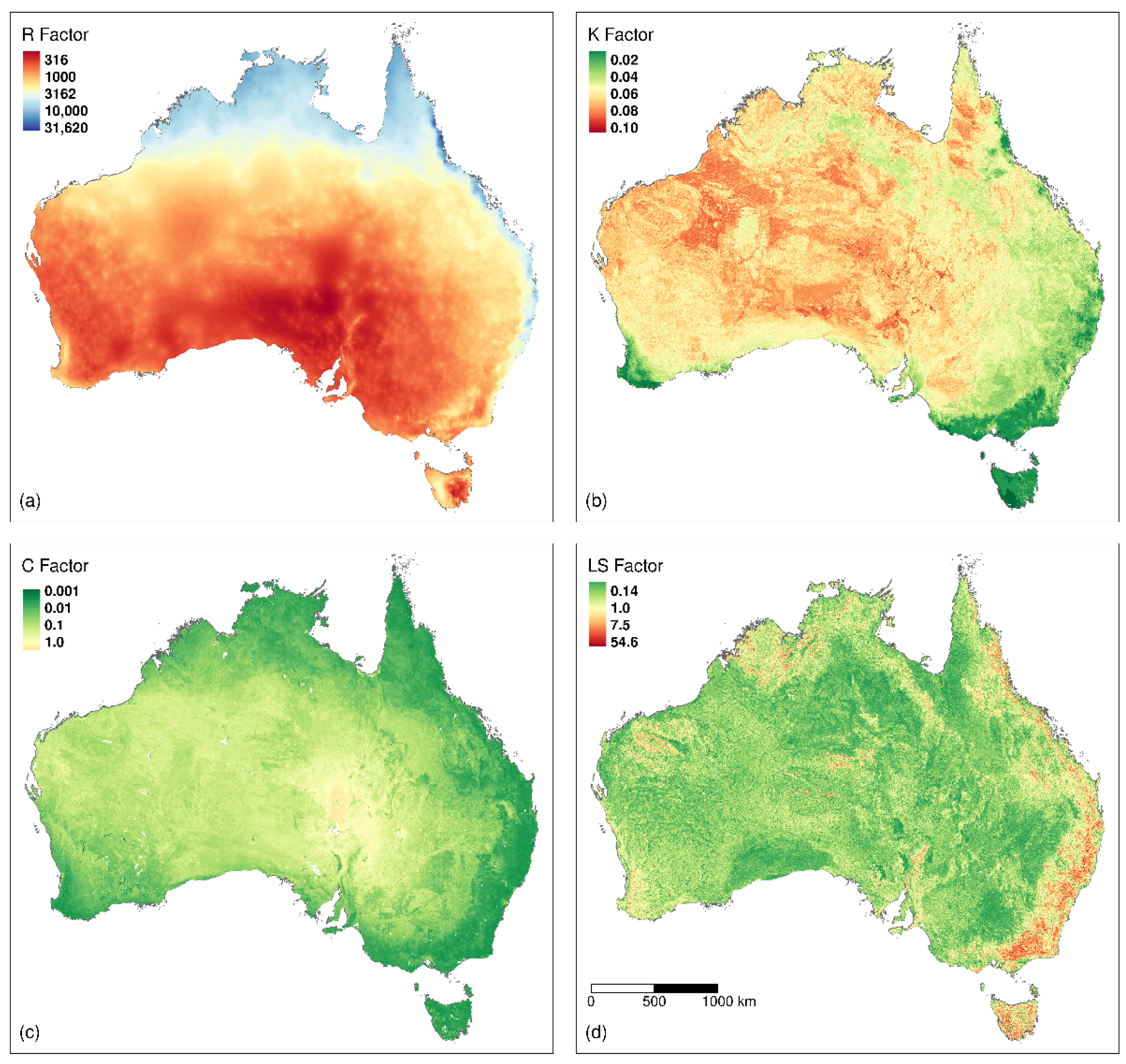
2.2.1. Rainfall Erosivity (R) Factor

Rainfall erosivity is one of the most important input parameters in the RUSLE model to describe water erosion dynamics. We used a regional daily rainfall erosivity model [35] and idealized intensity distributions [36] to estimate the R factor and compared three different rainfall data sources, including Bureau of Meteorology (BoM) gridded daily rainfall and satellite data (TRMM and GPM). The multiple data sources provide means for cross comparison and validation.
E I j = α [ 1 + η c o s ( 2 π f j ω ) ] d = 1 N R d β
Ε = r = 1 N e r · Δ V · I
e r = 0.29 [ 1 0.72 e 0.05 I ]
where EI is the rainfall energy multiplied by the peak rainfall intensity in a certain period j; N is the number of rainy days in the month [37]; and α, β, η, and ω are empirical coefficients used to describe the seasonal (monthly) and locational variations in NSW [35]. In this study, E was computed from rainfall in Equation (3). e r (MJ ha−1 mm−1) denotes the unit kinetic energy in Equation (4).

2.2.2. Cover-Management (C) Factor

The cover and management (C) factor was derived from the most recent (version 3.1.0) and validated fractional vegetation cover (FVC) products, including both photosynthetic vegetation (PV) and non-photosynthetic vegetation (NPV), or the total groundcover (GC) [33]. The monthly FVC time series are available for the entire Australia continent at a spatial resolution of 500 m, from January 2001 to present. The monthly time series of the C factor across Australia were estimated following the method described in [38]:
C j = e ( 0.799 7.74 × G C j + 0.0449 × G C j 2 )
where Cj = RUSLE cover and management factor in month j (1–12) and GCj = groundcover (0–1) in month j (1–12). Ancillary data (e.g., NDVI) and GIS mask layers for water bodies, snow cover, rocky surfaces, cropping, and urban areas were applied to re-adjust the C-factor values and fill in the data gaps [38]. The C factor was resampled to a 90 m resolution to match with the resolutions of the other RUSLE factors. We first used the FVC considering both PV and NPV rather than the traditional green vegetation indices (e.g., NDVI) to estimate the C factor and consequently the hillslope erosion hazard across Australia. It has been demonstrated that the FVC can better reflect the vegetation composition than NDVI [27,33,38].

2.2.3. Slope-Steepness (LS) Factor

The slope-length and steepness (LS) factor (unitless) was calculated from a hydrologically corrected digital elevation model (DEM-H), based on comprehensive algorithms and considering cumulative overland flow length, as described by Yang [39]:
L S = L × S
L = ( λ / 22.13 ) m
m = β / ( 1 + β )
β = ( sin θ 0.0896 ) / [ 3 ( sin θ ) 0.8 + 0.56 ]
S = 10.8 sin θ + 0.03   for   p   <   9 %
S = 16.8 sin θ 0.50   for   p     9 %
where L is the length sub-factor; S is the slope sub-factor; l is the horizontal slope length (m) calculated based on cumulative slope-length at a maximum downhill slope angle; β is a factor that varies with the slope gradient; m is a variable exponent according to β ; θ is the slope steepness angle; and p is the terrain percentage slope (%).
The 30-m DEM-H was used for the LS factor calculation based on Australia Natural Resource Management (NRM) regions, which were then merged to form a seamless LS-factor digital map and resampled to the same resolution (~90 m) as other Australia-wide datasets. Automated scripts were developed and implemented in a Geographic Information System (GIS) for the LS calculation. This represents the LS factor map with the highest spatial resolution in Australia so far.

2.2.4. Soil Erodibility (K) Factor

The soil erodibility factor (RUSLE-K) was estimated based on the RUSLE:
K = [ 2.1 M 1.14 ( 10 4 ) ( 12 O M ) + 3.25 ( 2 S S ) + 2.5 ( P P 3 ) ] / 100 0.1317
where OM is percent soil organic matter (=soil organic carbon × 1.72); SS is the soil structure class; PP is the soil profile permeability class; M is the particle size parameter, which defines the relationship between percentages of silt, very fine sand (VFS), and clay content:
M = (Silt + VFS) (100 − Clay)
where Silt is % silt content (0.002–0.05 mm); VFS is % very fine sand content (0.05–0.1 mm); and Clay is % clay content (<0.002 mm) based on the USDA soil classification. The soil texture and organic matter data were from SLGA with a spatial resolution of 90 m. Soil structure and permeability data were derived from the saturated hydraulic conductivity and grade of pedality attributes of the Australian Soil Resource Information System (ASRIS) [40]. The K factor map has a spatial resolution of 90 m, which matches with the slope-steepness (LS) factor.

2.3. Estimates of Wind Erosion by the Revised Wind Erosion Equation (RWEQ)

The RWEQ model includes a weather factor (WF, kg m−1), erodibility factor (EF, dimensionless), soil crust factor (SCF, dimensionless), roughness (K, dimensionless), and vegetation factor (C, dimensionless). The horizontal sediment flux (Q in kg m−1) and vertical sediment flux ( S L ) are estimated with the following equations:
Q = Q m a x ( 1 e ( Z / S ) 2 )
S L = 2 · Z S 2 Q m a x · e ( Z / S ) 2  
where Q m a x is the maximum transport capacity (in kg m−1); Z is the calculated distance of downwind wind (m); and S is the critical field length (m).
Q m a x = 109.8 [ W F · E F · S C F · K · C ]
S = 150.71 ( W F · E F · S C F · K · C ) 0.3711
The WF integrates the effects of various meteorological factors on wind erosion. It is calculated as
W F = W f · ρ g · S W f · S D
W f = i = 1 i n U 2 ( U 2 U t ) 2 N d 500
S W f = 1 S W
S D = 1 P
where W f is the wind factor (kg m−1); ρ is air density; g is gravity acceleration; S W f is the soil moisture factor; SD is the snow cover factor; and P is the probability that the snow cover depth is greater than 25.4 mm in the simulation period. U 2 is the wind velocity at 2 m; U t is the wind velocity threshold, generally set as 5 m s−1; and N d the number of days in the simulation period (1 day in this study).
The soil erodibility factor (EF) and soil crust factor (SCF) in the RWEQ are expressed by the aggregation of soil particles (especially clay, silty, and soil organic carbon) as follows:
E F = 29.09 + 0.31 S a + 0.17 S i + 0.33 S a C l 2.59 ( S O C 1.72 ) 0.95 C a C O 3 100
S C F = 1 1 + 0.0066 ( C l ) 2 + 0.021 ( S O C 1.72 ) 2
where Sa is the sand grain proportion; Si is the soil silt proportion; Sa/ C l is the ratio of soil sand grain and clay; C l is clay proportion; SOC is soil organic carbon proportion; and CaCO3 is calcium carbonate proportion.
The calculation of surface roughness factor (K’) is based on random roughness factor ( C r r ) and soil roughness ( K r ). As soil roughness ( K r ) is difficult to estimate, the topographic roughness ( K r ) is used instead of soil roughness. It is calculated as follows:
K = e ( 1.86 k r 2.41 k r 0.934 0.127 C r r )
K r = cos α
where α is the slope in radian. The vegetation cover factor is shown as follows:
C = e 0.0438 F V C
where FVC is fractional vegetation cover (in %).

2.4. DustWatch PM10 Measurements

DustWatch has 39 measurement sites (denoted DWN) in south-east Australia. The Tibooburra DWN used in this study had an 8520 model DustTrak® (USA) from January 2009 to July 2019 and a DRX model DustTrak® from August 2019 to December 2020. DustTrak measures the atmospheric aerosol concentration of PM10, as described in [41]. During our study period, Tibooburra was selected as the monitoring site for the model estimates because it is the dustiest site in NSW. In summary, hourly minute PM10 concentration data were averaged to give the monthly concentration (mg m−3) and then converted to the vertical flux ( F h , mg m−2):
F h = P M 10 U f

3. Results

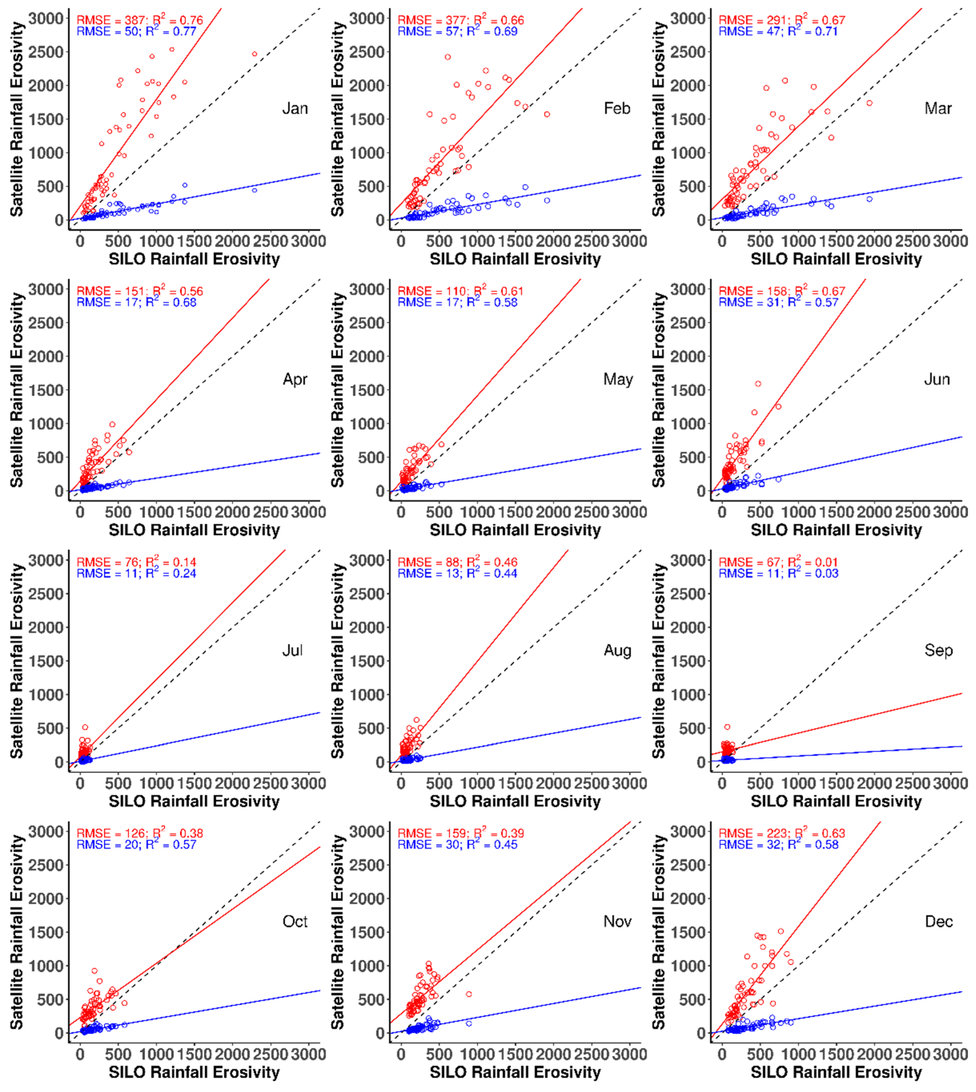
3.1. Assessment and Comparison of Three Satellite Precipitation Products in Rainfall Erosivity

Maps of the water erosion factors in Australia are shown in Figure 1. The annual mean rainfall erosivity for Australia from 2001 to 2020 is show in Figure 1a, revealing high rainfall erosivity in the coastal and tropical areas. The annual average R-factor values calculated from SILO rainfall datasets ranged from 188 MJ mm ha−1 h−1 yr−1 to 19,708 MJ mm ha−1 h−1 yr−1, with a mean of 1786 MJ mm ha−1 h−1 yr−1. TRMM-based R-factor values ranged between 52 MJ mm ha−1 h−1 yr−1 and 3594 MJ mm ha−1 h−1 yr−1, with a mean of 381 MJ mm ha−1 h−1 yr−1, and GPM-based R factor between 187 MJ mm ha−1 h−1 yr−1 to 25,764 MJ mm ha−1 h−1 yr−1, with a mean of 2754 MJ mm ha−1 h−1 yr−1. We found that TRMM tended to underestimate the rainfall erosivity, while GPM overestimated rainfall erosivity. The latter was much closer to the SILO-based calculation but had a larger maximum value.
Figure 1b shows the LS factor layer at 90 m. The LS factor across the Australian continent had a great spatial variation over different landscapes. Higher values were observed in the south-eastern coastline and mountainous regions, while smaller values were mostly found in the lowlands of central Australia. The estimated LS factor values in this study were compared with the reference LS factor values at 300 random points across NSW [39]. In general, the quality of the LS factor values decreased as the DEM resolution became coarser. However, the 90-m LS factor values in this study showed a good correlation with the 30-m LS factor (R2 = 0.91). This is because as the DEM resolution became coarser, the length sub-factor (L) became larger, whilst the slope sub-factor (S) tended to be smoother [42]. Therefore, the LS factor of 90 m in this study matched well with the referenced LS of 30 m under the combined influence of both L and S sub-factors. In Figure 1d, the mean C-factor map (2001–2020) derived from fractional vegetation cover products shows great spatial variation across Australia, reflecting the spatial distribution of vegetation and land cover types. Lower C-factor values (less than or equal to 0.001) coincided spatially with high density vegetation cover along the Great Dividing Range. The higher C-factor values (greater than 0.04) were in the desert and arid areas where vegetation is very limited. The C-factor values also showed strong monthly temporal variations, with more variation in the central semi-arid and arid areas compared to coastal areas with high vegetation cover.
Along the Great Dividing Range in south-eastern Australia, 60 sites were sampled to assess the rainfall erosivity derived from different data sources. Figure 2 shows the linear regression of rainfall erosivity from GPM and TRMM compared to SILO for each month. We found that GPM and TRMM had reasonably good fits in estimating the R factor over south-east Australian rainy seasons (spring and summer) but had poor performance in dry seasons. Comparing the monthly RMSE and R2, TRMM-based R-factor values were generally better than GPM-based R-factor values, with systematic underestimation. When the rainfall erosivity was less than 300 MJ mm ha−1 h−1 m−1, there was little correlation between satellite-based and SILO-based rainfall erosivity.

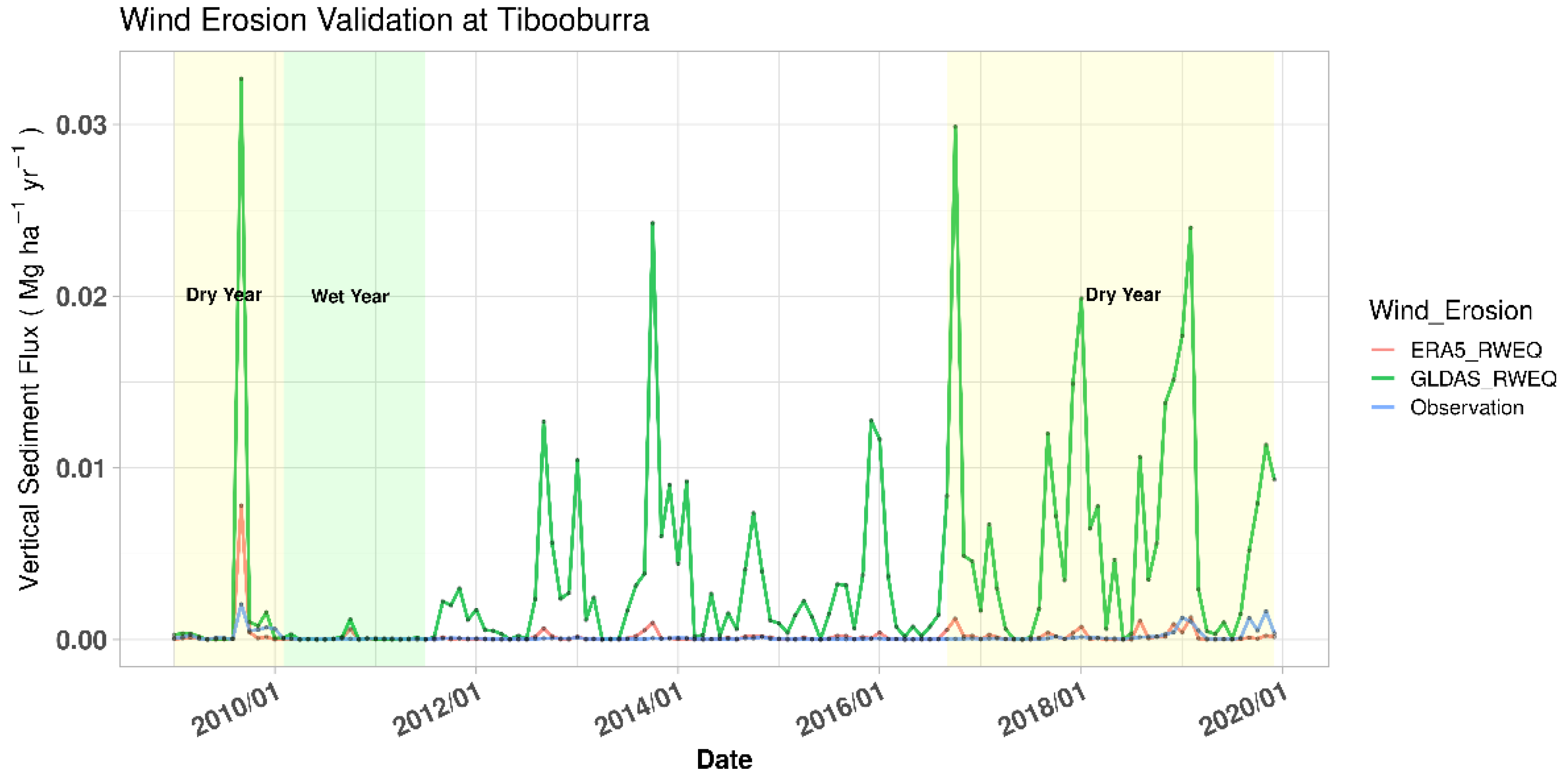
3.2. Validation of Wind Erosion Rates with In Situ Observations

To evaluate the impacts of different data sources on wind erosion results, we compared the model results derived from the GLDAS and ERA5 datasets with the measured wind erosion fluxes at Tibboburra from 2009 to 2019 (Figure 3). Using the GLDAS and ERA5 dataset as model input, Figure 3 shows that the monthly wind erosion fluxes in the RWEQ model. In one financial year (from July to the following June) as an example, the wind erosion generally started to rise in July, reached its highest value in January, and then declined until it reached the lowest values in May. The Australian Bureau of Meteorology (BoM) climate summaries were used to identify wet and dry years. The years from 2010 to 2012 were wet years, while 2001–2009 and 2017–2019 had hot and dry conditions in south-eastern Australia, of which 2009 and 2019 were two particularly dry and dusty years. There was a peak value (~0.002 Mg ha−1 yr−1) in September 2009. Based on our monthly wind erosion results, the extreme value was mainly derived from the wind erosion on 23 September 2009 (a notorious dust storm named Red Dawn occurred, with a maximum wind speed of 12.5 m s−1). We found that the RWEQ model can better capture the extreme dust storm in 2009. In addition, from the beginning of 2010 to later in 2011, the observed flux remained unchanged and lower than the simulated results. As the La Nina in 2010 and 2011 broke the drought, south-eastern Australia entered a wet year. The rainfall increased soil moisture and affected the threshold wind speed of the model. However, the ERA5 datasets-based results did not capture the measured fluxes in 2019, which may have been influenced by the mega-fires in Australia, which were followed by smoke and dust. Overall, using the ERA5 datasets as the model input, the simulated wind erosion fluxes were closer to the measured wind erosion fluxes.

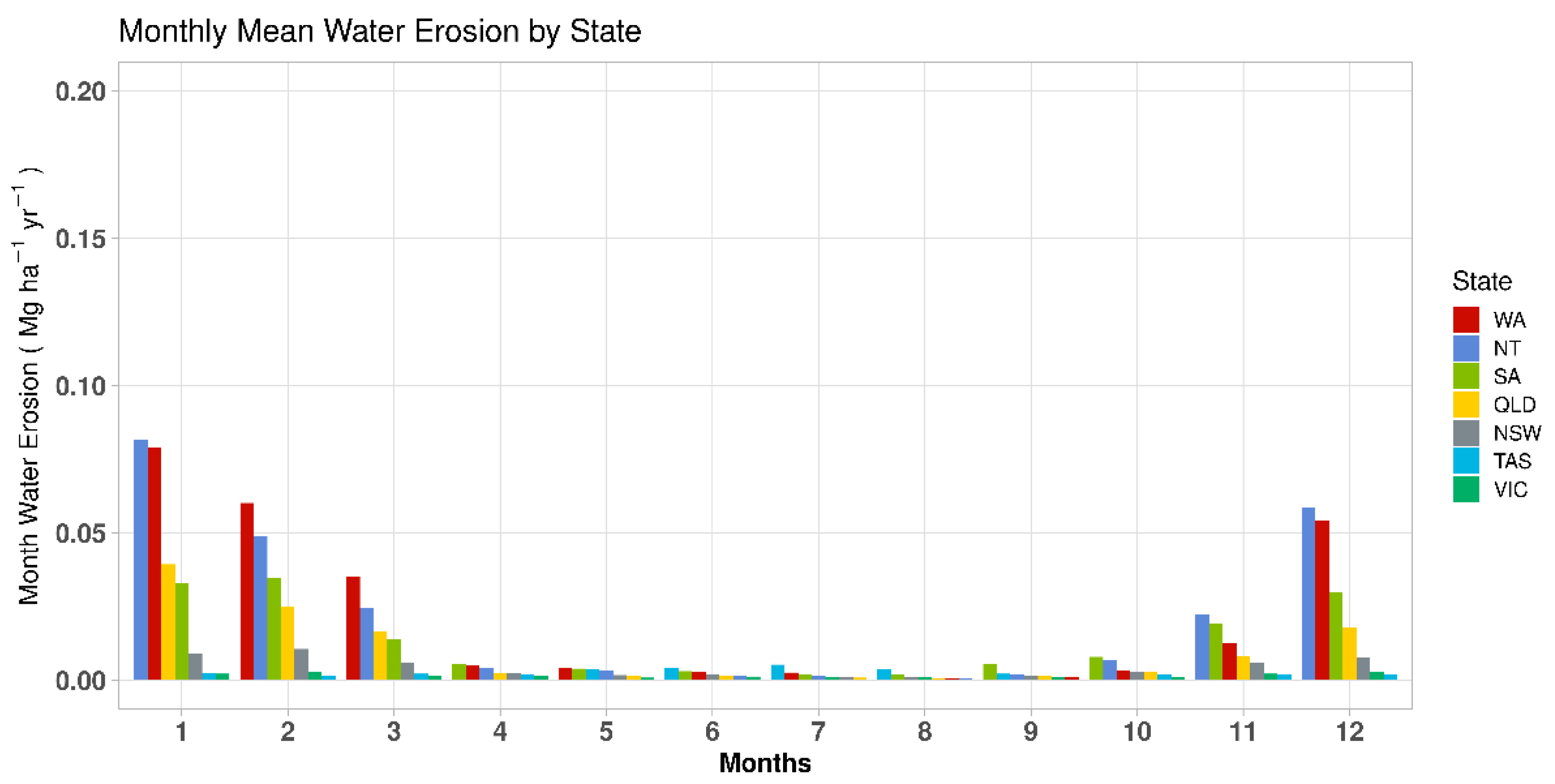
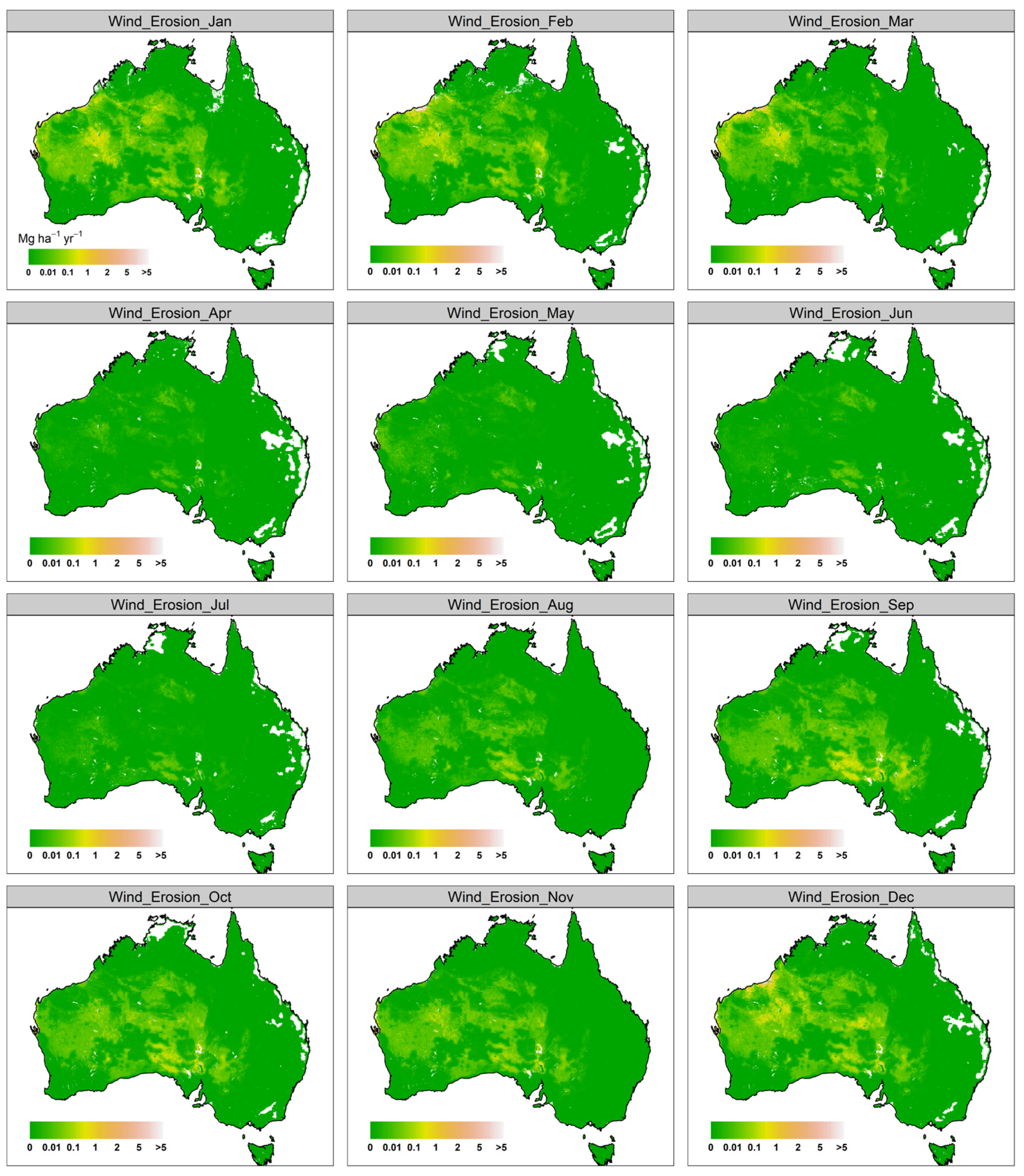
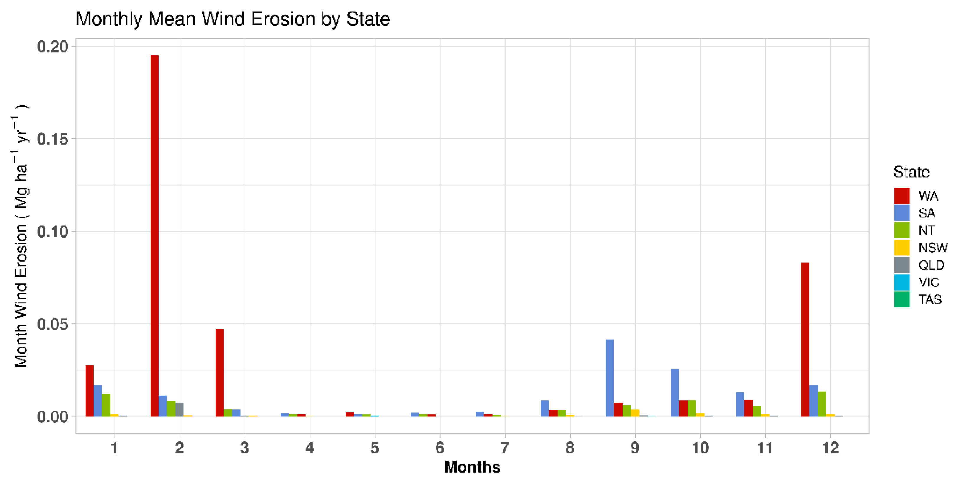
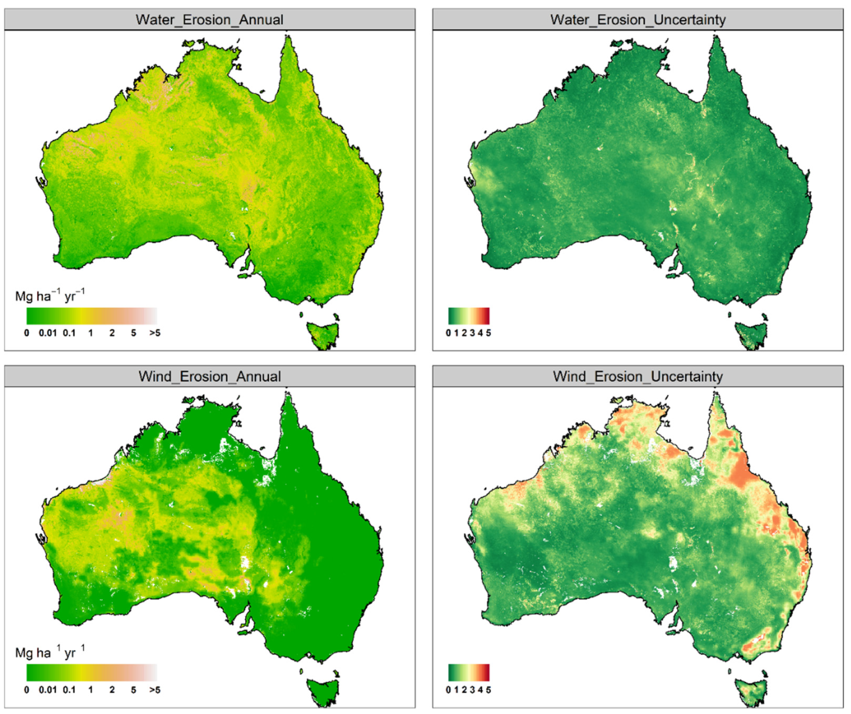
3.3. Monthly and Annually Wind–Water Erosion Maps

We produced the water and wind erosion monthly time-series maps for the period 2001–2020 across Australia. Spatially, the water erosion process across the continent was mainly concentrated in the Great Dividing Range along eastern coastal Australia, Flinders Range in South Australia (SA), Lake Eyre in central Australia, Hamersley Range in Western Australia (WA), Barkly tableland and Arnhem Land in the North Territory (NT), and western coastal Tasmania (TAS) (Figure 4). Moreover, the range of monthly water erosion varied by seasons across Australia. Over summer, high water erosivity was apparent across most of Australia. The summer water erosivity was more evident in northern and south-eastern coastal regions, while water erosivity in winter was relatively weaker because of the reduced rainfall intensity. The most obvious winter water erosivity was observed in the Alpine regions of Victoria and western coastal Tasmania. Figure 5 further demonstrates that northern Australia has the highest water erosion rates in Australia. The top three states in terms of water erosion rate include Western Australian (WA), Queensland (QLD), and NT. Through the year, the highest month of water erosion was January and the lowest was August. Taking WA as an example, water erosion in summer accounted for 74% of total annual erosion, water erosion in spring and winter accounted for 7% and 3%, respectively, and autumn accounted for 16%. The change in the intra-annual trend of water erosion in other states was almost the same as that of WA, except for Tasmania (in the far south of the continent) where it was highest in winter and lowest in summer.
The RWEQ outputs are shown in Figure 6. This shows that the regions with the highest levels of wind erosion match with large dust sources such as the Great Victoria Desert and the Lake Eyre basin. Figure 7 shows that the monthly wind erosion outputs from the RWEQ model exhibit great seasonal differences. This is because the fractional vegetation cover used in the RWEQ model shows greater variation among different landscapes. Furthermore, we also found that wind erosion in SA was greater than in WA from August to November.
Maps of the RUSLE and RWEQ estimated erosion and uncertainty are shown in Figure 8. The uncertainty calculation method used is the range of the 95% confidence intervals over the predicted annual average soil loss. We note that the largest water erosion rates existed around the Kimberley Plateau in northern Australia, Canning Basin in Western Australia, Simpson Desert in central Australia, the coastal wet tropics in Western Australia, and on the south-east slopes in New South Wales and Victoria. Compared to the agricultural areas, the rangeland areas of inland Australia experienced relatively larger water erosion loss, and these larger uncertainties might be due to the rainfall erosivity estimates for dryland areas. On the other hand, wind erosion rates were relatively higher in the rangeland areas where the vegetation cover is sparse, while the uncertainty of wind erosion was notably different between inland regions and coastal regions, as larger uncertainty values are found in the latter.

4. Discussion

The patterns of water and wind erosion are complex due to the combination of several factors, including weather factors (the key driving force), vegetation cover (the key resistance), soil physical properties (determining soil erodibility or resistance to erosion), land cover types (influencing soil surface roughness and soil particles), and the development of wind profiles. In this study, we estimated both water and wind erosion using the RUSLE and RWEQ models. The RUSLE and RWEQ models were implemented in the GEE environment to enable spatio-temporal soil erosion modelling at any scale. The application of water and wind models across Australia provided time-series datasets in states and territories like WA and NT, where very high soil loss rates cannot be neglected. In Australia, water erosion is higher in the summer months, especially in February when there is more intense rainfall [9]. Wind erosion is normally higher in spring and summer when there is less groundcover and more dry weather [8,10].
As compared to the RUSLE sub-factors in the CSIRO data portal, we found that the C factor exhibits significant differences over space. The differences are from the vegetation cover datasets. In our estimates, we used the dynamic fractional vegetation cover as described by Guerschman et al. [33] to estimate the C factor, whereas the C-factor values from Teng et al. [25] are solely based on static land cover classification. The largest C-factor values from Teng et al. [25] cover all the arid and desert areas in central and Western Australia. Our C-factor estimates have the largest values in the Lake Eyre basin of central Australia. Despite the under- and overestimation of the R-factor values by GPM and TRMM, the multi-year R-factor values derived by station-based daily rainfall data at a resolution of 5 km are also better than satellite-based R factor. Lu et al. [43] derived water erosion rates in Australia during the period 1980–2000, with a mean water erosion of 11.77 Mg ha−1 yr−1. The estimate of the area weighted mean water erosion produced by Teng et al. [25] is 0.69 Mg ha−1 yr−1. Our annual mean estimate of erosion in Australia during the 2001 to 2020 period is 0.17 Mg ha−1 yr−1. Compared to Teng et al. [25], our estimate of erosion is smaller and more conservative. The major reason is the use of fractional vegetation cover in our study, which considers both green and non-green vegetation, while the previous studies only considered the green vegetation in erosion modelling. Chappell et al. [8] provided the net erosion distribution of Australia over the period of 1950–1990, and our map shows a similar erosion distribution in central Australia, while other estimates cannot capture the erosion in that area. The average rates of water modelled over Australia in our study are also broadly comparable with rates reported by other studies across the globe [1,2,6,23,29,44]. However, the rates of water erosion from the dry central Australian regions appear to be amongst the highest reported from these international studies.
In the RUSLE model, rainfall erosivity is the most dominant agent, meaning changes in rainfall have a great impact on changes in water erosion trends [44,45]. Generally, Australian rainfall in the past two decades experienced substantial inter-annual variability, with short wet periods (2010–2011, 2020) and longer dry periods (e.g., 2002–2009 and 2012–2019). Liu et al. [46] found that Australian rainfall changes had a trend of short and frequent rainfall events, which meant that most rainfall tended to evaporation rather than increasing soil moisture. It is highly important to improve the accuracy of models to better understand how erosion and post-extreme weather (e.g., storms, bushfires) impact ecosystems. However, the trend of water erosion changes is not always in agreement with rainfall changes. The significant vegetation cover declines resulting from bushfires also contribute to the increase in water erosion. A very strong water erosion peak in 2020 in our study shows that the increase in rainfall intensity and decrease in vegetation cover together were in line with the substantial increase in water erosion at that time. That is because extreme storms contribute to high rainfall erosivity, but, at the same time, quick and short rainfall events are not adequate to support high vegetation cover [37].
Unlike changes in rainfall, the long-term variability and seasonal patterns of near-surface wind speed for the past two decades are still poorly understood. The dry conditions and decrease in soil moisture also have an impact on wind erosion. In this study, we used the RWEQ model to predict wind erosion in Australia. Our estimate of the annual mean of wind erosion across the country is 0.29 Mg ha−1 yr−1. Compared to the RWEQ simulated results from [47], we shared similar wind erosion distribution patterns in the dry rangelands, but our estimates are much smaller. We also attempted to validate the process-based RWEQ model against real-time field observations. For most of the dry periods, the measured fluxes were less than our simulated results but the changing patterns were well matched. This may be the reason that the DWN flux measurements do not adequately represent real wind erosion, for example, fine dust may travel thousands of kilometers or remain in air until it is washed out by rainfall.
The RUSLE model used in this study was supported and calibrated using field monitoring and regional-scale models. Our water erosion study largely relied on the prediction of rainfall erosivity, which had limitations associated with the smaller and frequent rainfall events, characterized by a decreased rainfall intensity and an increased rainfall probability. However, the RWEQ model with original parameters is not well calibrated using local data from site observations collected at a regional scale. Therefore, uncertainties will be introduced when it is applied for monthly estimations because the parameters in the RWEQ vary in spatio-temporal scale. For example, the two dynamic sub-factors of vegetation cover and soil moisture effects in the RWEQ model need to be calibrated locally, as was the case for the local coefficients of vegetation cover effects on wind erosion in the AUSLEM, which were determined by wind tunnel experimentation at a wind speed of 18 m s−1 [48].
Therefore, the emphasis of future studies should be placed on improving accuracy and developing new models of water and wind erosion. In addition, the future increase in the amount of high-resolution remote sensing and big data will lead to improved estimation for vegetation, soil, topography, and other biophysical factors, which will, in turn, improve the estimation of soil erosion and assist in calibrating and validating water and wind erosion models. It is acknowledged that the climate and vegetation cover are two key factors contributing to soil erosion changes. Possible areas of improvement are the use of high-quality fractional vegetation cover, radar-based rainfall erosivity, and soil moisture estimation. For example, we can derive the monthly C factor at a 20 m resolution from Sentinel 2, with gap filling using image blending techniques. As the weather radar data across Australia become increasingly available, we are able to further explore the use of radar-derived rainfall erosivity with advanced machine learning models to simulate water erosion. Better soil moisture data (e.g., AWAP and SMIPS) can also be used to replace the soil moisture data from the global-scale ERA5 dataset. Furthermore, soil loss can be estimated using the strengths of the process-based RUSLE and RWEQ models, while utilizing insights from the physical mechanism of erosion formation and exploiting the predictive capacity of machine learning with remote-sensed big EO data.

5. Conclusions

In this study, we used the best available big EO data from across Australia during the past two decades to derive water and wind erosion datasets and analyze the spatio-temporal variability of soil erosion. We estimated rainfall erosivity across Australia using satellite-based rainfall data and compared the results with the ground-based SILO data, showing consistent spatial patterns. We also found a persistent agreement between our wind erosion model and the measured vertical sediment flux, but with an apparent underestimation of the measured flux. It is notable that the RWEQ model can capture the erosion caused by extreme climate events. In practice, our wind erosion model results demonstrate that the reanalysis data of ERA5 exhibit better performance than GLDAS data. At the monthly scale, water and wind erosion have strong inter-annual seasonality. In the past two decades, the trends of annual water erosion vary among different states, while annual wind erosion has exhibited an increasing trend since 2010. Nevertheless, we believe our study is the first attempt to produce a combined water and wind erosion dataset across Australia, which offers a new perspective for understanding soil erosion and its behavior in relation to climate, land, and soil conditions.

Author Contributions

Conceptualization, X.Y., J.L. and Q.Y.; Methodology, X.Y. and J.L.; Software and validation and formal analysis, M.Z.; Resources, X.Y., J.L., R.A.V.R. and Q.Y.; Writing—original draft preparation, M.Z.; Writing—review and editing, X.Y., R.A.V.R., J.L., J.M.G., Q.Z. and M.Z.; Visualization, M.Z. All authors have read and agreed to the published version of the manuscript.

Funding

This research received no external funding.

Data Availability Statement

Mingxi Zhang, Raphael A. Viscarra Rossel, Qinggaozi Zhu, John Leys, Jonathan M. Gray, Qiang Yu, and Xihua Yang. (2022). Water and Wind Erosion in Australia during the past two decades [Data set]. Zenodo. https://0-doi-org.brum.beds.ac.uk/10.5281/zenodo.7115399.

Acknowledgments

We thank Stephan Heidenreich from the NSW Department of Planning and Environment for assistance with access the Tibooburra DustWatch data.

Conflicts of Interest

The authors declare no conflict of interest.

References

  1. Borrelli, P.; Robinson, D.A.; Fleischer, L.R.; Lugato, E.; Ballabio, C.; Alewell, C.; Meusburger, K.; Modugno, S.; Schutt, B.; Ferro, V.; et al. An assessment of the global impact of 21st century land use change on soil erosion. Nat. Commun. 2017, 8, 2013. [Google Scholar] [CrossRef] [PubMed] [Green Version]
  2. Food and Agriculture Organization. Status of the World’s Soil Resources (SWSR)–Main Report; Food and Agriculture Organization of the United Nations and Intergovernmental Technical Panel on Soils: Rome, Italy, 2015. [Google Scholar]
  3. Telles, T.S.; Dechen, S.C.F.; de Souza, L.G.A.; Guimarães, M.D.F. Valuation and assessment of soil erosion costs. Sci. Agric. 2013, 70, 209–216. [Google Scholar] [CrossRef]
  4. Faeth, P. Building the Case for Sustainable Agriculture: Policy Lessons from India, Chile, and Chile, and the Philippines. Environ. Sci. Policy Sustain. Dev. 1994, 36, 16–39. [Google Scholar] [CrossRef]
  5. Chappell, A.; Webb, N.P.; Leys, J.F.; Waters, C.M.; Orgill, S.; Eyres, M.J. Minimising soil organic carbon erosion by wind is critical for land degradation neutrality. Environ. Sci. Policy 2019, 93, 43–52. [Google Scholar] [CrossRef]
  6. Middleton, N. Variability and Trends in Dust Storm Frequency on Decadal Timescales: Climatic Drivers and Human Impacts. Geosciences 2019, 9, 261. [Google Scholar] [CrossRef] [Green Version]
  7. Bui, E.; Hancock, G.; Chappell, A.; Gregory, L. Evaluation of Tolerable Erosion Rates and Time to Critical Topsoil Loss in Australia; CSIRO Land and Water: Canberra, Australia, 2010; p. 87. [Google Scholar]
  8. Chappell, A.; Hancock, G.; Rossel, R.A.V.; Loughran, R. Spatial uncertainty of the137Cs reference inventory for Australian soil. J. Geophys. Res. 2011, 116, F04014. [Google Scholar] [CrossRef]
  9. Yang, X.; Zhang, M.; Oliveira, L.; Ollivier, Q.R.; Faulkner, S.; Roff, A. Rapid Assessment of Hillslope Erosion Risk after the 2019–2020 Wildfires and Storm Events in Sydney Drinking Water Catchment. Remote Sens. 2020, 12, 3805. [Google Scholar] [CrossRef]
  10. Leys, J.F.; Heidenreich, S.K.; Strong, C.L.; McTainsh, G.H.; Quigley, S. PM10 concentrations and mass transport during “Red Dawn”–Sydney 23 September 2009. Aeolian Res. 2011, 3, 327–342. [Google Scholar] [CrossRef] [Green Version]
  11. Karydas, C.G.; Panagos, P.; Gitas, I.Z. A classification of water erosion models according to their geospatial characteristics. Int. J. Digit. Earth 2014, 7, 229–250. [Google Scholar] [CrossRef]
  12. Meyer, H.; Reudenbach, C.; Hengl, T.; Katurji, M.; Nauss, T. Improving performance of spatio-temporal machine learning models using forward feature selection and target-oriented validation. Environ. Model. Softw. 2018, 101, 1–9. [Google Scholar] [CrossRef]
  13. Laflen, J.M.; Elliot, W.; Flanagan, D.; Meyer, C.; Nearing, M. WEPP-predicting water erosion using a process-based model. J. Soil Water Conserv. 1997, 52, 96–102. [Google Scholar]
  14. Yu, B.; Rose, C. Application of a physically based soil erosion model, GUEST, in the absence of data on runoff rates I. Theory and methodology. Soil Res. 1999, 37, 1–12. [Google Scholar] [CrossRef]
  15. Rahmati, O.; Tahmasebipour, N.; Haghizadeh, A.; Pourghasemi, H.R.; Feizizadeh, B. Evaluation of different machine learning models for predicting and mapping the susceptibility of gully erosion. Geomorphology 2017, 298, 118–137. [Google Scholar] [CrossRef]
  16. Fryrear, D.; Bilbro, J.; Saleh, A.; Schomberg, H.; Stout, J.; Zobeck, T. RWEQ: Improved wind erosion technology. The wind erosion prediction system and its use in conservation planning. J. Soil Water Conserv. 2000, 55, 183–189. [Google Scholar]
  17. Chappell, A.; Webb, N.P. Using albedo to reform wind erosion modelling, mapping and monitoring. Aeolian Res. 2016, 23, 63–78. [Google Scholar] [CrossRef] [Green Version]
  18. Tatarko, J.; Wagner, L.; Fox, F. The wind erosion prediction system and its use in conservation planning. Wind. Eros. Predict. Syst. Its Use Conserv. Plan. 2019, 8, 71–101. [Google Scholar]
  19. Kok, J.F.; Mahowald, N.M.; Fratini, G.; Gillies, J.A.; Ishizuka, M.; Leys, J.F.; Mikami, M.; Park, M.S.; Park, S.U.; van Pelt, R.S.; et al. An improved dust emission model–Part 1: Model description and comparison against measurements. Atmos. Chem. Phys. 2014, 14, 13023–13041. [Google Scholar] [CrossRef] [Green Version]
  20. Chappell, A.; Webb, N.P.; Guerschman, J.P.; Thomas, D.T.; Mata, G.; Handcock, R.N.; Leys, J.F.; Butler, H.J. Improving ground cover monitoring for wind erosion assessment using MODIS BRDF parameters. Remote Sens. Environ. 2018, 204, 756–768. [Google Scholar] [CrossRef]
  21. Borrelli, P.; Robinson, D.A.; Panagos, P.; Lugato, E.; Yang, J.E.; Alewell, C.; Wuepper, D.; Montanarella, L.; Ballabio, C. Land use and climate change impacts on global soil erosion by water (2015–2070). Proc. Natl. Acad. Sci. USA 2020, 117, 21994–22001. [Google Scholar] [CrossRef] [PubMed]
  22. Youssef, F.; Visser, S.; Karssenberg, D.; Bruggeman, A.; Erpul, G. Calibration of RWEQ in a patchy landscape; a first step towards a regional scale wind erosion model. Aeolian Res. 2012, 3, 467–476. [Google Scholar] [CrossRef] [Green Version]
  23. Borrelli, P.; Lugato, E.; Montanarella, L.; Panagos, P. A New Assessment of Soil Loss Due to Wind Erosion in European Agricultural Soils Using a Quantitative Spatially Distributed Modelling Approach. Land Degrad. Dev. 2016, 28, 335–344. [Google Scholar] [CrossRef] [Green Version]
  24. Pi, H.; Sharratt, B.; Feng, G.; Lei, J. Evaluation of two empirical wind erosion models in arid and semi-arid regions of China and the USA. Environ. Model. Softw. 2017, 91, 28–46. [Google Scholar] [CrossRef] [Green Version]
  25. Teng, H.; Rossel, R.V.; Shi, Z.; Behrens, T.; Chappell, A.; Bui, E. Assimilating satellite imagery and visible–near infrared spectroscopy to model and map soil loss by water erosion in Australia. Environ. Model. Softw. 2016, 77, 156–167. [Google Scholar] [CrossRef]
  26. McKenzie, N.; Hairsine, P.; Gregory, L.; Austin, J.; Baldock, J.; Webb, M.; Mewett, J.; Cresswell, H.; Welti, N.; Thomas, M. Priorities for Improving Soil Condition across Australia's Agricultural Landscapes; CSIRO Agriculture and Food: Canberra, Australia, 2017. [Google Scholar]
  27. Yang, X. State and trends of hillslope erosion across New South Wales, Australia. CATENA 2020, 186, 104361. [Google Scholar] [CrossRef]
  28. Atiqul Islam, M.; Yu, B.; Cartwright, N. Assessment and comparison of five satellite precipitation products in Australia. J. Hydrol. 2020, 590, 125474. [Google Scholar] [CrossRef]
  29. Jiang, C.; Zhang, H.; Zhang, Z.; Wang, D. Model-based assessment soil loss by wind and water erosion in China's Loess Plateau: Dynamic change, conservation effectiveness, and strategies for sustainable restoration. Glob. Planet. Chang. 2019, 172, 396–413. [Google Scholar] [CrossRef]
  30. Gorelick, N.; Hancher, M.; Dixon, M.; Ilyushchenko, S.; Thau, D.; Moore, R. Google Earth Engine: Planetary-scale geospatial analysis for everyone. Remote Sens. Environ. 2017, 202, 18–27. [Google Scholar] [CrossRef]
  31. Rodell, M.; Houser, P.; Jambor, U.; Gottschalck, J.; Mitchell, K.; Meng, C.-J.; Arsenault, K.; Cosgrove, B.; Radakovich, J.; Bosilovich, M. The global land data assimilation system. Bull. Am. Meteorol. Soc. 2004, 85, 381–394. [Google Scholar] [CrossRef] [Green Version]
  32. Hersbach, H.; Bell, B.; Berrisford, P.; Hirahara, S.; Horányi, A.; Muñoz-Sabater, J.; Nicolas, J.; Peubey, C.; Radu, R.; Schepers, D.; et al. The ERA5 global reanalysis. Quarterly J. R. Meteorol. Soc. 2020, 146, 1999–2049. [Google Scholar] [CrossRef]
  33. Guerschman, J.P.; Hill, M.J. Calibration and validation of the Australian fractional cover product for MODIS collection 6. Remote Sens. Lett. 2018, 9, 696–705. [Google Scholar] [CrossRef]
  34. Viscarra Rossel, R.A.; Chen, C.; Grundy, M.J.; Searle, R.; Clifford, D.; Campbell, P.H. The Australian three-dimensional soil grid: Australia’s contribution to the GlobalSoilMap project. Soil Res. 2015, 53, 845–864. [Google Scholar] [CrossRef] [Green Version]
  35. Yang, X.; Yu, B. Modelling and mapping rainfall erosivity in New South Wales, Australia. Soil Res. 2015, 53, 178–189. [Google Scholar] [CrossRef]
  36. Brown, L.; Foster, G. Storm erosivity using idealized intensity distributions. Trans. ASAE 1987, 30, 379–0386. [Google Scholar] [CrossRef]
  37. Zhu, Q.; Yang, X.; Yu, B.; Tulau, M.; McInnes-Clarke, S.; Nolan, R.H.; Du, Z.; Yu, Q. Estimation of event-based rainfall erosivity from radar after wildfire. Land Degrad. Dev. 2019, 30, 33–48. [Google Scholar] [CrossRef] [Green Version]
  38. Yang, X. Deriving RUSLE cover factor from time-series fractional vegetation cover for hillslope erosion modelling in New South Wales. Soil Res. 2014, 52, 253–261. [Google Scholar] [CrossRef]
  39. Yang, X. Digital mapping of RUSLE slope length and steepness factor across New South Wales, Australia. Soil Res. 2015, 53, 216–225. [Google Scholar] [CrossRef]
  40. McKenzie, N.; Jacquier, D.; Ashton, L.; Cresswell, H. Estimation of Soil Properties Using the Atlas of Australian Soils, in CSIRO Land Water Technical Report; CSIRO Publishing: Clayton, Australia, 2000; pp. 1–12. [Google Scholar]
  41. Leys, J.; Strong, C.; Heidenreich, S.; Koen, T. Where She Blows! A Ten Year Dust Climatology of Western New South Wales Australia. Geosciences 2018, 8, 232. [Google Scholar] [CrossRef] [Green Version]
  42. Shan, L.; Yang, X.; Zhu, Q. Effects of DEM resolutions on LS and hillslope erosion estimation in a burnt landscape. Soil Res. 2019, 57, 797. [Google Scholar] [CrossRef]
  43. Lu, H.; Prosser, I.P.; Moran, C.J.; Gallant, J.C.; Priestley, G.; Stevenson, J.G. Predicting sheetwash and rill erosion over the Australian continent. Soil Res. 2003, 41, 1037–1062. [Google Scholar] [CrossRef]
  44. Sun, W.; Shao, Q.; Liu, J.; Zhai, J. Assessing the effects of land use and topography on soil erosion on the Loess Plateau in China. CATENA 2014, 121, 151–163. [Google Scholar] [CrossRef]
  45. Du, H.-q.; Xue, X.; Wang, T. Mapping the risk of water erosion in the watershed of the Ningxia-Inner Mongolia reach of the Yellow River, China. J. Mt. Sci. 2015, 12, 70–84. [Google Scholar] [CrossRef]
  46. Liu, D.L.; Teng, J.; Ji, F.; Anwar, M.R.; Feng, P.; Wang, B.; Li, L.; Waters, C. Characterizing spatiotemporal rainfall changes in 1960–2019 for continental Australia. Int. J. Climatol. 2020, 41, 2420–2444. [Google Scholar] [CrossRef]
  47. Yang, G.; Sun, R.; Jing, Y.; Xiong, M.; Li, J.; Chen, L. Global assessment of wind erosion based on a spatially distributed RWEQ model. Prog. Phys. Geogr. Earth Environ. 2021, 46, 28–42. [Google Scholar] [CrossRef]
  48. Webb, N.P.; McGowan, H.A.; Phinn, S.R.; Leys, J.F.; McTainsh, G.H. A model to predict land susceptibility to wind erosion in western Queensland, Australia. Environ. Model. Softw. 2009, 24, 214–227. [Google Scholar] [CrossRef]
Figure 1. Maps of the RUSLE factors: (a) rainfall erosivity factor; (b) soil erodibility factor; (c) annual average cover management factor from 2001–2020; (d) slope length and steepness factor.
Remotesensing 14 05437 g001
Figure 2. Comparison between the R-factor values derived from SILO, GPM, and TRMM for 12 months along the Great Dividing Range in south-eastern Australia.
Remotesensing 14 05437 g002
Figure 3. Monthly wind erosion values from the ERA5_RWEQ model, the GLDAS_RWEQ model, and the observations at the Tibooburra site compared for the period 2009 to 2019.
Remotesensing 14 05437 g003
Figure 4. Monthly water erosion based on SILO in 2001–2020.
Remotesensing 14 05437 g004
Figure 5. Bar chart of monthly water erosion by state in 2001–2020.
Remotesensing 14 05437 g005
Figure 6. Monthly wind erosion based on the RWEQ model in 2001–2020.
Remotesensing 14 05437 g006
Figure 7. Bar chart of monthly wind erosion by state based on the RWEQ in 2001–2020.
Remotesensing 14 05437 g007
Figure 8. Annual average water and wind erosion and uncertainty based on the RUSLE and RWEQ in 2001–2020.
Remotesensing 14 05437 g008
Table 1. Datasets used in this study.
DatasetDescriptionSpatial ResolutionTime PeriodData PortalModel
SILOScientific Information for LandOwner’s climate database5 km1920–2020, dailyGEERUSLE
DEMAustralian SRTM Hydrologically Enforced Digital Elevation Model30 m2010GEERUSLE/RWEQ
FVCFractional Vegetation Cover500 m2000–2020, dailyCSIRORUSLE/RWEQ
GPMGlobal Precipitation Measurement10 km3 hGEERUSLE
TRMMThe Tropical Rainfall Measuring Mission25 km3 hGEERUSLE
SLGASoil and Landscape Grid of Australia90 m-GEERUSLE/RWEQ
GLDASGlobal Land Data Assimilation System25 km3 hGEERWEQ
ERA5 ECMWF Reanalysis 5 (ERA5) atmospheric reanalysis25 km3 hGEERWEQ
Publisher’s Note: MDPI stays neutral with regard to jurisdictional claims in published maps and institutional affiliations.

