

Change Alignment-Based Image Transformation for Unsupervised Heterogeneous Change Detection

College of Electronic Science, National University of Defense Technology, Changsha 410073, China
*
Author to whom correspondence should be addressed.
Remote Sens. 2022, 14(21), 5622; https://0-doi-org.brum.beds.ac.uk/10.3390/rs14215622
Submission received: 12 September 2022
/
Revised: 17 October 2022
/
Accepted: 3 November 2022
/
Published: 7 November 2022
(This article belongs to the Special Issue Image Change Detection Research in Remote Sensing)
Abstract
:Change detection (CD) with heterogeneous images is currently attracting extensive attention in remote sensing. In order to make heterogeneous images comparable, the image transformation methods transform one image into the domain of another image, which can simultaneously obtain a forward difference map (FDM) and backward difference map (BDM). However, previous methods only fuse the FDM and BDM in the post-processing stage, which cannot fundamentally improve the performance of CD. In this paper, a change alignment-based change detection (CACD) framework for unsupervised heterogeneous CD is proposed to deeply utilize the complementary information of the FDM and BDM in the image transformation process, which enhances the effect of domain transformation, thus improving CD performance. To reduce the dependence of the transformation network on labeled samples, we propose a graph structure-based strategy of generating prior masks to guide the network, which can reduce the influence of changing regions on the transformation network in an unsupervised way. More importantly, based on the fact that the FDM and BDM are representing the same change event, we perform change alignment during the image transformation, which can enhance the image transformation effect and enable FDM and BDM to effectively indicate the real change region. Comparative experiments are conducted with six state-of-the-art methods on five heterogeneous CD datasets, showing that the proposed CACD achieves the best performance with an average overall accuracy (OA) of on different datasets and at least improvement in the kappa coefficient.
1. Introduction
1.1. Background
The change detection (CD) technique of remote sensing images aims to detect changes in ground objects between two or more images acquired at different times in the same geographical area [1]. With the continuous improvement of spatial and temporal resolution of remote sensing images, CD technology is continuously applied and promoted in various fields, such as land cover, buildings, ecosystem services and natural disaster assessment [2]. (1) Land cover. Land cover change detection using remote sensing images is an important application of Earth observation data because it provides insight into environmental health, global warming, and urban management. Lv et al. [3] review the problem of land cover change detection using remote sensing images in terms of algorithms, applications, etc., to promote a comprehensive understanding of land cover research with high-resolution images. (2) Buildings are one of the most dynamic man-made structures. Building change detection is important for urban development monitoring (e.g., building demolition and construction) and disaster management (e.g., building damage caused by natural disasters). Bai et al. [4] propose an end-to-end edge-guided recursive convolutional neural network building change detection method. The main idea is to combine the distinguishing information and edge structure prior information in a framework to improve the change detection results, especially to generate more accurate building boundaries. (3) Ecosystem services link ecosystems to human well-being by considering nature as a resource that provides a range of services (e.g., local climate regulation and water purification) [5]. (4) CD is an urgent issue in natural disaster assessment. Fast and effective identification of the affected area can better carry out rescue and damage assessment. Brunner et al. [6] use optical image and SAR image to detect the affected area after the earthquake.
Most of the current CD techniques [7,8,9] are based on homogeneous data, which are acquired by the same sensors, such as optical sensor or synthetic aperture radar (SAR) sensor. Unfortunately, homogeneous images are not available the first time for some reason, so we started to focus our attention on heterogeneous CD, i.e., using images from different sensors. The CD by heterogeneous images has two advantages: (1) It improves the temporal resolution by inserting heterogeneous image to satisfy the requirements of specific applications with strict constraints [10]. (2) Since it chooses the first available image to detect the change instead of waiting for a homogeneous image that can be directly compared, it reduces the response time for CD, which has significant application needs in the rescue and evaluation of natural disasters such as floods and earthquakes [11,12]. Despite the urgent demand for heterogeneous CD and its wide application prospect, the research on it is in its infancy. There are still many unsolved problems and research difficulties. The variability between heterogeneous remote sensing images is considerable, and the images acquired by different sensors cannot be compared directly and need to be converted to the same space for this purpose. This involves several difficulties as follows. (1) Assimilation mapping is difficult. Heterogenous remote sensing images have different imaging mechanisms, provide different descriptions of the same feature, and exhibit different characteristics. Therefore, mapping heterogeneous images into the same space is a difficult problem. (2) The effect of image noise. The inherent noise in the image (such as coherent speckle noise in SAR images) can affect the accuracy of image classification and reduce the quality of difference maps, and thus increase false and missed detections, resulting in the degradation of CD performance. (3) Impact of high resolution. The task of heterogeneous CD becomes more complex under high-resolution conditions. It also brings the increase of image size, which makes the size of the solution problem the scale of the solution problem becomes larger, which puts higher requirements on the computational complexity of the algorithm.
1.2. Related Work
The challenge of heterogeneous CD is that the images before and after the moment are in different domains because different sensors have different imaging mechanisms, it cannot detect changes with simple arithmetic operations as homogeneous images, such as image difference [13] (usually for optical images) and image ratio [14]/log-ratio [15] (usually for SAR images).
Many methods [16,17,18] have been developed to solve this challenge by transforming the images into the same space, where the images can be compared directly. These methods can be divided into the following three categories.
(1) Classification space-based methods. In this type of method, heterogeneous images are transformed into a common image category space. They detect changes by comparing the classification results of multi-temporal images. Among them, the most widely used is the post-classification comparison algorithm (PCC) [19]. The accuracy of this method depends heavily on the performance of image classification, and PCC is also affected by error propagation or accumulation. To address this challenge, Wan et al. [20] recently proposed a change detection method based on multitemporal segmentation and composite classification (MS-CC). However, as demonstrated in the literature, the method is strongly influenced by image segmentation, especially for SAR images, where accurate segmentation is difficult. The advantages of such methods are that they are intuitive and easy to implement, and the type of methods is able to show what type of changes before and after moments are better able to meet the needs. However, they generally have the following disadvantages: the CD accuracy is limited by the accuracy and precision of the classification, and there is also the risk of accumulation of classification errors.
(2) Feature space-based methods. This category of methods [21,22,23,24] is constructed by transforming heterogeneous images into the same feature space, which is constructed manually or learned by deep network. The motivation for manually constructing features is to find shared features and feature similarities of heterogeneous images. Sun et al. [25] construct graph structure features for each patch based on non-local patch similarity, which measures the degree of change by measuring the graph structure similarity between two images before and after. Sun et al. [26] combine difference maps generation and the computation of binary change maps for iteration to generate more robust graphs. When the geographic type is complicated, the quality of the change map will be affected by the difficulty of constructing a suitable feature space for mapping. As for the methods of learning features through a deep network, which are used to extract high-dimensional features for CD, Zhao et al. [27] propose a symmetric convolutional coupled network (SCCN) that maps discriminative features of heterogeneous images to common feature space. Lv et al. [28] embed the multiscale convolutional module into the U-Net backbone network to extract features for covering ground targets of different sizes and shapes. Chen et al. [29] propose a self-supervised method to extract good feature representation from multi-view images by contrast learning, which can correctly align features learned from images acquired at different times. Although network-based learning methods are superior in detection accuracy, these methods suffer from two major drawbacks: the time-consuming training process and the construction of training sets, which require manual labeling of samples in a supervised network [24,30] or a complex selection process to choose training samples in an unsupervised network [22].
(3) Image transformation-based methods. These methods [31,32,33,34] map heterogeneous images to homogeneous images using image transformation and then compare them directly at the pixel level. Representatively, conditional Generation Adversarial Network (cGAN) [35] is used to transform images from two different domains into a single domain and then compare them. Liu et al. [33] transform one image into the pixel space of another image based on the Cyclic Consistency Networks (CycleGANs) to extract the difference maps from homogeneous images by subtractive computation. The two methods [33,35] have achieved good results. However, they do not reduce the effect of change regions, which results in poor detection performance when there are many change regions in the before and after-moment images. Meanwhile, they only perform forward or backward transformations to obtain a forward difference map (FDM) or a backward difference map (BDM), without utilizing the complementary information of FDM and BDM. Luppino et al. [36] propose two transformation frameworks: X-Net and ACE-Net, while combining affinity matrices and deep transformation frameworks to reduce the influence of changing regions on the transformation network. It performs two-way image transformation in an unsupervised way, which avoids costly human annotation and utilizes two-way transformation information. In the literature [37], Luppino proposes a code-aligned autoencoder-based approach (CAA) that combines the domain-specific affinity matrix and auto-encoder to align the relevant pixels in the input image. The above two methods [36,37] generate two-way affinity matrices with domain-specific information, therefore the prior difference matrices generated by making differences to the two-way affinity matrices cannot effectively reduce the influence of the change regions. Meanwhile, they only fuse the FDM or BDM in the post-processing stage, which cannot fundamentally improve the performance of CD. In summary, the heterogeneous CD methods based on the image transformation have two problems: (1) The change regions have a negative impact on network transformations, thus requiring supervised manual annotation or unsupervised construction of pseudo-labels. The supervised approach requires high labor cost and expert knowledge while heterogeneous CD tasks require the presence of real homogeneous images to accurately annotate the changes. The unsupervised approach requires ensuring that the construction is efficient and the resulting pseudo-label is sufficiently accurate. (2) The one-way transformation only utilizes the information from FDM or BDM while the two-way transformation fuses FDM and BDM in the post-processing stage, where FDM and BDM are not fully utilized.
1.3. Motivation and Contribution
Recently, image transformation methods have received considerable attention in heterogeneous CD tasks which transform heterogeneous images into homogeneous images and then detect changes. To address the above two problems in the image transformation-based, i.e., (1) there are the negative impact of the change regions on the network transformation. (2) The complementary information of FDM and BDM is underutilized. A change alignment-based change detection (CACD) framework for unsupervised heterogeneous CD is proposed.
First, the image transformation is based on the fact that the content of the heterogeneous images is the same, only that the difference in imaging mechanism leads to the different distribution of heterogeneous images. Therefore, image transformation normally seeks content-consistent regions to solve the problem of the inconsistent distribution of heterogeneous source images. However, for the heterogeneous CD technique based on image transformation, there are change regions in the before and after-moment images. The change regions have a negative impact on the network transformation, which causes the transformed network to learn the wrong mapping, thus requiring the construction of an unchanged sample set. For constructing the unchanged sample set supervised methods require higher labor costs, unsupervised methods are considered. However, current unsupervised methods to construct unchanged sample sets are not accurate enough. For example, X-Net [36], ACE-Net [36], and CAA [37] reduce the negative impact of the change regions on network transformation by the unsupervised generation of affinity matrices. However, these methods do not consider that the affinity matrices are in different domains [36,37], so the direct difference cannot effectively reduce the influence of the change regions.
Therefore, the first innovation is that we propose a strategy to generate the prior masks based on the graph structure to more effectively avoid the effect of the change regions on the image transformation. Firstly, the iterative robust graph and Markovian co-segmentation method (IRG-McS) [26] is chosen to generate the forward and backward difference matrices because it constructs graph structures in different domains and then maps them to the same domain for detection, which is able to indicate the change regions more robustly. Since the forward and backward difference matrices generated by IRG-McS indicate the change probability explicitly, we then generate the forward and backward prior masks by hard segmentation to better reduce the impact of the change regions on the network transformation. The forward and backward prior masks are computed in different domains, which differ from each other. Finally, by guiding the backward transformation through the forward prior mask and conversely the forward transformation through the backward prior mask, we can better utilize the information of the forward and backward prior masks to improve the image transformation performance. Meanwhile, IRG-McS generates the prior masks faster than the X-Net, ACE-Net, and CAA. In addition, by combining IRG-McS with image transformation, we can improve the quality of the final difference map compared to the difference matrix obtained by IRG-McS. At the same time, it can visually understand the changes better instead of just obtaining the final change map like IRG-McS.
Second, it is worth noting that the FDM and BDM should be the same as the real change. Regarding such methods based on image transformation, the loss of original image information is inevitable when image transformation is performed because of the imaging mechanism and transformation algorithm. It leads to the difference between the FDM, BDM, and real change. Some methods [33,34,35] only utilize an effective forward transformation or backward transformation to detect changes, which do not utilize the information of another transformation direction. At the same time, they need to choose an effective transformation direction based on different datasets, with deficient adaptability. Therefore, in some papers [34,36,37,38], different fusion strategies are chosen to fuse the FDM and BDM at the post-processing stage, and the complementary information of the FDM and BDM is utilized to improve the quality of the final difference map. However, the fusion at this stage probably makes the changes that could be detected correctly in the FDM or BDM undetectable in the final difference map. More importantly, the fusion at the post-processing stage cannot affect the performance of image transformation, which has limited improvement on the final difference map.
Therefore, the second innovation is that we consider introducing the change alignment process in the network training process to constrain the deep image transformation by utilizing the complementary information in the FDM and BDM. Specifically, we first obtain the FDM and BDM by making the difference between the transformed image and the original image, respectively. Then, we calculate the change alignment objective function by dotting the FDM and BDM based on the principle that the FDM and BDM indicate that the change regions should be the same. Finally, the change alignment objective function is combined with the weighted transformation objective function and the cyclic consistency objective function to constrain the transformation network. Thus, the transformed image can approximate the real image of the target domain, which can improve the quality of the final binary change map.
In summary, the main contributions of this paper are as follows.
- We propose a change alignment-based change detection (CACD) framework for unsupervised heterogeneous CD to deeply utilize the complementary information of the FDM and BDM in the image transformation process.
- We propose a graph structure-based strategy of generating prior masks to guide the network, which can reduce the influence of changing regions on the transformation network in an unsupervised way.
- We perform change alignment during the image transformation, which can deeply utilize the complementary information of the FDM and BDM.
- A series of experiments on five real heterogeneous CD datasets are performed in order to evaluate the effectiveness and superiority of the proposed CACD.
1.4. Outline
The rest of this paper is organized as follows. Section 2 describes the methodology and specific processes of the CACD framework. Section 3 describes the datasets used in this paper as well as the network implementation details and the final experimental results. Section 4 concludes this paper and then mentions future work.
2. Methodology
The heterogeneous images and are obtained in the same geographical area and are co-registered, where X is in the domain at moment , Y is in the domain at the moment , H and W are the height and width of the images, and and are the number of channels of images X and Y, respectively.
Since the heterogeneous images X and Y are in different domains, it is not possible to make a direct comparison to obtain the change regions. Therefore, we perform the pixel-wise transformation of the domain to domain through the transformation network , which is called forward transformation. On the contrary, the domain to domain transformation is performed through the transformation network , which is called backward transformation.
However, regarding the CD task, there are change regions between the before and after moment images, which negatively affect the and . Therefore, we first design a strategy to generate the prior masks based on the traditional graph structure. Then we utilize the prior masks to guide and to avoid the negative influence of the change regions. At the same time, the and utilize the complementary information of FDM and BDM more fully by the change alignment process. By forward transforming the image X to obtain the transformed image , we can then obtain the homogeneous image pairs Y and in the domain. Conversely, we can obtain the homogeneous images X and in the domain. Finally, by differencing X and in the domain and Y and differencing Y and in the domain , respectively, we can acquire BDM and FDM. The FDM and BDM are fused to obtain the final fused difference map, and then the binary change map is obtained by principal component analysis and k-Means (PCA-Kmeans) clustering method [39].
The method proposed in this paper consists of the following two stages. (1) Transform the image by deep transformation network. (2) Obtain the final difference map and binary change map.
2.1. Transform the Image by Deep Transformation Network
The whole deep transformation network consists of two fully convolutional neural networks (CNNs) and . The main purpose of the networks is to transform heterogeneous images into the same domains so that they can be compared pixel-wise directly. Inspired by X-Net [36], we utilize CNNs to learn nonlinear transformation functions and for transformations between and domains.
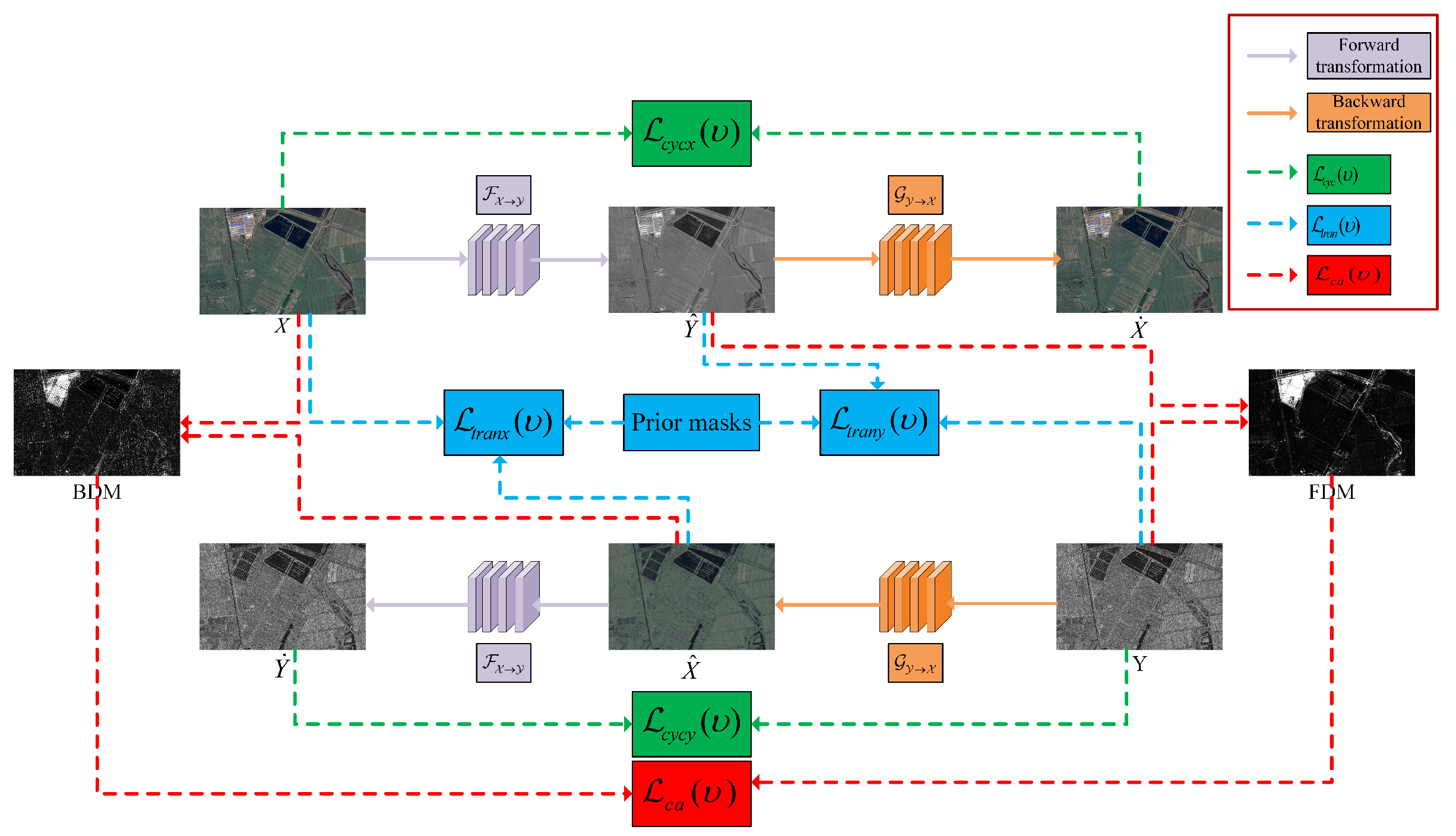
The specific transformation process of this network is illustrated in Figure 1, where the solid lines represent the process of image transformation, and the dashed lines in various colors represent the calculation of different objective functions. X is transformed into the domain by the forward transformation function to obtain the transformed image . The transformed image is subsequently transformed back to the domain by the backward transformation function and then the cyclic image is obtained. Similarly, Y can be transformed to domain by to obtain the transformed image , and then the transformed image can be transformed back to domain by to obtain the cyclic image . The training optimization of the networks and are optimized by backpropagation minimizing the weighted transformation objective function , cyclic consistency objective function , and change alignment objective function . By constraining the network transformation process through these objective functions, the image can be well transformed to the target domain. Meanwhile, it can maintain the information of the source domain image, as well as reduce the complementary information of the FDM and BDM, thus improving the final CD effect.
The following is a detailed description of each part of the network, respectively.
2.1.1. Prior Mask Generation
In order to reduce the impact of changing regions on the training of and , we design a strategy to generate the forward and backward prior masks based on the IRG-McS [26].
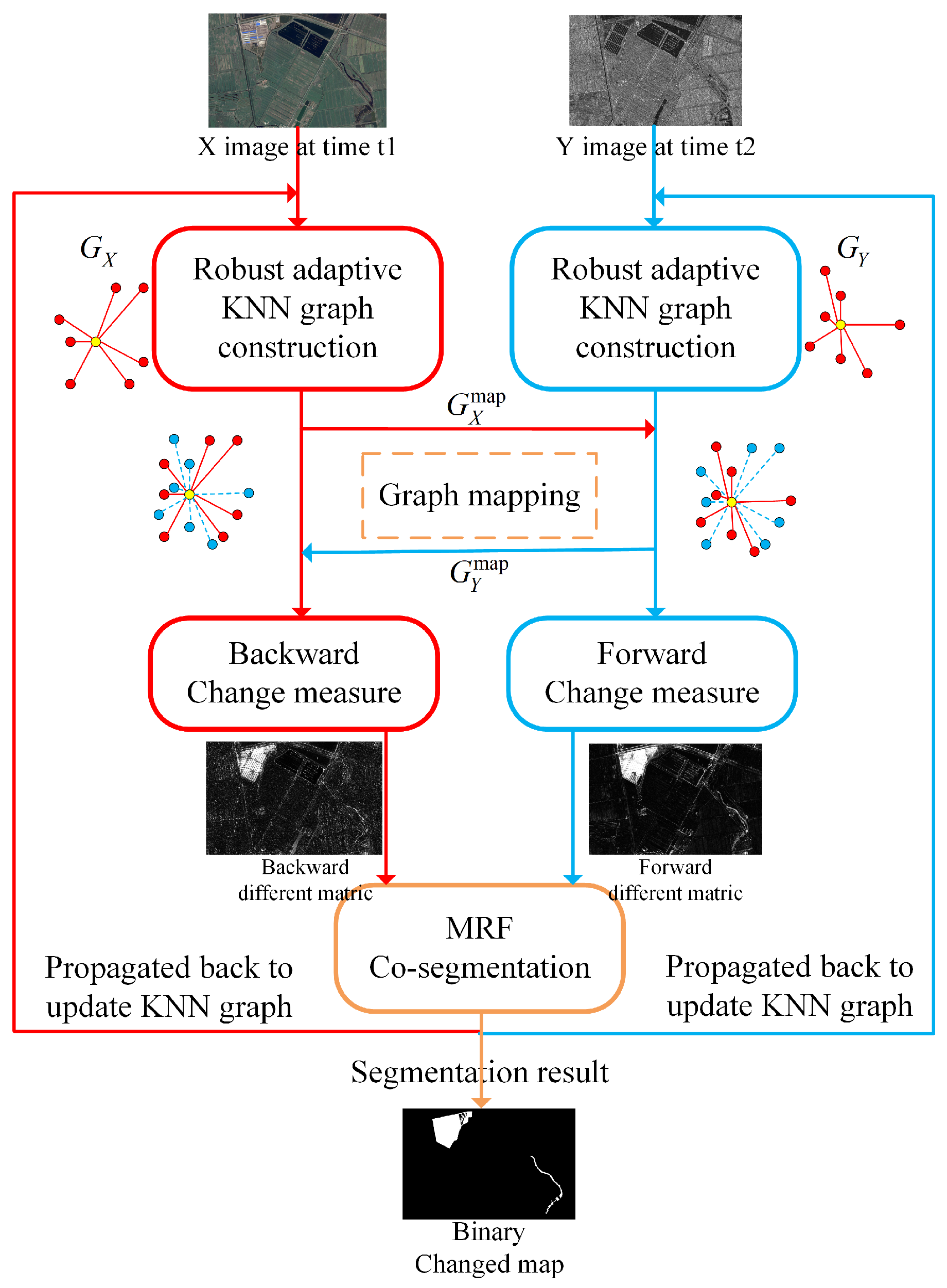
IRG-McS utilizes the characteristic that heterogeneous images share the same structural information of the same geographical object. Firstly, robust K-nearest neighbors graphs are constructed to represent the structure of each image. Then the graph structures of different domains are mapped to the same graph structure space using graph mapping. The graph structures in the same space are compared to calculate the forward and backward difference matrices. In this way, it avoids the confusion of heterogeneous data as in the similar affinity matrix, and thus improves the quality of the difference matrices. The Markov co-segmentation model has then been used to segment the forward and backward difference matrices, which initially detect the changed regions. Once Markov co-segmentation detects the changed regions, they are propagated back to the graph construction process to reduce the effect of neighborhood point changes. This iterative framework generates more robust prior forward and backward difference matrices by providing more robust graph structures. The schematic diagram of IRG-McS is shown in Figure 2.
IRG-McS generates simple and efficient prior difference matrices, which are better than the prior difference matrices in X-Net, ACE-Net, CAA, and other methods. We generate the prior masks by hard segmentation of the different matrices, which can better reduce the impact of the change regions on the transformation network. The details are as follows. The corresponding backward thresholds and forward thresholds are obtained by Otsu [40] segmentation for the prior backward difference matrix and forward difference matrix. When the value of the corresponding pixel in the prior backward difference matrix is larger than , assign the pixel the value 0. In contrast, when the value of the corresponding pixel in the prior backward difference matrix is less than the pixel will be assigned the value of 1. The backward mask is obtained from the prior backward difference matrix by hard segmentation. The same operation is done for the prior forward difference matrix to obtain the forward mask . The and guide the image transformation to minimize the negative impact of change regions which can improve CD performance.
However, IRG-McS still has the following three problems. First, the graph structure constructed by IRG-MCS is not robust enough when the input of IRG-McS is a heterogenous image of a complex scene. This will result in generated difference matrices that are not robust enough. Meanwhile, the limitation of the segmentation algorithm will lead to false positives (FP) and false negatives (FN) in the binary change map. Second, the process of obtaining the difference matrices by IRG-McS is all linear operations, resulting in the poor learning ability of IRG-McS. Therefore, IRG-McS is combined with the nonlinear transformation functions and to improve the CD performance of IRG-McS. Third, it is only able to obtain the final difference and binary change maps in IRG-McS, which is sufficiently useful for the simple detection of changes. Nevertheless, it is not possible to visually represent the changes between before and after moments of heterogeneous images. With IRG-McS, it can only be known that changes have occurred, without being able to visually see what type of change has occurred. The method based on deep transformation networks is able to obtain before-and-after moment images of the same domain, which allows us to visually indicate the type of change.
In conclusion, combining IRG-McS with the deep transformation network can improve both the network transformation and the quality of the difference matrices. On the one hand, it can well-reduce the negative effect of the change regions on the network training to improve the quality of the final binary change map. On the other hand, the transformation network enables us to visualize the changes in the same domain.
2.1.2. Forward and Backward Transformation
In order to make heterogeneous images comparable, we transform heterogeneous images into homogeneous images through forward and backward transformation processes. To ensure that and can efficiently transform the heterogeneous images from the source domain to the target domain, the forward and backward transformation processes need to satisfy the following constraints.
However, for the CD task, there are change regions in the before- and after-moment images. If the change regions are involved in the forward and backward transformation process of the network, and will learn a trivial solution that maps the changed regions to unchanged regions at the same location in another domain. Therefore, we combine the and generated by IRG-McS with the constraints of (2) to produce a weighted transformation objective function, which can reduce the negative impact of the change regions by constraining and . In particular, and , respectively, transform the image to the and domains. The and are constructed in and domains, respectively, which naturally differ and have the information of corresponding domains. Through an opposite guidance process of to guide and to guide , which enables the network to learn more information about the changes.
When the heterogeneous image pairs X and Y are from different optical sensors (such as X from Worldview2, Y from Pleiades), the distributions of X and Y are approximately Gaussian [41], so the mean square error (MSE) formula is utilized to constrain the forward and backward transformations as shown in (3). X, , Y, , and are expanded into one-dimensional vectors for the calculation.
where are the i-th pixels in X and , respectively, are the i-th pixels in Y and , respectively, are the i-th pixels in and , respectively, , and represents the -norm.
However, when the heterogeneous image pairs X and Y are from optical and SAR sensors, respectively (such as X from Landsat-8, and Y from Sentinel-1A), the effect of multiplicative coherent speckle noise exists in Y. Therefore, the log-ratio operator [15] is introduced in the domain to constrain the backward transformation as shown in (4).
Equations (3) and (4) enable the image transformed from the source domain through the target domain to maintain the same pixel values in the unchanged regions as the pixel values of the image in the target domain at another moment. Meanwhile, MSE is weighted by the and , thus avoiding the effect of changing pixels on network training. However, there may be false checks and missed checks in and , so and are updated when the transformation network is trained to a certain number of epochs. This iterative update process can avoid the transformation network to be completely dependent on and , thus improving the stability of the transformation network. Overall, the weighted transformation objective function enables the transformed image to approximate the image of the real target domain, which improves the quality of the final binary change map.
2.1.3. Cyclic Consistency Transformation
The purpose of the forward and backward transformations is to constrain the distribution of the transformed image () to be identical to the target domain image X (Y) in the unchanged region. However, it does not consider that the transformed image () has to keep the same information as the source domain image Y (X). Therefore, we consider introducing the cyclic consistency transformation process in CycleGAN [42]. Both forward and backward cyclic transformations are performed to ensure that the transformed images and maintain the information of their respective source domain, as shown in (5).
Similar to the analysis of the specific formula for the weighted transformation objective function, the cyclic consistency the objective function is also divided into two cases. When X and Y are from different optical sensors, the specific calculation is shown in (6). X, , Y, and are also expanded into one-dimensional vectors for the calculation.
where and are the i-th pixels in and , respectively, .
However, when X and Y are from optical and SAR sensors, respectively, the cyclic consistency objective function is calculated as shown in (7).
The cyclic transformation objective function can constrain and to transform back to the source domain after transforming to the target domain. It ensures that and have the identical distribution of the target domain and the identical information of the source domain image.
2.1.4. Change Alignment Process
and can ensure to some extent that the network transformation obtains the accurate transformed images and . Then, we can obtain the BDM () and FDM () as follows.
where are the i-th elements in the and , respectively, .
However, there are two factors that limit the ability to indicate the area of change simply on the basis of and . First, the network is limited by the quality of the prior masks as well as the learning ability, which leads to the difference between () and the true representation of X in the domain (the true representation of Y in the domain), thus and are not the same as the true change. Second, and are, respectively, calculated in the domain and domain, which both carry domain-specific information. According to the above two factors, the previous methods fuse the and with complementary information to obtain the fused difference map after the network training is completed. This fusion strategy only improves the quality of the final change map to some degree, but it cannot fundamentally affect the image transformation effect to improve the CD performance. Therefore, we design a change alignment process in the network transformation to fuse and . It enhances the effect of image transformation and thus fundamentally improves the quality of the final binary change map.
The change alignment process is achieved by optimizing the change alignment objective function, which is implemented as follows. and are multiplied pixel by pixel, and then averaged and inverted to obtain the final change alignment objective function value, as shown in (9). and are also expanded into one-dimensional vectors for the calculation.
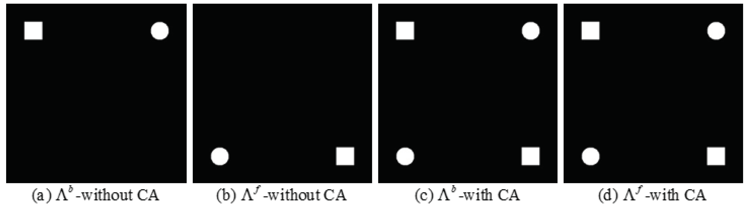
will enable the and to indicate the same region of change, as shown in Figure 3.
Figure 3 illustrates the hypothetical case with and without the change alignment process. There are differences between and when the transformation network has no change alignment process. After the change alignment process is introduced in the transformation network, and trend towards the same. However, if there are false positive regions in the change map obtained by and , the network simply by the constraint will make the false positive regions more certain to be detected as change regions, which results in degraded CD performance. Therefore, we constrain the transformation network jointly by , and , as shown in (10).
where and are the weights of each objective function, which are used to balance the influence of each objective function on the network training.
The training process optimizes the network by minimizing the full objective function with the network parameters as independent variables. Two reasons why the joint constraint network can facilitate the positive impact of on transformation are explained as follows. On the one hand, and have an adversarial process in the unchanged region in and . reduces the value of the elements in and to limit the effect of on unchanged regions, while enables the network to detect missed changes in and by increasing both the value of the elements in and . On the other hand, constrains the network forward and backward transformation effects by the cyclic transformation process on all regions, which makes the does not affect the transformation effect unrestrictedly. The constraints on by and enable to utilize the information of and to positively improve the network transformation effect.
2.2. Obtain the Final Difference Map and Binary Change Map
After the training of the network is completed, X and Y are input into the network to obtain the desired and . Then the final and can be obtained in the and domains, respectively. Although the change alignment can utilize the complementary information of and in the network transformation process, there is still domain-specific information in the final and . Therefore, we simply fuse the and after the network training to obtain the fused difference map (), which can improve the CD performance.
where stands for taking the maximum value in the difference map. The quality of will be reduced because of the outliers in and , which affect their normalization. For this reason, it is generally important to crop the pixels whose pixel values exceed three standard deviations from the mean in and , respectively.
Once the is obtained, the CD task can be modeled as a binary classification problem. It aims to obtain the changed and unchanged pixels from the final difference map, which is indicated by 1 for changed pixels and 0 for unchanged pixels. In this paper, the PCA-Kmeans [39] method is chosen to obtain the final binary change map. Firstly, we construct the feature vector space of by PCA. The Kmeans algorithm with is then used to cluster the feature vector space into two clusters that correspond to changed and unchanged. Finally, the binary change map is generated by assigning each pixel of to one of the two clusters.
3. Experimental Results
This section initially introduces five real datasets commonly used in heterogeneous CD task. Then the experiment setup is specified. It is followed by showing the experimental results of CACD and state-of-the-art comparison methods on these datasets to illustrate the effectiveness and superiority of CACD. Finally, an ablation study on different datasets is conducted to evaluate the effectiveness of the different modules of CACD.
3.1. Datasets
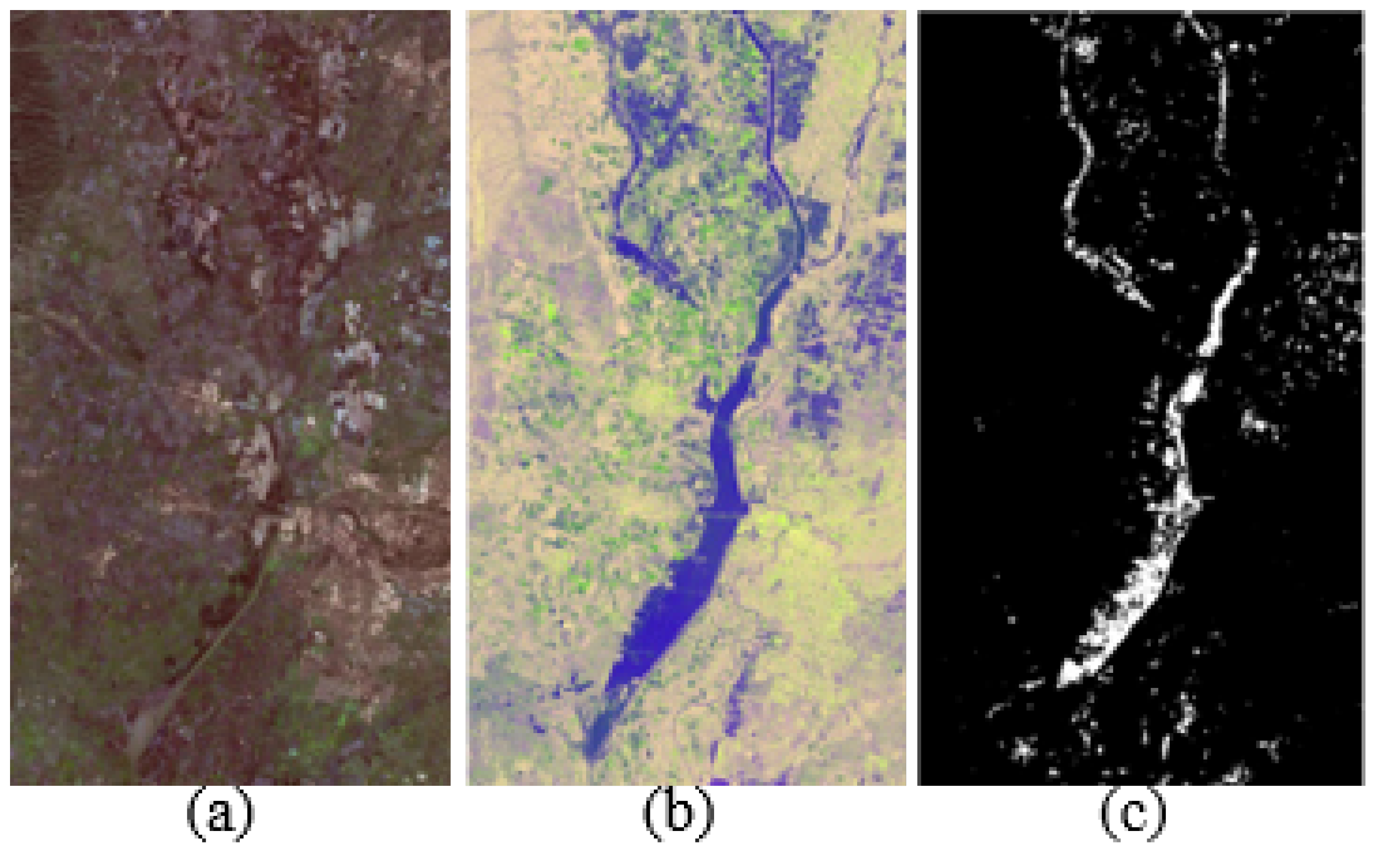
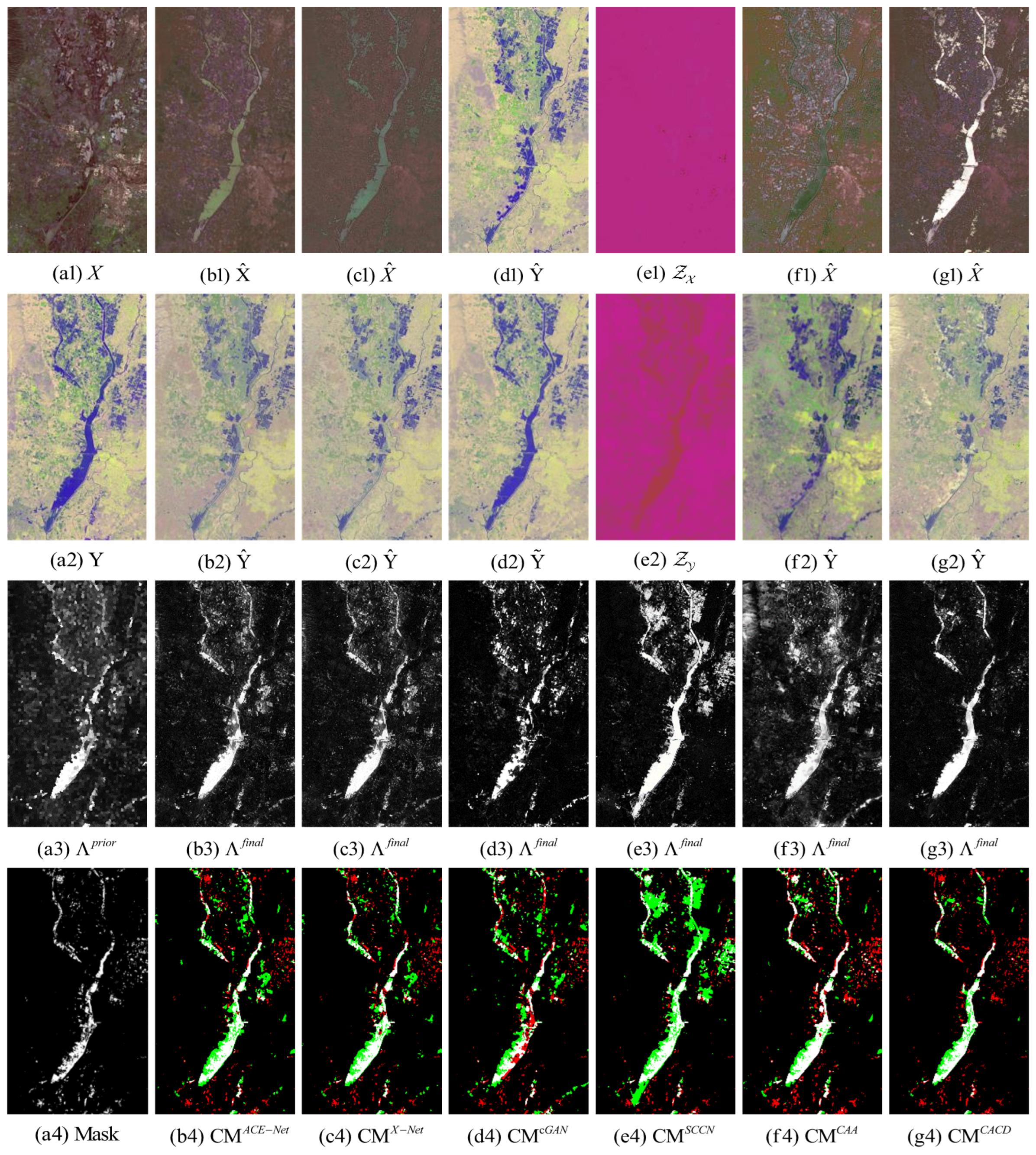
1. California dataset: This dataset shows the disaster in Sacramento, Yuba, and Sutter counties in California before and after the flooding. The image before the disaster is shown in Figure 4a, which is an optical image obtained by Landsat-8 in January 2017. The image after the disaster is shown in Figure 4b, which is a polarized SAR image obtained by Sentinel-1A in February 2017. The image size and spatial resolution are and 15 m, respectively. Figure 4c indicates the ground truth change of these two images [31].
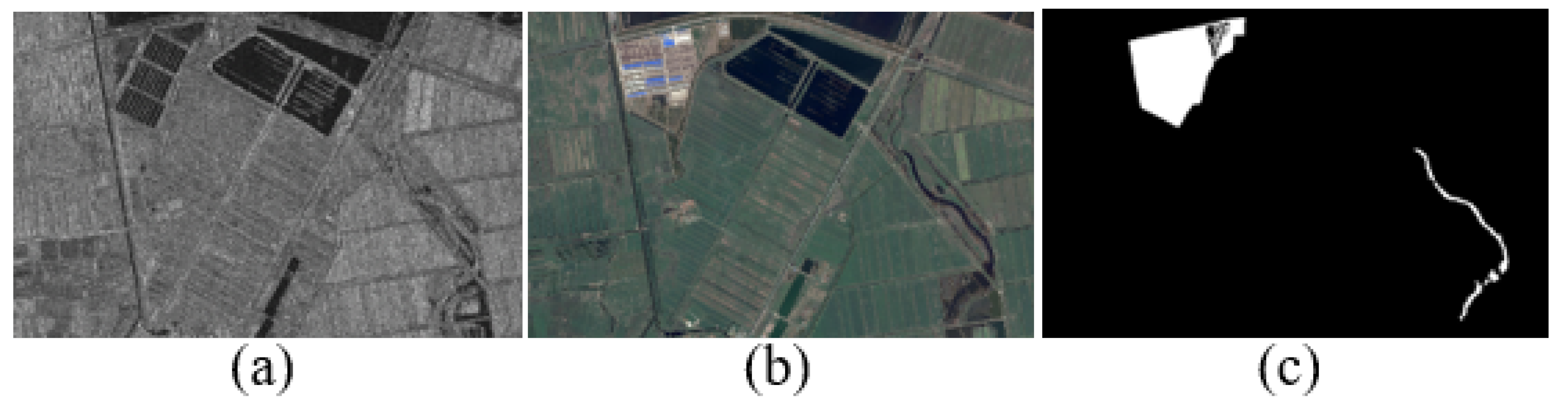
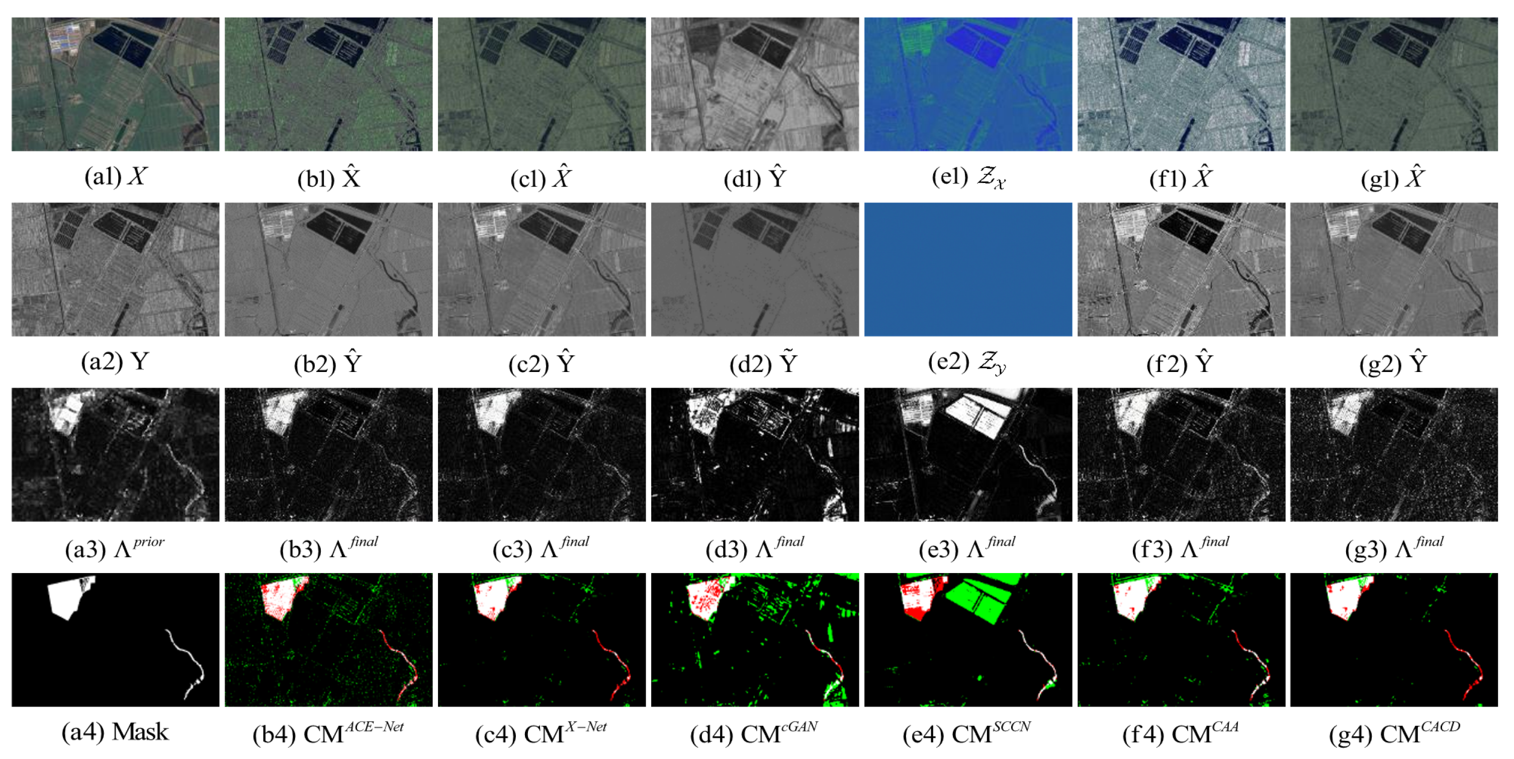
2. Shuguang dataset: It consists of SAR image and optical image, as shown in Figure 5a,b, respectively. The two images were acquired in Shuguang village, Dongying, China, with a spatial resolution of 8 meters and a dimensional size of . The SAR image was taken in June 2008 by Radarsat-2, while the optical image was taken in September 2012 by Google Earth. Figure 5c represents the ground truth change of these two images.
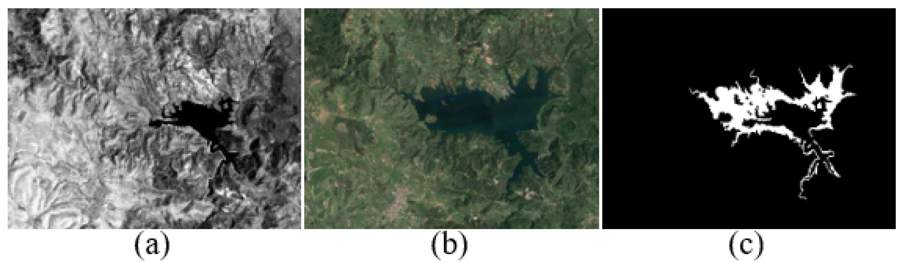
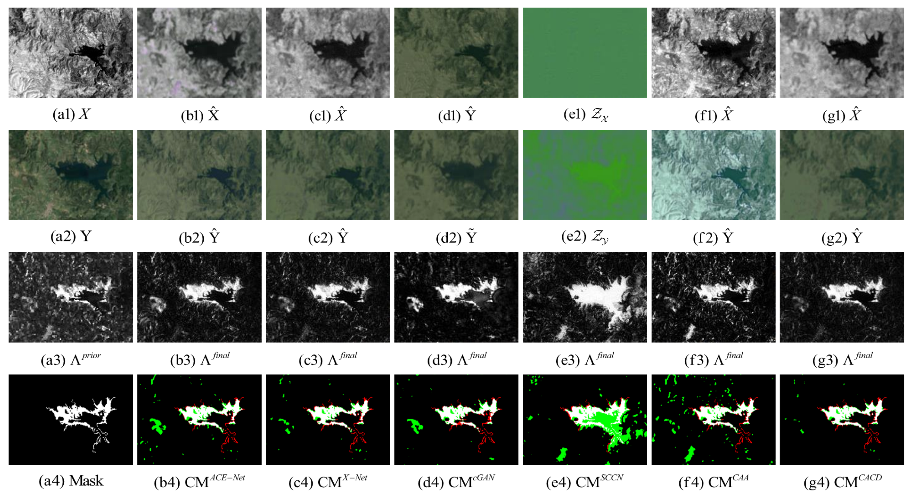
3. Sardinia dataset: This dataset shows the changes before and after the lake flooding in Sardinia, Italy. Figure 6a shows an image in the near-infrared band acquired by the Landsat-5 satellite in September 1995. The optical image of Figure 6b was acquired by Google Earth at the same location in July 1996. They both have the same 30 m spatial resolution and size. The real change situation on the ground is shown in Figure 6c.
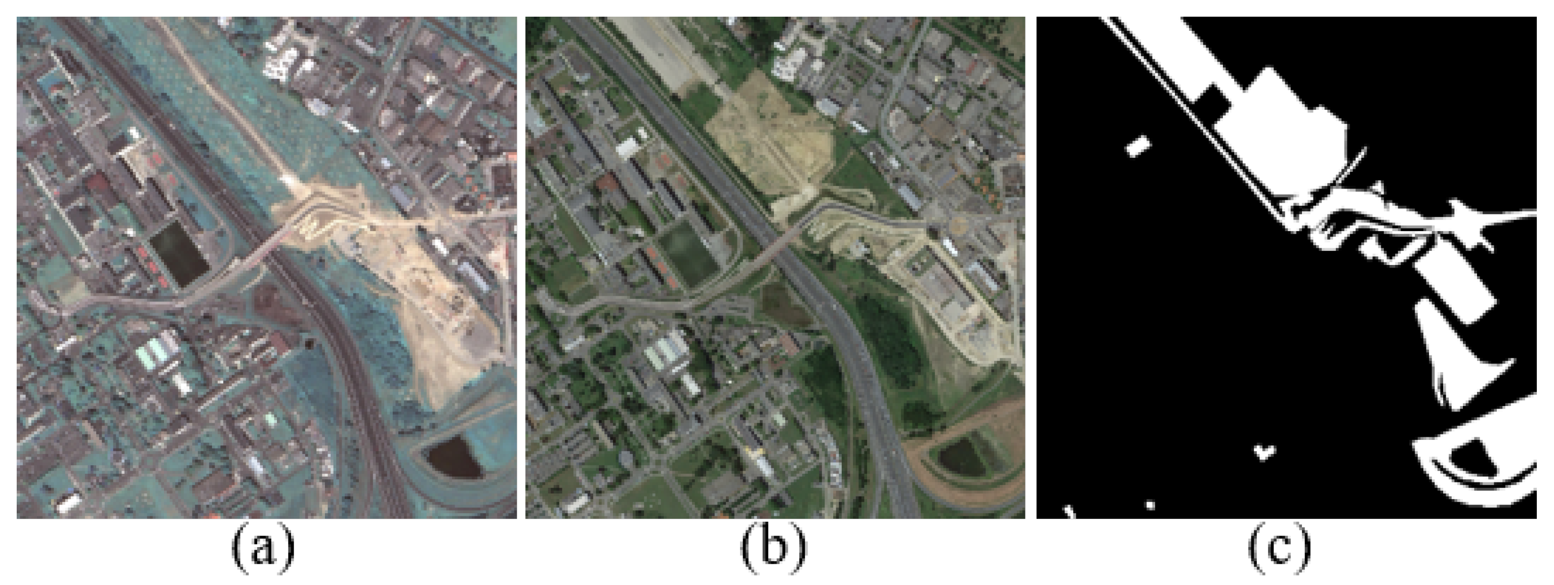
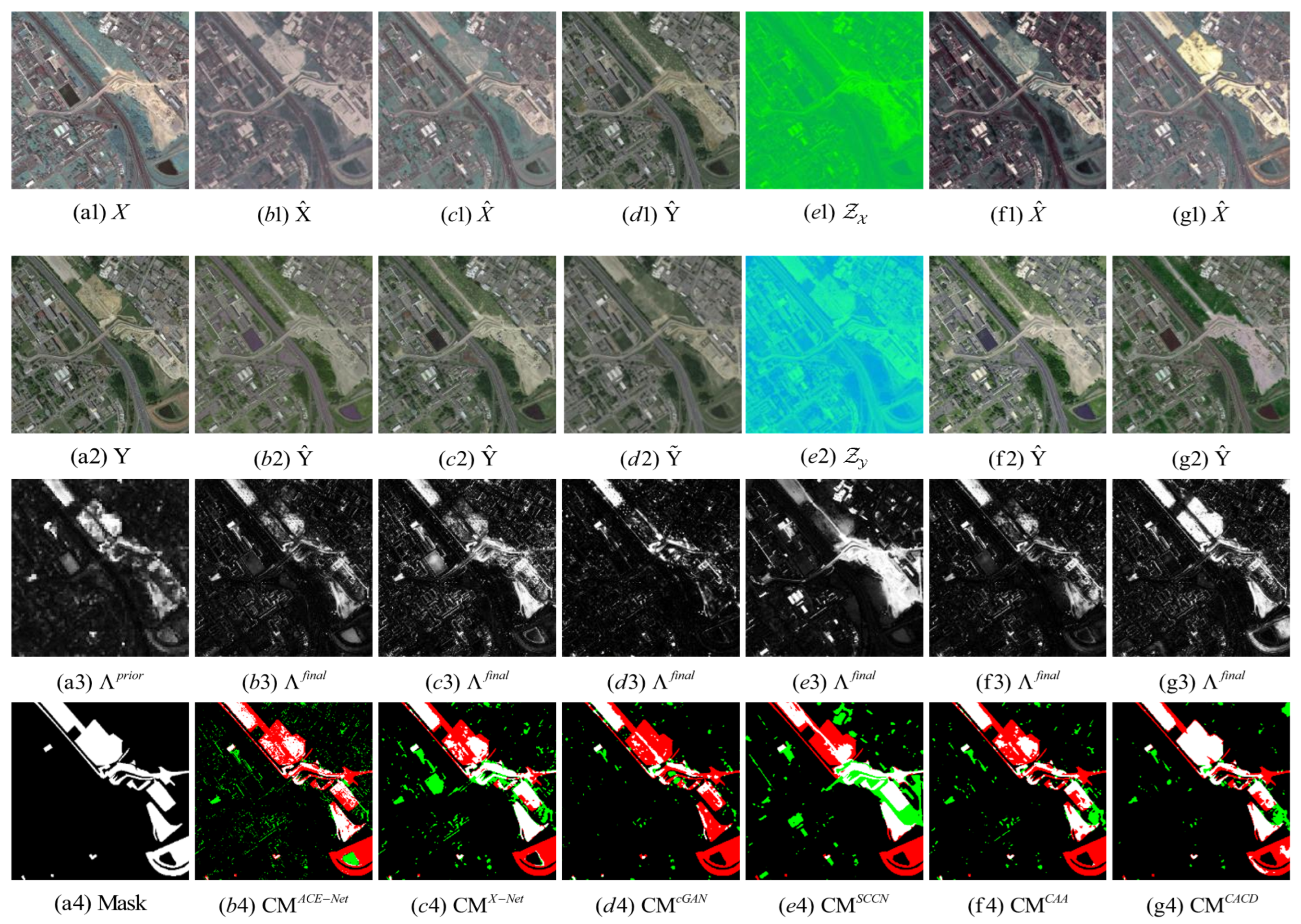
4. Toulouse dataset: This dataset shows the progress of road construction work in Toulouse, France, between May 2012 and July 2013. It consists of two optical images acquired by Pleiades (Figure 7a) and WorldView2 (Figure 7b). The basic truth in Figure 7c describes this change. The image size and spatial resolution are and 0.5 m, respectively.
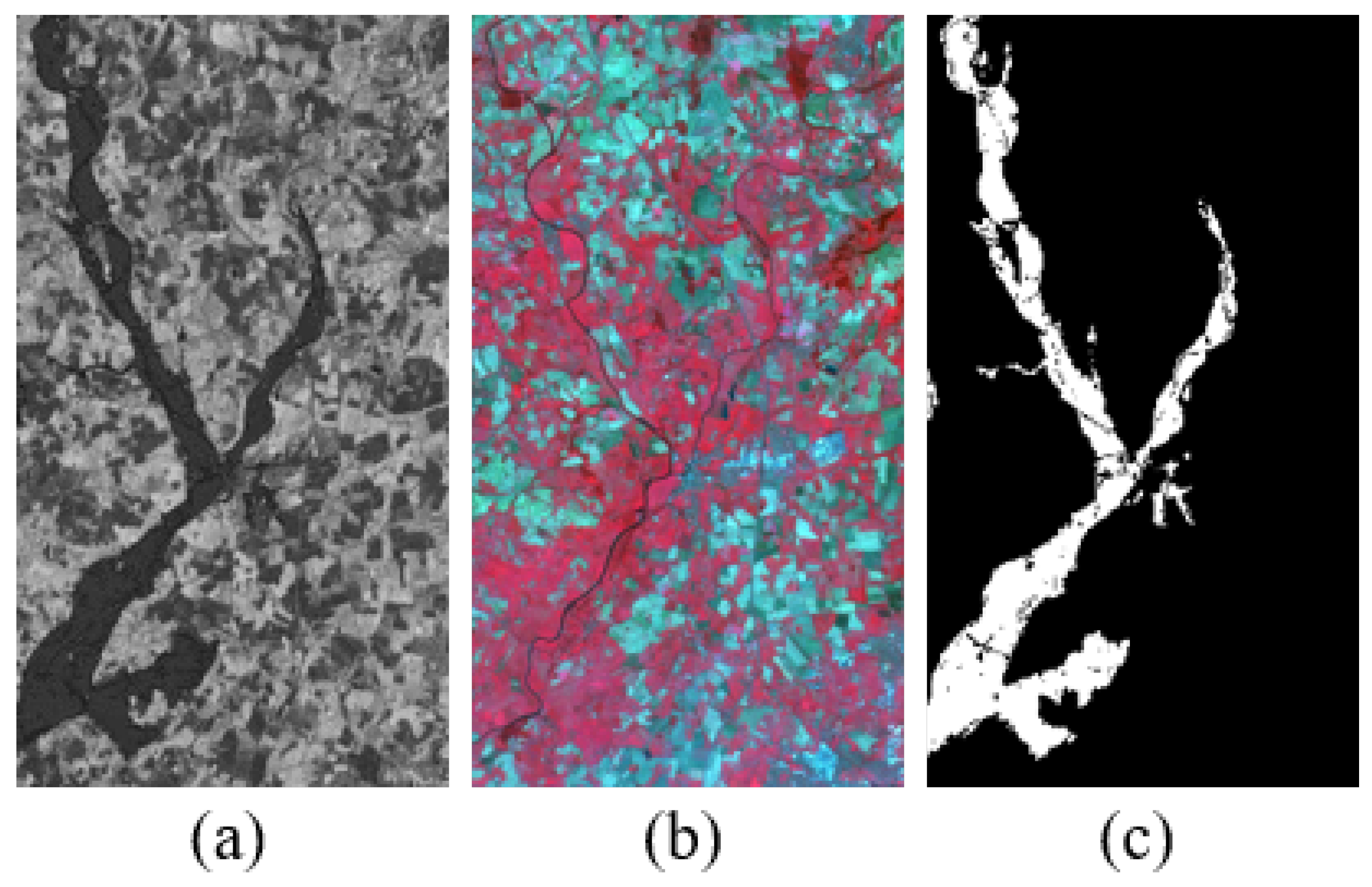
5. Gloucester dataset: This dataset shows the changes before and after the lake flooding in Gloucester, England. The ERS image was captured in October 1999 as shown in Figure 8a. The SPOT image composed of three spectral bands, as shown in Figure 8b, was obtained at the same location in 2000. They both have the same 25 m spatial resolution and size. The real change situation on the ground is shown in Figure 8c.
3.2. Experimental Setup
The experimental configuration is based on NVIDIA 1050Ti GPU, which is used on windows system, and the experiments are implemented by Tensorflow 1.8.0 framework under python language.
In this paper, the network framework is based on X-Net [36], which consists of two CNNs and composed of four fully convolutional layers. The two CNNs and have the same structure, but do not share parameters. The number of convolution kernels from the first to the last layer is 100, 50, and 20, and the channel number of the target domain image, where the convolution kernel size is . The LeakyRelu function [43] is chosen for the activation function of the initial three layers, while the slope of the negative independent variable is set to . The activation function of the last layer is chosen as hyperbolic tangent function because the input images are normalized to . The dropout layer is inserted after each convolutional layer, and the dropout rate is set in the training phase to drop the neurons to prevent over-fitting [44].
The backward propagation process chooses the Adam optimizer [45] to optimize the network by minimizing the objective function at a learning rate of . The weights of the three objective functions are set to , and is determined based on different datasets. The number of training epochs of the network is set to 160, and each epoch contains 10 batches, which are composed of 10 patches of size . When the network iterates to 60 and 120 epochs, X and Y are input to the network to obtain the transformed and . Then and are calculated and and are obtained by hard segmentation of the Otsu threshold. It updates prior and obtained by IRG-McS in order to reduce the effect of changing regions on network training more effectively.
In this paper, state-of-the-art unsupervised CD methods are chosen as the comparison experiment. That is, ACE-Net [36], X-Net [36], cGAN [35], SCCN [27], CAA [37] and IRG-McS [26] comparison methods, which are detailed in the introduction section. In order to effectively evaluate the superiority of the proposed method CACD, overall accuracy (OA), score, Kappa coefficient (Kc) [46], and the area under the curve (AUC) are selected for the comprehensive evaluation in this paper.
3.3. Results
In this section, the proposed CACD and the comparison methods ACE-Net, X-Net, cGAN, SCCN, CAA and IRG-McS are illustrated for image transformation results on different datasets and their evaluation criteria results. In order to reveal the comparability of the results, the binary change maps of the above methods are obtained by PCA-Kmeans method. IRG-McS is not based on image transformation, thus making the comparison of its evaluation criteria merely to evaluate the effectiveness of the network in enhancing the prior and .
3.3.1. Quantitative Evaluation
Table 1, Table 2, Table 3, Table 4 and Table 5 show the evaluation criteria, AUC, OA, Kc, and , for the proposed and compared methods on the California, Shuguang, Sardinia, Toulouse and Gloucester datasets, respectively. From Table 1, Table 2, Table 3, Table 4 and Table 5, it can be seen that the proposed CACD achieves the best results for different datasets, and the average of the evaluation criteria obtained for different datasets obtains AUC, OA, Kc, and of 96.2%, 95.9%, 77.0%, and 79.2%, respectively. It improves the average evaluation criteria AUC, OA, Kc, and by 2.0%, 1.25%, 6.8%, and 6.2%, respectively, over the second-best method (X-Net) on different datasets. This demonstrates the superiority of the proposed CACD with great improvement over the method with the same network framework. It benefits from the robust prior and generated by using IRG-McS to guide the network for training, avoiding the influence of changing regions on the deep transformation network. Moreover, it benefits from the change alignment process in the image transformation, which reduces the difference between the and by constraining them during the network training. Thus, the quality of the is improved and ultimately the performance of CD is improved. The proposed CACD improves the average evaluation criteria AUC, OA, Kc, and on different datasets by 2.95%, 1.1%, 12.7%, and 11.4%, respectively, over the IRG-McS method that generates the forward and backward difference matrices. It can be seen that combining the prior difference matrices with the transformation network can improve the quality of the prior difference matrices, which improves the performance of CD.
3.3.2. Qualitative Evaluation
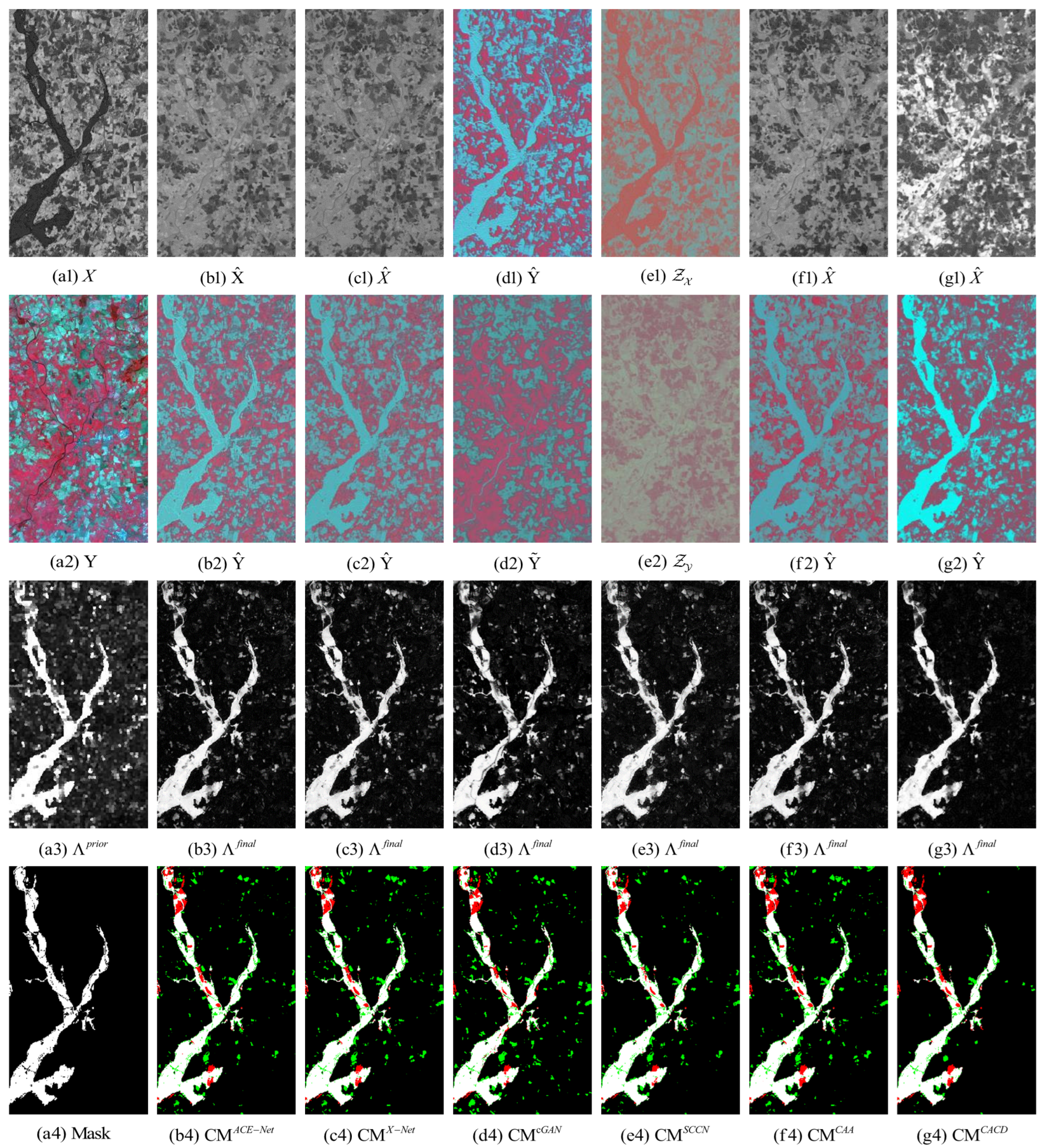
The following illustrates the visualization of the image transformation effect and the difference map and binary change map of the proposed method and the five methods of ACE-Net, X-Net, cGAN, SCCN, and CAA on five heterogeneous CD datasets. The results of image transformation on the California, Shuguang, Italy, Toulouse and Gloucester datasets are illustrated in Figure 9, Figure 10, Figure 11, Figure 12 and Figure 13. IRG-McS is not shown here because the method is not performed based on image transformation.
The superior performance of the proposed method in this paper on all five datasets can be seen from the result. Firstly, it can be observed from the image transformation results that the transformed image obtained by the proposed CACD is closer to the real image in the target domain. It maintains both the texture as well as the information of the source domain and has similar statistical properties as the target domain. Thus, the transformed image can be compared directly with the image of the target domain. Then, from the difference map and binary change map results, it can be seen that the results obtained from the proposed CACD are more closely matched to the real change region. The regions of FN and FP are relatively small compared to other methods. The affinity matrices in X-Net, ACE-Net, and CAA do not provide a good indication of the changed and unchanged regions. It causes the change regions to negatively affect the training of the deep transformation network, which can damage the effectiveness of the network transformation and the quality of the final change map. There are two reasons for the superior performance of the proposed CACD. (1) A more robust IRG-McS method for generating a difference matrix is chosen to replace the affinity matrix, which generates prior masks that are better for reducing the influence of the change region on the deep transformation network. (2) By introducing the change alignment process in the network training process, the and are constrained in a way that the two-way difference map approximates the real change condition, which is used to improve the quality of the final change map.
3.4. Discussion
3.4.1. Ablation Study
To verify the validity of the change alignment process and the robust prior masks, an ablation study is performed on four datasets correspondingly to evaluate the contribution of each component to the performance. The following experiments are conducted under different network configurations.
- (1).
- Proposed: CACD.
- (2).
- No change alignment process.
- (3).
- No prior masks: by randomly initializing a difference map.
- (4).
- Neither change alignment process nor the prior masks.
It can be seen from Table 6 that for the Toulouse dataset, the change alignment process is very effective. By comparing configuration (1) and configuration (2), we find that configuration (1) improved 4.2%, 2.5%, 8%, and 6.6% in the evaluation criteria AUC, OA, Kc, and , respectively, which is a great improvement.
However, when comparing configuration (1) and configuration (3), it is found that the improvement of configuration (1) over configuration (3) for the evaluation criteria is only 0.7%, 1.4%, 2.6%, and 2%, respectively, which is not a very obvious improvement. Because during the network iteration, the prior masks are iteratively updated at a specific number of epochs to improve the quality of the prior masks, the prior masks generated by randomization are not very good at the beginning of network training to mitigate the effect of changing regions on network training. Nevertheless, after the network has been iterated for a certain number of epochs, it is able to give a good indication of the change regions. Thus, the performance of CD can be improved by updating the prior masks. When the quality of the prior masks obtained from the iterative update of the network and the quality of the prior masks obtained from IRG-McS are similar, and the quality of the final change map obtained is not far from each other.
The next comparison is between configuration (2) and configuration (4), with neither change alignment process. Generating the prior masks by IRG-McS to guide the network training improved 2.5%, 1.8%, 6.8%, and 5.5% over the randomly generated difference matrix to guide the network training on the evaluation criteria, respectively. It illustrates that guiding network training by a randomly generated difference matrix without the change alignment process cannot overcome the limits of the transformation network. It can be seen that the more robust prior masks are effective for the training of the network.
Comparing configurations (3) and (4), both are trained by the randomly generated prior difference matrix guiding the network. The improvement in the change map obtained for the configuration with change alignment process constrained network training over the configuration without change alignment process is 6%, 3.2%, 12.2%, and 12.1% on the evaluation criteria, respectively. The superiority of the change alignment process can be seen from the fact that it is equally effective in obtaining good change maps even when the prior masks are randomly generated.
The results in Table 7, Table 8 and Table 9 for the California, Shuguang, and Sardinia datasets, respectively, also reflect the results obtained from the above analysis. In summary, the results of the ablation study on four different datasets show the effectiveness of the robust prior masks and change alignment process in the CACD method, especially the superiority of the change-alignment process. Without the robust prior masks, the same good performance can be obtained by introducing the change alignment process and updating the prior masks by network iteration.
3.4.2. Parameter Analysis
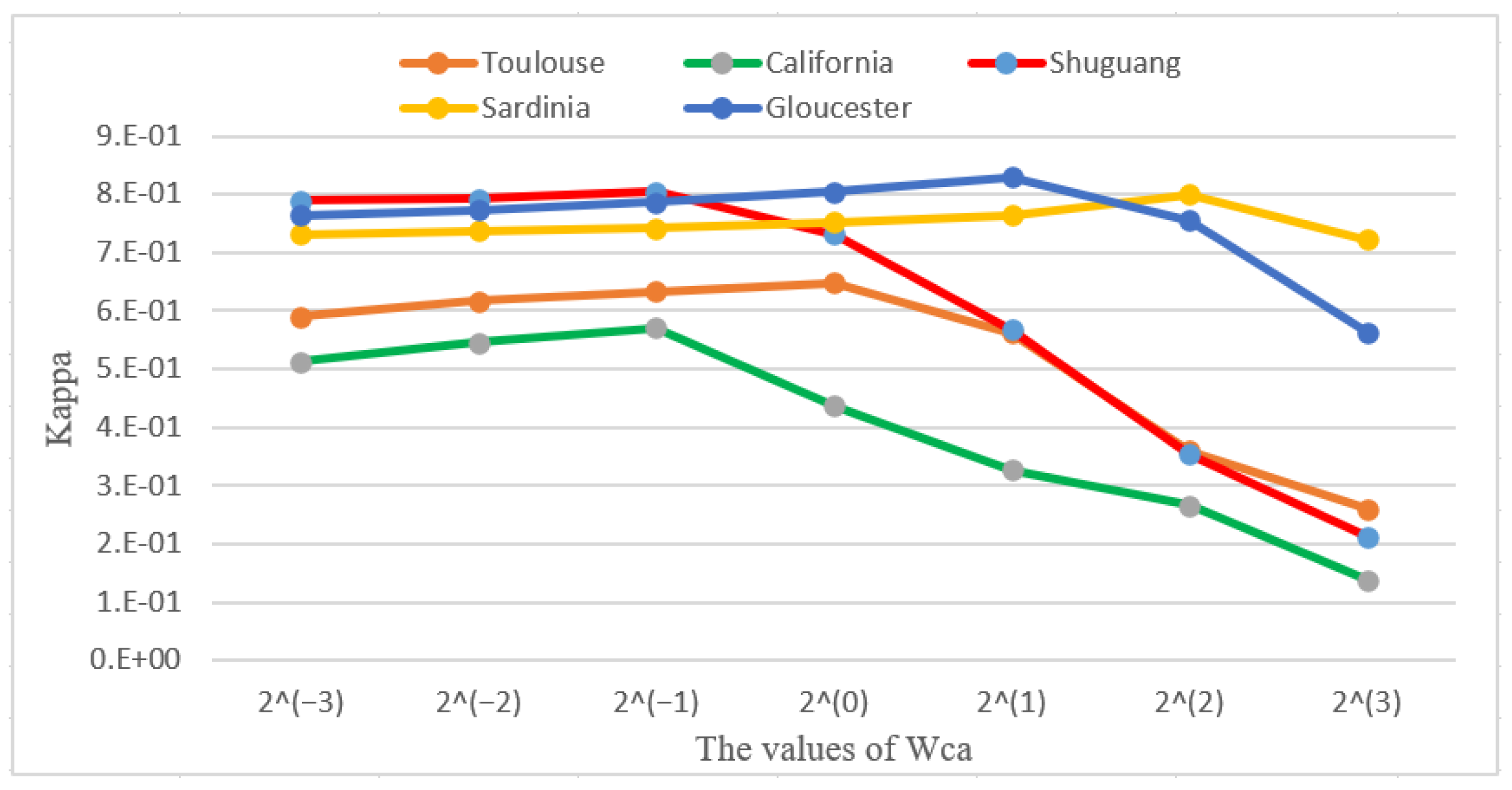
The effectiveness of the change alignment process can be seen from the results of the ablation experiments. The change alignment process is carried out by the joint constraint of , and on the network. The joint constraint then has a problem of balancing the effect of different objective functions on the network, so we assign different weight values to different objective functions to balance their effect on the network. To better understand the role of the change alignment process, we adjust the weight parameter of on different datasets to observe the experimental results. The experimental results are shown in Figure 14.
Figure 14 shows the influence of from to on Kappa coefficient, and the lines in different colors correspond to the five used datasets, respectively. It can be seen from the Figure 13 that, when different weights are set for , there is a large difference in the change detection performance for different weights. When the value of increases gradually from small to large, the performance of change detection becomes gradually better. This is because at this stage plays an active role in network transformation, and thus enables fewer false negatives in the final change map. After the Kappa coefficient reaches its peak, the performance of change detection decreases sharply as the value of increases. This is because the constraints of and in the network are not enough to balance the effect of in the network at this time, which can lead to an increase in the number of false positives detected and thus reduce the change detection performance.
3.4.3. Time Efficiency Analysis
Time efficiency is also an important aspect of the algorithm. For unsupervised change detection methods, they require a separate processing time for different data. Therefore, we calculate the running time on different data sets for CACD and some other comparison methods. The experimental results are shown in Table 10.
It can be seen from Table 10 that the traditional IRG-McS algorithm has the shortest running time. This is because IRG-McS is based on linear operations with lower time complexity compared to the deep learning methods. Our proposed CACD method is based on the X-Net framework, but the running time of CACD is substantially reduced compared to X-Net. This is because we choose a more efficient strategy than the affinity matrix in X-Net to reduce the influence of the change regions.
4. Conclusions
In this paper, we propose a CD framework for heterogeneous images based on change alignment. Firstly, the proposed CACD method generates the prior masks based on the graph structure to unsupervised guide the transformation network training, which reduces the negative impact of changing regions. Then, the change alignment process is introduced during the network training. It is the first time that the transformation network exploits the complementary information of FDM and BDM, which can influence the transformation effect and thus radically improve the quality of the final difference map. Finally, the change map is obtained by the PCA-Kmeans clustering method for the images transformed into homogeneous sources. The experimental results show that the proposed CACD outperforms other state-of-the-art methods in terms of performance. In future work, we will consider domain alignment to fuse FDM and BDM and thus make better use of the complementary information between them to improve the CD performance.
Author Contributions
Methodology, K.X.; software, K.X. and Y.S.; validation, K.X., L.L. and Y.S.; original draft preparation, K.X.; writing—review and editing, Y.S.; supervision, L.L. and Y.S. All authors have read and agreed to the published version of the manuscript.
Funding
This research was funded by Natural Science Foundation of Hunan Province, China of grant number 2021JJ30780.
Institutional Review Board Statement
Not applicable.
Informed Consent Statement
Not applicable.
Data Availability Statement
Not applicable.
Conflicts of Interest
The authors declare no conflict of interest.
References
- Singh, A. Review Article Digital change detection techniques using remotely-sensed data. Int. J. Remote Sens. 1989, 10, 989–1003. [Google Scholar] [CrossRef] [Green Version]
- Wen, D.; Huang, X.; Bovolo, F.; Li, J.; Ke, X.; Zhang, A.; Benediktsson, J.A. Change Detection From Very-High-Spatial-Resolution Optical Remote Sensing Images: Methods, applications, and future directions. IEEE Geosci. Remote Sens. Mag. 2021, 9, 68–101. [Google Scholar] [CrossRef]
- Lv, Z.; Liu, T.; Benediktsson, J.A.; Falco, N. Land Cover Change Detection Techniques: Very-high-resolution optical images: A review. IEEE Geosci. Remote Sens. Mag. 2022, 10, 44–63. [Google Scholar] [CrossRef]
- Bai, B.; Fu, W.; Lu, T.; Li, S. Edge-Guided Recurrent Convolutional Neural Network for Multitemporal Remote Sensing Image Building Change Detection. IEEE Trans. Geosci. Remote Sens. 2022, 60, 1–13. [Google Scholar] [CrossRef]
- Kennedy, R.E.; Townsend, P.A.; Gross, J.E.; Cohen, W.B.; Bolstad, P.; Wang, Y.; Adams, P. Remote sensing change detection tools for natural resource managers: Understanding concepts and tradeoffs in the design of landscape monitoring projects. Remote Sens. Environ. 2009, 113, 1382–1396, Monitoring Protected Areas. [Google Scholar] [CrossRef]
- Brunner, D.; Lemoine, G.; Bruzzone, L. Earthquake Damage Assessment of Buildings Using VHR Optical and SAR Imagery. IEEE Trans. Geosci. Remote Sens. 2010, 48, 2403–2420. [Google Scholar] [CrossRef] [Green Version]
- Lv, Z.; Wang, F.; Cui, G.; Benediktsson, J.A.; Lei, T.; Sun, W. Spatial-Spectral Attention Network Guided with Change Magnitude Image for Land Cover Change Detection Using Remote Sensing Images. IEEE Trans. Geosci. Remote Sens. 2022, 60, 1–12. [Google Scholar] [CrossRef]
- Wang, J.; Yang, X.; Yang, X.; Jia, L.; Fang, S. Unsupervised change detection between SAR images based on hypergraphs. ISPRS J. Photogramm. Remote Sens. 2020, 164, 61–72. [Google Scholar] [CrossRef]
- Zhang, K.; Lv, X.; Chai, H.; Yao, J. Unsupervised SAR Image Change Detection for Few Changed Area Based on Histogram Fitting Error Minimization. IEEE Trans. Geosci. Remote Sens. 2022, 60, 1–19. [Google Scholar] [CrossRef]
- Roy, D.P.; Huang, H.; Boschetti, L.; Giglio, L.; Yan, L.; Zhang, H.H.; Li, Z. Landsat-8 and Sentinel-2 burned area mapping—A combined sensor multi-temporal change detection approach. Remote Sens. Environ. 2019, 231, 111254. [Google Scholar] [CrossRef]
- Huang, M.; Jin, S. Rapid Flood Mapping and Evaluation with a Supervised Classifier and Change Detection in Shouguang Using Sentinel-1 SAR and Sentinel-2 Optical Data. Remote Sens. 2020, 12, 2073. [Google Scholar] [CrossRef]
- Sun, Y.; Lei, L.; Tan, X.; Guan, D.; Wu, J.; Kuang, G. Structured graph based image regression for unsupervised multimodal change detection. ISPRS J. Photogramm. Remote Sens. 2022, 185, 16–31. [Google Scholar] [CrossRef]
- Bovolo, F.; Marchesi, S.; Bruzzone, L. A Framework for Automatic and Unsupervised Detection of Multiple Changes in Multitemporal Images. IEEE Trans. Geosci. Remote Sens. 2012, 50, 2196–2212. [Google Scholar] [CrossRef]
- Ghanbari, M.; Akbari, V. Generalized minimum-error thresholding for unsupervised change detection from multilook polarimetric SAR data. In Proceedings of the 2015 IEEE International Geoscience and Remote Sensing Symposium (IGARSS), Milan, Italy, 26–31 July 2015; pp. 1853–1856. [Google Scholar] [CrossRef]
- Bovolo, F.; Bruzzone, L. A detail-preserving scale-driven approach to change detection in multitemporal SAR images. IEEE Trans. Geosci. Remote Sens. 2005, 43, 2963–2972. [Google Scholar] [CrossRef]
- Lei, L.; Sun, Y.; Kuang, G. Adaptive Local Structure Consistency-Based Heterogeneous Remote Sensing Change Detection. IEEE Geosci. Remote Sens. Lett. 2022, 19, 1–5. [Google Scholar] [CrossRef]
- Sun, Y.; Lei, L.; Guan, D.; Li, M.; Kuang, G. Sparse-Constrained Adaptive Structure Consistency-Based Unsupervised Image Regression for Heterogeneous Remote-Sensing Change Detection. IEEE Trans. Geosci. Remote Sens. 2022, 60, 1–14. [Google Scholar] [CrossRef]
- Tang, X.; Zhang, H.; Mou, L.; Liu, F.; Zhang, X.; Zhu, X.X.; Jiao, L. An Unsupervised Remote Sensing Change Detection Method Based on Multiscale Graph Convolutional Network and Metric Learning. IEEE Trans. Geosci. Remote Sens. 2022, 60, 1–15. [Google Scholar] [CrossRef]
- Jensen, J.R.; Ramsey, E.W.; Mackey, H.E., Jr.; Christensen, E.J.; Sharitz, R.R. Inland wetland change detection using aircraft MSS data. Photogramm. Eng. Remote Sens. 1987, 53, 521–529. [Google Scholar]
- Wan, L.; Xiang, Y.; You, H. An Object-Based Hierarchical Compound Classification Method for Change Detection in Heterogeneous Optical and SAR Images. IEEE Trans. Geosci. Remote Sens. 2019, 57, 9941–9959. [Google Scholar] [CrossRef]
- Liu, J.; Zhang, W.; Liu, F.; Xiao, L. A Probabilistic Model Based on Bipartite Convolutional Neural Network for Unsupervised Change Detection. IEEE Trans. Geosci. Remote Sens. 2022, 60, 1–14. [Google Scholar] [CrossRef]
- Li, H.; Gong, M.; Zhang, M.; Wu, Y. Spatially Self-Paced Convolutional Networks for Change Detection in Heterogeneous Images. IEEE J. Sel. Top. Appl. Earth Obs. Remote Sens. 2021, 14, 4966–4979. [Google Scholar] [CrossRef]
- Wu, Y.; Li, J.; Yuan, Y.; Qin, A.K.; Miao, Q.G.; Gong, M.G. Commonality Autoencoder: Learning Common Features for Change Detection From Heterogeneous Images. IEEE Trans. Neural Networks Learn. Syst. 2022, 33, 4257–4270. [Google Scholar] [CrossRef] [PubMed]
- Jiang, X.; Li, G.; Zhang, X.P.; He, Y. A Semisupervised Siamese Network for Efficient Change Detection in Heterogeneous Remote Sensing Images. IEEE Trans. Geosci. Remote Sens. 2022, 60, 1–18. [Google Scholar] [CrossRef]
- Sun, Y.; Lei, L.; Li, X.; Sun, H.; Kuang, G. Nonlocal patch similarity based heterogeneous remote sensing change detection. Pattern Recognit. 2021, 109, 107598. [Google Scholar] [CrossRef]
- Sun, Y.; Lei, L.; Guan, D.; Kuang, G. Iterative Robust Graph for Unsupervised Change Detection of Heterogeneous Remote Sensing Images. IEEE Trans. Image Process. 2021, 30, 6277–6291. [Google Scholar] [CrossRef]
- Liu, J.; Gong, M.; Qin, K.; Zhang, P. A Deep Convolutional Coupling Network for Change Detection Based on Heterogeneous Optical and Radar Images. IEEE Trans. Neural Networks Learn. Syst. 2018, 29, 545–559. [Google Scholar] [CrossRef]
- Lv, Z.; Huang, H.; Gao, L.; Benediktsson, J.A.; Zhao, M.; Shi, C. Simple Multiscale UNet for Change Detection With Heterogeneous Remote Sensing Images. IEEE Geosci. Remote Sens. Lett. 2022, 19, 1–5. [Google Scholar] [CrossRef]
- Zhao, W.; Wang, Z.; Gong, M.; Liu, J. Discriminative Feature Learning for Unsupervised Change Detection in Heterogeneous Images Based on a Coupled Neural Network. IEEE Trans. Geosci. Remote Sens. 2017, 55, 7066–7080. [Google Scholar] [CrossRef]
- Prendes, J.; Chabert, M.; Pascal, F.; Giros, A.; Tourneret, J.Y. A New Multivariate Statistical Model for Change Detection in Images Acquired by Homogeneous and Heterogeneous Sensors. IEEE Trans. Image Process. 2015, 24, 799–812. [Google Scholar] [CrossRef] [Green Version]
- Liu, Z.; Li, G.; Mercier, G.; He, Y.; Pan, Q. Change Detection in Heterogenous Remote Sensing Images via Homogeneous Pixel Transformation. IEEE Trans. Image Process. 2018, 27, 1822–1834. [Google Scholar] [CrossRef]
- Jiang, X.; Li, G.; Liu, Y.; Zhang, X.P.; He, Y. Change Detection in Heterogeneous Optical and SAR Remote Sensing Images Via Deep Homogeneous Feature Fusion. IEEE J. Sel. Top. Appl. Earth Obs. Remote Sens. 2020, 13, 1551–1566. [Google Scholar] [CrossRef] [Green Version]
- Liu, Z.G.; Zhang, Z.W.; Pan, Q.; Ning, L.B. Unsupervised Change Detection From Heterogeneous Data Based on Image Translation. IEEE Trans. Geosci. Remote Sens. 2022, 60, 1–13. [Google Scholar] [CrossRef]
- Sun, Y.; Lei, L.; Guan, D.; Wu, J.; Kuang, G.; Liu, L. Image Regression With Structure Cycle Consistency for Heterogeneous Change Detection. IEEE Trans. Neural Netw. Learn. Syst. 2022, 1–15. [Google Scholar] [CrossRef] [PubMed]
- Niu, X.; Gong, M.; Zhan, T.; Yang, Y. A Conditional Adversarial Network for Change Detection in Heterogeneous Images. IEEE Geosci. Remote Sens. Lett. 2019, 16, 45–49. [Google Scholar] [CrossRef]
- Luppino, L.T.; Kampffmeyer, M.; Bianchi, F.M.; Moser, G.; Serpico, S.B.; Jenssen, R.; Anfinsen, S.N. Deep Image Translation With an Affinity-Based Change Prior for Unsupervised Multimodal Change Detection. IEEE Trans. Geosci. Remote Sens. 2022, 60, 1–22. [Google Scholar] [CrossRef]
- Luppino, L.T.; Hansen, M.A.; Kampffmeyer, M.; Bianchi, F.M.; Moser, G.; Jenssen, R.; Anfinsen, S.N. Code-Aligned Autoencoders for Unsupervised Change Detection in Multimodal Remote Sensing Images. IEEE Trans. Neural Netw. Learn. Syst. 2022, 1–13. [Google Scholar] [CrossRef]
- Luppino, L.T.; Bianchi, F.M.; Moser, G.; Anfinsen, S.N. Unsupervised Image Regression for Heterogeneous Change Detection. IEEE Trans. Geosci. Remote Sens. 2019, 57, 9960–9975. [Google Scholar] [CrossRef] [Green Version]
- Celik, T. Unsupervised Change Detection in Satellite Images Using Principal Component Analysis and k-Means Clustering. IEEE Geosci. Remote Sens. Lett. 2009, 6, 772–776. [Google Scholar] [CrossRef]
- Otsu, N. A Threshold Selection Method from Gray-Level Histograms. IEEE Trans. Syst. Man, Cybern. 1979, 9, 62–66. [Google Scholar] [CrossRef] [Green Version]
- Bovolo, F.; Bruzzone, L. A Theoretical Framework for Unsupervised Change Detection Based on Change Vector Analysis in the Polar Domain. IEEE Trans. Geosci. Remote Sens. 2007, 45, 218–236. [Google Scholar] [CrossRef]
- Zhu, J.Y.; Park, T.; Isola, P.; Efros, A.A. Unpaired Image-to-Image Translation Using Cycle-Consistent Adversarial Networks. In Proceedings of the 2017 IEEE International Conference on Computer Vision (ICCV), Venice, Italy, 22–29 October 2017; pp. 2242–2251. [Google Scholar] [CrossRef] [Green Version]
- Srivastava, N.; Hinton, G.; Krizhevsky, A.; Sutskever, I.; Salakhutdinov, R. Dropout: A Simple Way to Prevent Neural Networks from Overfitting. J. Mach. Learn. Res. 2014, 15, 1929–1958. [Google Scholar]
- Tan, T.; Yin, S.; Liu, K.; Wan, M. On the Convergence Speed of AMSGRAD and Beyond. In Proceedings of the 2019 IEEE 31st International Conference on Tools with Artificial Intelligence (ICTAI), Portland, OR, USA, 4–6 November 2019; pp. 464–470. [Google Scholar] [CrossRef]
- Reddi, S.J.; Kale, S.; Kumar, S. On the Convergence of Adam and Beyond. arXiv 2019, arXiv:1904.09237. Available online: http://xxx.lanl.gov/abs/1904.09237 (accessed on 1 September 2022).
- Cohen, J. A Coefficient of Agreement for Nominal Scales. Educ. Psychol. Meas. 1960, 20, 37–46. [Google Scholar] [CrossRef]
Figure 1.
Framework of the proposed CACD.

Figure 2.
Schematic diagram of IRG-McS.

Figure 3.
Alignment of difference maps. (a) without the change alignment process. (b) without the change alignment process. (c) with the change alignment process. (d) with the change alignment process.
Figure 3.
Alignment of difference maps. (a) without the change alignment process. (b) without the change alignment process. (c) with the change alignment process. (d) with the change alignment process.

Figure 4.
California dataset. (a) Landsat-8 optical image. (b) Sentinel-1A SAR image. (c) Ground-truth.
Figure 4.
California dataset. (a) Landsat-8 optical image. (b) Sentinel-1A SAR image. (c) Ground-truth.

Figure 5.
Shuguang dataset. (a) Radarsat-2 SAR image. (b) Google Earth optical image. (c) Ground-truth.
Figure 5.
Shuguang dataset. (a) Radarsat-2 SAR image. (b) Google Earth optical image. (c) Ground-truth.

Figure 6.
Sardinia dataset. (a) Landsat-5 near-infrared image. (b) Google Earth optical image. (c) Ground-truth.
Figure 6.
Sardinia dataset. (a) Landsat-5 near-infrared image. (b) Google Earth optical image. (c) Ground-truth.

Figure 7.
Toulouse dataset. (a) Pleiades optical image. (b) WorldView2 optical image. (c) Ground-truth.
Figure 7.
Toulouse dataset. (a) Pleiades optical image. (b) WorldView2 optical image. (c) Ground-truth.

Figure 8.
Gloucester dataset (a) ERS image. (b) SPOT image. (c) Ground-truth.

Figure 9.
California dataset. (a1) Input image X. (a2) Input image Y. (a3) Prior difference matrix generated by IRG-McS. (a4) Real mask. (b–g) represent the results of ACE-Net, X-Net, cGAN, SCCN, CAA and CACD (US) methods, respectively. (b1,c1,f1,g1) transformed image . (d1) transformed domain image . (e1) code image . (b2,c2,f2,g2) transformed image . (d2) approximate domain image . (e2) code image . (b3,c3,d3,e3,f3,g3) final difference map. (b4,c4,d4,e4,f4,g4) confusion map, where white: true positives (TP), black: true negatives (TN), green: false positives (FP), red: false negatives (FN).

Figure 10.
Shuguang dataset. (a1) Input image X. (a2) Input image Y. (a3) Prior difference matrix generated by IRG-McS. (a4) Real mask. (b–g) represent the results of ACE-Net, X-Net, cGAN, SCCN, CAA and CACD (US) methods, respectively. (b1,c1,f1,g1) transformed image . (d1) transformed domain image . (e1) code image . (b2,c2,f2,g2) transformed image . (d2) approximate domain image . (e2) code image . (b3,c3,d3,e3,f3,g3) final difference map. (b4,c4,d4,e4,f4,g4) confusion map, where white: true positives (TP), black: true negatives (TN), green: false positives (FP), red: false negatives (FN).

Figure 11.
Sardinia dataset. (a1) Input image X. (a2) Input image Y. (a3) Prior difference matrix generated by IRG-McS. (a4) Real mask. (b–g) represent the results of ACE-Net, X-Net, cGAN, SCCN, CAA and CACD (US) methods, respectively. (b1,c1,f1,g1) transformed image . (d1) transformed domain image . (e1) code image . (b2,c2,f2,g2) transformed image . (d2) approximate domain image . (e2) code image . (b3,c3,d3,e3,f3,g3) final difference map. (b4,c4,d4,e4,f4,g4) confusion map, where white: true positives (TP), black: true negatives (TN), green: false positives (FP), red: false negatives (FN).

Figure 12.
Toulouse dataset. (a1) Input image X. (a2) Input image Y. (a3) Prior difference matrix generated by IRG-McS. (a4) Real mask. (b–g) represent the results of ACE-Net, X-Net, cGAN, SCCN, CAA and CACD (US) methods, respectively. (b1,c1,f1,g1) transformed image . (d1) transformed domain image . (e1) code image . (b2,c2,f2,g2) transformed image . (d2) approximate domain image . (e2) code image . (b3,c3,d3,e3,f3,g3) final difference map. (b4,c4,d4,e4,f4,g4) confusion map, where white: true positives (TP), black: true negatives (TN), green: false positives (FP), red: false negatives (FN).

Figure 13.
Gloucester dataset. (a1) Input image X. (a2) Input image Y. (a3) Prior difference matrix generated by IRG-McS. (a4) Real mask. (b–g) represent the results of ACE-Net, X-Net, cGAN, SCCN, CAA and CACD (US) methods, respectively. (b1,c1,f1,g1) transformed image . (d1) transformed domain image . (e1) code image . (b2,c2,f2,g2) transformed image . (d2) approximate domain image . (e2) code image . (b3,c3,d3,e3,f3,g3) final difference map. (b4,c4,d4,e4,f4,g4) confusion map, where white: true positives (TP), black: true negatives (TN), green: false positives (FP), red: false negatives (FN).

Figure 14.
Influences of parameter on the CACD performance.


Table 1.
Quantitative evaluation on the California dataset.
| AUC | OA | Kc | ||
|---|---|---|---|---|
| ACE-Net | 0.898 | 0.937 | 0.507 | 0.541 |
| X-Net | 0.901 | 0.941 | 0.513 | 0.545 |
| cGAN | 0.855 | 0.928 | 0.404 | 0.443 |
| SCCN | 0.928 | 0.910 | 0.466 | 0.510 |
| CAA | 0.891 | 0.940 | 0.576 | 0.609 |
| IRG-McS | 0.895 | 0.932 | 0.478 | 0.514 |
| CACD(US) | 0.912 | 0.953 | 0.566 | 0.590 |
Table 2.
Quantitative evaluation on the Shuguang dataset.
| AUC | OA | Kc | ||
|---|---|---|---|---|
| ACE-Net | 0.964 | 0.981 | 0.788 | 0.798 |
| X-Net | 0.975 | 0.980 | 0.783 | 0.793 |
| cGAN | 0.912 | 0.934 | 0.482 | 0.514 |
| SCCN | 0.884 | 0.908 | 0.344 | 0.386 |
| CAA | 0.962 | 0.974 | 0.749 | 0.763 |
| IRG-McS | 0.980 | 0.964 | 0.668 | 0.686 |
| CACD(US) | 0.976 | 0.983 | 0.813 | 0.821 |
Table 3.
Quantitative evaluation on the Sardinia dataset.
| AUC | OA | Kc | ||
|---|---|---|---|---|
| ACE-Net | 0.953 | 0.964 | 0.718 | 0.737 |
| X-Net | 0.943 | 0.972 | 0.764 | 0.778 |
| cGAN | 0.939 | 0.967 | 0.726 | 0.743 |
| SCCN | 0.920 | 0.899 | 0.478 | 0.523 |
| CAA | 0.933 | 0.951 | 0.642 | 0.667 |
| IRG-McS | 0.899 | 0.933 | 0.565 | 0.599 |
| CACD(US) | 0.954 | 0.977 | 0.800 | 0.812 |
Table 4.
Quantitative evaluation on the Toulouse dataset.
| AUC | OA | Kc | ||
|---|---|---|---|---|
| ACE-Net | 0.802 | 0.882 | 0.477 | 0.540 |
| X-Net | 0.830 | 0.869 | 0.486 | 0.563 |
| cGAN | 0.752 | 0.864 | 0.320 | 0.379 |
| SCCN | 0.759 | 0.846 | 0.422 | 0.514 |
| CAA | 0.829 | 0.877 | 0.449 | 0.513 |
| IRG-McS | 0.893 | 0.903 | 0.575 | 0.628 |
| CACD(US) | 0.906 | 0.914 | 0.647 | 0.696 |
Table 5.
Quantitative evaluation on the Gloucester dataset.
| AUC | OA | Kc | ||
|---|---|---|---|---|
| ACE-Net | 0.975 | 0.956 | 0.789 | 0.812 |
| X-Net | 0.972 | 0.954 | 0.767 | 0.791 |
| cGAN | 0.979 | 0.950 | 0.756 | 0.774 |
| SCCN | 0.988 | 0.960 | 0.810 | 0.834 |
| CAA | 0.976 | 0.948 | 0.774 | 0.805 |
| IRG-McS | 0.948 | 0.942 | 0.714 | 0.749 |
| CACD(US) | 0.987 | 0.963 | 0.834 | 0.854 |
Table 6.
Ablation study on the Toulouse dataset.
| AUC | OA | Kc | ||
|---|---|---|---|---|
| (1) | 0.906 | 0.914 | 0.646 | 0.696 |
| (2) | 0.864 | 0.889 | 0.567 | 0.630 |
| (3) | 0.899 | 0.903 | 0.621 | 0.676 |
| (4) | 0.839 | 0.871 | 0.499 | 0.575 |
Table 7.
Ablation study on the California dataset.
| AUC | OA | Kc | ||
|---|---|---|---|---|
| (1) | 0.912 | 0.953 | 0.566 | 0.590 |
| (2) | 0.909 | 0.945 | 0.536 | 0.565 |
| (3) | 0.902 | 0.954 | 0.556 | 0.581 |
| (4) | 0.903 | 0.935 | 0.496 | 0.531 |
Table 8.
Ablation study on the Shuguang dataset.
| AUC | OA | Kc | ||
|---|---|---|---|---|
| (1) | 0.976 | 0.983 | 0.813 | 0.821 |
| (2) | 0.976 | 0.981 | 0.789 | 0.799 |
| (3) | 0.956 | 0.984 | 0.812 | 0.821 |
| (4) | 0.971 | 0.979 | 0.767 | 0.778 |
Table 9.
Ablation study on the Sardinia dataset.
| AUC | OA | Kc | ||
|---|---|---|---|---|
| (1) | 0.954 | 0.977 | 0.800 | 0.812 |
| (2) | 0.955 | 0.975 | 0.785 | 0.799 |
| (3) | 0.952 | 0.976 | 0.794 | 0.807 |
| (4) | 0.947 | 0.974 | 0.775 | 0.788 |
Table 10.
Time efficiency analysis on the five datasets.
| California | Shuguang | Sardinia | Toulouse | Gloucester | |
|---|---|---|---|---|---|
| ACE-Net | 1536.37 s | 1735.79 s | 895.47 s | 1105.06 s | 1829.34 s |
| X-Net | 1114.42 s | 1306.92 s | 484.34 s | 684.46 s | 1347.13 s |
| cGAN | 963.52 s | 990.79 s | 446.15 s | 933.75 s | 1029.38 s |
| SCCN | 325.18 s | 386.43 s | 140.32 s | 229.90 s | 416.52 s |
| CAA | 1684.52 s | 1812.07 s | 1053.89 s | 1287.36 s | 1897.90 s |
| IRG-McS | 9.37 s | 9.52 s | 8.03 s | 8.56 s | 9.64 s |
| CACD(US) | 398.73 s | 406.64 s | 389.53 s | 393.03 s | 413.42 s |
Publisher’s Note: MDPI stays neutral with regard to jurisdictional claims in published maps and institutional affiliations. |
© 2022 by the authors. Licensee MDPI, Basel, Switzerland. This article is an open access article distributed under the terms and conditions of the Creative Commons Attribution (CC BY) license (https://creativecommons.org/licenses/by/4.0/).
Share and Cite
MDPI and ACS Style
Xiao, K.; Sun, Y.; Lei, L. Change Alignment-Based Image Transformation for Unsupervised Heterogeneous Change Detection. Remote Sens. 2022, 14, 5622. https://0-doi-org.brum.beds.ac.uk/10.3390/rs14215622
AMA Style
Xiao K, Sun Y, Lei L. Change Alignment-Based Image Transformation for Unsupervised Heterogeneous Change Detection. Remote Sensing. 2022; 14(21):5622. https://0-doi-org.brum.beds.ac.uk/10.3390/rs14215622
Chicago/Turabian StyleXiao, Kuowei, Yuli Sun, and Lin Lei. 2022. "Change Alignment-Based Image Transformation for Unsupervised Heterogeneous Change Detection" Remote Sensing 14, no. 21: 5622. https://0-doi-org.brum.beds.ac.uk/10.3390/rs14215622
Note that from the first issue of 2016, this journal uses article numbers instead of page numbers. See further details here.