

A Region-Based Feature Fusion Network for VHR Image Change Detection
by
 , , , , , and
Pan Chen
1,2,
Cong Li
3,
Bing Zhang
1,2,* ,
,
Zhengchao Chen
3,
Xuan Yang
1,
Kaixuan Lu
3 and
Lina Zhuang
4 1
Key Laboratory of Digital Earth Science, Aerospace Information Research Institute, Chinese Academy of Sciences, Beijing 100094, China
2
University of Chinese Academy of Sciences, Beijing 100049, China
3
Airborne Remote Sensing Center, Aerospace Information Research Institute, Chinese Academy of Sciences, Beijing 100094, China
4
Key Laboratory of Computational Optical Imaging Technology, Aerospace Information Research Institute, Chinese Academy of Sciences, Beijing 100094, China
*
Author to whom correspondence should be addressed.
Remote Sens. 2022, 14(21), 5577; https://0-doi-org.brum.beds.ac.uk/10.3390/rs14215577
Submission received: 1 September 2022
/
Revised: 26 October 2022
/
Accepted: 2 November 2022
/
Published: 4 November 2022
(This article belongs to the Special Issue Image Change Detection Research in Remote Sensing)
Abstract
:Deep learning (DL)-based architectures have shown a strong capacity to identify changes. However, existing change detection (CD) networks still suffer from limited applicability when it comes to multi-scale targets and spatially misaligned objects. For the sake of tackling the above problems, a region-based feature fusion network (RFNet) for CD of very high spatial resolution (VHR) remote sensing images is proposed. RFNet uses a fully convolutional Siamese network backbone where a multi-stage feature interaction module (MFIM) is embedded in the dual encoder and a series of region-based feature fusion modules (RFFMs) is used to generate change information. The MFIM fuses features in different stages to enhance the interaction of multi-scale information and help the network better distinguish complex ground objects. The RFFM is built based on region similarity (RSIM), which measures the similarity of bitemporal features with neighborhoods. The RFFM can reduce the impact of spatially offset bitemporal targets and accurately identify changes in bitemporal images. We also design a deep supervise strategy by directly introducing RSIM into loss calculation and shortening the error propagation distance. We validate RFNet with two popular CD datasets: the SECOND dataset and the WHU dataset. The qualitative and quantitative comparison results demonstrate the high capacity and strong robustness of RFNet. We also conduct robustness experiments and the results demonstrate that RFNet can deal with spatially shifted bitemporal images.

1. Introduction
CD is to find changes in objects or phenomena at different times using bitemporal images to quantify the influence of time on objects or phenomena [1]. It is vital for the dynamic monitoring of ground surface elements, such as urban development monitoring, resource management, ecological monitoring, and disaster assessment [2].
The research of CD using remote sensing images started with the launch of Landsat-1 in 1972 and has been developed for 50 years. Traditional CD architectures can be roughly grouped into two categories: pixel-based CD techniques (PBCD) and object-based CD techniques (OBCD). PBCD compares the corresponding pixel between bi/multitemporal images and obtains change information with spectral differences. The algorithm of PBCD includes image algebra [3,4], image transformation [5,6], and image classification [7,8,9]. Although it seems reliable for middle- and low-resolution remote sensing images, the application of PBCD is not successful for VHR images, as a single pixel is not a real geographical object in VHR images [10,11,12]. With the emergence of VHR imagery and the improvement of computational capabilities, OBCD has dominated the CD algorithms [13,14,15]. OBCD is to analyze the changes in temporal images at the object level. Compared with PBCD, OBCD takes into account the spectral reflectance, texture, shape, and correlation between ground objects. Change information is obtained by dividing the images into image objects through classification, clustering, segmentation, and other methods. Although scholars have carried out a lot of research on traditional CD methods and made great progress, there are still several shortcomings: (1) handcraft features and criteria are often required in the application of traditional techniques, which, to some extent, has limited the robustness of the algorithms [2,16,17,18]; (2) traditional methods are sensitive to radiation differences between bitemporal images and introduce pseudo changes [19,20]; (3) traditional techniques cannot fully explore the complex context features in VHR remote sensing data and result in poor performance [17,21,22]; (4) with a deluge of remotely sensed data available [23,24], traditional CD algorithms do not fully exploit the potential of the abundant remote sensing images, which makes the algorithms difficult to apply to large-scale CD tasks [18,22,25].
In the past decade, with the accumulation of data and the development of computing power, DL has brought revolutions in many fields, such as machine translation [26,27], image classification [28,29,30], object detection [31,32,33], and image denoising [34,35,36]. Owing to the ability to extract hierarchical and non-linear features, DL has also made breakthroughs in CD. As an image analysis technology, CD was inspired by computer vision algorithms in the early ages. The authors of [37,38] obtain change regions by feeding the concatenated bitemporal images into image classification networks. The outputs of the networks are the categories that represent the changing state in the whole patches. Based on the research in the field of semantic segmentation, the authors of [11,39] use fully convolutional networks (FCNs) to segment the stacked bitemporal images and gain pixel-level CD results. Based on the work of object detection, the authors of [40,41] realize object-level CD. They input the bitemporal images into object detection networks to get the rectangles that mark the regions of change. Meanwhile, on account of the difficulty of labeling in remote sensing CD tasks, a large number of researchers are devoted to unsupervised CD algorithms [42,43,44,45]. Unsupervised CD methods can be simply grouped into pre-classification algorithms and latent change maps [28]. The former usually uses a clustering algorithm to cluster the bitemporal images or difference maps and obtain high confidence in changed/unchanged regions. With the pre-classification results, pseudo samples can be generated for the subsequent supervised learning [9,43,44]. The latter often applies a simple network to get deep features and realize CD by directly clustering these features [42,46].
In the field of CD on VHR images, the supervised pixel-level CD method has attracted the attention of many researchers. Many FCNs have been proposed and achieved promising performance [11,17,21,47,48]. Existing DL-based work mainly focuses on four aspects: backbone architecture, feature extraction module, bitemporal feature fusion module, and loss function. For the research of network backbone, the authors of [11,19] adopt UNet++ [49] as the backbone to obtain fine-grained features and get more refined change boundaries through a large number of nested connections. The authors of [21,50,51,52] employ a Siamese structure, which extracts the bitemporal features by using a dual encoder with shared weights. Change information can be calculated based on the bitemporal features. Finally, the change features are sent to a classifier to accomplish CD. Ref. [18] proposes a triplet input backbone that includes three encoders with weight sharing. Bitemporal images and differential images are fed into the backbone, respectively. As for the research of the feature extraction module, context modules, such as pyramid pooling module [53], are used to extract multi-scale features [41,54,55]. In recent years, with the emergence of attention mechanisms [26], extensive attention-based feature extraction modules have been designed. The authors of [52] propose a dual attention module. The module captures long-range dependencies both spatial-wise and channel-wise to enhance the recognition performance of the model. The authors of [56] construct an attention-based spatial-temporal module to obtain the relationship between bitemporal features at multiple scales and learn more discriminative features. The authors of [22] build a hierarchical feature extraction module to capture long-range relationships in features by integrating cross-layer and multi-head self-attention modules into the dual encoder. For the study of the feature fusion module, concatenate [21,51,57] and difference [51,58] are the simple yet effective way to fuse bitemporal features. Recently, with the popularity of the attention mechanism, many researchers prefer to build feature fusion modules based on attention mechanisms. The authors of [59] apply a dual attention module to overcome the heterogeneity problem between change features and bitemporal deep features. The authors of [55] formulate a self-attention module and a relative attention fusion module based on a modified fractal Tanimoto similarity measure. The change information is obtained by combining the information of bitemporal features. The authors of [60] propose a correlation attention-guided feature fusion neck to obtain object-level CD results. The attention module can refine the features related to changes and suppress unconcerned features by applying the attention mechanism both spatial-wise and channel-wise. In the research of loss function, most of the current VHR image CD algorithms use one of cross-entropy loss and Dice coefficient loss or both [11,17,22,54,60]. Recently, some researchers have designed loss functions for CD tasks based on metric learning [52,61]. These loss functions are based on contractive loss that optimizes the distance of bitemporal feature vectors in the foreground region and the background region. In this way, the feature difference in the changed area is enlarged and the distance of features in the unchanged area is reduced. Taking all the above studies together, current CD architectures are not dominant in terms of tasks with familiar objects, targets with large scale variations targets, and spatially offset bitemporal images.
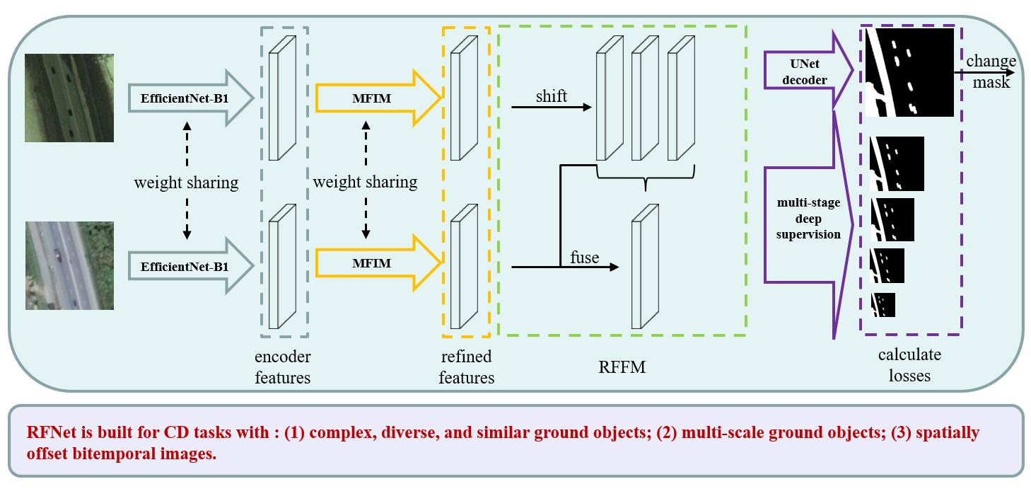
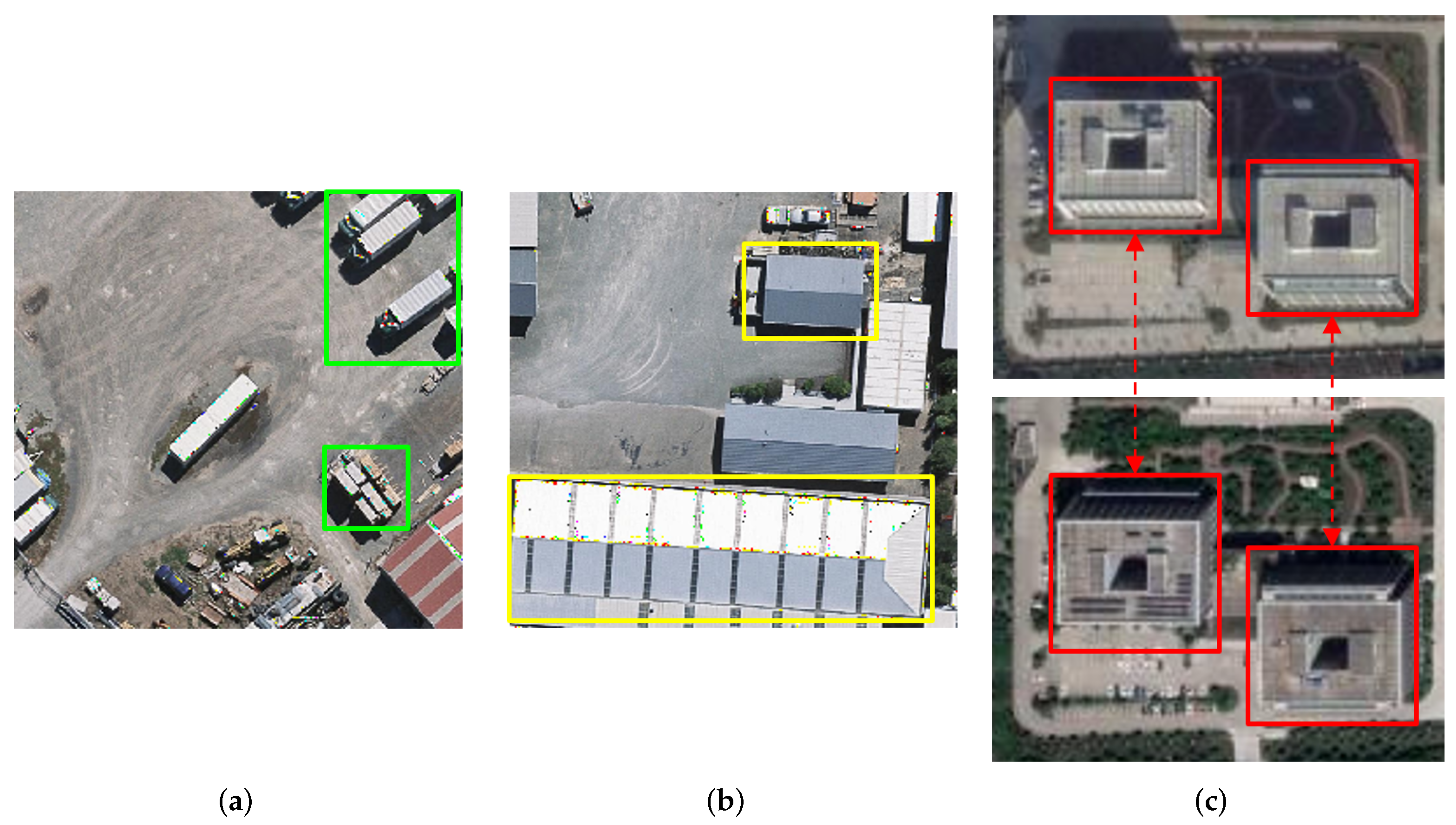
As presented in Figure 1, VHR image CD tasks are still faced with several problems. Firstly, the CD of VHR images is full of complex, diverse, and similar ground objects, making it challenging to extract high discriminative features. However, extracting features with high discrimination can improve the performance of networks. The examples can be found in Figure 1a. Secondly, there exist many ground objects with large scale variations that are sensitive to the resolution of input data. Taking the building CD task as an example, the area of the buildings in Figure 1b varies from tens of pixels to thousands of pixels, which requires the FCNs to identify changes in different stages. Most of the current CD networks extract and fuse multi-stage features hierarchically in the same way as the UNet [62]. Features of each stage only contain information of specific resolution, lacking the interaction of multi-scale features. Finally, there is a lack of CD algorithms that can effectively deal with the spatial offset in bitemporal images. The offset is inevitable as there exist registration errors and different viewing angles between bitemporal images (Figure 1c). The offset usually hinders the optimization of the network and brings pseudo changes to subsequent CD [58]. In the current CD research, few researchers go deep into this issue.
For the sake of solving the above problems, a region-based feature fusion network (RFNet) is designed. The network adopts a common double-stream CD backbone, which inputs bitemporal images to a weight-sharing Siamese encoder and extracts bitemporal features synchronously. The bitemporal features are then enhanced by MFIM and fused by RFFM. The fused features are decoded with a UNet decoder and classified by a naive segmentation head. We can summarize the contributions of this work as follows:
- In the encoding stage, we design MFIM to strengthen the interaction of multi-stage features, so as to better extract features of complex objects and reduce the sensitivity of the network to different scale objects.
- We design RSIM, which takes the neighborhood as the base unit to measure the distance of bitemporal features. The similarity is formulated by introducing prior knowledge to reduce the impact of the spatial offset in bitemporal images.
- Based on RSIM, this paper designs an RFFM to generate changing information by fusing channel-wise enhanced bitemporal features. The RFFM strengthens the learning of change features with few parameters and calculation costs.
- Based on the idea of deep supervision, the region similarities are introduced to auxiliary tasks to help the network directly optimize deep features and get more discriminative features.
We validate the performance of RFNet on two popular CD datasets: the SECOND [63] dataset and the WHU [64] dataset. To prove the feasibility of our proposed modules, comparison experiments between RFNet and several existing state-of-the-art CD architectures are also conducted. We organize the remainder of this paper as follows. Section 2 provides the details of the proposed architecture. Section 3 introduces the two CD datasets. Experimental details and results are discussed in Section 4. We summarize our work and discuss the value, limitations, and future research directions in Section 5.
2. Methodology
This section will provide the details of RFNet. Among them, we first show the overall architecture of RFNet. Then, we introduce the components of the MFIM. Next, the details of RSIM are presented. After that, the architecture of the RFFM is described. In the Section 2.5 we introduce the deep-supervised strategy.
2.1. Overall Structure
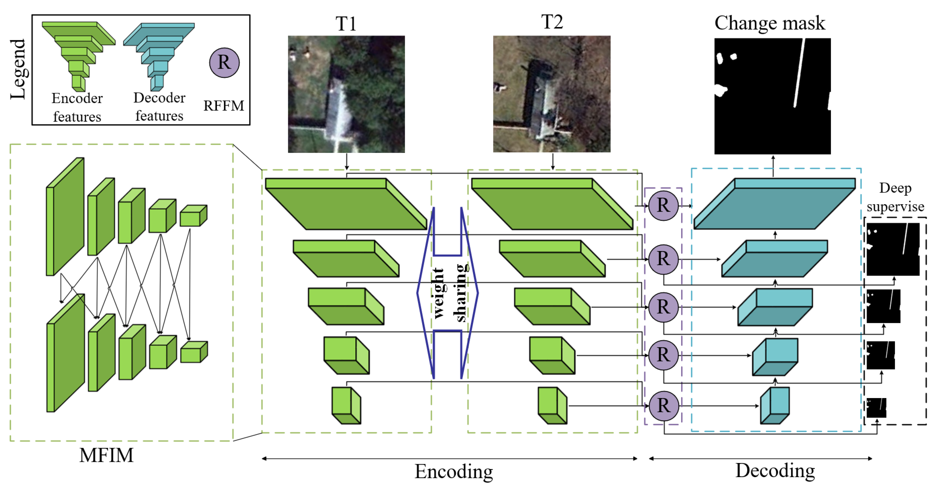
The overall structure of RFNet is shown in Figure 2. To fully exploit the features of ground objects in the VHR images, the two weight-sharing EfficientNet-B1 [65] is used as the dual encoder in the encoding process. Bitemporal images are fed into the weight-shared dual EfficientNet-B1 encoder and generate five-stage encoder features synchronously. Supposing the inputs are bitemporal images with the size of , the outputs of each encoder are five-stage encoder features (with sizes of , , , , and ). The aforementioned encoder features will be input into the MFIM to strengthen the interaction between multi-stage features and obtain the refined encoder features. The illustration of the encoding process is shown in the green rectangles of Figure 2. After obtaining the refined features of bitemporal, the features in the same stage are first fused by a series of RFFM blocks (purple rectangle). Then, fused features are decoded in the same way as skip connections in the UNet decoder. Lower-resolution features are hierarchically upsampled and concatenated with higher-resolution features. Since we use RSIM to measure the similarity of bitemporal features, we directly output RSIM and use the seep supervision strategy to help the network better optimize.
We can formulate RFNet with the following equation:
where and are times downsampled encoder features extracted by the Siamese Efficientnet-B1 encoder. The symbol indicates the MFIM. The MFIM is applied to refine both the pre-temporal features and the post-temporal features in the way of weight-sharing. The symbol represents the RFFM, which is used to fuse refined bitemporal features and generate change features. At last, we use a standard UNet decoder () to decode the change features and output scores for calculating losses.
2.2. Multi-Stage Feature Interaction Module
In the CD tasks of VHR remote sensing images, there are many ground objects with complex appearances and huge scale variations that need multi-scale information to accurately identify changes. Existing CD algorithms mostly obtain changes by fusing the bitemporal features in the same stage. Since features of each stage only contain information of a specific scale, there is often a lack of multi-scale information in the acquisition of change information. So, we propose the MFIM to enhance the interaction of multi-stage features.
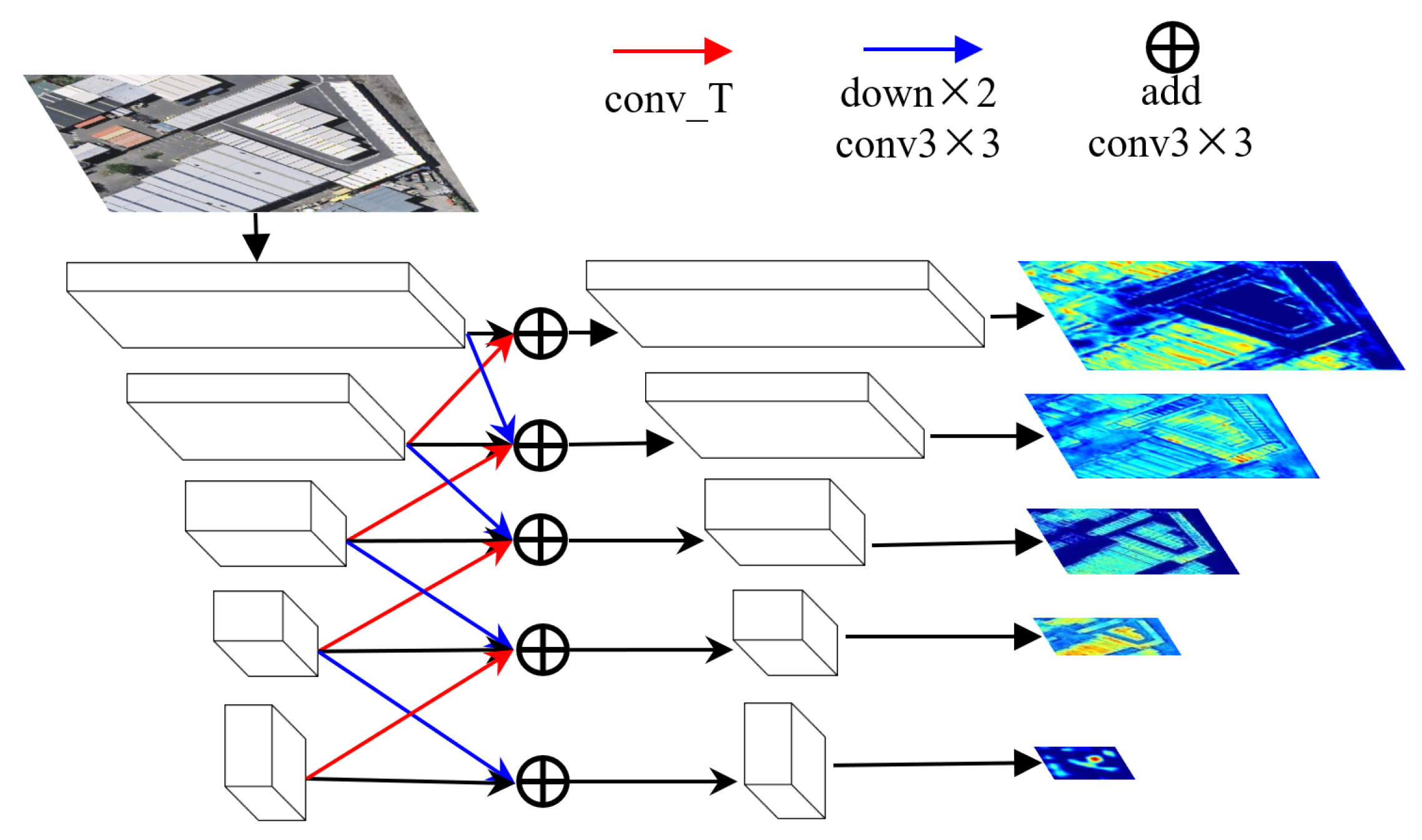
The details of the MFIM are shown in Figure 3. The MFIM is applied to the dual encoder features. The inputs of the MFIM are five encoder features of the same phase. Each input feature will be upsampled or downsampled two times and added with the neighbor features. The outputs of the MFIM are also five features that have the same shape as the input features. The module can be expressed as follows:
where represents the feature of the n-th stage (downsampled times features of bitemporal images), indicates deconvolution with kernel size = 4 and stride = 2, represents max pooling along with a convolution. All the convolutions in and are combined with a batch normalization layer (BN) [66]. The symbol represents the ReLU function. The symbol denotes a convolution combined with BN and ReLU.
2.3. Region Similarity
The spatial consistency of the same ground object between two-period images is critical for the performance of CD algorithms. Unfortunately, in many CD tasks, there exists a large number of spatial offsets between bitemporal ground objects. This kind of shift is often caused by inaccurate image registration and different viewing angles (refer to Figure 1). The spatial offset may hinder the convergence of networks, and sometimes even leads to pseudo changes. Therefore, to address this problem, we design a feature similarity measure based on neighborhood, which takes the neighborhood as the basic unit to calculate the distance between bitemporal features. We name the measure RSIM. RSIM is built to reduce the impact of the spatial offset between bitemporal objects and identify the changes between feature maps more accurately.
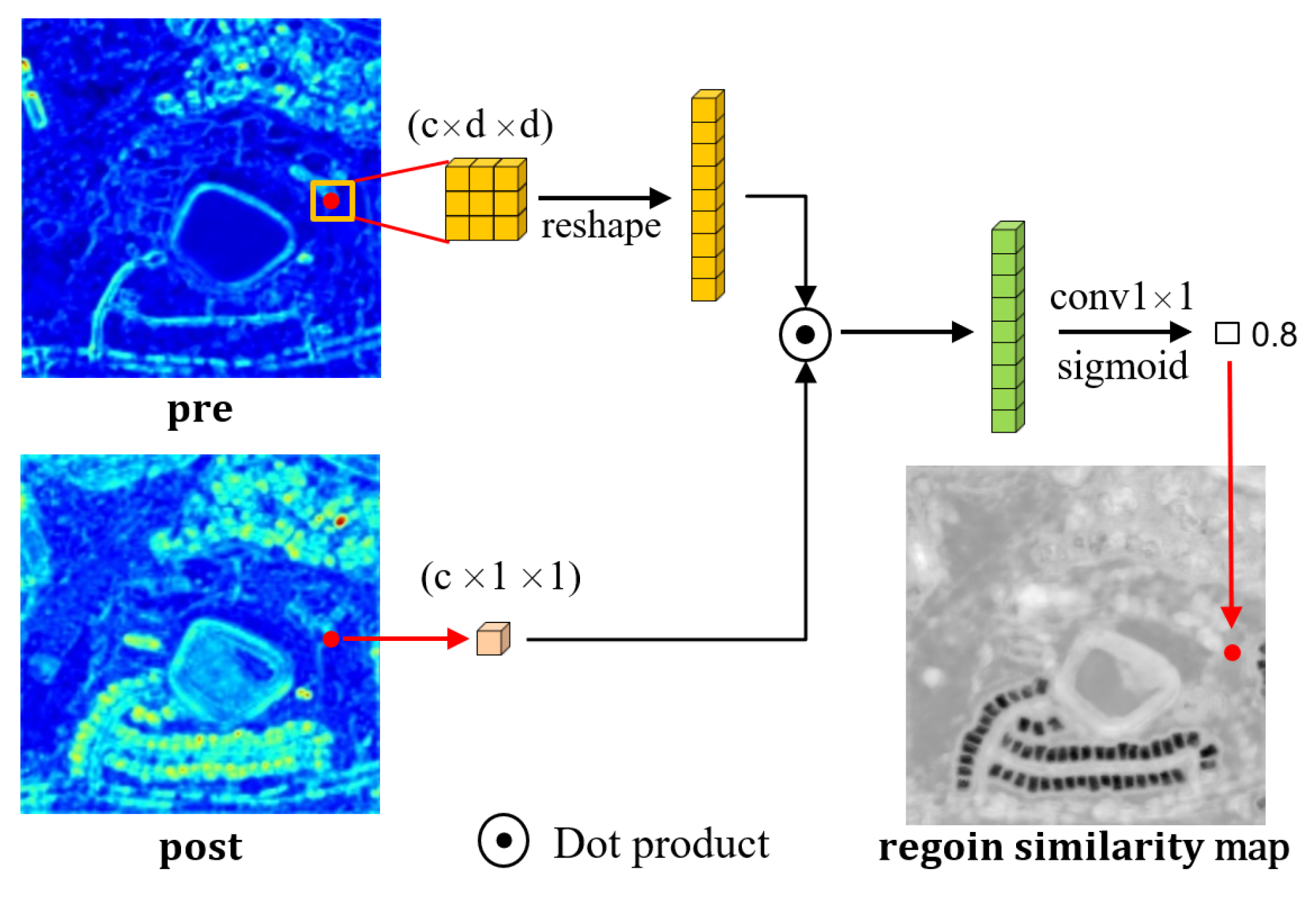
The illustration of RSIM is presented in Figure 4. For bitemporal images and , we have , where H and W denote the height and width of bitemporal images and 3 represents the number of bands. After the encoding stage, the original image is projected to high-dimensional feature space, and we have bitemporal features , where indicates the shape of features. The bitemporal feature vectors of position p can be represented as and . To obtain the RSIM of bitemporal features, we measure the similarity between the feature vector of one phase and the feature vectors in the rectangular region in the other phase. For the position p, we have a rectangular area , where and r is a hyperparameter that represents the radius of the region. The diameter of the region can be calculated as:
Since RSIM measures the similarity between and , the similarity matrix can be represented as and can be calculated with:
where represents the Euclidean distance. For the normalized bitemporal features, can be computed using the dot product:
Hence, in the implementation of the algorithm, we use the () function in Pytorch [67] to generate shifted feature maps and use the matrix multiplication between bitemporal features to calculate the feature similarity:
To get the final similarity map, we input S (in the shape of ) to a convolution layer to reduce the channels by a convolution. After the convolution, a sigmoid function is applied to scale the output and get . Therefore, RSIM can be generated with:
where represents encoder features of one temporal and represented shifted encoder features of the other temporal, v indicates the search range.
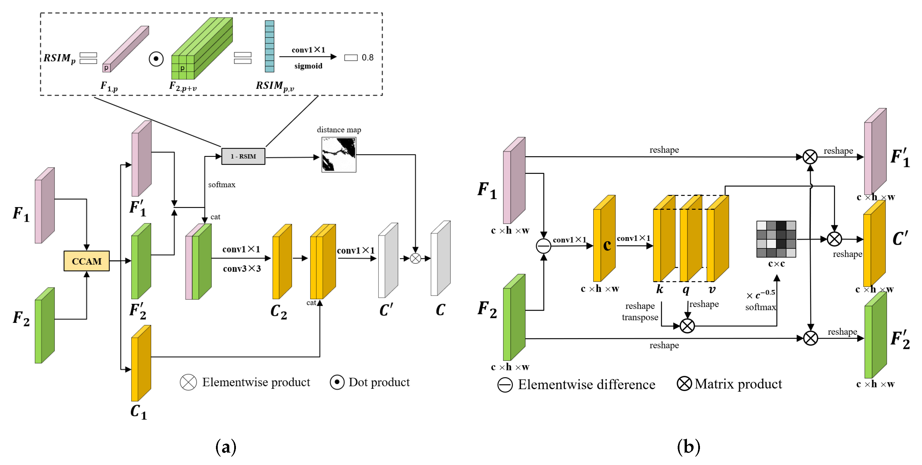
2.4. Region-Based Feature Fusion Module
Based on RSIM, we propose the RFFM to measure the distance of bitemporal features and fuse them to generate change features. The architecture of the RFFM is illustrated in Figure 5a.
Since RSIM mainly measures the similarity in the channel dimension, we first input the bitemporal features into the change channel attention module (CCAM). The CCAM enhances the channels that are correlated to the changes by calculating the correlation between the bitemporal features and the difference feature. More discriminative features can be obtained to better calculate the RSIM. The illustration of the CCAM is shown in Figure 5b. The CCAM is inspired by the channel-wise self-attention module [26,52,68], which obtains the correlation of the channels through the multiplication between the query matrix and the key matrix. The correlated channels are then strengthened by multiplying the value matrix with the correlation map. In the CCAM, we first subtract the bitemporal features and input the result into a convolution to get the difference feature :
where and are the bitemporal features. After that, we use a convolution to expand the channels and split them into the query matrix (k), query matrix (q), and value matrix (v):
According to the calculation self-attention map, we first reshape k, q, and v from to and we have . The correlation map can be calculated with:
where · denotes the matrix multiplication, T represents the transpose operation, and is the correlation map with the shape of . represents the importance of the channels to the change information extraction. We use to strengthen the correlated channel of bitemporal features and change features. The outputs of the CCAM are formulated as:
A coarse change feature () and reweighted bitemporal features ( and ) are the outputs of the CCAM. The feature and are concatenated and processed by convolution layers to generate another coarse change feature :
We then concatenate and and process them with a convolution to get a fine change feature ():
Simultaneously, based on RSIM, the distance (D) between and is generated with:
where r represents the radius of the search region, . Then, and D are then multiplied so that pseudo changes are suppressed and change features are emphasized:
To sum up, the RFFM can be expressed as:
where represents the CCAM, and and are bitemporal refined encoder features generated with MFIM. The symbol C indicates the change feature, which will be fed into a standard UNet decoder. After the processing of RFFM, change features from different stages are hierarchically decoded by a simple UNet decoder and classified by a common segmentation head. The change features generated by the RFFM can be considered to be skip connections.
In this paper, four RFFMs are used to fuse the second to fifth stage bitemporal features respectively, and the neighborhood radius is set to 2. For the features of the first stage, because the shallow features lack semantic information, we fuse them with a simple concatenation followed by a convolution. Since the RFFM introduces RSIM to strengthen the learning of change features, it can help the network better deal with the spatially offset ground objects. At the same time, by introducing prior knowledge into the calculation of change information, the RFFM can help obtain change information with a few parameters and calculation costs.
2.5. Deep Supervise-Based Loss Function
We choose the Dice coefficient as the main loss of this work. The loss function is formulated as:
The symbol C denotes the confidence output of the network, L represents the label, and ∩ denotes the intersection of C and L.
Introducing intermediate layers into the loss functions can shorten the error propagation distance and boost the performance of the network [53,59,61]. Therefore, we formulate a deep supervised strategy by directly introducing the RSIM to the calculation of losses. Since and is normalized with sigmoid function, for each pixel in position i, we have . We directly supervise the learning of RSIM by constraining the average value in both the changing regions and the non-changing regions. For the features in the changing regions, we hope that the smaller the RSIM is, the better, while for the unchanged area, we hope that the larger the RSIM is, the better. To ensure the deep-supervised loss is within a reasonable range, we use the logarithm of the mean value as the output and the loss can be calculated as:
where indicates the ground truth and we have of , indicates natural logarithm. As presented in Section 2.4, the RFFM is not applied to fuse the first-stage bitemporal features. Therefore, the overall loss of RFNet can be calculated with:
where the value 2 and 5 represent the second to the fifth stage features.
3. Datasets
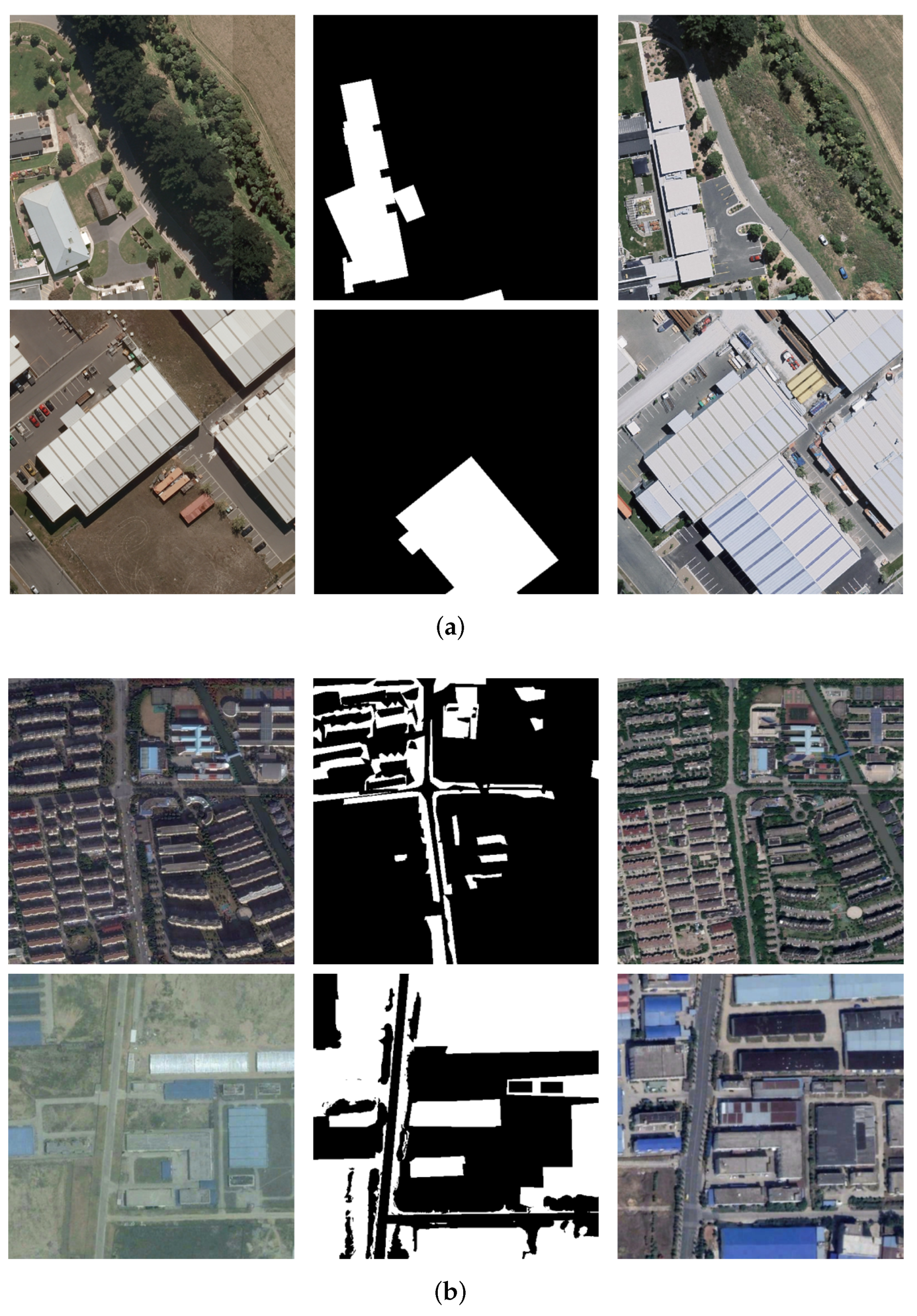
We verify the feasibility of RFNet through two public CD datasets: WHU and SECOND. Some examples of the experimental datasets are presented in Figure 6.
3.1. SECOND dataset
The SECOND dataset is built with 2968 pairs of samples. The image resolution ranges from 3 m to 0.5 m. The dataset is built to detect several land cover changes. We randomly split the samples into train/validation/test sets based on a ratio of 6:2:2.
For the SECOND dataset, we plot representative samples in Figure 6b. As is shown in the examples, the SECOND dataset is a changeling dataset with the spatial offset of the buildings and the radiation difference of background objects. Therefore, we choose this dataset as the experimental dataset.
3.2. WHU Dataset
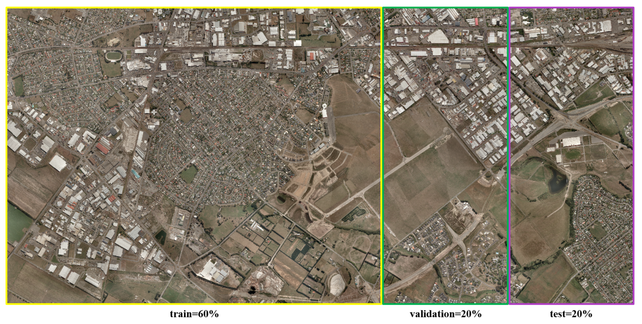
The WHU dataset is aimed at detecting building changes with a pair of RGB data. The dataset consists of two VHR images (0.3 m) and the size of the images is 32,507 × 15,354. The dataset contains over 12,796 buildings in the pre-temporal image and contains 160,77 buildings in the post-temporal image. We build the train/validation/test sets by splitting the samples based on a ratio of 6:2:2. Every two sets are spatially separated. The details of the splitting strategy are shown in Figure 7. For each set, we crop the bitemporal images and the change mask into chips. For the slices of the training set, we use an additional overlap strategy, which keeps a 256 overlap on both the horizontal side and the vertical side.
Several examples of the WHU dataset can be found in Figure 6a. From the example of the WHU dataset, we can learn that there are a lot of buildings with large scale variations and many background objects similar to buildings. To this end, we use this dataset to validate the capability of our work.
4. Experiments and Results
This subsection will discuss our implementation settings and experimental results in detail. We first introduce our benchmark methods, then we provide our implementation details, and finally, we present the qualitative and quantitative comparison results.
4.1. Benchmark Methods
The benchmark methods we use are recently proposed DL-based CD architectures. A brief introduction to the benchmark methods is as follows.
- FC-EF [51]: A fully convolution early fusion CD network that inputs channel-wise stacked bitemporal images and outputs change masks. The network generates change masks in an encode–decode manner.
- FC-Siam-Conc [51]: A fully convolutional siamese-concatenation CD network. This is a Siamese network that separates the encoding layers of FC-EF into dual streams with weight sharing. Bitemporal images are fed into the dual streams and generate bitemporal features. The bitemporal features are directly sent to the decoder and fused with concatenation.
- FC-Siam-Diff [51]: A fully convolutional Siamese-difference network for CD tasks. Different from FC-Siam-Conc, it decodes the difference of dual encoder features to gain the change mask.
- CDNet [39]: CDNet is a UNet-like CD network, which inputs concatenated bitemporal images. All the convolution layers are designed with kernel size = 7.
- UNet++_MSOF [11]: The network first concatenates bitemporal images to multi-spectral data and inputs it to a modified UNet++ network. Features from different semantic stages of UNet++ are fused to get the final change maps.
- IFN [59]: IFN is a fully convolutional Siamese CD network that introduces deep supervision into CD tasks. The network uses spatial-wise and channel-wise attention modules to fuse multi-level deep features. To help better optimize the network and enhance network performance, a deep supervision strategy is introduced in the intermediate features.
- SNUNet_CD [60]: A CD network built with dense connections. The network is made up of a dual UNet encoder and a UNet++ decoder. The channel-wise attention mechanism is introduced in deep supervision and an ensemble channel-wise attention module is proposed to refine representative features of different semantic levels for the final classification.
- BiT [69]: The network introduces a vision transformer into CD tasks. Bitemporal images are embedded into tokens and are fed to the transformer module to generate context information in the compact token-based space-time.
As in most CD tasks, the number of changed pixels and unchanged pixels is often seriously imbalanced. Therefore, metrics such as overall accuracy are often insensitive to the changed regions and lead to results with dominant predictions of non-change pixels getting unreasonable better accuracy [63]. So, to make a better evaluation, the F1-score (F1) and intersection over union (IoU) are chosen as indicators of different architectures. Both aforementioned metrics can relieve the influence of imbalanced labels. To better evaluate the models’ ability to reduce pseudo changes and missing changes, recall and precision are also chosen as the evaluation matrix. To avoid the unfair comparison caused by more model parameters, we also take the parameters of the model (Params) as a main evaluating indicator.
4.2. Training Details
RFNet and all the benchmark methods are implemented with the Pytorch DL framework. We train all the models on two RTX 3090 GPUs (24 GB memory). In the training process, the minibatch size of RFNet is 12 on each GPU. We choose AdamW [70] as the optimizer and Dice (Formula (17)) as the main loss of all the networks. The initial learning rate is 0.002 and is adjusted by an exponential learning rate strategy. In each epoch during training, the learning rate can be calculated by the following formula:
where represents the initial learning rate, is a constant factor and is set to 0.96, is the current epoch index, and the maximum of the is set to 150.
To enrich the diversity of training samples, we adopt several data augmentation strategies. The augmentation functions include (1) randomly scaling the images with a scale factor set to 0.1; (2) randomly flipping and transposing; (3) randomly rotating 90°, 180°, and 270°; (4) randomly HSV shift with the range set to 20; (5) randomly switch the phase of bitemporal images; (6) randomly add Gaussian noise with the mean value set to 0 and variance ranges from 10 to 50. All the data augmentation functions are applied with a probability of 0.5.
4.3. Ablation Study
The ablation study is conducted in this part to prove the improvement and effectiveness of our proposed architectures. All the experiments in the ablation study are implemented with the same details presented in Section 4.2. In the ablation study, the proposed modules are applied to the baseline to show performance improvement. The baseline is a simple Siamese network, which is constructed by the combination of a Siamese Efficientnet encoder and a UNet decoder. In the baseline, bitemporal encoder features are fused with concatenation and a convolution layer. We mainly use IoU, F1, and Params as indicators for comparison. To reduce the influence of random error in training, we train each model three times and fill the average IoU and F1 into the table.
4.3.1. Comparison of MFIM
We first compare the performance improvement of MFIM by adding MFIM to the baseline. As a comparison experiment, we also test the baseline on the two datasets and present the performance in the first row of Table 1. In the second row, we fill the table with the indicators generated by applying MFIM to the baseline. As the values shown in the table, MFIM can remarkably improve the baseline’s performance on both datasets. With the interaction of multi-stage features, the network can better extract features of complex objects. On the SECOND dataset, MFIM improves 1.62% in IoU and 1.35% in F1. Although the baseline scores a better recall (72.37%), its precision (67.94%) is much lower than the combination of baseline and MFIM, which means it introduces many pseudo changes in the results. On the WHU dataset, both precision and recall are improved, which means more building changes with better internal compactness are detected.
We also present a visual comparison in Figure 8. We plot the inference results of the SECOND dataset in Figure 8a and the inference results of the WHU dataset in Figure 8b. From the figure, we can conclude that MFIM can effectively identify changes with different scales and similar appearances. In the first two rows of Figure 8a, there are large scale changes in the bitemporal images. The baseline detects changes in the wrong scale and performs broken results, while the baseline with the MFIM presents better internal compactness in the change masks. In the third row of Figure 8a, many buildings of different sizes require the network to extract building features in different scales. In the center of the result, the baseline with the MFIM finds two small building changes that are missed by the naive baseline. The abovementioned situation also happens in the first two rows of Figure 8b. From the last row of Figure 8a, we can learn that introducing MFIM to the baseline can better distinguish the low vegetation surface from the non-vegetated ground surface so that more complete changes can be found. In the last two rows of Figure 8b, there are pseudo changes in the outputs of the baseline. These changes can be effectively filtered out by introducing multi-scale information into the feature extraction process.
4.3.2. Comparison of RFFM
To validate the applicability of the RFFM, we conduct an ablation study in this subsection. We present the performance of the baseline with/without the RFFM in Table 2. The values in the table show that when the RFFM is adopted, both the IoU and F1 can be increased. The better performance mainly comes from the significant improvement in precision (4.96% on SECOND and 2.21% on WHU), which means the RFFM can effectively reduce the impact of the spatial offset in bitemporal images and filter out pseudo changes. It should be noted that introducing RFFM only costs 0.2 Mb extra parameter.
We can also observe the applicability of the RFFM by the inference results in Figure 9. The first row of Figure 9a and the first two rows of Figure 9b illustrate that the baseline has lower robustness to the radiation difference between bitemporal images, which results in false positives in the baseline’s output. By introducing the RFFM into the baseline, these background changes can be reduced effectively. In the second to the fourth row of Figure 9a, there are spatial biases in bitemporal buildings that cause pseudo changes in the baseline. Compared with the simple baseline, the combination of the baseline and the RFFM can better deal with spatial misalignment and reduce false detections. The last two rows of Figure 9b demonstrate the robustness of the RFFM to the building shadows. The outputs of the baseline with the RFFM show fewer pseudo changes when the buildings hide in shadows.
4.3.3. Comparison of Deep Supervision
We conduct comparison experiments on adopting deep supervision. Since the deep supervised strategy can only be used with the RFFM applied, we compare the performance of deep supervision based on the combination of baseline and the RFFM. The comparison results are shown in Table 3. By observing the table, we can learn that using deep supervised loss can further improve the performance with no additional parameter cost. Although the precision reduced slightly on both datasets, the recall can be significantly improved. We can attribute this improvement to the learning of more discriminative features. Changing features are well separated from unchanging ones, so small changes can be better detected.
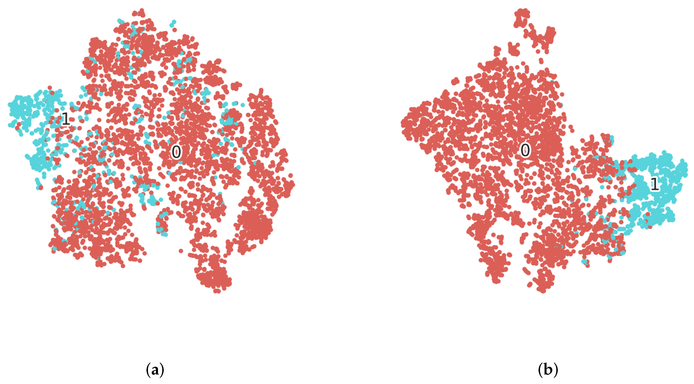
To better prove that using deep supervision can learn more discriminative features, we also visualize the features without and with deep supervision in Figure 10. The features are visualized with t-SNE [71], a dimension reduction algorithm that can project high-dimensional features onto a two-dimensional plane. From the figure, we can learn that features with deep supervision are more distinguishable. Both changed features and unchanged features are well grouped.
4.4. Comparisons on SECOND
We compare RFNet and all the benchmark methods on the SECOND dataset and discuss the comparison results in this subsection. The performance of different architectures is presented in Table 4. From the table, we can conclude that among all the testing algorithms, RFNet achieves the best IoU and F1 with a relatively low parameter cost. Although models such as FC-EF and FC-Sima-diff have the fewest parameters, their scores are much lower than other methods. IFN, SNUNet_CD, and BiT have larger parameter quantities than RFNet, but RFNet still outperforms these comparison methods with at least 1.3% in IoU and 1% in F1.
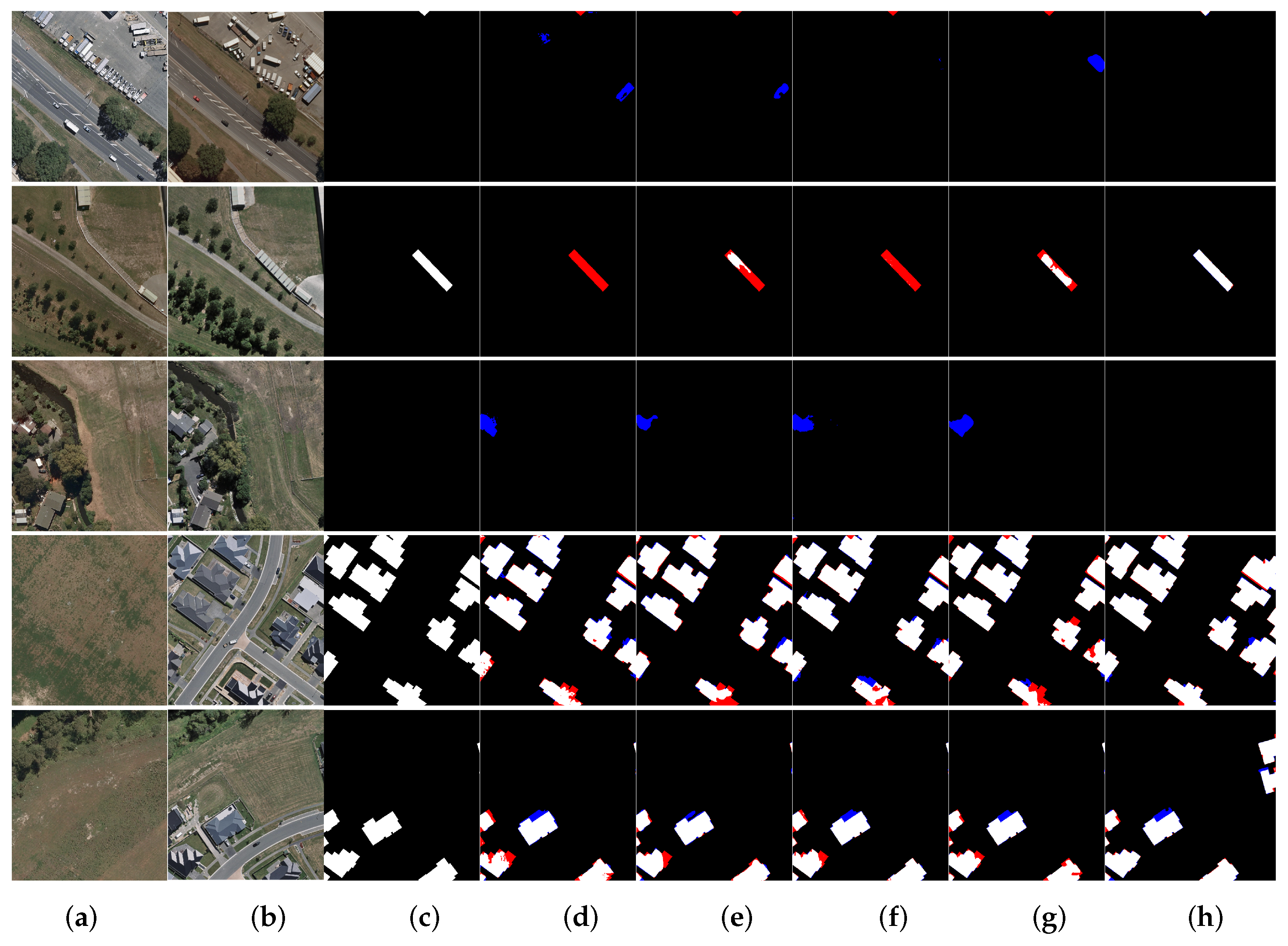
Figure 11 shows a visual comparison of the top five CD models on SECOND, including FC-Sima-diff, IFN, SNUNet_CD, BiT, and RFNet. As illustrated by the figure, RFNet has an obvious advantage over other networks in accuracy. As is shown in the second and fourth rows, RFNet performs the best internal integrity for changes with a large scale variation. In the third and fifth rows, there exist buildings that are spatially biased in bitemporal images. Under this circumstance, the results of RFNet contain the fewest pseudo changes among all the testing methods. At the center of the second row, there exists a building change, and the change is not labeled in the ground truth. All the comparison methods can identify the change mentioned before, but the result of RFNet attains the best boundary accuracy. At the bottom of the third row, all the inference results miss the change in the building. This is understandable because many changes in building appearance are not labeled.
4.5. Comparison on WHU
We also conduct comparison experiments on the WHU dataset. The quantitative comparison is shown in Table 5. By analyzing the table, we can learn that RFNet achieves the best performance in both IoU (86.02%) and F1 (92.49%). Compared with the benchmark methods, RFNet has improved by at least 3.5% in IoU and 2% in F1. Owing to introducing multi-scale information and using neighborhood information for differing, RFNet gains the best precision (95.72%) and the second-best recall (89.46%), which means RFNet can accurately find the changes in bitemporal images.
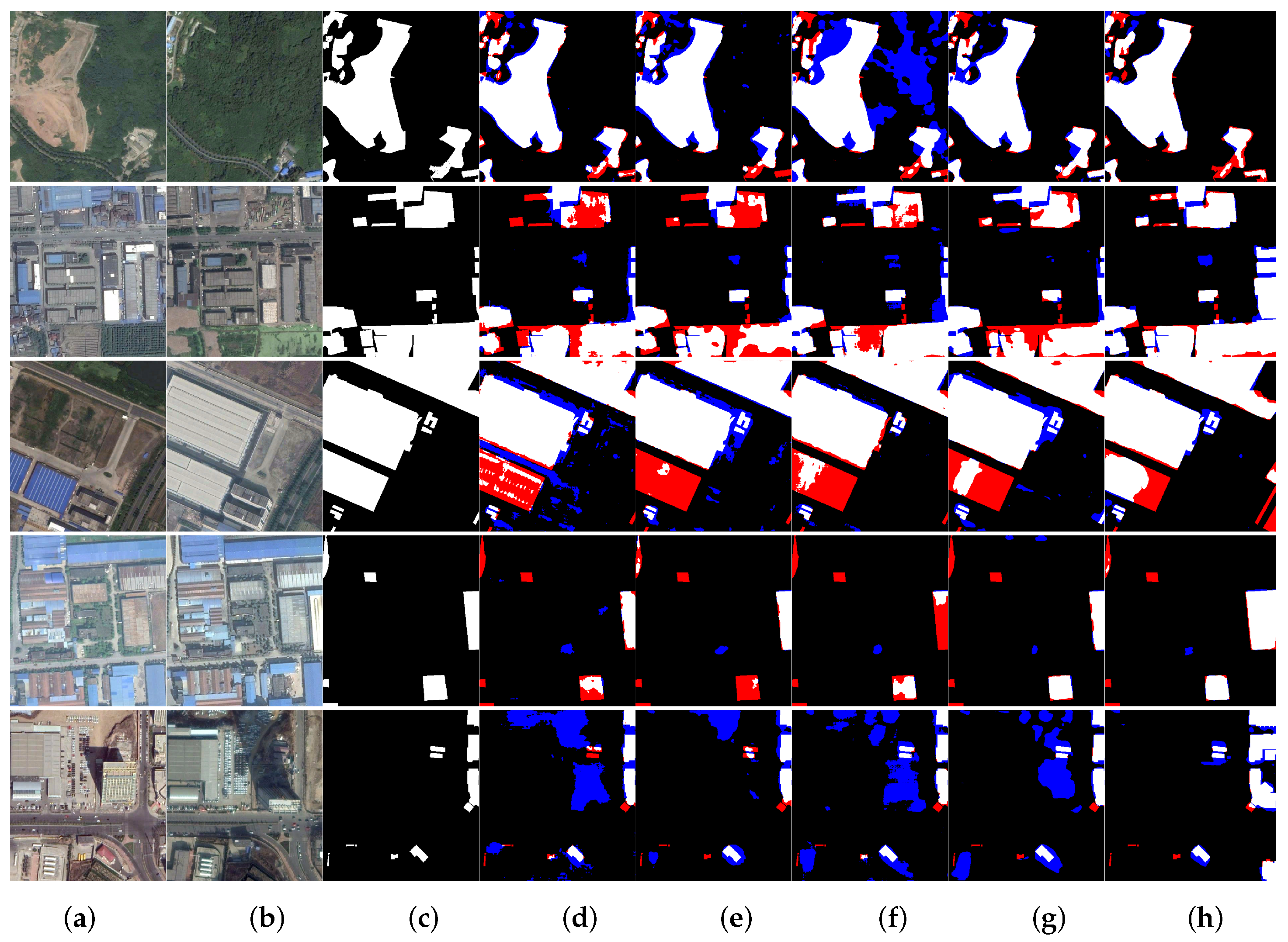
To show the performance more intuitively, we visualize the results of RFNet and benchmark methods in Figure 12. We plot the results of FC-Sima-diff, IFN, SNUNet_CD, BiT, and RFNet as they are still the top five best models on the WHU dataset. As shown from the figure, RFNet attains the best visual performance among all the testing methods with fewer pseudo changes and fewer missed detections. From the first two rows, we can learn that RFNet can better distinguish buildings from other background objects. In the third row, RFNet can avoid false detections when buildings in the pre-temporal image are covered by trees. Results in the last two rows can demonstrate that RFNet performs well in maintaining the integrity of the buildings and detecting accurate building boundaries.
4.6. Robustness Experiments
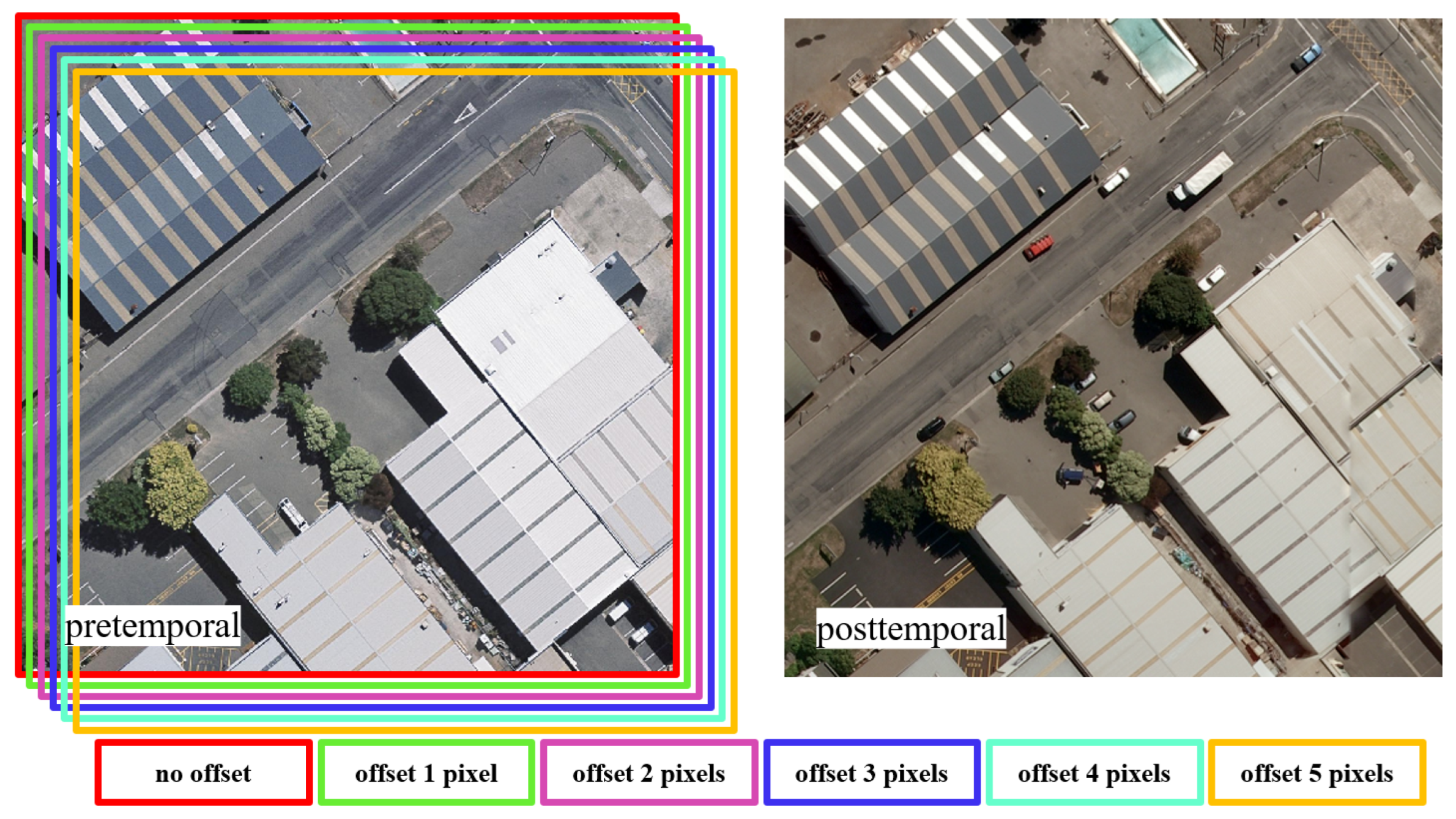
Since the change discrimination module used in this paper is partially built with prior knowledge, rather than learning, the integration of physics models and machine learning architectures may improve the models’ performance and generalization ability [24]. Theoretically speaking, the method in this paper is more robust to bitemporal images with spatial offset. Therefore, to prove the robustness of RFNet to the spatially shifted bitemporal images, we carry out comparative experiments on bitemporal data with different migration degrees. We conduct robustness tests on both the SECOND dataset and the WHU dataset. The way we shift bitemporal images is shown in Figure 13. We use the function in Pytorch to realize the offset of bitemporal images with the corresponding number of pixels.
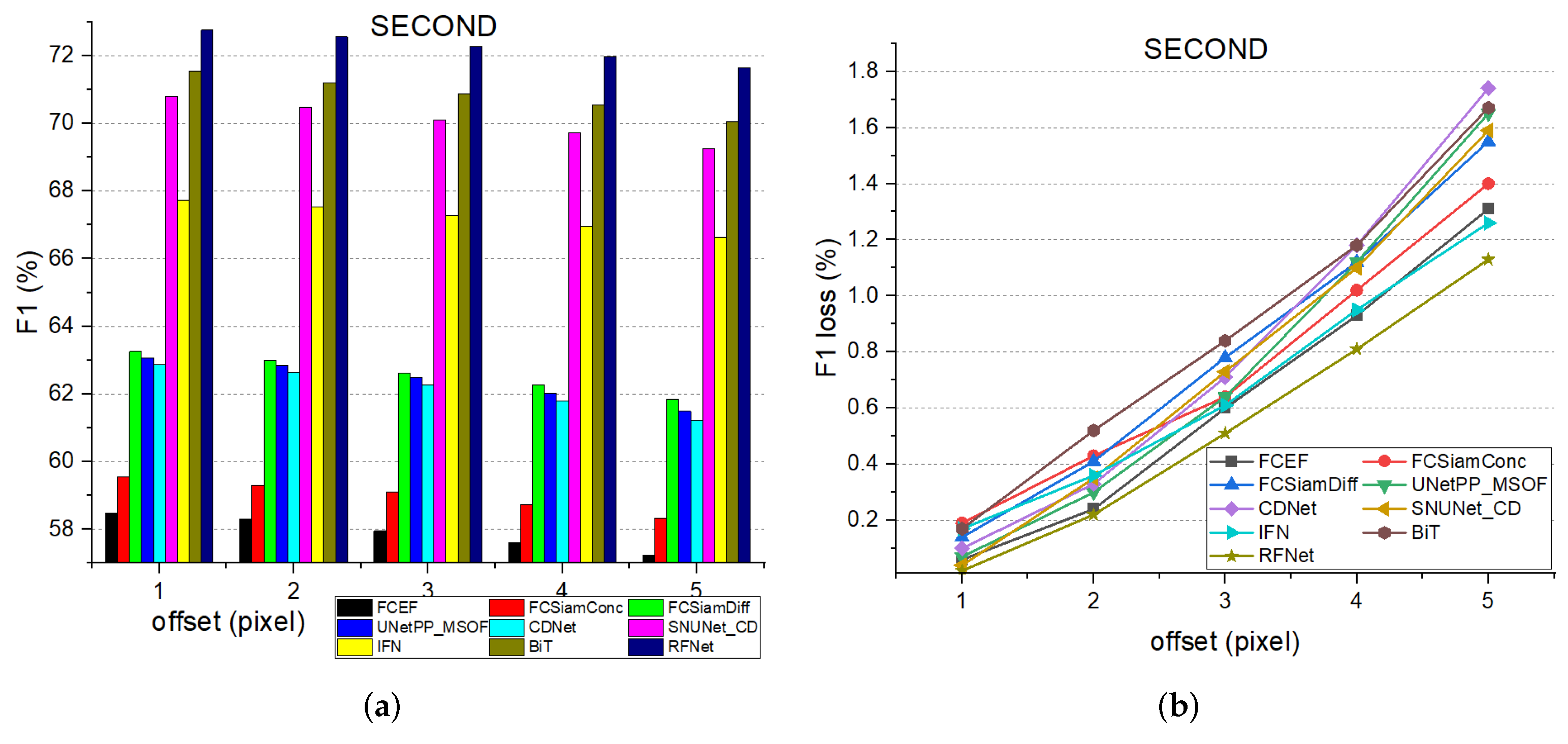
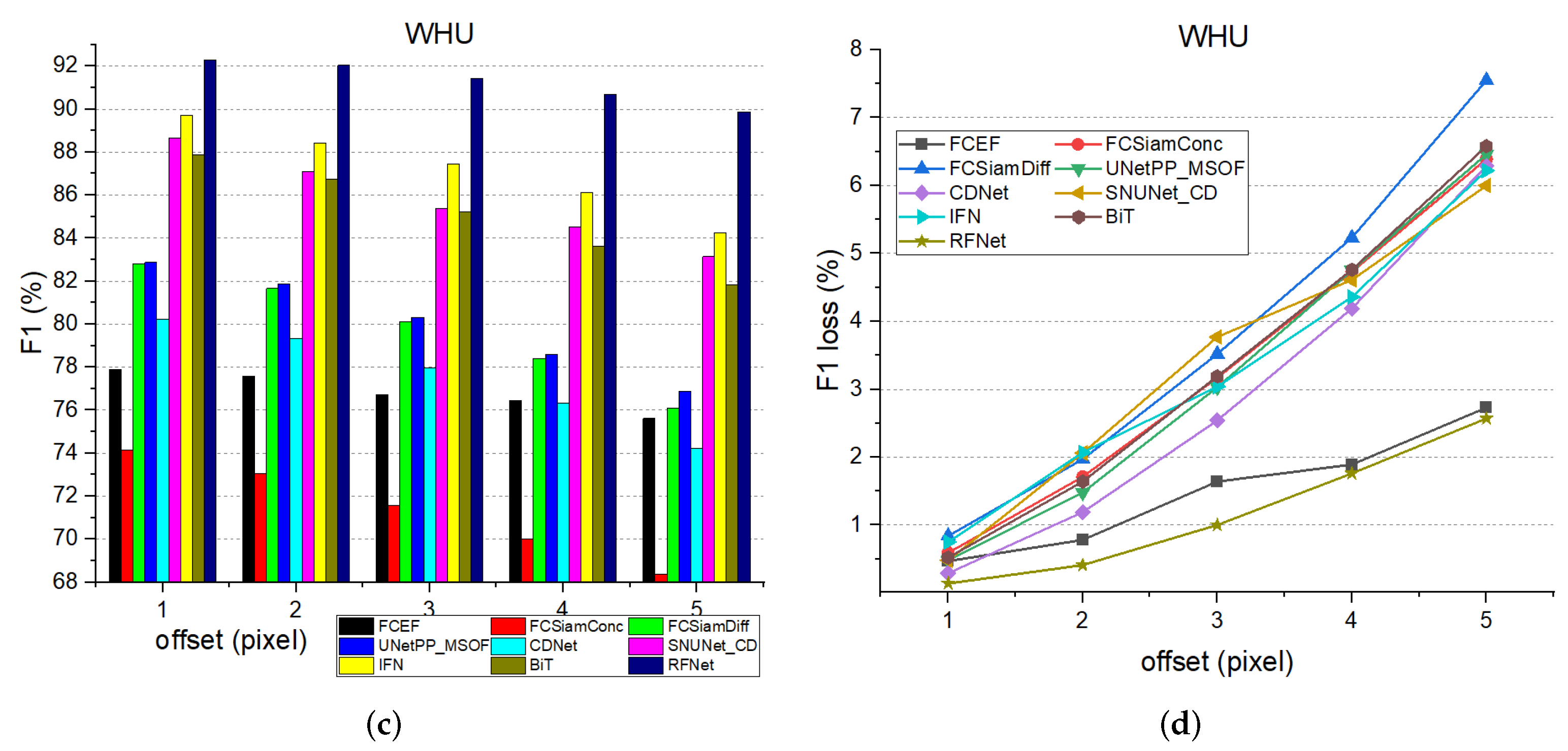
The experimental results are shown in Figure 14. To better show the robustness of all the testing architectures, we plot both the F1 and the loss of F1 corresponding to the different number of shifting degrees. The number of shifting pixels ranges from 1 to 5. From the figure, we can learn that RFNet has a strong robustness to the spatially misaligned bitemporal images. On the SECOND dataset, there is a loss of 1.13% in F1 when the pre-temporal images are shifted by 5 pixels, which is the least loss among all the networks. On the WHU dataset, RFNet only loses 2.57% in F1 when offset by 5 pixels, which is much lower than most methods.
5. Conclusions
This paper designs a region-based feature fusion model for CD tasks. The model uses the MFIM to facilitate the interaction of multi-scale features and uses the RFFM to fuse bitemporal features by considering features in the neighborhood. The modules presented in this paper are evaluated by two popular change detection datasets: the SECOND dataset and the WHU dataset. The experiments prove that the proposed method has certain advantages over the existing methods. Compared with the baseline and all the benchmark architectures, the proposed model achieves better performance with a small parameter overhead.
This paper can also be regarded as an attempt to integrate DL architectures with physics models. With the development of DL-based algorithms and the accumulation of remote sensing data, we can better observe the ground surface based on powerful interpretation tools. Although DL algorithms (data-driven) have stronger feature extraction ability and more powerful modeling capability than traditional algorithms (theory-driven), there are still two inherent problems. For one thing, the optimization of DL models is often completely dependent on the training samples, which will cause cognitive loss. It is difficult to understand the knowledge learned by DL models, and it is also difficult for us to require the model to learn what we want. Secondly, data-driven algorithms learn the distribution of features based on the training samples. When testing the model on an unseen dataset with a large difference in data distribution from the training data, the model performance is often poor. In contrast, traditional physical modeling methods often go through strict assumptions and complex modeling and are more universal for the studies. Therefore, integrating the physical model theory and the powerful learning ability of DL has become a challenge. To tackle the abovementioned challenge, this research makes some attempts in the field of CD. By introducing prior knowledge to distinguish the changes in the DL features, the algorithm achieves higher accuracy and better robustness to spatially offset bitemporal images.
Although RFNet shows high accuracy and strong robustness to VHR image CD tasks, it is still faced with several limitations. For the proposed network architecture, the efficiency of RFNet could be improved. As RSIM takes features in the neighborhood into the calculation, the inference of RFNet is not very efficient. Fortunately, during the training process, RSIM does not participate in backpropagation, which means the RFFM is not a time-consuming module while training. For the performance of RFNet, the network’s outputs are still not accurate enough. For example, there are many misdetections on the SECOND dataset between low-vegetated and non-vegetated surfaces. These changes are hard to identify both with DL architectures and human eyes. To further improve the model’s performance to complex ground objects, multi/hyper-spectral data need to be applied. For the training of RFNet, a large number of well-labeled samples are required to train the network. However, building a CD dataset is extremely time-consuming in most CD tasks.
Future work will focus on four aspects: (1) incorporating more machine learning models and physical models; (2) speeding up model processing; (3) introducing multi/hyper-spectral data in CD tasks; (4) researching semi-supervised and weakly supervised CD algorithms.
Author Contributions
Conceptualization, P.C. and B.Z.; methodology, P.C. and C.L.; software, P.C. and Z.C.; validation, P.C., X.Y. and K.L.; formal analysis, P.C. and L.Z.; investigation, C.L.; resources, P.C.; data curation, P.C. and Z.C.; writing—original draft preparation, P.C. and L.Z.; writing—review and editing, B.Z. and L.Z.; visualization, P.C.; supervision, Z.C.; project administration, B.Z.; funding acquisition, Z.C. All authors have read and agreed to the published version of the manuscript.
Funding
The work was supported by the National Key Research and Development Program of China (Grant No.2021YFB3901202) and the National Natural Science Foundation of China (Grant No. 42071407).
Data Availability Statement
Not applicable.
Acknowledgments
The authors thank the editors and anonymous reviewers for their valuable comments, which greatly improved the quality of the paper.
Conflicts of Interest
The authors declare no conflict of interest.
References
- Singh, A. Review article digital change detection techniques using remotely-sensed data. Int. J. Remote Sens. 1989, 10, 989–1003. [Google Scholar] [CrossRef] [Green Version]
- Hussain, M.; Chen, D.; Cheng, A.; Wei, H.; Stanley, D. Change detection from remotely sensed images: From pixel-based to object-based approaches. ISPRS J. Photogramm. Remote Sens. 2013, 80, 91–106. [Google Scholar] [CrossRef]
- Quarmby, N.; Cushnie, J. Monitoring urban land cover changes at the urban fringe from SPOT HRV imagery in south-east England. Int. J. Remote Sens. 1989, 10, 953–963. [Google Scholar] [CrossRef]
- Howarth, P.J.; Wickware, G.M. Procedures for change detection using Landsat digital data. Int. J. Remote Sens. 1981, 2, 277–291. [Google Scholar] [CrossRef]
- Richards, J. Thematic mapping from multitemporal image data using the principal components transformation. Remote Sens. Environ. 1984, 16, 35–46. [Google Scholar] [CrossRef]
- Jin, S.; Sader, S.A. Comparison of time series tasseled cap wetness and the normalized difference moisture index in detecting forest disturbances. Remote Sens. Environ. 2005, 94, 364–372. [Google Scholar] [CrossRef]
- Xing, J.; Sieber, R.; Caelli, T. A scale-invariant change detection method for land use/cover change research. ISPRS J. Photogramm. Remote Sens. 2018, 141, 252–264. [Google Scholar] [CrossRef]
- Zerrouki, N.; Harrou, F.; Sun, Y.; Hocini, L. A machine learning-based approach for land cover change detection using remote sensing and radiometric measurements. IEEE Sens. J. 2019, 19, 5843–5850. [Google Scholar] [CrossRef] [Green Version]
- Ma, W.; Wu, Y.; Gong, M.; Xiong, Y.; Yang, H.; Hu, T. Change detection in SAR images based on matrix factorisation and a Bayes classifier. Int. J. Remote Sens. 2019, 40, 1066–1091. [Google Scholar] [CrossRef]
- Fisher, P. The pixel: A snare and a delusion. Int. J. Remote Sens. 1997, 18, 679–685. [Google Scholar] [CrossRef]
- Peng, D.; Zhang, Y.; Guan, H. End-to-end change detection for high resolution satellite images using improved UNet++. Remote Sens. 2019, 11, 1382. [Google Scholar] [CrossRef] [Green Version]
- Addink, E.A.; Van Coillie, F.M.; De Jong, S.M. Introduction to the GEOBIA 2010 special issue: From pixels to geographic objects in remote sensing image analysis. Int. J. Appl. Earth Obs. Geoinf. 2012, 15, 1–6. [Google Scholar] [CrossRef]
- Lefebvre, A.; Corpetti, T.; Hubert-Moy, L. Object-oriented approach and texture analysis for change detection in very high resolution images. In Proceedings of the IGARSS 2008-2008 IEEE International Geoscience and Remote Sensing Symposium, Boston, MA, USA, 7–11 July 2008; Volume 4. [Google Scholar]
- De Chant, T.; Kelly, M. Individual object change detection for monitoring the impact of a forest pathogen on a hardwood forest. Photogramm. Eng. Remote Sens. 2009, 75, 1005–1013. [Google Scholar] [CrossRef] [Green Version]
- Dingle Robertson, L.; King, D.J. Comparison of pixel-and object-based classification in land cover change mapping. Int. J. Remote Sens. 2011, 32, 1505–1529. [Google Scholar] [CrossRef]
- El Amin, A.M.; Liu, Q.; Wang, Y. Zoom out CNNs features for optical remote sensing change detection. In Proceedings of the 2017 2nd International Conference on Image, Vision and Computing (ICIVC), Chengdu, China, 2–4 June 2017; pp. 812–817. [Google Scholar]
- Zheng, Z.; Wan, Y.; Zhang, Y.; Xiang, S.; Peng, D.; Zhang, B. CLNet: Cross-layer convolutional neural network for change detection in optical remote sensing imagery. ISPRS J. Photogramm. Remote Sens. 2021, 175, 247–267. [Google Scholar] [CrossRef]
- Hou, X.; Bai, Y.; Li, Y.; Shang, C.; Shen, Q. High-resolution triplet network with dynamic multiscale feature for change detection on satellite images. ISPRS J. Photogramm. Remote Sens. 2021, 177, 103–115. [Google Scholar] [CrossRef]
- Peng, X.; Zhong, R.; Li, Z.; Li, Q. Optical Remote Sensing Image Change Detection Based on Attention Mechanism and Image Difference. IEEE Trans. Geosci. Remote. Sens. 2020, 59, 7296–7307. [Google Scholar] [CrossRef]
- Shafique, A.; Cao, G.; Khan, Z.; Asad, M.; Aslam, M. Deep learning-based change detection in remote sensing images: A review. Remote Sens. 2022, 14, 871. [Google Scholar] [CrossRef]
- Zhang, Y.; Fu, L.; Li, Y.; Zhang, Y. HDFNet: Hierarchical Dynamic Fusion Network for Change Detection in Optical Aerial Images. Remote Sens. 2021, 13, 1440. [Google Scholar] [CrossRef]
- Cheng, H.; Wu, H.; Zheng, J.; Qi, K.; Liu, W. A hierarchical self-attention augmented Laplacian pyramid expanding network for change detection in high-resolution remote sensing images. ISPRS J. Photogramm. Remote Sens. 2021, 182, 52–66. [Google Scholar] [CrossRef]
- Zhang, B.; Chen, Z.; Peng, D.; Benediktsson, J.A.; Liu, B.; Zou, L.; Li, J.; Plaza, A. Remotely sensed big data: Evolution in model development for information extraction [point of view]. Proc. IEEE 2019, 107, 2294–2301. [Google Scholar] [CrossRef]
- Reichstein, M.; Camps-Valls, G.; Stevens, B.; Jung, M.; Denzler, J.; Carvalhais, N. Deep learning and process understanding for data-driven Earth system science. Nature 2019, 566, 195–204. [Google Scholar] [CrossRef] [PubMed]
- Lei, T.; Zhang, Y.; Lv, Z.; Li, S.; Liu, S.; Nandi, A.K. Landslide inventory mapping from bitemporal images using deep convolutional neural networks. IEEE Geosci. Remote Sens. Lett. 2019, 16, 982–986. [Google Scholar] [CrossRef]
- Vaswani, A.; Shazeer, N.; Parmar, N.; Uszkoreit, J.; Jones, L.; Gomez, A.N.; Kaiser, Ł.; Polosukhin, I. Attention is all you need. Adv. Neural Inf. Process. Syst. 2017, 30. Available online: https://proceedings.neurips.cc/paper/2017/hash/3f5ee243547dee91fbd053c1c4a845aa-Abstract.html (accessed on 9 December 2017).
- Dabre, R.; Chu, C.; Kunchukuttan, A. A survey of multilingual neural machine translation. ACM Comput. Surv. (CSUR) 2020, 53, 1–38. [Google Scholar] [CrossRef]
- Zhang, L.; Zhang, L.; Du, B. Deep learning for remote sensing data: A technical tutorial on the state of the art. IEEE Geosci. Remote Sens. Mag. 2016, 4, 22–40. [Google Scholar] [CrossRef]
- Krizhevsky, A.; Sutskever, I.; Hinton, G.E. Imagenet classification with deep convolutional neural networks. Adv. Neural Inf. Process. Syst. 2012, 25, 84–90. [Google Scholar] [CrossRef] [Green Version]
- He, K.; Zhang, X.; Ren, S.; Sun, J. Deep residual learning for image recognition. In Proceedings of the IEEE Conference on Computer Vision and Pattern Recognition, Las Vegas, NV, USA, 27–30 June 2016; pp. 770–778. [Google Scholar]
- Ren, S.; He, K.; Girshick, R.; Sun, J. Faster r-cnn: Towards real-time object detection with region proposal networks. Adv. Neural Inf. Process. Syst. 2015, 28. Available online: https://proceedings.neurips.cc/paper/2015/hash/14bfa6bb14875e45bba028a21ed38046-Abstract.html (accessed on 9 December 2017). [CrossRef] [Green Version]
- Redmon, J.; Divvala, S.; Girshick, R.; Farhadi, A. You only look once: Unified, real-time object detection. In Proceedings of the IEEE Conference on Computer Vision and Pattern Recognition, Las Vegas, NV, USA, 27–30 June 2016; pp. 779–788. [Google Scholar]
- Carion, N.; Massa, F.; Synnaeve, G.; Usunier, N.; Kirillov, A.; Zagoruyko, S. End-to-end object detection with transformers. In European Conference on Computer Vision; Springer: Glasgow, UK, 2020; pp. 213–229. [Google Scholar]
- Brooks, T.; Mildenhall, B.; Xue, T.; Chen, J.; Sharlet, D.; Barron, J.T. Unprocessing images for learned raw denoising. In Proceedings of the IEEE/CVF Conference on Computer Vision and Pattern Recognition, Long Beach, CA, USA, 15–20 June 2019; pp. 11036–11045. [Google Scholar]
- Chen, C.; Xiong, Z.; Tian, X.; Wu, F. Deep boosting for image denoising. In Proceedings of the European Conference on Computer Vision (ECCV), Munich, Germany, 8–14 September 2018; pp. 3–18. [Google Scholar]
- Zhang, K.; Zuo, W.; Zhang, L. FFDNet: Toward a fast and flexible solution for CNN-based image denoising. IEEE Trans. Image Process. 2018, 27, 4608–4622. [Google Scholar] [CrossRef] [Green Version]
- Zagoruyko, S.; Komodakis, N. Learning to compare image patches via convolutional neural networks. In Proceedings of the IEEE Conference on Computer Vision and Pattern Recognition, Boston, MA, USA, 7–12 June 2015; pp. 4353–4361. [Google Scholar]
- Gao, Y.; Gao, F.; Dong, J.; Wang, S. Change detection from synthetic aperture radar images based on channel weighting-based deep cascade network. IEEE J. Sel. Top. Appl. Earth Obs. Remote Sens. 2019, 12, 4517–4529. [Google Scholar] [CrossRef]
- Alcantarilla, P.F.; Stent, S.; Ros, G.; Arroyo, R.; Gherardi, R. Street-view change detection with deconvolutional networks. Auton. Robot. 2018, 42, 1301–1322. [Google Scholar] [CrossRef]
- Wang, Q.; Zhang, X.; Chen, G.; Dai, F.; Gong, Y.; Zhu, K. Change detection based on Faster R-CNN for high-resolution remote sensing images. Remote Sens. Lett. 2018, 9, 923–932. [Google Scholar] [CrossRef]
- Han, P.; Ma, C.; Li, Q.; Leng, P.; Bu, S.; Li, K. Aerial image change detection using dual regions of interest networks. Neurocomputing 2019, 349, 190–201. [Google Scholar] [CrossRef]
- Pomente, A.; Picchiani, M.; Del Frate, F. Sentinel-2 change detection based on deep features. In Proceedings of the IGARSS 2018-2018 IEEE International Geoscience and Remote Sensing Symposium, Valencia, Spain, 22–27 July 2018; pp. 6859–6862. [Google Scholar]
- Geng, J.; Wang, H.; Fan, J.; Ma, X. Change detection of SAR images based on supervised contractive autoencoders and fuzzy clustering. In Proceedings of the 2017 International Workshop on Remote Sensing with Intelligent Processing (RSIP), Shanghai, China, 18–21 May 2017; pp. 1–3. [Google Scholar]
- Chen, H.; Wu, C.; Du, B.; Zhang, L. Deep Siamese multi-scale convolutional network for change detection in multi-temporal VHR images. In Proceedings of the 2019 10th International Workshop on the Analysis of Multitemporal Remote Sensing Images (MultiTemp), Shanghai, China, 5–7 August 2019; pp. 1–4. [Google Scholar]
- Gao, F.; Liu, X.; Dong, J.; Zhong, G.; Jian, M. Change detection in SAR images based on deep semi-NMF and SVD networks. Remote Sens. 2017, 9, 435. [Google Scholar] [CrossRef] [Green Version]
- Lv, N.; Chen, C.; Qiu, T.; Sangaiah, A.K. Deep learning and superpixel feature extraction based on contractive autoencoder for change detection in SAR images. IEEE Trans. Ind. Informatics 2018, 14, 5530–5538. [Google Scholar] [CrossRef]
- Cui, F.; Jiang, J. Shuffle-CDNet: A Lightweight Network for Change Detection of Bitemporal Remote-Sensing Images. Remote Sens. 2022, 14, 3548. [Google Scholar] [CrossRef]
- Ye, Y.; Zhou, L.; Zhu, B.; Yang, C.; Sun, M.; Fan, J.; Fu, Z. Feature Decomposition-Optimization-Reorganization Network for Building Change Detection in Remote Sensing Images. Remote Sens. 2022, 14, 722. [Google Scholar]
- Zhou, Z.; Siddiquee, M.M.R.; Tajbakhsh, N.; Liang, J. Unet++: A nested u-net architecture for medical image segmentation. In Deep Learning in Medical Image Analysis and Multimodal Learning for Clinical Decision Support; Springer: Granada, Spain, 2018; pp. 3–11. [Google Scholar]
- Jiang, H.; Hu, X.; Li, K.; Zhang, J.; Gong, J.; Zhang, M. PGA-SiamNet: Pyramid feature-based attention-guided Siamese network for remote sensing orthoimagery building change detection. Remote Sens. 2020, 12, 484. [Google Scholar] [CrossRef] [Green Version]
- Daudt, R.C.; Le Saux, B.; Boulch, A. Fully convolutional siamese networks for change detection. In Proceedings of the 2018 25th IEEE International Conference on Image Processing (ICIP), Athens, Greece, 7–10 October 2018; pp. 4063–4067. [Google Scholar]
- Chen, J.; Yuan, Z.; Peng, J.; Chen, L.; Haozhe, H.; Zhu, J.; Liu, Y.; Li, H. DASNet: Dual attentive fully convolutional siamese networks for change detection of high resolution satellite images. IEEE J. Sel. Top. Appl. Earth Obs. Remote. Sens. 2020, 14, 1194–1206. [Google Scholar] [CrossRef]
- Zhao, H.; Shi, J.; Qi, X.; Wang, X.; Jia, J. Pyramid scene parsing network. In Proceedings of the IEEE Conference on Computer Vision and Pattern Recognition, Honolulu, HI, USA, 21–26 July 2017; pp. 2881–2890. [Google Scholar]
- Liu, T.; Gong, M.; Lu, D.; Zhang, Q.; Zheng, H.; Jiang, F.; Zhang, M. Building Change Detection for VHR Remote Sensing Images via Local–Global Pyramid Network and Cross-Task Transfer Learning Strategy. IEEE Trans. Geosci. Remote Sens. 2021, 60, 1–17. [Google Scholar] [CrossRef]
- Diakogiannis, F.I.; Waldner, F.; Caccetta, P. Looking for change? Roll the Dice and demand Attention. Remote Sens. 2021, 13, 3707. [Google Scholar] [CrossRef]
- Chen, H.; Shi, Z. A spatial-temporal attention-based method and a new dataset for remote sensing image change detection. Remote Sens. 2020, 12, 1662. [Google Scholar] [CrossRef]
- Fang, S.; Li, K.; Shao, J.; Li, Z. SNUNet-CD: A densely connected Siamese network for change detection of VHR images. IEEE Geosci. Remote Sens. Lett. 2021, 19, 1–5. [Google Scholar] [CrossRef]
- You, Y.; Cao, J.; Zhou, W. A survey of change detection methods based on remote sensing images for multi-source and multi-objective scenarios. Remote Sens. 2020, 12, 2460. [Google Scholar] [CrossRef]
- Zhang, C.; Yue, P.; Tapete, D.; Jiang, L.; Shangguan, B.; Huang, L.; Liu, G. A deeply supervised image fusion network for change detection in high resolution bi-temporal remote sensing images. ISPRS J. Photogramm. Remote Sens. 2020, 166, 183–200. [Google Scholar] [CrossRef]
- Song, L.; Xia, M.; Jin, J.; Qian, M.; Zhang, Y. SUACDNet: Attentional change detection network based on siamese U-shaped structure. Int. J. Appl. Earth Obs. Geoinf. 2021, 105, 102597. [Google Scholar] [CrossRef]
- Shi, Q.; Liu, M.; Li, S.; Liu, X.; Wang, F.; Zhang, L. A deeply supervised attention metric-based network and an open aerial image dataset for remote sensing change detection. IEEE Trans. Geosci. Remote Sens. 2021, 60, 1–16. [Google Scholar] [CrossRef]
- Ronneberger, O.; Fischer, P.; Brox, T. U-net: Convolutional networks for biomedical image segmentation. In International Conference on Medical Image Computing and Computer-Assisted Intervention; Springer: Munich, Germany, 2015; pp. 234–241. [Google Scholar]
- Yang, K.; Xia, G.S.; Liu, Z.; Du, B.; Yang, W.; Pelillo, M. Asymmetric siamese networks for semantic change detection. arXiv 2020, arXiv:2010.05687. [Google Scholar]
- Ji, S.; Wei, S.; Lu, M. Fully convolutional networks for multisource building extraction from an open aerial and satellite imagery data set. IEEE Trans. Geosci. Remote Sens. 2018, 57, 574–586. [Google Scholar] [CrossRef]
- Tan, M.; Le, Q. Efficientnet: Rethinking model scaling for convolutional neural networks. In International Conference on Machine Learning; PMLR: New York, NY, USA, 2019; pp. 6105–6114. [Google Scholar]
- Ioffe, S.; Szegedy, C. Batch normalization: Accelerating deep network training by reducing internal covariate shift. In International Conference on Machine Learning; PMLR: New York, NY, USA, 2015; pp. 448–456. [Google Scholar]
- Paszke, A.; Gross, S.; Chintala, S.; Chanan, G.; Yang, E.; DeVito, Z.; Lin, Z.; Desmaison, A.; Antiga, L.; Lerer, A. Automatic Differentiation in Pytorch. 2017. Available online: https://openreview.net/pdf?id=BJJsrmfCZ (accessed on 9 December 2017).
- Wang, X.; Girshick, R.; Gupta, A.; He, K. Non-local neural networks. In Proceedings of the IEEE Conference on Computer Vision and Pattern Recognition, Salt Lake City, UT, USA, 18–23 June 2018; pp. 7794–7803. [Google Scholar]
- Chen, H.; Qi, Z.; Shi, Z. Efficient Transformer based Method for Remote Sensing Image Change Detection. arXiv 2021, arXiv:2103.00208. [Google Scholar]
- Kingma, D.P.; Ba, J. Adam: A method for stochastic optimization. arXiv 2014, arXiv:1412.6980. [Google Scholar]
- Van der Maaten, L.; Hinton, G. Visualizing data using t-SNE. J. Mach. Learn. Res. 2008, 9. Available online: https://www.jmlr.org/papers/volume9/vandermaaten08a/vandermaaten08a.pdf?fbcl (accessed on 9 December 2017).
Figure 1.
The existing problems of CD tasks (take the building CD task as an example). (a) Ground objects that are similar to buildings, such as the trucks and containers in the green rectangles. (b) Buildings with large scale differences. (c) The offset of buildings caused by different viewing angles.

Figure 2.
The overall structure of RFNet. MFIM indicates the multi-stage feature interaction module. RFFM denotes the region-based feature fusion module. The symbols T1 and T2 are the bitemporal images.
Figure 2.
The overall structure of RFNet. MFIM indicates the multi-stage feature interaction module. RFFM denotes the region-based feature fusion module. The symbols T1 and T2 are the bitemporal images.

Figure 3.
The details of the MFIM. The symbol conv_T indicates deconvolution, down denotes max pooling, and add means elementwise addition.
Figure 3.
The details of the MFIM. The symbol conv_T indicates deconvolution, down denotes max pooling, and add means elementwise addition.

Figure 4.
The illustration of RSIM. We use pre and post to indicate the bitemporal features. The symbol c denotes the channel of the features, and d indicates the diameter of the searching range.
Figure 4.
The illustration of RSIM. We use pre and post to indicate the bitemporal features. The symbol c denotes the channel of the features, and d indicates the diameter of the searching range.

Figure 5.
The details of the RFFM. (a) The overall architecture of the RFFM, where and denote bitemporal features and C indicates change feature. All the convolution layers in the figure are followed by BN and ReLU. (b) The illustration of the CCAM, where h, w, and c are the height, width, and channel of the feature maps, respectively. The symbols k, q, and v indicate the key matrix, query matrix, and value matrix. Only the first convolution in this figure is followed by BN and ReLU.

Figure 6.
Visualizations of the two experimental datasets. (a) Bitemporal images (the first and the third column) and change masks (the second column) of the WHU dataset. (b) Bitemporal images (the first and the third column) and change masks (the second column) of the SECOND dataset.
Figure 6.
Visualizations of the two experimental datasets. (a) Bitemporal images (the first and the third column) and change masks (the second column) of the WHU dataset. (b) Bitemporal images (the first and the third column) and change masks (the second column) of the SECOND dataset.

Figure 7.
The split of train/validation/test sets of the WHU dataset. The rectangles in different colors represent different sets.
Figure 7.
The split of train/validation/test sets of the WHU dataset. The rectangles in different colors represent different sets.

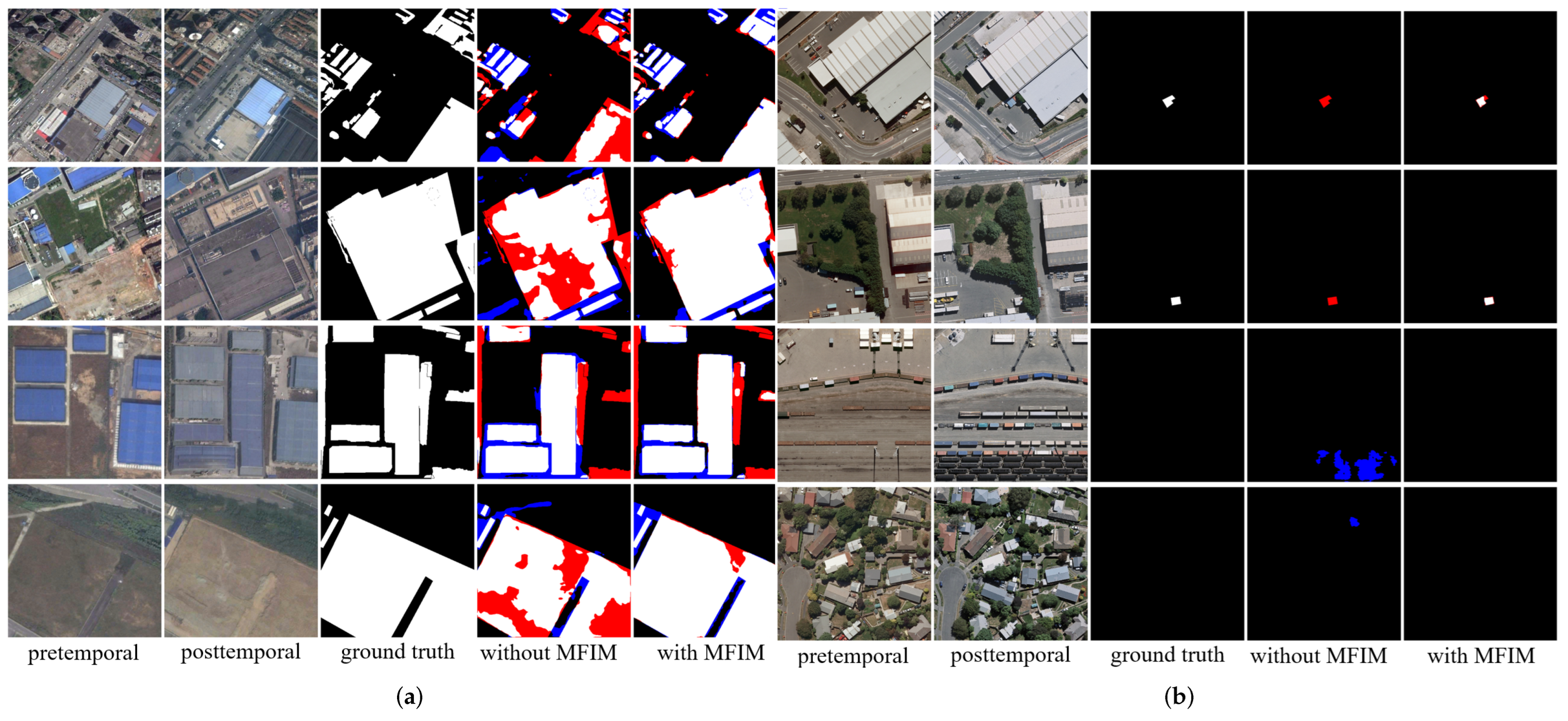
Figure 8.
Visual comparisons of the baseline without/with the MFIM. (a) Inference results on the SECOND dataset. (b) Inference results on the WHU dataset. For better visualization, we show the missing changes with red and unexpected changes with blue.
Figure 8.
Visual comparisons of the baseline without/with the MFIM. (a) Inference results on the SECOND dataset. (b) Inference results on the WHU dataset. For better visualization, we show the missing changes with red and unexpected changes with blue.

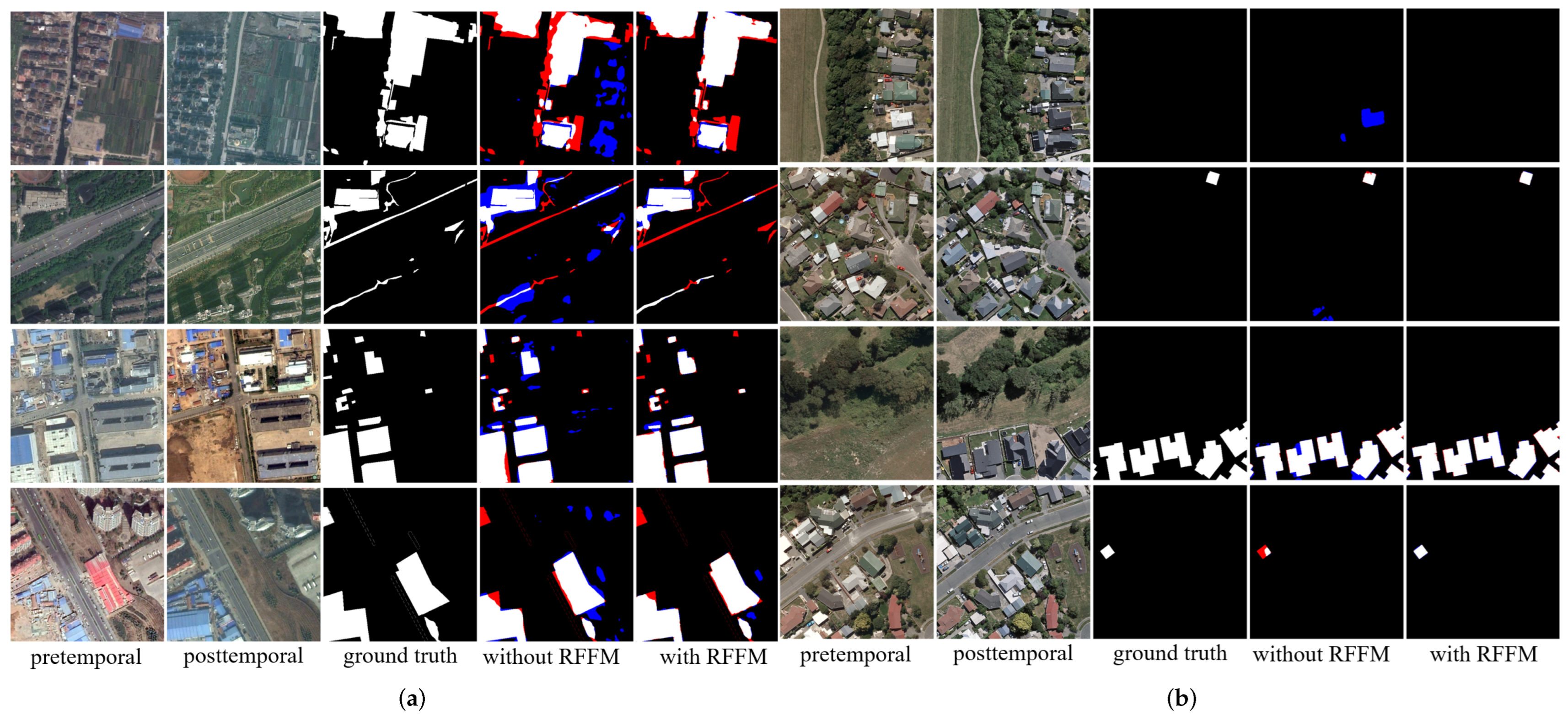
Figure 9.
Visual comparisons of baseline without/with the RFFM. (a) Inference results on the SECOND dataset. (b) Inference results on the WHU dataset. For better visualization, we show the missing changes with red and unexpected changes with blue.
Figure 9.
Visual comparisons of baseline without/with the RFFM. (a) Inference results on the SECOND dataset. (b) Inference results on the WHU dataset. For better visualization, we show the missing changes with red and unexpected changes with blue.

Figure 10.
Feature visualization with t-SNE. (a) Visualization of features without deep supervision. (b) Visualization of features with deep supervision. Dots in red and marked with 0 represent unchanged features. Dots in blue and marked with 1 represent changed features.
Figure 10.
Feature visualization with t-SNE. (a) Visualization of features without deep supervision. (b) Visualization of features with deep supervision. Dots in red and marked with 0 represent unchanged features. Dots in blue and marked with 1 represent changed features.

Figure 11.
The inferences on the SECOND dataset. (a) Pre-temporal images. (b) Post-temporal images. (c) Ground truths. (d) Inferences of FC-Sima-diff. (e) Inferences of IFN. (f) Inferences of SNUNet_CD. (g) Inferences of BiT. (h) Inferences of RFNet. We color the missing changes with red and unexpected changes with blue.

Figure 12.
Inference results on the WHU dataset. (a) Pre-temporal images. (b) Post-temporal images. (c) Ground truths. (d) Inferences of FC-Sima-diff. (e) Inferences of IFN. (f) Inferences of SNUNet_CD. (g) Inferences of BiT. (h) Inferences of RFNet. We visualize the missing changes with red and unexpected changes with blue.

Figure 13.
The way bitemporal images are shifted.

Figure 14.
Robustness comparison results on the test sets. (a) The performance with different offsets on SECOND. (b) The loss of performance with different offsets on the SECOND dataset. (c) The performance with different offsets on the WHU dataset. (d) The loss of performance with different offsets on the WHU dataset. The bias of bitemporal images ranges from 1 pixel to 5 pixels.


Table 1.
The ablation study of introducing the MFIM. The symbol ± means the performance fluctuation. The values in bold font are the best.
Table 1.
The ablation study of introducing the MFIM. The symbol ± means the performance fluctuation. The values in bold font are the best.
| SECOND | WHU | ||||||||
|---|---|---|---|---|---|---|---|---|---|
| Introduce | Precision (%) | Recall (%) | IoU (%) | F1 (%) | Precision (%) | Recall (%) | IoU (%) | F1 (%) | Params |
| MFIM | (Mb) | ||||||||
| no | 67.94 | 72.37 | 53.95 (±0.28) | 70.09 (±0.24) | 92.85 | 86.78 | 81.35 (±0.44) | 89.71 (±0.25) | 32.5 |
| yes | 72.54 | 70.37 | 55.57 (±0.31) | 71.44 (±0.27) | 95.54 | 88.41 | 84.11 (±0.27) | 91.37 (±0.11) | 39.3 |
Table 2.
The ablation study of applying the RFFM to the baseline. The symbol ± means the performance fluctuation. The values in bold font are the best.
Table 2.
The ablation study of applying the RFFM to the baseline. The symbol ± means the performance fluctuation. The values in bold font are the best.
| SECOND | WHU | ||||||||
|---|---|---|---|---|---|---|---|---|---|
| Introduce | Precision (%) | Recall (%) | IoU (%) | F1 (%) | Precision (%) | Recall (%) | IoU (%) | F1 (%) | Params |
| RFFM | (Mb) | ||||||||
| no | 67.94 | 72.37 | 53.95 (±0.28) | 70.09 (±0.24) | 92.85 | 86.78 | 81.35 (±0.44) | 89.71 (±0.25) | 32.5 |
| yes | 72.9 | 69.71 | 55.36 (±0.19) | 71.27 (±0.17) | 95.06 | 87.74 | 83.51 (±0.35) | 91.25 (±0.19) | 32.7 |
Table 3.
The ablation study of with/without deep supervise. The symbol ± means the performance fluctuation. The values in bold font are the best.
Table 3.
The ablation study of with/without deep supervise. The symbol ± means the performance fluctuation. The values in bold font are the best.
| SECOND | WHU | ||||||||
|---|---|---|---|---|---|---|---|---|---|
| Use Deep | Precision (%) | Recall (%) | IoU (%) | F1 (%) | Precision (%) | Recall (%) | IoU (%) | F1 (%) | Params |
| Supervise | (Mb) | ||||||||
| no | 72.9 | 69.71 | 55.36 (±0.19) | 71.27 (±0.17) | 95.06 | 87.74 | 83.51 (±0.35) | 91.25 (±0.19) | 32.7 |
| yes | 71.67 | 71.54 | 55.77 (±0.3) | 71.6 (±0.25) | 94.7 | 89.46 | 85.19 (±0.51) | 92 (±0.32) | 32.7 |
Table 4.
Model comparison of the SECOND dataset. The values in bold font are the best.
| Precision (%) | Recall (%) | IoU (%) | F1 (%) | Params (Mb) | |
|---|---|---|---|---|---|
| FC-EF [51] | 59.53 | 57.6 | 38.46 | 58.55 | 5.15 |
| FC-Sima-conc [51] | 61.21 | 58.33 | 42.59 | 59.74 | 5.9 |
| FC-Sima-diff [51] | 63.68 | 63.128 | 46.418 | 63.48 | 5.15 |
| CDNet [39] | 57.41 | 69.73 | 45.95 | 62.97 | 7.75 |
| UNet++_MSOF [11] | 68.74 | 58.39 | 46.14 | 63.14 | 35 |
| IFN [59] | 73.09 | 63.4 | 51.4 | 67.9 | 137 |
| SNUNet_CD [60] | 72.37 | 69.35 | 54.84 | 70.83 | 46 |
| BiT [69] | 71.12 | 72.33 | 55.91 | 71.72 | 45.8 |
| RFNet (ours) | 74.15 | 71.46 | 57.21 | 72.78 | 39.4 |
Table 5.
Model comparison of the WHU dataset. The values in bold font are the best.
| Precision (%) | Recall (%) | IoU (%) | F1 (%) | Params (Mb) | |
|---|---|---|---|---|---|
| FC-EF [51] | 78.58 | 78.13 | 64.41 | 78.35 | 5.15 |
| FC-Sima-conc [51] | 76.19 | 73.35 | 59.68 | 74.75 | 5.9 |
| FC-Sima-diff [51] | 84.03 | 83.24 | 70.63 | 83.63 | 5.15 |
| CDNet [39] | 82.86 | 78.3 | 67.39 | 80.52 | 7.75 |
| UNet++_MSOF [11] | 86.7 | 80.25 | 71.45 | 83.35 | 35 |
| IFN [59] | 94.81 | 86.5 | 82.59 | 90.47 | 137 |
| SNUNet_CD [60] | 90.07 | 88.23 | 80.4 | 89.14 | 46 |
| BiT [69] | 85.31 | 91.06 | 78.72 | 88.09 | 45.8 |
| RFNet (ours) | 95.72 | 89.46 | 86.02 | 92.49 | 39.4 |
Publisher’s Note: MDPI stays neutral with regard to jurisdictional claims in published maps and institutional affiliations. |
© 2022 by the authors. Licensee MDPI, Basel, Switzerland. This article is an open access article distributed under the terms and conditions of the Creative Commons Attribution (CC BY) license (https://creativecommons.org/licenses/by/4.0/).
Share and Cite
MDPI and ACS Style
Chen, P.; Li, C.; Zhang, B.; Chen, Z.; Yang, X.; Lu, K.; Zhuang, L. A Region-Based Feature Fusion Network for VHR Image Change Detection. Remote Sens. 2022, 14, 5577. https://0-doi-org.brum.beds.ac.uk/10.3390/rs14215577
AMA Style
Chen P, Li C, Zhang B, Chen Z, Yang X, Lu K, Zhuang L. A Region-Based Feature Fusion Network for VHR Image Change Detection. Remote Sensing. 2022; 14(21):5577. https://0-doi-org.brum.beds.ac.uk/10.3390/rs14215577
Chicago/Turabian StyleChen, Pan, Cong Li, Bing Zhang, Zhengchao Chen, Xuan Yang, Kaixuan Lu, and Lina Zhuang. 2022. "A Region-Based Feature Fusion Network for VHR Image Change Detection" Remote Sensing 14, no. 21: 5577. https://0-doi-org.brum.beds.ac.uk/10.3390/rs14215577
Note that from the first issue of 2016, this journal uses article numbers instead of page numbers. See further details here.