Monitoring Asbestos Mine Remediation Using Airborne Hyperspectral Imaging System: A Case Study of Jefferson Lake Mine, US

Abstract

This study investigated an asbestos mine restoration project using Airborne Visible/Infrared Imaging Spectrometer (AVIRIS) hyperspectral data. The distribution of an abandoned asbestos mine (AAM) and treatment area were analyzed before and after the remediation based on the spectral indices for detecting naturally occurring asbestos (NOA) indicators and encapsulation. The spectral indices were developed for NOA, host rock, and encapsulation by logistic regression models using spectral bands extracted from the random forest algorithm. The detection models mostly used VNIR spectra rather than SWIR and were statistically significant. The overall accuracy of the detection models was approximately 84%. Notably, the detection accuracy of non-treated and treated areas was increased to about 96%, excluding the host rock index. The NOA index detected asbestos in the mine area as well as those in outcrops outside of the mine. It has been confirmed that the NOA index can be efficiently applied to all cases of asbestos occurrence. The remote sensing data revealed that the mine area was increased by ~5% by the remediation, and the treatment activity reduced asbestos exposure by ~32%. Moreover, the integrative visualization between the detection results and 3D high-resolution images provided an intuitive and realistic understanding of the reclamation project.

1. Introduction

Naturally occurring asbestos (NOA) minerals can be classified into serpentine (chrysotile) and amphibole (actinolite, amosite, anthophyllite, crocidolite, and tremolite) groups. They are known to cause serious health damage to human body systems, as forms of lung diseases, such as mesothelioma and pneumoconiosis [1,2,3,4]. Due to their harmful impact, the production/distribution of asbestos minerals is banned in many countries under strict environmental regulations [5].

The Environmental Protection Agency (EPA) in the United States has been extensively managing asbestos-related sites with significant attention to abandoned asbestos mines (AAM). Systematic cleanup activities have been regulated as a national priorities list (NPL). Due to the significance of NOA in both environment and ecology, a survey of NOA in both natural and mine environments is a critical procedure to prevent its dispersion. EPA has introduced mine cleanup strategies according to the type of mining processes, such as open pit, dredging, and underground to minimize exposure [6]. Major mine remediation includes chemical, physical, and thermal treatment to limit the mobility of contaminants [6]. Therefore, the assessment of the remediation work in terms of NOA exposure before and after the remediation is critical.

Traditionally, field-based conventional surveys have been the main protocol for NOA surveys, which include sampling, pre-processing, microscopic observation, and mineralogical analysis. Thus, it requires considerable time, cost, and labor, and is hard to understand the spatial distribution of NOA with a small amount of point-based sampling [7]. A hyperspectral imaging system (HIS) in visible-near infrared (VNIR: 400 to 1400 nm) to short wave infrared (SWIR: 1400 to 2500 nm) regions could be an alternative solution for asbestos mineral exploration, offering prompt detection of complete spatial coverage. HIS can be mounted on multi-latitude platforms, including close-range, ground, UAV, airborne, and spaceborne remote sensing. Notably, the HIS approach could detect spectral characteristics of NOAs promptly at a low cost [7,8,9,10].

Previous studies on hyperspectral remote sensing for asbestos mapping have mainly focused on investigations of building materials (e.g., asbestos-cement (AC)) in a residential area. Multispectral infrared visible imaging spectrometer (MIVIS) data have been mainly used for the detection of AC based on classification algorithms, including spectral angle mapper (SAM) and spectral feature fitting (SFF) [5,11,12,13]. They mapped AC roofs, a mixture of asbestos-containing (e.g., chrysotile and crocidolite) material in cement, with 80~90% accuracy based on ground samples. Additionally, Krówczyńska (2020) and Raczko (2022) tried to identify AC-roofing using convolutional neural networks (CNNs) based on high-resolution aerial photos [14,15]. They proved a detection level at an accuracy ranging from 87 to 93%.

In 2004, a joint survey between the United States Geological Survey (USGS) and the California Geological Survey (CGS) used the Airborne Visible/Infrared Imaging Spectrometer (AVIRIS) for NOA mapping and focused on imaging NOA-bearing rocks within a vegetated area based on the mineral spectral characteristics [2]. They used the Tetracorder system, a hyperspectral classification program developed by USGS, to identify the potential of NOA occurrences, such as serpentine- and tremolite–actinolite-bearing rocks [2,16,17,18].

Although previous studies have investigated remote sensing for the asbestos survey, there is no study on the remediation assessment of AAM. The previous studies only focused on AC roof monitoring. However, the AC studies could not be applicable for AAM detection due to differences in spectral characteristics. Furthermore, the limited number of case studies on NOA could not be used for AAM monitoring as they did not consider the remediation area. Indeed, the critical aspect of AAM remediation is to decide if the treatment could prevent NOA dispersion efficiently. The remediation commonly uses an encapsulated-solidification method to cover the AAM exposure, and, thus, it is important to figure out the distribution of AAM itself rather than the identification of individual NOA rocks and minerals. The AAM detection requires an understanding of geological characteristics composing the mine area. In other words, it would be critical to derive an indicator of NOA materials, including asbestos minerals and host rocks. Then, an assessment of the persistence of the NOA traces after the treatment must be conducted.

This study investigated an AAM restoration project on the Jefferson Lake mine, CA, US, using airborne hyperspectral remote sensing data. The distribution of AAM and solidification area were analyzed before and after the remediation process. The spectral indices for the detection of the NOA indicator (NOAI hereafter) and the encapsulation (CAP hereafter) were developed and validated for the AAM remediation monitoring. This is the first study on the assessment of AAM remediation projects and expects to contribute as a reference for future remediation projects and maintenance.

2. Materials and Methods

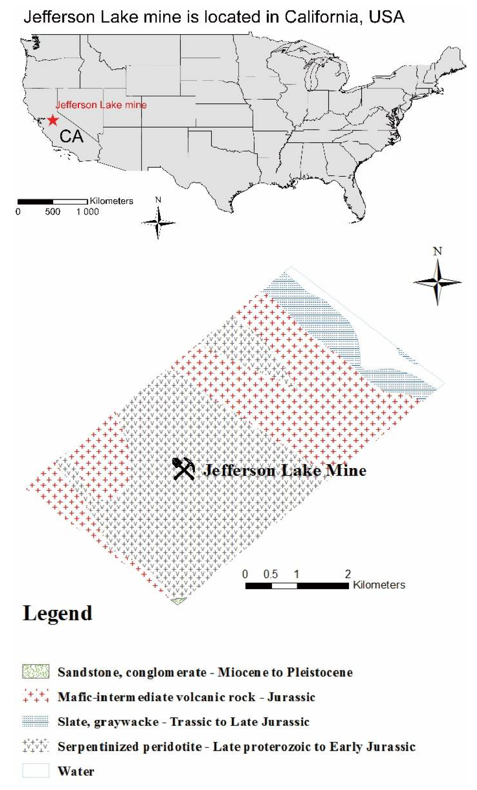
2.1. Study Area

This study investigated an AAM restoration project on Jefferson Lake mine (owned by Jefferson Lake Asbestos Corporation) to assess mine cleanup activities. The Jefferson Lake mine, located in Calaveras county, had been one of the largest asbestos producers, operated from 1962 to 1987 [19] (Figure 1).

2.1.1. Geology

The geology of the study area is composed of four main rock units (Figure 1). Late Proterozoic to Early Jurassic ultramafic rock, as the host rock of the asbestos mine, is located at the center of the study area. The host rock is surrounded by Triassic to Late Jurassic slate–graywacke. The rock units were intruded by Jurassic intrusive rock. The later Miocene to Pleistocene sandstone–conglomerate covers the bedrocks as unconformity (Figure 1).

The host rock of the Jefferson Lake mine is a metasomatized ultramafic rock [20]. The host rock is mainly composed of iron–magnesium silicate minerals, such as olivine and pyroxene, and partially altered amphibolite, dunite, peridotite, and serpentinite [19]. The asbestos minerals in the mine are formed by the serpentinization of the ultramafic rocks (Figure 1) [19,21]. This process alters the original iron–magnesium minerals to water-bearing magnesium silicate minerals, such as antigorite, chrysotile, and lizardite, the serpentine asbestos mineral group [19,22].

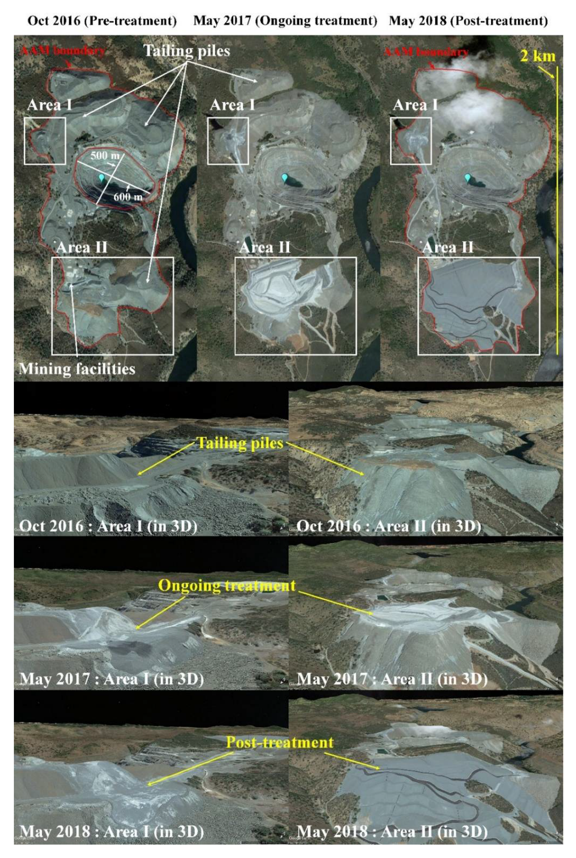
2.1.2. Mine Cleanup Activity of the Study Area

After a ban on asbestos materials, the NOA mines in CA have been assessed by environmental quality investigations [19]. The open pit of Jefferson Lake mine (also called Copperopolis chrysotile mine and/or Calaveras mine) was used as an asbestos disposal site for mine reclamation [19,23]. As the high-resolution satellite images in Figure 2 show, the piles of tailings were distributed around the open pit location, and Areas I and II are the main reclamation sites. The reclamation is visible in the 2017 image, while the 2016 image shows the pre-reclamation condition. The major reclamation took place with paved preparation and finished in 2018 (Figure 2).

The high-resolution images show that treatment sites 1 and 2 were completely changed and encapsulated for both areas (Figure 2). Notably, Area II is confirmed as the main tailing pile site with mining facilities (Figure 2). The EPA’s remediation and cleanup protocol for AAM officially follows a solidification method for minimum surface exposure with encapsulation to prevent dispersion of asbestiform [6]. In Figure 2, the AAM remediation activities using encapsulated solidification are finished for the study site in 2018.

The overall AAM site measures 2 km in diameter with a major mining open pit located at the center (Figure 2). The area of AAM was about 1.73 km² and that of the open pit was 0.23 km² in 2016, and the AAM area had been extended to 1.81 km², a 5% increase, including the treatment area due to reclamation activities in 2018 (Figure 2).

2.2. AVIRIS Data

AVIRIS is an airborne hyperspectral sensor which has operated since the late 1980s. This study used a radiometrically corrected AVIRIS Level 2 product to map asbestos exposure and encapsulation operation. The atmospheric correction was conducted by the Atmosphere Removal Algorithm (ATREM) developed by Gao et al. (1993) [24,25]. It retrieves a scaled surface reflectance by modeling the absorption due to atmospheric effects [26]. Furthermore, an empirical line method is used to correct the surface reflectance using reference targets measured in the field [26]. AVIRIS data used in this study are summarized in

Table 1. AVIRIS data description used in this study.

Product ID (Acquisition Date)	Spectral Resolution	Number of Bands	Wavelength (nm)	GSD (m)	Scanning Type	Nominal Altitude (km)	Swath (km)
f140602t01p00r07 (2 June 2014)	~10 nm	224	366 to 2495	14.5	Whisk broom	20	11
f180621t01p00r05 (21 June 2018)				14.4

.

This study selected AVIRIS data acquired in 2014 and 2018 for comparative analysis before and after the treatment. Ground sample distance (GSD) was unified at 14.4 m by image resampling, and geometric calibration, UTM projection, and clipping for the open pit area were applied to the images to make a consistent-spatial comparison.

2.3. Multi-Range Spectral Feature Fitting (MRSFF)

In the study area, the asbestos occurrences originated from the serpentinization of dunite–peridotite (mainly composed of olivine and pyroxene). Serpentinization could form lizardite, chrysotile, and antigorite as secondary minerals [22,27]. To analyze possible mineral candidates and spectral characteristics representing the AAM area, reference spectra were collected from USGS spectral library 7. The collected reference spectra were grouped to develop a host rock indicator (HRI hereafter) and an NOA indicator (NOAI hereafter), where HRI is comprised of olivine (forsterite–fayalite series) and pyroxene (augite) and NOAI represents lizardite, chrysotile, antigorite, and serpentine [28]. The reference numbers of the spectra are summarized in Appendix A. The reference spectra were averaged and resampled to the AVIRIS bandpass and transformed into continuum-removed (CR) reflectance to enhance absorption features. The bad bands from 1260 to 1560 nm and 1740 to 1956 nm were excluded for spectral analysis and model development.

The HRI and NOAI mineral spectra were used for end-member extraction from AVRIS data by multi-range spectral feature fitting (MRSFF). The SFF is commonly used to detect image pixels closest to reference spectra based on spectral similarity (a least-square fitting model). MRSFF is an enhanced SFF method appropriate for the detection of a subtle spectral feature with better accuracy [29]. It uses the weighted least-squares method for the multi-wavelength ranges where weighting is given based on a minimum error (RMSE) [29].

The NOAI spectrum collected from the USGS spectral library showed distinct strong absorptions at about 2100, 2300, and 2400 nm (Figure 3). The absorption features in SWIR regions are manifested by Al-, Fe-, and Mg-OH chemical bonds associated with alteration minerals (Figure 3) [30,31,32,33]. On the other hand, HRI relatively showed a flattened spectral pattern in SWIR, but a broad absorption by ferric/ferrous components (Fe²⁺ and Fe³⁺) in the VNIR is observed (Figure 3). The distinctive differences between NOAI and HRI explain that the asbestos-forming materials can be spectrally differentiated in a mixture with host rock compositions in the AAM area. Based on these spectral differences, the weighted-multi ranges for MRSFF were considered to extract end-member pixels. In Figure 3, the wavelength ranges marked in blue and orange color blocks indicate the major spectral features’ regions for differentiating NOAI and HRI, as well as the multi ranges for MRSFF. The multi ranges are 753 to 879, 908 to 1263, and 2247 to 2436 nm for HRI and 2067 to 2197 and 2237 to 2426 nm for NOAI (Figure 3). They overlap each other at ~2300 nm but do not overlap in the VNIR ranges. This infers that both VNIR and SWIR regions should be included in separating NOAI and HRI.

MRSFF results produce RMSE and scale images. The scale factor indicates an abundance of target spectral features where greater scale values represent stronger absorptions. In other words, the low RMSE and high scale factors indicate the closest matching of the target material’s spectral signature. We extracted end-member pixels for HRI and NOAI by selecting those at the top 10% scale factor values and lower 10% RMSE values. Moreover, the remediation areas defined as CAP class were extracted from visual inspection of the high-resolution images. Then, the surface features, except for HRI, NOAI, and CAP, such as bare soil, vegetation, road, and stream, were delineated as the other class (Others hereafter). As a result, a total of 403, 218, 676, and 8680 pixels were extracted from 2018 AVRIS data representing the NOAI, HRI, CAP, and Others classes, respectively.

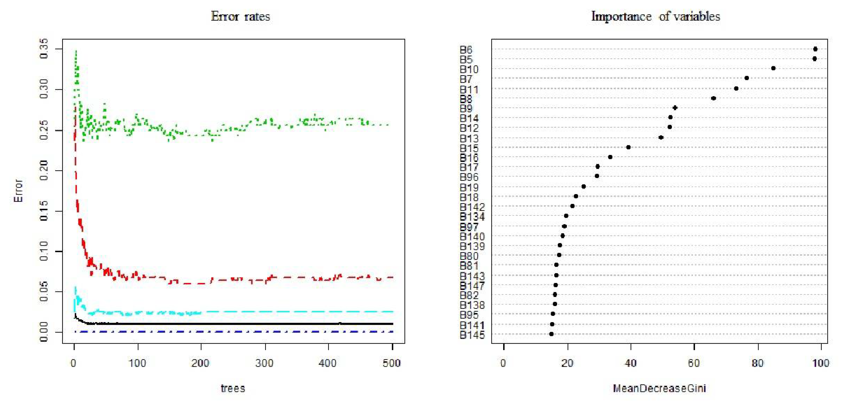
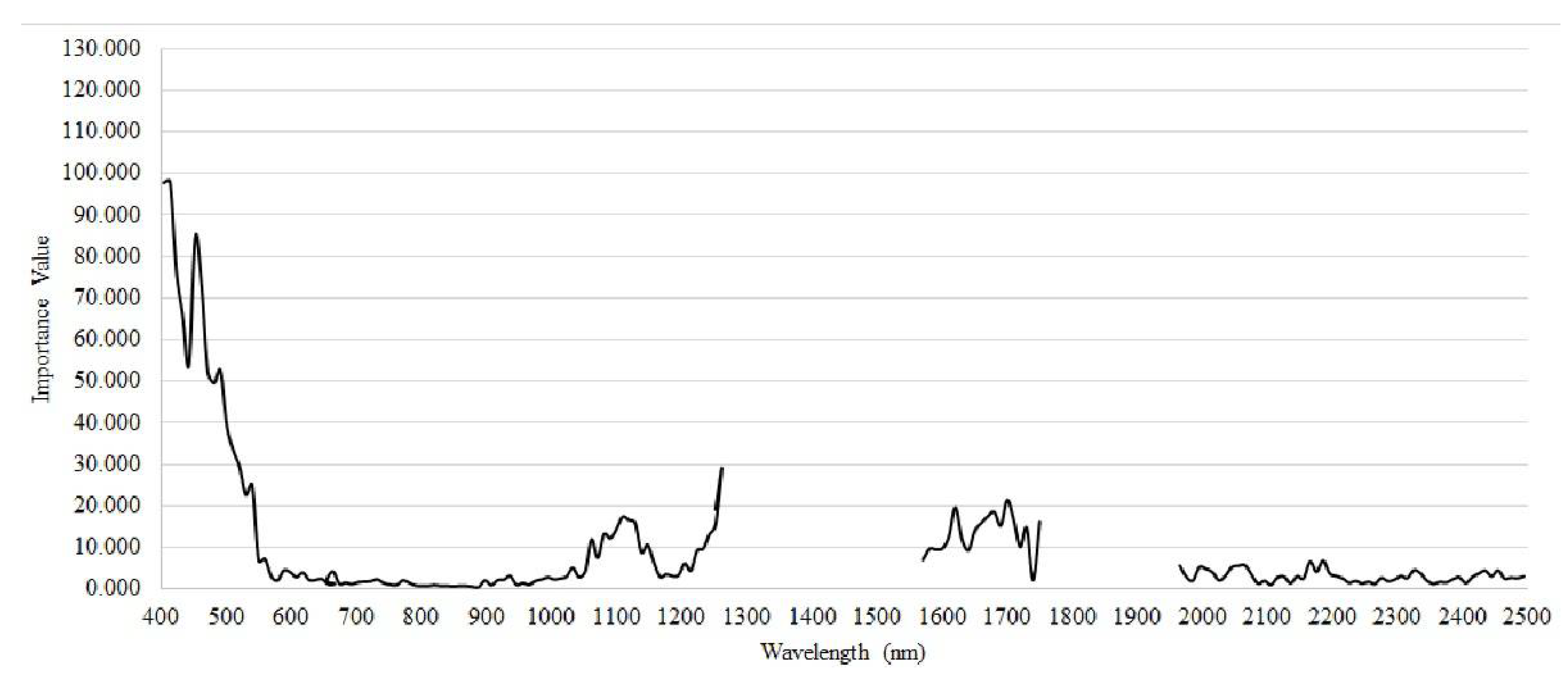
2.4. Band Selection and Model Development

To develop the spectral indices for NOAI, HRI, and CAP, we selected responsive spectral bands using a random forest (RF hereafter) algorithm. The RF classification algorithm is an ensemble of classification trees where a majority vote from each tree assigns the class to each case [9,34,35]. It is based on bagging and bootstrapping for generating trees by repeating the randomized formation of variable sets [9,36]. Notably, the RF yields important variables for the classification indicated by the Gini and out-of-bag (OOB) error value. The lower errors indicate the more important variable for classifying with the best split [35,37]. Based on the RF algorithm report, we selected the top 30 spectral bands with the lowest OOB errors for developing spectral indices with the BLR model [9].

Based on the spectral bands sensitive to class differentiation, the spectral indices were derived from BLR which calculates the probability of an event based on a binary operator [38]. The probability is defined as:

$${\mathrm{Prob}}_{\mathrm{class}}=\frac{{\mathrm{e}}^{(\mathrm{C}+{\mathsf{\beta }}_{1\times 1}+{\mathsf{\beta }}_2{x}_2+{\mathsf{\beta }}_3{x}_3+\cdots +{\mathsf{\beta }}_{\mathrm{n}}{x}_{\mathrm{n}})}}{{1+\mathrm{e}}^{(\mathrm{C}+{\mathsf{\beta }}_1{x}_1+{\mathsf{\beta }}_2{x}_2+{\mathsf{\beta }}_3{x}_3+\cdots +{\mathsf{\beta }}_{\mathrm{n}}{x}_{\mathrm{n}})}}$$

(1)

where Prob_class is the probability of the target class occurrence, C indicates the constant value of the equation, β_n is the coefficient of the predictor variables, and x_n is the wavelength band selected from the regression. The probability is exponentially calculated by ranging from 1 to 0. In this study, the binary logic for class occurrence is determined by a probability higher than 0.5 [9].

The suitability of BLR models was assessed by the Hosmer–Lemeshow test, Wald statistics, and R² values of Cox–Snell (CS) and Nagelkerke (N). The Hosmer–Lemeshow test is a goodness of fit (prediction) test based on an evaluation of the p-value. This test divides the samples into deciles and assesses the statistical significance of the model by the probability of matching between observed and predicted values. The R² of Cox and Snell (2018) and Nagelkerke (1991) can be expressed as (2) and (3), respectively [39,40,41]:

$$R_{\mathrm{CS}}^2=1-{\left(\frac{{\mathrm{L}}_1}{{\mathrm{L}}_0}\right)}^{\raisebox{1ex}{$2$}\!\left/ \!\raisebox{-1ex}{$n$}\right.}$$

(2)

$$R_N^2 =\frac{R_{\mathrm{CS}}^2}{{1-{\mathrm{L}}_0}^{\raisebox{1ex}{$2$}\!\left/ \!\raisebox{-1ex}{$n$}\right.}}$$

(3)

where n is the sample size, L₀ and L₁ represent the likelihoods of the fitted and the null model (intercept only), and CS and N indicate Cox–Snell and Nagelkerke. The ratio calculation closing to 1 means a high explanatory power of the model. We selected the best logistic equation with the highest R² and prediction accuracy [9,42].

The logistic regression models were developed based on 70% of pixels for each class (282, 152, and 473 pixels for NOAI, HRI, and CAP). The remaining 30% of the pixels (121, 66, and 203 pixels for NOAI, HRI, and CAP) were used for validation. Separately from the validation-set, a test-set for cross-validation of the models was constructed by extracting 50% of the class pixels (121, 66, and 338 pixels for NOAI, HRI, and CAP). The accuracy of the models was assessed by the confusion matrix of both the validation and test dataset. The image processing and model development were conducted by R 3.5.3, ArcGIS Pro, ENVI 5.6.2, IDL 8.5, and SPSS 26.

3. Results and Discussion

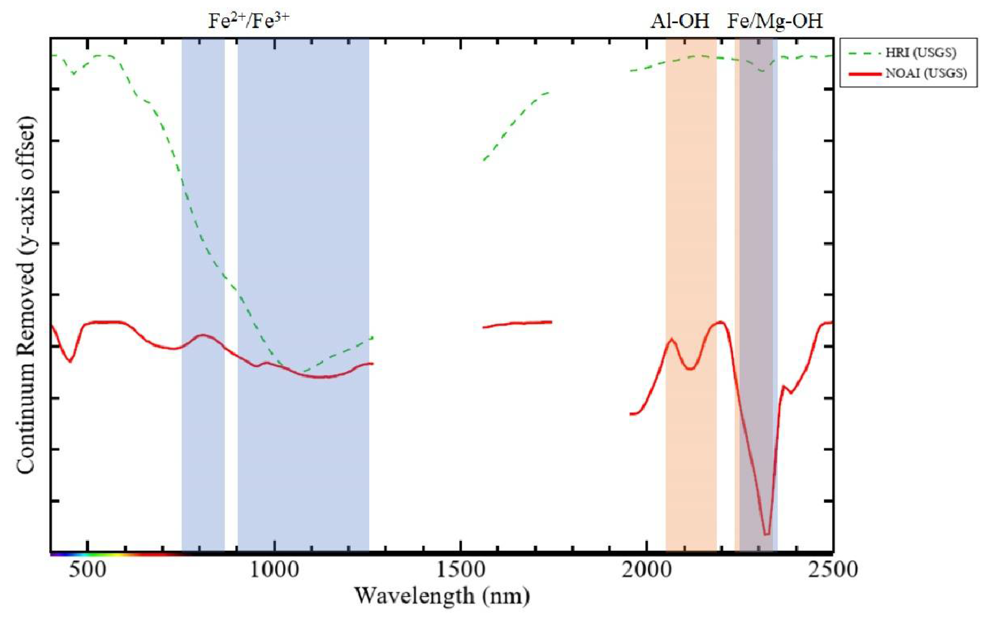
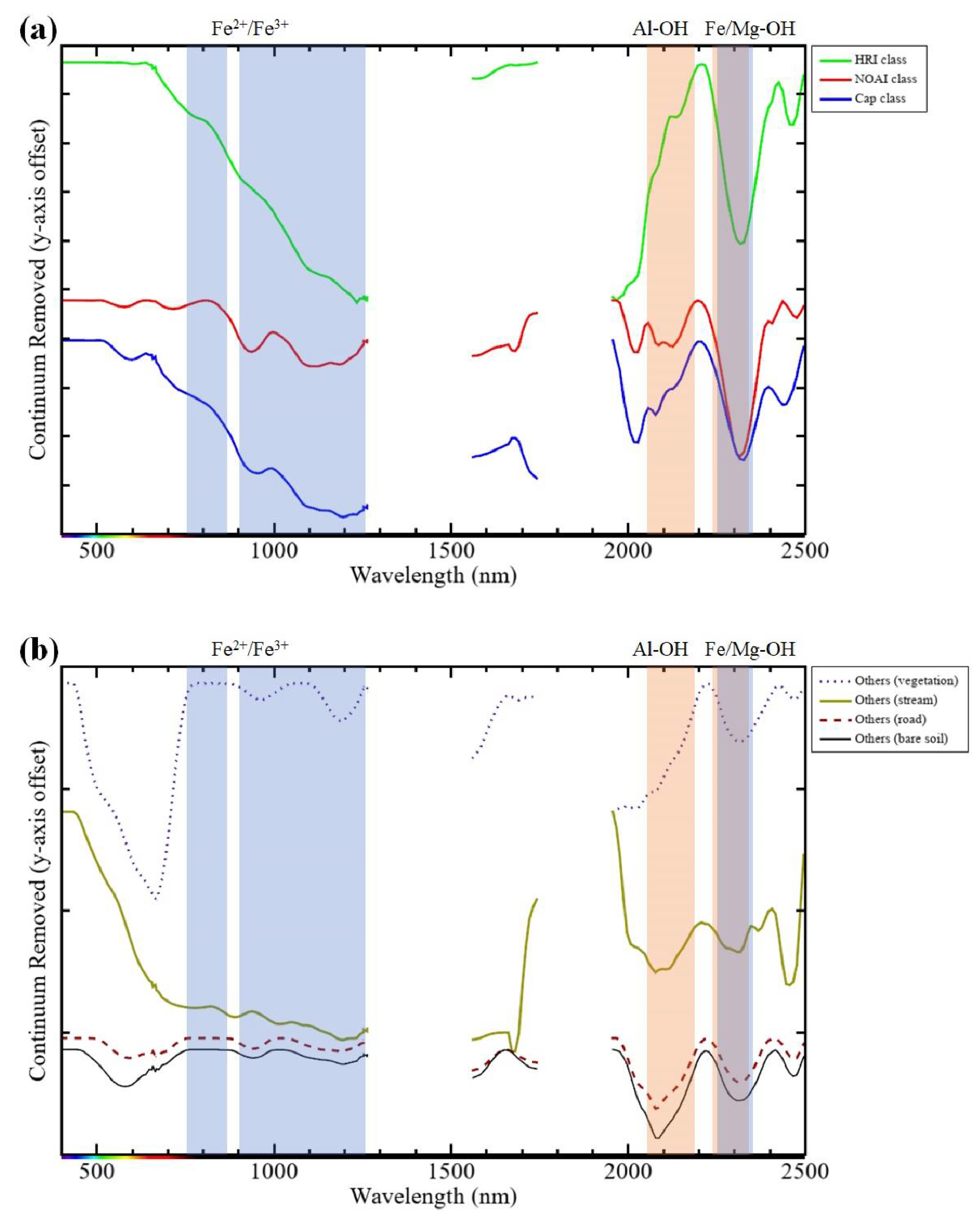
3.1. Spectral Characteristics of AAM and Remediation Area

The extracted end-member image pixels for HRI, NOAI, and CAP classes are compared in Figure 4a. In comparison with HRI and NOAI in Figure 3, the absorptions in ~450 to 470 nm have been not detected and small absorptions are shown as higher band depth in the absorption. The difference might be originated from the effects of the data precision and various mineral assemblages in the natural environment.

As defined previously, the NOAI and HRI classes comprise AAM. NOAI and HRI share similar absorption locations in the SWIR region. In the VNIR region, although none of them have strong absorption features, the curves have different shapes. Similar spectral characteristics in SWIR can be explained by occurrence patterns in real cases, where NOA and host rock compositions occur as a mixture. On the other hand, the distinctive VNIR spectral characteristics of HRI indicate a more abundant host rock composition than the NOAI effect. This means that the spectrum of HRI indicates predominant host rock composition but a co-existed small amount of NOA containing Al-, Fe-, and Mg-OH can spectrally affect the SWIR region because these chemical bonds are infrared-active. Indeed, Jeong et al. (2016) have discussed that the spectral features of multiple minerals can coexist in a single spectrum, and the detection of minerals with a weaker spectral characteristic than infrared-active minerals (e.g., alteration and asbestos minerals) should integrate VNIR characteristics as supplementary information [30]. It implies that both VNIR and SWIR are useful to separate NOAI and HRI. The CAP class also has a strong absorption at ~2300 nm and shows a similar absorption pattern to the NOAI in the SWIR region (Figure 4a). Again, in the VNIR region, the CAP class showed a different spectral trend in ~600 to 1200 and ~1600 to 1700 nm (Figure 4a). These spectral differences between the NOAI and CAP classes would enhance remediation monitoring. Moreover, compared to the NOAI, HRI, and CAP classes, although the Others class, including vegetation, stream, road, and bare soil, has common absorption positions and shapes at ~1200 and ~2300 nm, they showed a different pattern over whole spectral regions (Figure 4b). This gives a prospect that the Others class can be spectrally isolated from NOAI, HRI, and CAP classes.

3.2. Binary Logistic Regression Models

3.2.1. Classification Models

The RF algorithm reported variables’ Gini values (Figure 5). The top 30 bands with the highest Gini value reduction were selected, which are mainly distributed over the VNIR region, except ~1600 to 1700 nm from the SWIR region (Figure 6). This result confirms the conclusion from the visual spectral analysis in Section 3.1 that the VNIR bands are useful for AAM remediation monitoring. In general, VNIR bands provide better spectral and spatial resolutions because of their high N/S ratio and strong energy flux in a natural environment. This finding will facilitate building sensors for AAM reclamation monitoring at multiple platforms, such as UAV, aerial, and space-borne. It is especially important for projects using satellite systems because of the far distance and atmospheric degradation.

The parameter-ntrees are selected at 100 because the error rates became non-incremental when ntrees > 100 (Figure 5). The error rates are 0.07, 0.26, 0.03, and 0.00 for the NOAI, HRI, CAP, and Others, respectively (Figure 5). Overall, the HRI had the lowest accuracy, while other classes are more separable.

The step-wise selection of the logistic regression variables for each of the classes, NOAI, HRI, and CAP, determined the best models for each, which used 9, 7, and 4 spectral variables picked from the 30 candidates with statistical suitability (p-value < 0.05) (

Table 2. NOAI logistic model parameters derived from BLR and Wald test.

Band NO.	Wavelength (nm)	β	S.E.	Wald	Df	p-Value
B5	405	373.559	58.167	41.244	1	0.000
B10	453	−716.856	187.971	14.544	1	0.000
B12	473	−1230.725	235.065	27.412	1	0.000
B16	511	1691.958	171.184	97.691	1	0.000
B19	541	−184.665	61.111	9.131	1	0.003
B134	1622	561.510	152.744	13.514	1	0.000
B138	1662	−668.925	150.974	19.631	1	0.000
B139	1671	−572.095	170.551	11.252	1	0.001
B143	1711	665.147	99.788	44.430	1	0.000
Constant	-	4.547	1.036	19.247	1	0.000

β = logistic coefficient; S.E. = standard error of estimate; Wald = Wald chi-square values; Df = degree of freedom; p-value = statistical probability level (<0.05).

,

Table 3. HRI logistic model parameters derived from BLR and Wald test.

Band NO.	Wavelength (nm)	β	S.E.	Wald	Df	p-Value
B5	405	−134.266	29.586	20.595	1	0.000
B19	541	100.338	23.719	17.896	1	0.000
B81	1120	316.375	60.251	27.573	1	0.000
B96	1262	−525.518	63.409	68.686	1	0.000
B138	1661	−647.859	76.692	71.362	1	0.000
B145	1731	437.208	130.221	11.272	1	0.001
B147	1751	409.582	138.745	8.715	1	0.003
Constant	-	−3.432	0.571	36.156	1	0.000

β = logistic coefficient; S.E. = standard error of estimate; Wald = Wald chi-square values; Df = degree of freedom; p-value = statistical probability level (<0.05).

and

Table 4. CAP logistic model parameters derived from BLR and Wald test.

Band NO.	Wavelength (nm)	β	S.E.	Wald	Df	p-Value
B6	414	−899.369	204.914	19.263	1	0.000
B8	434	1284.501	267.707	23.022	1	0.000
B13	482	855.106	200.755	18.143	1	0.000
B19	541	−1088.831	132.396	67.635	1	0.000
Constant	-	−17.949	1.468	149.396	1	0.000

β = logistic coefficient; S.E. = standard error of estimate; Wald = Wald chi-square values; Df = degree of freedom; p-value = statistical probability level (<0.05).

). Both NOAI and HRI models employed both VNIR and SWIR variables, whereas the CAP model only used VNIR variables (Table 2, Table 3 and Table 4).

Table 5. The model summary and evaluation result.

Class	Pseudo-R2		Hosmer and Lemeshow Test
	Cox and Snell (CS)	Nagelkerke (N)	χ2	Df	p-Value
NOAI	0.235	0.819	1.709	8	0.989
HRI	0.124	0.656	3.690	8	0.884
CAP	0.370	0.947	0.742	8	0.999

shows the goodness of fit of the models. The NOAI and CAP showed statistical significance in the power of explanatory (R²) and probability levels (p-value) (the higher both values are indicates well statistical determination [9,43]), but the HRI model has relatively lower R² in CS.

The overall accuracy of the three detection models was 84.10% for validation data and 84.41% for calibration data with a kappa coefficient of 0.74 for both cases (

Table 6. Confusion matrix of the validation and test dataset for NOAI, HRI, and CAP classification models applied to 2018 AVIRIS.

Dataset	Class	Producer’s Accuracy (%)	User’s Accuracy (%)	Commission Error (%)	Omission Error (%)
Validation-set	NOAI	89.26	78.26	21.74	10.74
	HRI	31.82	84.00	16.00	68.18
	CAP	98.03	94.76	5.24	1.97
Overall accuracy: 84.10% (328/390 pixels) Kappa coefficient: 0.74
Test-set	NOAI	85.57	80.00	20.00	14.43
	HRI	43.12	78.33	21.67	56.88
	CAP	97.04	96.19	3.81	2.96
Overall accuracy: 84.41% (547/648 pixels) Kappa coefficient: 0.74

). However, the HRI model showed a low producer’s accuracy resulting from the misclassification of HRI class to NOAI class (Table 6). Although the producer’s accuracy may be unacceptable, the combination of NOAI and HRI would be still useful for the detection of AAM. Indeed, most AAMs consist of NOAs and host rocks in terms of geological distribution. The logistic regression results are similar to the RF results by showing that the HRI class could have much lower accuracy than the other two classes. This result might be caused by differences in spectral characteristics for NOAI and HRI minerals in the VNIR region and indicates that it may provide statistical error to detect host rock composition in the mixture with NOA. If the HRI is excluded, the detection of NOAI and CAP showed an accuracy higher than 94% (

Table 7. Confusion matrix of the validation and test dataset for NOAI and CAP classification models applied to 2018 AVIRIS.

Dataset	Class	Producer’s Accuracy (%)	User’s Accuracy (%)	Commission Error (%)	Omission Error (%)
Validation-set	NOAI	91.74	96.52	3.48	8.26
	CAP	98.03	100.00	0.00	1.97
Overall accuracy: 95.68% (310/324) Kappa coefficient: 0.91
Test-set	NOAI	90.55	95.79	4.21	9.45
	CAP	97.04	100.00	0.00	2.96
Overall accuracy: 94.62% (510/539 pixels) Kappa coefficient: 0.89

). Because the main objective of this study is to monitor the AAM area and remediated area, the model accuracies are commendable (Table 7).

Using Appendix B, the Others class BLR model and accuracy are presented in

Table A1. Others class logistic model parameters derived from BLR and Wald test.

Band NO.	Wavelength (nm)	β	S.E.	Wald	Df	p-Value
B5	405	−314.451	139.724	5.065	1	0.024
B17	521	−257.223	61.485	17.502	1	0.000
B96	1263	112.147	27.289	16.889	1	0.000
Constant	-	19.694	4.823	16.671	1	0.000

Model evaluation result: Pseudo-R² = 0.536 and 0.996 for CS and N; p-value of Hosmer and Lemeshow test = 1.000.

and

Table A2. Confusion matrix of the validation and test dataset for the Others class classification model applied to 2018 AVIRIS.

Dataset	Class	Producer’s Accuracy (%)	User’s Accuracy (%)	Commission Error (%)	Omission Error (%)
Validation-set	Other	100.00	100.00	0.00	0.00
Overall accuracy: 100.00% (2604/2604 pixels)
Test-set	Other	99.98	100.00	0.00	0.02
Overall accuracy: 99.98% (4339/4340 pixels)

, respectively. The accuracy showed ~99% for the Others class. This corresponded with the error rate in RF and spectral independence in the VNIR-SWIR area. It implies that the other materials in the study area would not affect the monitoring of AAM cleanup activity.

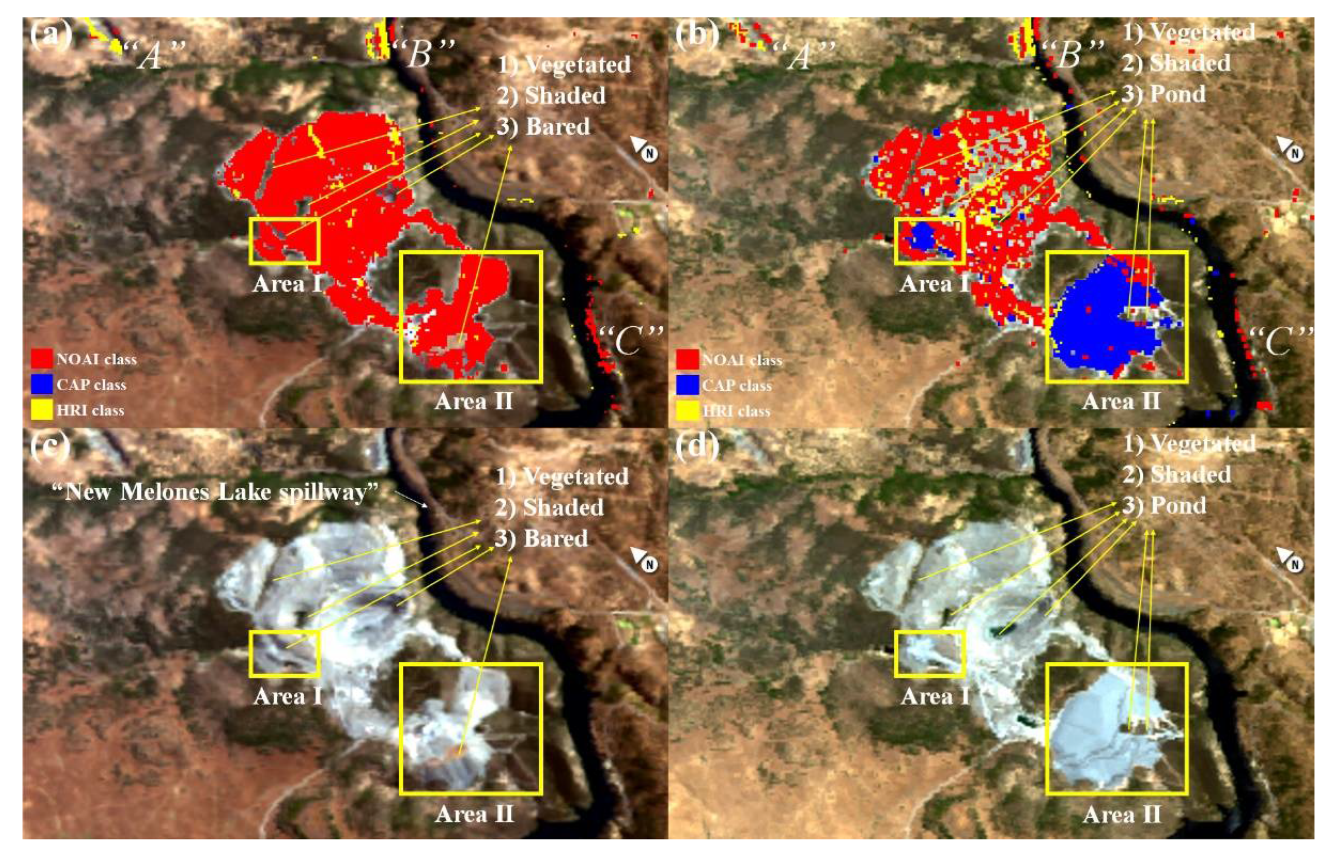
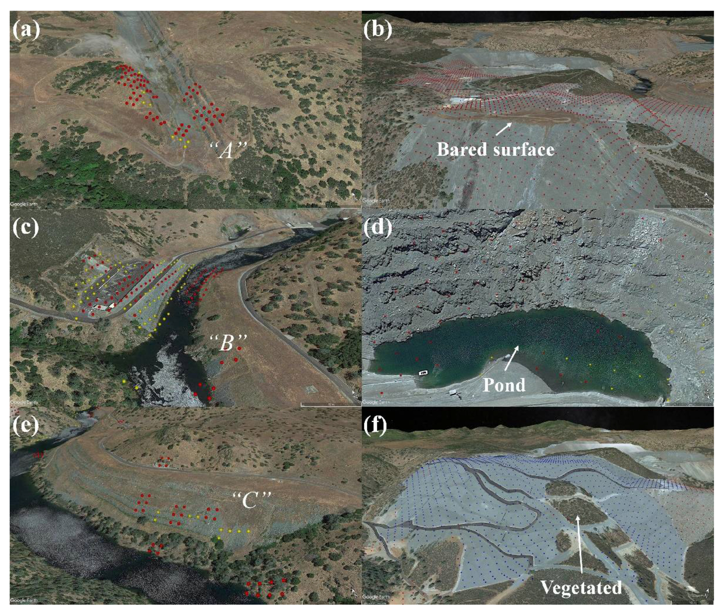
3.2.2. Spatial Assessments of the Remediation

We applied the logistic regression models from the last section to the 2014 and 2018 AVRIS data for detecting the AAM area (Figure 7). NOAI and HRI areas were mainly detected within the AAM boundary for both 2014 and 2018 data (Figure 7a,b). Notably, three areas (A, B, and C) outside of the AAM boundary were detected as NOAI and HRI class distribution (Figure 7a,b). Areas B and C are associated with spillways. Indeed, the New Melones Lake spillway was reported as one of the NOA occurrence areas in Calaveras county located in the Sierra Nevada metamorphic belt [19,44]. It confirms that the NOAI model can detect NOAs not only in the AAM area but also in naturally occurring areas. The overlay of the classification results on high-resolution images shows that areas A, B, and C have outcrop exposures as the host rock of the mine (Figure 8a,c,e). In addition, the models successfully excluded vegetation, pond, bared surface, and shaded areas (Figure 7), which can also be confirmed by high-resolution images (Figure 8b,d,f).

Although the HRI model has low accuracy, it did not affect the derivation of the AAM area as well as the naturally occurring area. The CAP model detected the remediated area very effectively (Figure 7 and Figure 9). The model mostly highlighted the remediated area with minimal error pixels in both 2014 and 2018 data. The integration of detection results and high-resolution images would provide reader-friendly visualization for 2D and 3D reporting (Figure 9).

The quantitative analysis of detection results between 2014 and 2018 revealed that the overall area of AAM was increased by reclamation activities (

Table 8. Spatial assessments of NOAI, HRI, and CAP BLR model applications in both 2018 and 2014 AVIRIS data. The calculation of the mining area only is made inside Jefferson Lake’s open pit mining boundary.

Class	2018				2014
	Model Classification		Mining Area Only		Model Classification		Mining Area Only
	Number of Pixels	Extent (km2)	Number of Pixels	Extent (km2)	Number of Pixels	Extent (km2)	Number of Pixels	Extent (km2)
NOAI	4603	0.96	4198	0.87	6395	1.33	6131	1.27
HRI	700	0.15	511	0.11	367	0.08	174	0.04
CAP	2301	0.48	2273	0.47	1	0.00	1	0.00
Total	7604	1.59	6982	1.45	6763	1.41	6306	1.31

). Notably, the distribution of NOAI in the AAM area had been treated by the reclamation activity reducing the NOAI distribution by 31.56% from 1.27 km² to 0.87 km² (Table 8). The reduced area is mostly detected as CAP class in 2018, and it is confirmed from the high-resolution images (Figure 7 and Figure 9). Moreover, this study has proven the ability of hyperspectral imaging for detecting NOAI not only in AAM but also in natural outcrop occurrences. This is evidence for airborne or satellite-based hyperspectral NOA detection and reclamation assessment. We expect that follow-on research will be conducted based on current-generation satellite hyperspectral sensors, including EnMap, HISUI, PRISMA, and EMIT, and will contribute to providing efficient ways to make strategies/plans for mine remediation.

4. Conclusions

This study introduced spectral indices for the detection of NOA and reclamation treatment based on AVRIS hyperspectral image processing for an open-pit AAM in California. The AAM is a past producer of chrysotile, one of the NOAs, and the remediation activities were confirmed by time series analysis of high-resolution satellite images. To assess the remediation effects, the NOAI and HRI classes constituting the AAM area were defined by the MRSFF method. The CAP and Others classes representing the treatment area and other external objects were constructed by visual inspection of the high-resolution satellite images. An RF algorithm was used to select the top effective spectral variables for the detection of NOAI, HRI, and CAP, and the variables were further selected to construct the best BLR models for each class. The results showed that variables in VNIR are more useful than SWIR for discrimination between non-treated and treated areas. The overall detection accuracy for the three classes combined was about 84%. When the classes were aggregated into a two-class scenario for non-treated and treated, the accuracy increased to 96%. Moreover, we have proven the ability of hyperspectral imaging for detecting NOAI not only in AAM but also in natural outcrop occurrences.

Our case study site has an AAM area increased by reclamation activities. Notably, treated by the reclamation activity, NOAI has reduced by about 32%. The reduced area was mostly detected as CAP class, which was confirmed by the high-resolution images.

References

1. Spurny, K. On the release of asbestos fibers from weathered and corroded asbestos cement products. Environ. Res. 1989, 48, 100–116. [Google Scholar] [CrossRef]
2. Swayze, G.A.; Higgins, C.T.; Clinkenbeard, J.P.; Kokaly, R.F.; Clark, R.N.; Meeker, G.P.; Sutley, S.J. Preliminary Report on Using Imaging Spectroscopy to Map Ultramafic Rocks, Serpentinites, and Tremolite-Actinolite-Bearing Rocks in California; U.S. Geological Survey: Denver, CO, USA, 2004. [Google Scholar]
3. Suzuki, Y.; Yuen, S.R.; Ashley, R. Short, thin asbestos fibers contribute to the development of human malignant mesothelioma: Pathological evidence. Int. J. Hyg. Environ. Health 2005, 208, 201–210. [Google Scholar] [CrossRef] [PubMed]
4. Pascucci, S.; Bassani, C.; Cavalli, R.; Fusilli, L.; Palombo, A.; Pignatti, S.; Santini, F. Hyperspectral remote sensing capability for mapping near-surface asbestos deposits and pollutants dispersion in soils. In Proceedings of the Hyperspectral 2010 Workshop, Frascati, Italy, 7–19 March 2010; pp. 17–19. [Google Scholar]
5. Fiumi, L.; Congedo, L.; Meoni, C. Developing expeditious methodology for mapping asbestos-cement roof coverings over the territory of Lazio Region. Appl. Geomat. 2014, 6, 37–48. [Google Scholar] [CrossRef]
6. EPA. Abandoned Mine Site Characterization and Cleanup Handbook; U.S. Environmental Protection Agency: Seattle, WA, USA, 2000. [Google Scholar]
7. Jeong, Y.; Yu, J.; Wang, L.; Lee, K.-J. Bulk scanning method of a heavy metal concentration in tailings of a gold mine using SWIR hyperspectral imaging system. Int. J. Appl. Earth Obs. Geoinf. 2021, 102, 102382. [Google Scholar] [CrossRef]
8. Lim, J.; Yu, J.; Wang, L.; Jeong, Y.; Shin, J.H. Heavy Metal Contamination Index Using Spectral Variables for White Precipitates Induced by Acid Mine Drainage: A Case Study of Soro Creek, South Korea. IEEE Trans. Geosci. Remote Sens. 2019, 57, 4870–4888. [Google Scholar] [CrossRef]
9. Huynh, H.H.; Yu, J.; Wang, L.; Kim, N.H.; Lee, B.H.; Koh, S.-M.; Cho, S.; Pham, T.H. Integrative 3D Geological Modeling Derived from SWIR Hyperspectral Imaging Techniques and UAV-Based 3D Model for Carbonate Rocks. Remote Sens. 2021, 13, 3037. [Google Scholar] [CrossRef]
10. Chung, B.; Yu, J.; Wang, L.; Kim, N.H.; Lee, B.H.; Koh, S.; Lee, S. Detection of magnesite and associated gangue minerals using hyperspectral remote sensing—A laboratory approach. Remote Sens. 2020, 12, 1325. [Google Scholar] [CrossRef] [Green Version]
11. Bassani, C.; Cavalli, R.M.; Cavalcante, F.; Cuomo, V.; Palombo, A.; Pascucci, S.; Pignatti, S. Deterioration status of asbestos-cement roofing sheets assessed by analyzing hyperspectral data. Remote Sens. Environ. 2007, 109, 361–378. [Google Scholar] [CrossRef]
12. Fiumi, L.; Campopiano, A.; Casciardi, S.; Ramires, D. Method validation for the identification of asbestos–cement roofing. Appl. Geomat. 2012, 4, 55–64. [Google Scholar] [CrossRef]
13. Frassy, F.; Candiani, G.; Rusmini, M.; Maianti, P.; Marchesi, A.; Nodari, F.R.; Via, G.D.; Albonico, C.; Gianinetto, M. Mapping asbestos-cement roofing with hyperspectral remote sensing over a large mountain region of the Italian Western Alps. Sensors 2014, 14, 15900–15913. [Google Scholar] [CrossRef]
14. Krówczyńska, M.; Raczko, E.; Staniszewska, N.; Wilk, E. Asbestos—Cement roofing identification using remote sensing and convolutional neural networks (CNNs). Remote Sens. 2020, 12, 408. [Google Scholar] [CrossRef] [Green Version]
15. Raczko, E.; Krówczyńska, M.; Wilk, E. Asbestos roofing recognition by use of convolutional neural networks and high-resolution aerial imagery. Testing different scenarios. Build. Environ. 2022, 217, 109092. [Google Scholar] [CrossRef]
16. Swayze, G.A.; Kokaly, R.F.; Higgins, C.T.; Clinkenbeard, J.P.; Clark, R.N.; Lowers, H.A.; Sutley, S. Mapping potentially asbestos-bearing rocks using imaging spectroscopy. Geology 2009, 37, 763–766. [Google Scholar] [CrossRef] [Green Version]
17. Livo, K.E.; Clark, R.N. The Tetracorder User Guide: Version 4.4; US Geological Survey Open-File; U.S. Geological Survey: Reston, VA, USA, 2014; p. 52. [Google Scholar]
18. Clark, R.N.; Swayze, G.A.; Livo, K.E.; Kokaly, R.F.; Sutley, S.J.; Dalton, J.B.; McDougal, R.R.; Gent, C.A. Imaging spectroscopy: Earth and planetary remote sensing with the USGS Tetracorder and expert systems. J. Geophys. Res. Planets 2003, 108, 5131. [Google Scholar] [CrossRef]
19. Van Gosen, B.S.; Clinkenbeard, J.P. Reported Historic Asbestos Mines, Historic Asbestos Prospects, and Other Natural Occurrences of Asbestos in California; US Geological Survey: Reston, VA, USA, 2011. [Google Scholar]
20. Van Gosen, B.S. The geology of asbestos in the United States and its practical applications. Environ. Eng. Geosci. 2007, 13, 55–68. [Google Scholar] [CrossRef]
21. Stoeser, D.B.; Green, G.N.; Morath, L.C.; Heran, W.D.; Wilson, A.B.; Moore, D.W.; Gosen, B. Preliminary Integrated Geologic Map Databases for the United States; Open-File Report (2005-1351); US Geological Survey: Denver, CO, USA, 2005. [Google Scholar]
22. Perez, S.E. Hydrothermal Fluxes in the Mantle Lithosphere: An Experimental Study of the Serpentinization Process; Université Montpellier: Montpellier, France, 2018. [Google Scholar]
23. Bailey, R.M. Overview of Naturally Occurring Asbestos in California and Southwestern Nevada. Environ. Eng. Geosci. 2020, 26, 9–14. [Google Scholar] [CrossRef]
24. Gao, B.-C.; Heidebrecht, K.B.; Goetz, A.F. Derivation of scaled surface reflectances from AVIRIS data. Remote Sens. Environ. 1993, 44, 165–178. [Google Scholar] [CrossRef]
25. Green, R.; Landeen, S.; McCubbin, I.; Thompson, D.; Bue, B. Airborne Visible/Infrared Imaging Spectrometer Next Generation (AVIRIS-NG), 1st ed.; JPL, California Institute of Technology: Pasadena, CA, USA, 2017. [Google Scholar]
26. Green, R.O.; Eastwood, M.L.; Sarture, C.M.; Chrien, T.G.; Aronsson, M.; Chippendale, B.J.; Faust, J.A.; Pavri, B.E.; Chovit, C.J.; Solis, M. Imaging spectroscopy and the airborne visible/infrared imaging spectrometer (AVIRIS). Remote Sens. Environ. 1998, 65, 227–248. [Google Scholar] [CrossRef]
27. Mével, C. Serpentinization of abyssal peridotites at mid-ocean ridges. Comptes Rendus Geosci. 2003, 335, 825–852. [Google Scholar] [CrossRef]
28. Kokaly, R.; Clark, R.; Swayze, G.; Livo, K.; Hoefen, T.; Pearson, N.; Wise, R.; Benzel, W.; Lowers, H.; Driscoll, R. USGS Spectral Library Version 7: U.S. Geological Survey Data Series 1035; US Geological Survey: Reston, VA, USA, 2017; 61p. [Google Scholar] [CrossRef] [Green Version]
29. Pan, Z.; Huang, J.; Wang, F. Multi range spectral feature fitting for hyperspectral imagery in extracting oilseed rape planting area. Int. J. Appl. Earth Obs. Geoinf. 2013, 25, 21–29. [Google Scholar] [CrossRef]
30. Jeong, Y.; Yu, J.; Koh, S.-M.; Heo, C.-H.; Lee, J. Spectral characteristics of minerals associated with skarn deposits: A case study of Weondong skarn deposit, South Korea. Geosci. J. 2016, 20, 167–182. [Google Scholar] [CrossRef]
31. Clark, R.N. Chapter 1: Spectroscopy of Rocks and Minerals, and Principles of Spectroscopy; Remote Sensing for the Earth Sciences; John Wiley and Sons: New York, NY, USA, 1999; Volume 3, pp. 3–58. [Google Scholar]
32. Pontual, S.; Gamson, P.; Merry, N. Spectral Interpretation Field Manual: Spectral Analysis Guides for Mineral Exploration, G-Mex Version 3.0; Ausspec International Propriety Limited: Victoria, Australia, 2012; Volume 1. [Google Scholar]
33. Hauff, P. An Overview of VIS-NIR-SWIR Field Spectroscopy as Applied to Precious Metals Exploration; Spectral International Inc.: Arvada, CO, USA, 2008; Volume 80001, pp. 303–403. [Google Scholar]
34. Archer, K.J.; Kimes, R.V. Empirical characterization of random forest variable importance measures. Comput. Stat. Data Anal. 2008, 52, 2249–2260. [Google Scholar] [CrossRef]
35. Rodriguez-Galiano, V.; Chica-Olmo, M.; Abarca-Hernandez, F.; Atkinson, P.M.; Jeganathan, C. Random Forest classification of Mediterranean land cover using multi-seasonal imagery and multi-seasonal texture. Remote Sens. Environ. 2012, 121, 93–107. [Google Scholar] [CrossRef]
36. Lawrence, R.L.; Wood, S.D.; Sheley, R.L. Mapping invasive plants using hyperspectral imagery and Breiman Cutler classifications (RandomForest). Remote Sens. Environ. 2006, 100, 356–362. [Google Scholar] [CrossRef]
37. Mellor, A.; Haywood, A.; Stone, C.; Jones, S. The performance of random forests in an operational setting for large area sclerophyll forest classification. Remote Sens. 2013, 5, 2838–2856. [Google Scholar] [CrossRef] [Green Version]
38. Sun, Q.; Zhang, P.; Wei, H.; Liu, A.; You, S.; Sun, D. Improved mapping and understanding of desert vegetation-habitat complexes from intraannual series of spectral endmember space using cross-wavelet transform and logistic regression. Remote Sens. Environ. 2020, 236, 111516. [Google Scholar] [CrossRef]
39. Menard, S. Coefficients of determination for multiple logistic regression analysis. Am. Stat. 2000, 54, 17–24. [Google Scholar] [CrossRef]
40. Zizi, Y.; Oudgou, M.; El Moudden, A. Determinants and predictors of SMEs’ financial failure: A logistic regression approach. Risks 2020, 8, 107. [Google Scholar] [CrossRef]
41. Nagelkerke, N.J. A note on a general definition of the coefficient of determination. Biometrika 1991, 78, 691–692. [Google Scholar] [CrossRef]
42. Miceli, R. A Coefficient of Determination for Logistic Regression Models. Test. Psychom. Methodol. Appl. Psychol. 2007, 14, 83–98. [Google Scholar]
43. Mokhtari, A.R. Hydrothermal alteration mapping through multivariate logistic regression analysis of lithogeochemical data. J. Geochem. Explor. 2014, 145, 207–212. [Google Scholar] [CrossRef]
44. Pohl, D.; Guillemette, R.; Shigley, J.; Dunning, G. Ferroaxinite from new Melones Lake, Calaveras County, California, a remarkable new locality. Mineral. Rec. 1982, 13, 293–302. [Google Scholar]
Figure 1. Location (upper) and regional USGS geology map (bottom) of the study area.
Remotesensing 14 05572 g001
Figure 2. Time series high-resolution satellite images of the Jefferson Lake mine area from 2016, 2017, and 2018, showing remediation activities (background satellite images and zoomed-3D views are from Google Earth Pro). Two tailing piles in Areas Ⅰ and Ⅱ are the remediation sites. AAM and the open-pit boundaries are presented by red lines in the images.
Remotesensing 14 05572 g002
Figure 3. Averaged continuum removed reflectance distributions of reference spectra collected from USGS spectral library. Dashed and solid lines indicate HRI and NOAI. Blue and orange color blocks are multi ranges of MRSFF to extract HRI and NOAI classes, respectively. The ranges also coincided with the major absorptions by ferric/ferrous, Al-, Fe-, and Mg-OH chemical bonds.
Remotesensing 14 05572 g003
Figure 4. Averaged continuum removed reflectance distributions of image endmember spectra collected from 2018 AVIRIS data. (a) presents the extracted end-members of HRI, NOAI, and CAP classes. (b) showed Others class, including vegetation, bare soil, road, and stream. Blue and orange color blocks indicate the major absorption ranges of HRI and NOAI, respectively. These block ranges have been used as the weighted-multi ranges in MRSFF.
Remotesensing 14 05572 g004
Figure 5. Prediction error rates (OOB) of input classes (y-axis on the left) and importance of variables (30 bands with B# (AVIRIS band number), y-axis on the right). On the left, the x-axis indicates the number of trees (ntrees).
Remotesensing 14 05572 g005
Figure 6. Important value distributions of variables in the AVIRIS wavelength used in this study (x-axis).
Remotesensing 14 05572 g006
Figure 7. NOAI and CAP BLR models-based classification results in 2018 and 2014 (after and before treatment) AVIRIS images (true color images on the background are from 2018 (a,c) and 2014 (b,d) AVIRIS data). The red, blue, and yellow classes are assigned to NOAI, CAP, and HRI models, respectively. Areas I and II in a rectangle are specifically remediated regions. Yellow arrows indicate non-classified locations by models, which are composed of a pond, vegetation, and shaded-bared surfaces. A white arrow indicates the New Melones Lake spillway in (c). The classes in A, B, and C regions represent class distributions outside of the mining area.
Remotesensing 14 05572 g007
Figure 8. Additional high-resolution satellite image-based 3D viewings (Google Earth) for marked regions of A, B, and C and arrow locations are in Figure 7. The red, blue, and yellow color classes are NOAI, CAP, and HRI classes. (a,c,e) Represent class distributions near outcropped rock surfaces. (b,d,f) Present the representative areas that are not class-assigned by the model applications. Backgrounded satellite images represent June 2013 and May 2018 for (b) and (a,cf), respectively.
Remotesensing 14 05572 g008
Figure 9. Showing 3D high-resolution satellite image-based (Google Earth) views for the same locations of pre- (a,c) and post-treatments (c,d). Red, blue, and yellow color classes are the output of classifications from NOAI, CAP, and HRI BLR models, respectively. The background satellite images in (a,c) and (b,d) represent June 2013 and May 2018. The remediated areas are marked as Areas I and II with an arrow and text.
Remotesensing 14 05572 g009