Using PRISMA Hyperspectral Satellite Imagery and GIS Approaches for Soil Fertility Mapping (FertiMap) in Northern Morocco

Abstract

Quickly and correctly mapping soil nutrients significantly impact accurate fertilization, food security, soil productivity, and sustainable agricultural development. We evaluated the potential of the new PRISMA hyperspectral sensor for mapping soil organic matter (SOM), available soil phosphorus (P₂O₅), and potassium (K₂O) content over a cultivated area in Khouribga, northern Morocco. These soil nutrients were estimated using (i) the random forest (RF) algorithm based on feature selection methods, including feature subset evaluation and feature ranking methods belonging to three categories (i.e., filter, wrapper, and embedded techniques), and (ii) 107 soil samples taken from the study area. The results show that the RF-embedded method produced better predictive accuracy compared with the filter and wrapper methods. The model for SOM showed moderate accuracy ($R_{val}^2$ = 0.5, RMSEP = 0.43%, and RPIQ = 2.02), whereas that for soil P₂O₅ and K₂O exhibited low efficiency ($R_{val}^2$ = 0.26 and 0.36, RMSEP = 51.07 and 182.31 ppm, RPIQ = 0.65 and 1.16, respectively). The interpolation of RF-residuals by ordinary kriging (OK) methods reached the highest predictive results for SOM ($R_{val}^2$ = 0.69, RMSEP = 0.34%, and RPIQ = 2.56), soil P₂O₅ ($R_{val}^2$ = 0.44, RMSEP = 44.10 ppm, and RPIQ = 0.75), and soil K₂O ($R_{val}^2$ = 0.51, RMSEP = 159.29 ppm, and RPIQ = 1.34), representing the best fitting ability between the hyperspectral data and soil nutrients. The result maps provide a spatially continuous surface mapping of the soil landscape, conforming to the pedological substratum. Finally, the hyperspectral remote sensing imagery can provide a new way for modeling and mapping soil fertility, as well as the ability to diagnose nutrient deficiencies.

1. Introduction

Soil is the most important component of agricultural production because it provides the necessary nutrients to the plants. Soil organic matter (SOM), nitrogen (N), phosphorus (P), and potassium (K) are all critical soil nutrients for plant growth and production, food security, and agro-ecological sustainability. SOM serves as the structural foundation of plants and accounts for a reasonably steady 50% of dry biomass [1]. Soil N is required for plant senescence, which significantly impacts the remobilization of vegetative organs [2]. Likewise, soil P is an important factor [3]; soil K plays a role in the plant–water connection by controlling plant osmotic pressure and improving stomatal function [4]. These soil nutrients are important indicators that reflect soil quality and fertility [5].

Scientific fertilization based on soil nutrient richness or deficiency is the foundation for high-quality, high-yield crops [6]. Nevertheless, in order to achieve a high yield, fertilization is sometimes done blindly or mechanically, resulting in uneven distribution and low usage of chemical fertilizers [7]. Excessive fertilizer use not only creates economic losses but also produces severe environmental pollution, land degradation, and an excess of nutrient content in crops [8]. Therefore, soil fertility mapping, “FertiMap”, which represents the spatial variation of soil nutrient content, is critical to lowering soil nutrient loss and enhancing agricultural fertilization management in soil and has become one of the most challenging environmental monitoring concerns.

Traditional measurement methods based on direct field sampling and laboratory analysis can precisely estimate the soil nutrient concentrations at sampled points. Still, they are time-consuming and labor-intensive since many samples are required to capture spatiotemporal variability [9]. Furthermore, these methods are expensive and complex in operations, limiting their suitability for quick and timely assessments. Hence, the development of precision agriculture necessitates new technologies and innovative techniques for the rapid evaluation of soil nutrient status to attain exact fertilizer adjustment, optimize the highest yield, and maximize economic benefits while minimizing environmental risks [10]. Reflectance spectra acquired using high-resolution optical sensors in the visible and near-infrared (VIS-NIR) wavelengths offer information on the constituents of both organic and inorganic elements and may thus be used to estimate a wide range of soil attributes [11,12,13,14]. Therefore, laboratory, field, and image spectroscopy can help to quantify the soil nutrient content.

Currently, laboratory spectra have been widely applied to detect soil nutrient information, e.g., [15,16,17,18]. The authors of [15] obtained determination coefficient (R²) values of 0.42 and 0.84 for P and K, respectively. For SOM content, refs. [16,19] achieved R² prediction accuracy equal to 0.55 and 0.65, respectively. The authors of [20,21] reported having R² values of 0.55 and 0.72, respectively, for soil K prediction. For SOM, P, and K estimations, [22] attained R² values of 0.86, 0.81, and 0.80, respectively, from laboratory spectra, and 0.84, 0.87, and 0.85, respectively, from in situ spectra. The authors of [17] used NIR spectroscopy coupled with the partial least squares (PLS) method to determine the soil’s OM, N, P, and K. The results showed that NIR could accurately predict the OM and N content in the soil, with correlation coefficient (r) values greater than 0.90, but was not a good predictor for P and K, which had r values of 0.47 and 0.68, respectively [17]. The authors of [18] examined different data mining techniques for modeling the soil organic carbon (SOC) content using VIS–NIR reflectance spectra. The authors of [23] concluded that the prediction of P and K could be done by VNIR hyperspectral data, with ratios of performance to deviation (RPD, which is the ratio of the standard deviation of the observed values to the RMSE of the predictions) of 2.23 and 1.47, respectively, but N cannot. The prediction of SOM, and available N, P, and K in soils by [24], using visible near-infrared and short-wave infrared (VNIR–SWIR, 400–2500 nm) spectroscopy, showed high performance, where R² was 0.75, 0.89, 0.72, and 0.91, respectively. According to the results of [25] for predicting the soil nutrient content by VNIR spectroscopy, SOM is superior to available P, followed by available K, with R² values ranging from 0.74 to 0.90. Nevertheless, the secondary properties can be estimated indirectly using a ‘surrogate’ calibration because there is sometimes a correlation of spectral features to another (primary) soil property, which affords some ability to predict the soil property in question [26,27].

However, the laboratory spectra and traditional measurement methods based on direct field sampling and laboratory analysis cannot provide a spatially continuous distribution of soil properties in a specific area. Hyperspectral imaging spectrometry is a widespread, rapid, and non-destructive analytical technology and has the advantages of simultaneously capturing the continuous spectral information of each pixel in a sample image and the continuous image information of each wavelength in the spectrum. Therefore, a hyperspectral image can provide spectral and spatial information as well as surface information at the same time. Hyperspectral remote sensing exploits hyperspectral sensors from satellites, airplanes, and unmanned aerial vehicles (UAVs) to monitor soil properties. These hyperspectral bands have a higher response and sensitivity to physicochemical soil properties compared with multispectral remote sensing and can detect minor spectral changes related to soil nutrients (

Table 1. A review of the literature comparing quantitative predictions of various soil fertility parameters at a regional scale using hyperspectral satellite remote sensing.

Soil Fertility Parameters 1	Satellite Sensor	Spectral Range (nm)	Spectral Bands	Spatial Resolution (m)	Multivariate Method 2	ncalib | nvalid 3	R2	RMSE	RPD	Authors
SOC (%)	Hyperion	400–2500	242	30	PLSR	72	0.51	0.73	1.43	[28]
SOC (g/kg)	Hyperion	400–2500	242	30	PLSR	49	0.63	1.60	1.65	[29]
SOC (g/kg)	GF-5	390–2513	330	30	RF	210|105	0.79	3.63	1.46	[31]
SOC (%)	HJ-1A	450–950	128	100	SWR	67	0.52	68.9		[32]
TP (g/kg)	Hyperion	400–2500	242	30	PLSR	49	0.62	0.20	1.67	[29]
TP (%)	HJ-1A	450–950	128	100	SWR	67	0.46	31.4		[32]
AP (mg/kg)	HJ-1A	450–950	128	100	BPNN	973|324	0.42	40.80	1.31	[30]
TK (%)	HJ-1A	450–950	128	100	SWR	67	0.40	45.5		[32]
AK (mg/kg)	HJ-1A	450–950	128	100	BPNN	973|324	0.48	67.46	1.32	[30]

¹ Soil fertility parameters include soil organic carbon (SOC), total phosphorus (TP), available phosphorus (AP), total potassium (TK), and available potassium (AK). ² Multivariate techniques include partial least-squares regression (PLSR), random forest (RF), stepwise regression (SWR), and back-propagation neural network (BPNN). ³ n_calib | n_valid show the number of samples used in the calibration and validation process.

), e.g., [28,29,30,31]. At the regional scale, satellite hyperspectral sensors, such as EO-1 Hyperion, can be used to estimate SOC with an R² of 0.51 and a root mean square error (RMSE) of 0.73% [28]. In northwestern China, models based on Hyperion data for SOC and soil P estimation demonstrated moderate accuracy (R² > 0.6, RPD > 1.5) [29]. Nevertheless, only Hyperion data before 2014 are available, which has limited subsequent research and applications of soil attributes prediction in recent years. A recent study by [32] showed that the HJ-1A hyperspectral image (128 bands with a range of 450 nm to 950 nm) produces reasonable maps of the SOC, total N, P, and K, with RMSE values of 68.9, 46.3, 31.4, and 45.5%, respectively. In addition, using the BPNNOK models and HJ-1A image, [30] obtained a good prediction result with R² values of 68.51, 69.30, and 70.55% for soil N, P, and K, respectively. The authors of [31] developed a SOC prediction model (R² = 0.79, RPD = 1.46) using random forest (RF) and spectral indices derived from the GF-5 hyperspectral image (330 bands with a 30 m spatial resolution).

With machine learning (ML) development, several researchers have applied nonlinear approaches to predict soil nutrient levels, e.g., [30,32,33]. Nonlinear approaches primarily include different ML models used to build nonlinear relationships between spectral bands and soil nutrient concentrations for prediction [34]. However, the negative effects of the high dimension of features (i.e., a large number of hyperspectral bands) compared to the calibration data size can be present in ML models and give rise to “dimension disaster”, which reduces the results’ accuracy [35]. Other consequences of using a large number of features might include (i) overfitting of the ML models caused by random variation from irrelevant predictors selected as important information, (ii) complicated building models, making model interpretation difficult, and finally, (iii) needing more computing time, data storage, and processing [36]. Because certain features contribute to the modeling process while others have less impact on the result, features are classified into three categories: relevant, redundant, and irrelevant features [37]. Unnecessary information should be discarded as much as possible, while maximizing the use of pertinent information to improve modeling outcomes. Thus, feature selection is required before the modeling of the hyperspectral remote sensing data [38]. To this end, various approaches to feature selection have been proposed, including the filter, wrapper, and embedding methods [39].

To our knowledge, this is the first study that compares advanced feature selection techniques, including the filter, wrapper, and embedding techniques in hyperspectral remote sensing data in soil monitoring. The originality of this paper consists in evaluating the potential usefulness of the new PRISMA hyperspectral imagery for spatial prediction of soil nutrient contents based on various feature selection methods, including feature subset evaluation and feature ranking methods. This work aimed to (1) investigate the relationships between PRISMA spectra and soil nutrient content, such as soil organic matter (SOM), available soil phosphorus (P₂O₅) and potassium (K₂O) content, (2) evaluate the relevant band selection methods belonging to three groups (i.e., filter, wrapper, and embedded techniques), and (3) compare the performances of the RF and the interpolation of RF-residuals by ordinary kriging (OK) methods to establish accurate soil nutrients prediction.

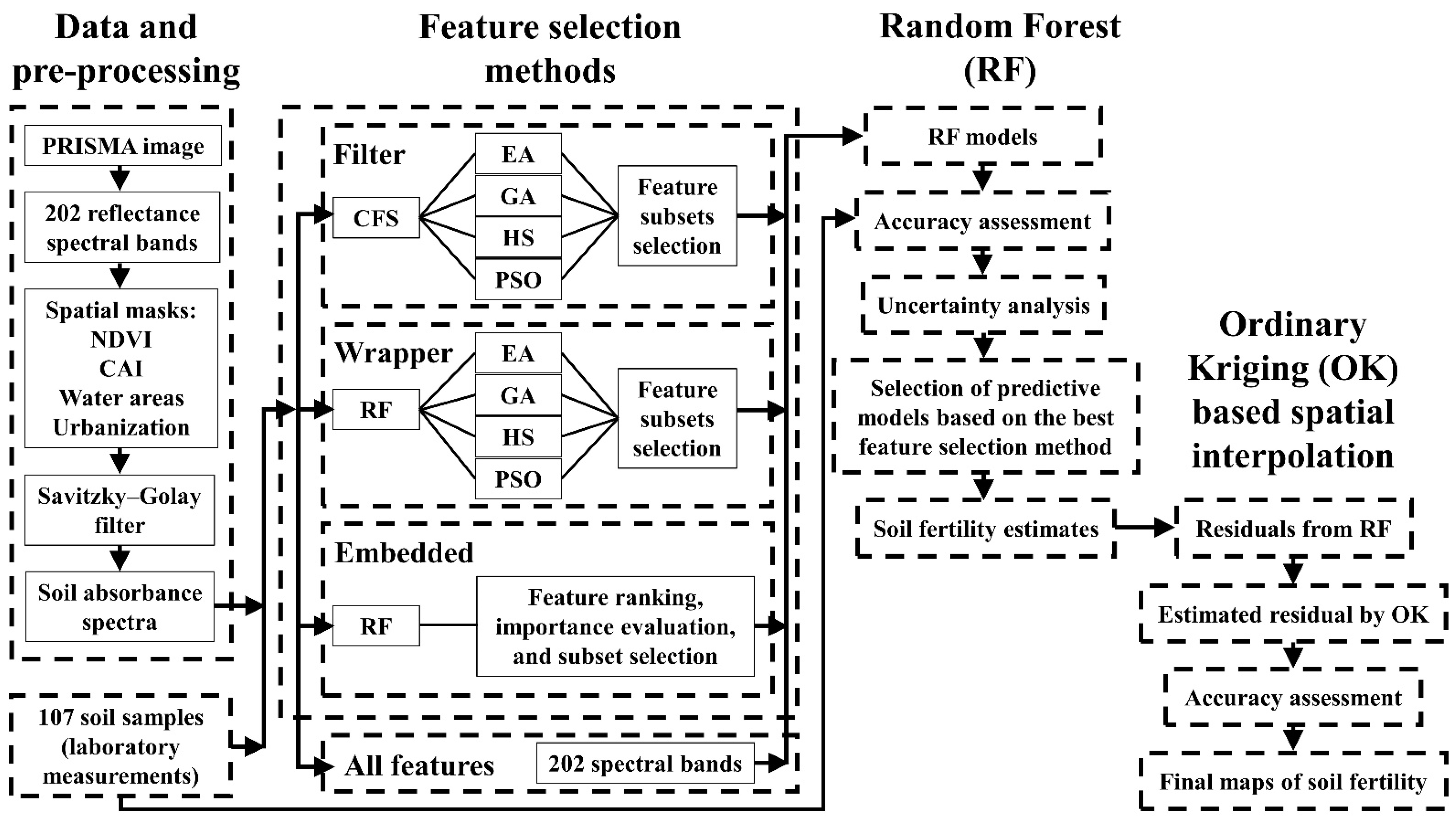
2. Materials and Methods

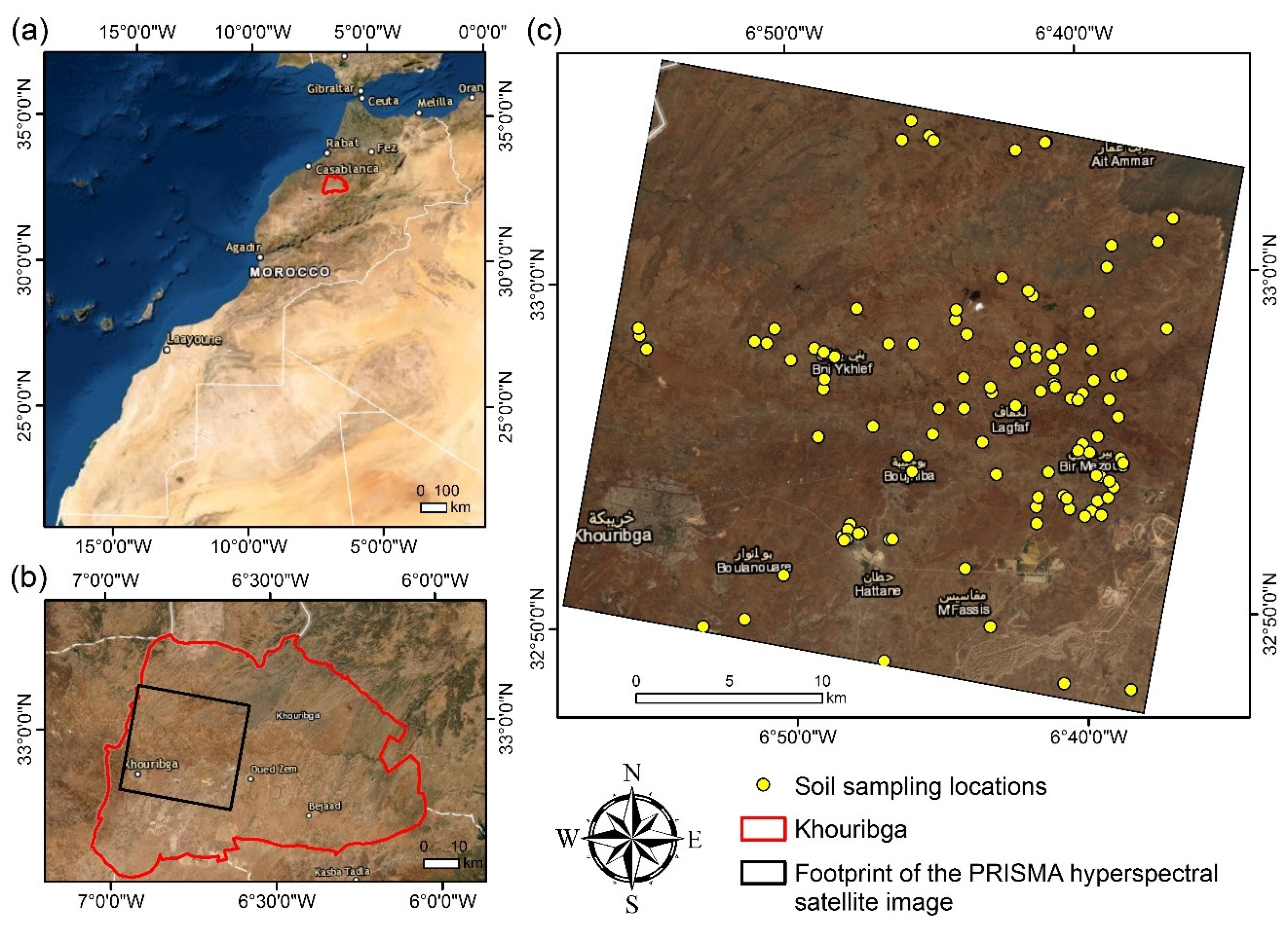
2.1. Study Area and Soil Dataset

The study area covers 950.55 km² within the province of Khouribga, northern Morocco (Figure 1). It is characterized by a semiarid climate with irregular rainfall, low average annual precipitation (350 mm), a high-temperature season, and a critical water deficit due to high evapotranspiration levels (1355 mm/y). This area is characterized by rolling land, with altitudes ranging from 0 to 963 m above sea level, and is mainly devoted to olive trees, orange trees, almond trees, and green plants. The primary parent materials are limestone, alluvium, phosphate sediment, marl, and siltstone. This geological complexity induced the formation of diverse soil types, such as Regosols, Calcaric Chernozems, Lithosols, and Rendzinas [40].

In September 2018, one hundred and seven soil samples were taken from 0–20 cm over the study area (Figure 1c). Each soil sample was made up of five sub-samples, and these five sub-samples were taken within a 10 × 10 m square centered on the geographical position of the sampling plot as recorded by a GPS instrument. Before being chemically analyzed, the soil samples were air-dried and sieved to 2 mm [41,42,43]. The organic matter content was measured by the Walkley Black oxidation method [44]. The available soil phosphorus (P₂O₅) and potassium (K₂O) contents were measured by inductively coupled plasma (ICP) [45].

2.2. PRISMA Hyperspectral Imagery

The PRISMA (PRecursore IperSpettrale della Missione Applicativa) is a hyperspectral satellite system launched by the Italian Space Agency (ASI) on 22 March 2019, into a low-Earth, sun-synchronous orbit at 615 km altitude, with a repeat cycle of 29 days and a revisit capability for a specific target of less than one week with off-nadir viewing. It is classified as a small satellite with a 5-year estimated operational life [46]. The instruments combine two hyperspectral sensors and one panchromatic camera. Two hyperspectral sensors can capture images in a continuum of 239 spectral bands ranging from 400 to 2500 nm, 66 in the VIS-NIR, and 173 in the SWIR spectrum, with a spectral resolution smaller than 12 nm and a spatial resolution of 30 m. The panchromatic camera has a GSD of 5 m and works in the spectral range of 400–700 nm. The recorded images were in an area of interest spanning from 180°W to 180°E longitude and 70°N to 70°S latitude [47].

One cloud-free PRISMA scene was successfully acquired over the study area on 2 September 2021. The hyperspectral image was obtained in an HDF5 file format with levels of preprocessing L2D (reflectance) products. The L2D PRISMA product is an atmospherically corrected image cube as executed by the standard processing chain set up by ASI for PRISMA. TOA spectral radiance was converted to spectral reflectance using a multidimensional LUT approach. MODTRAN-6 [48] based on several atmospheric models is used with a multi-scattering approximation to build a LUT for each band [47]. Values are stored in an array and indexed as a function of different geophysical values (summarizing various atmospheric scenarios) and observational (the so-called sun–target–satellite geometries) parameters. The LUT considers atmospheric models (mid-latitude winter and summer), geometric conditions (sun, relative azimuth angle, and view zenith angle), ground altitude, precipitable water vapor, and aerosol optical thickness [47].

2.3. Preprocessing

The PRISMA L2D cloud-free scene provided in HDF5 format was first transformed into ENVI format by the R package PRISMA-read [49], specifically designed to import and convert the PRISMA hyperspectral data. After the transformation, we removed from the resultant hyperspectral data (1) the spectral band B4 (at 402.46 nm) owing to noise in this band and (2) the spectral bands between 1338.95 and 1459.07 nm (between bands B41 to B52), as well as between 1793.69 and 1967.06 nm (band B85 to B104) owing to vibrational-rotational H₂O absorption bands. Therefore, a total of 202 PRISMA spectral bands were maintained.

The study area was covered by bare soil, urban activity, water, and vegetation consisting mainly of olive, orange, almond, and green plants. The following procedure was used to isolate the bare soil pixels from the PRISMA hyperspectral data. Pixels with normalized difference vegetation index (NDVI) and cellulose absorption index (CAI) [50] values over a threshold of 0.18 and 0.00 were masked, respectively. These values have been determined after considering different parcels. The NDVI values have been computed based on PRISMA bands at 660.28 nm and 833.78 nm. The CAI was calculated using PRISMA bands centered at 2000 nm, 2100 nm, and 2200 nm. Reflectance pixels values of less than 18% at 1666 nm have been masked to remove water areas. A visual examination was used to identify the urban areas, then masked. Finally, when the PRISMA hyperspectral data were taken (on 2 September 2021), bare soils covered 87% of the entire study site.

Before starting the modeling and mapping process on PRISMA hyperspectral data, a Savitzky–Golay with second-order polynomial smoothing was applied to reduce the signal noise. The reflectance (R) has been transformed into absorbance (A) (log [1/reflectance]) at each waveband to strengthen the spectral features [51]. Finally, the spectral wavebands significantly related to soil nutrients were investigated based on correlation analysis.

2.4. Hyperspectral Feature Selection

Hyperspectral data includes redundant information, which makes modeling difficult. The low number of samples compared to a large number of bands in the hyperspectral data can cause the Hughes phenomenon [52]. Therefore, feature selection or evaluation is essential to building models using hyperspectral remote sensing data. Feature selection is frequently used for numerous factors: (i) it enables the ML algorithm to be trained more quickly; (ii) it decreases the complexity of the model; and (iii) it makes interpretation easier [53]. Furthermore, when a suitable subset is selected, it increases the model’s accuracy and inhibits overfitting. Feature selection methods can be classified into three main groups: filters, wrappers, and embedding approaches [39].

Filter techniques are the most basic, quick, and general ways to select or assess the relevant features. They do not need a learning algorithm to rank and select features and feature subsets; instead, they use statistical metrics produced directly from the training data, such as correlation, distance, knowledge, reliance, and consistency. In this way, they attempt to allow just the most significant attribute to appear. Their principal limitation is that they fail to account for model prediction and feature interaction [54].

Wrapper techniques require a specific learning algorithm and rely on ML model prediction to select the optimal collection of features. The important features may be determined by generating a model with all the features and assessing them using an objective function, cross-validation, and performance as the criteria for evaluation. Generally, the wrapper technique outperforms the filter technique, although it is more computationally costly [55]. Nevertheless, they demand more computer resources than filter methods and must ultimately resort to search (e.g., stepwise search, genetic algorithm, particle swarm optimization algorithm, etc.).

Finally, the embedded methods can be defined as a feature ranking method incorporated into the learning process of the selected ML model. Embedded approaches are more computationally efficient than wrappers because they only use one model to deliver results. However, as a result, they are restricted to the biases and feebleness of a given ML model [54].

This study evaluated three feature selection techniques that covered the previously mentioned key categories, including correlation-based feature subset selection (CFS) [56] as filter methods, RF-wrapper, and RF-embedded methods (

Table 2. List of feature evaluators.

Feature Selection Approaches	Attribute Evaluation Methods	Search Methods	Feature Evaluation Results (Output)
Filter	Correlation-based Feature Subset Selection (CFS)	EA	Feature subset selection
		GA
		HS
		PSO
Wrapper	RF-Wrapper	EA	Feature subset selection
		GA
		HS
		PSO
Embedded	RF-Embedded	Ranked	Feature ranking

Notes: RF: random forest, EA: evolutionary algorithm, GA: genetic algorithm, HS: harmony search, and PSO: particle swarm optimization algorithm.

and Figure 2). The CFS and RF-wrapper methods have been based on different search approaches, such as the evolutionary algorithm (EA) [57], genetic algorithm (GA) [58], harmony search (HS) [59], and particle swarm optimization (PSO) algorithm [60]. We evaluated the methods by classifying them into two groups based on the feature assessment results (i.e., feature subset selection and feature ranking) (Table 2 and Figure 2). To be executed automatically, all feature selection methods were integrated into weka-packages using WEKA software, version 3.9.5 (The University of Waikato, Hamilton, NZ).

2.4.1. Filter Methods

The correlation-based feature subset selection (CFS) algorithm [56] is a filter approach that determines the usefulness of a subset of attributes by taking into account each feature’s unique predictive capacity as well as the degree of redundancy among them [56]. The feature subsets are assessed by increasing a feature subset’s reliance on the target class while reducing intercorrelation within the subset. In our study, search strategies based on EA, GA, HS, and PSO algorithms were employed to explore the potential feature subsets.

2.4.2. Wrapper Methods

The wrapper method was used in this work to evaluate the subset of hyperspectral bands and to find the optimum feature subset. A learning scheme was implemented for the wrapper method to assess attribute sets, and the learning scheme’s accuracy was calculated using all the training data to find the optimal subset. As a result, the features that produced maximum accuracy were identified as the optimum feature subset. Since RF models were used as the regression method evaluated in this study (see Section 2.5), we examined four wrapper search methods (i.e., EA, GA, HS, and PSO algorithms). Thus, these learning schemes were set to RF regression models to get the highest possible feature subsets performance (Table 2 and Figure 2). For the wrapper feature selection methods, the weka.attributeSelection function with the class weka.attributeSelection. WrapperSubsetEval assessed attribute sets using a learning scheme with all training data and based on the performance measure. The RF-based wrapper methods were trained with optimal parameters in the WEKA classifier package.

2.4.3. Embedded Methods

Embedded methods interact with models to rank features. According to [35], the feature evaluation and ranking approach based on the RF is referred to as an embedded technique, which computes the mean decrease in accuracy (MDA) using bagging iterations to offer criteria of variable importance for each feature [61]. During the training step, MDA uses the RF’s ability to evaluate a feature’s influence on model accuracy to generate feature rankings [62].

Afterward, features with zero or almost zero contribution to the modeling are removed. Feature subset selection using RF regression can be achieved by examining feature rankings in descending order of nested RF models, keeping the most miniature and most accurate model. Generally, if adding a feature results in only a minor or no reduction in model error, the mentioned feature is then removed. The process concludes by generating a list of the most discriminating features, constituting the subset of the selected features.

2.5. Predictions of Soil Nutrients Contents

After selecting the most important features from the hyperspectral data, the feature selection methods were evaluated by applying the RF regression algorithm to the optimized datasets in order to predict the soil nutrient content (Figure 2). The soil samples were randomly partitioned into training (75%) and validation (25%) sets, using the split function in the WEKA software. The RF regression algorithm was trained with the training dataset, and the trained model was validated in the testing stage.

The RF algorithm has been extensively used in the remote sensing field due to its high performance and efficiently handling of big and highly dimensional datasets [63]. It is well-known in the remote sensing community, and several studies have evaluated its applicability [64]. RF algorithm implements many decision tree classifiers to categorize an input vector by casting a single vote for the most common class [65]. The bagging approach generates a random subset taken from the training sample set to develop each tree. Unlabeled items are classified by allocating them to the most frequently voted class. The RF needs two parameters to build the predictive model: the decision tree number (ntrees) and the number of randomly selected predictors at each tree node (mtry) [66]. A new dataset is predicted by sending each case of the dataset down to each growing tree. Then, the forest selects the class with the highest vote from the trees for that case [67]. The trees.RandomForest package in WEKA software was used to realize the RF regressions and the parameters of the model were selected based on multisearch-weka-package.

2.6. Uncertainty Analysis

A bootstrapping technique [65] was employed in this study to measure the uncertainty of the soil nutrient prediction models, described in Section 2.5. All soil samples were randomly split between training (75%) and validation (25%) for each iteration of the bootstrap uncertainty analysis to train 50 distinct RF models. Based on the validation data, the goodness-of-fit statistics parameters were calculated for each bootstrap iteration, determining the mean and standard deviation for each goodness-of-fit statistic throughout the bootstrap process. The RandomSplitResultProducer and RegressionSplitEvaluator functions in WEKA software, version 3.9.5 (The University of Waikato, Hamilton, New Zealand) were used to realize the uncertainty analysis.

2.7. Kriging Method

The kriging method [68] is a spatial interpolation approach frequently applied for soil attribute quantification [69,70]. It is presumptively possible to treat the interpolated parameter as a regionalized variable. The hypothesis is that a regionalized variable varies continuously from one site to the next. As a result, points close to each other have some spatial correlation, whereas ones far apart are statistically independent. The kriging technique’s variogram describes this assertion as an estimator of variance dispersed across sample sites [71]. The variogram is a graph of sample semivariance (y-axis) vs. lag distance (distance between sample sites, x-axis). The experimental variogram can be generated using either measured or estimated samples.

The kriging method includes five operation steps. In the first step, the data were examined and imported as the input data (layer). The second step involves choosing the kriging type. The third step consists of adjusting the semivariogram models. A goal with kriging is to select a model that “fits” the scatter of points. The interpolation is the fourth step. Kriging interpolation weights the surrounding measured values to derive a prediction for an unmeasured location. The fifth step involves the evaluation of the accuracy of the prediction results [70].

In this work, the ordinary kriging technique was applied for the spatial interpolation of the map’s values obtained from PRISMA hyperspectral data and based on the best soil nutrient prediction models (Figure 2). Various models were evaluated to fit the experimental variogram, such as circulaire, spherique, tetraspherical, pentaspherical, exponential, Gaussian, rational quadratic, hole effect, k-bessel, j-bessel, and stable models. Spatial maps of soil nutrients (i.e., SOM, available soil P₂O_5, and K₂O) were produced with ArcMap 10.8 [72] and its geostatistical analyst plugin.

2.8. Assessment of Model Performances

Five goodness-of-fit parameters were calculated to evaluate the RF models’ performance in the validation sets: the coefficient of determination ($R_{val}^2$), the root mean square error (RMSEP), the mean absolute error (MAEP), bias, and the ratio of performance to interquartile (also known as RPIQ, the ratio of the interquartile to the RMSEP; that differed from RPD, the ratio of the standard deviation to RMSEP) [73]. The performance of the models integrated into the OK procedure was evaluated, and the best model was selected based on the minimum values of nugget effect, RMSE, and average standard error (ASE) of cross-validation. The nugget effect value described the spatial variability of the residuals and their dependency on the soil nutrient content [30]. After predictions and performance assessments of OK models, the best models were selected and evaluated in the validation sets using $R_{val}^2$, RMSEP, MAEP, bias, and RPIQ parameters.

3. Results

3.1. Descriptive Statistics for Soil Nutrients

Descriptive statistical analysis of the SOM, available soil P₂O_5, and K₂O contents was carried out based on the 107 samples (

Table 3. Statistics of soil nutrients (SOM in %, available soil P₂O_5, and K₂O in ppm) in the study area.

Soil Nutrients	Min	Max	Mean	SD	IQ	Sk	CV
SOM	1.97	4.40	3.09	0.54	0.77	−0.03	17.44
P2O5	3.00	254.76	52.82	45.04	46.00	2.54	85.25
K2O	39.16	1067.00	291.73	203.26	214.5	1.74	69.67

Notes: number of soil samples (n = 107); SD: standard deviation; IQ: inter-quartile distance; Sk: skewness; CV: coefficient of variation (%).

). The concentration of OM in soil samples varied between 1.97 and 4.40%, with a mean and standard deviation of 3.09 and 0.54%, respectively. The soil P₂O₅ range varied between 3.00 and 254.76 ppm and soil K₂O between 39.16 and 1067.00 ppm. The mean values of soil P₂O₅ and K₂O were 52.82 and 291.73 ppm, respectively. For every soil nutrient, the coefficient of variation (CV) was greater than 17% in all cases, showing that the datasets were heterogeneous. The highest CV value was found in the soil P₂O₅ content, indicating that P₂O₅ was the most heterogeneous fraction in this region (Table 3). Soil nutrient contents have a considerable variation and standard deviation, which might help build an accurate model. The mean variation of soil nutrients in the datasets was high and equal to 57.45%.

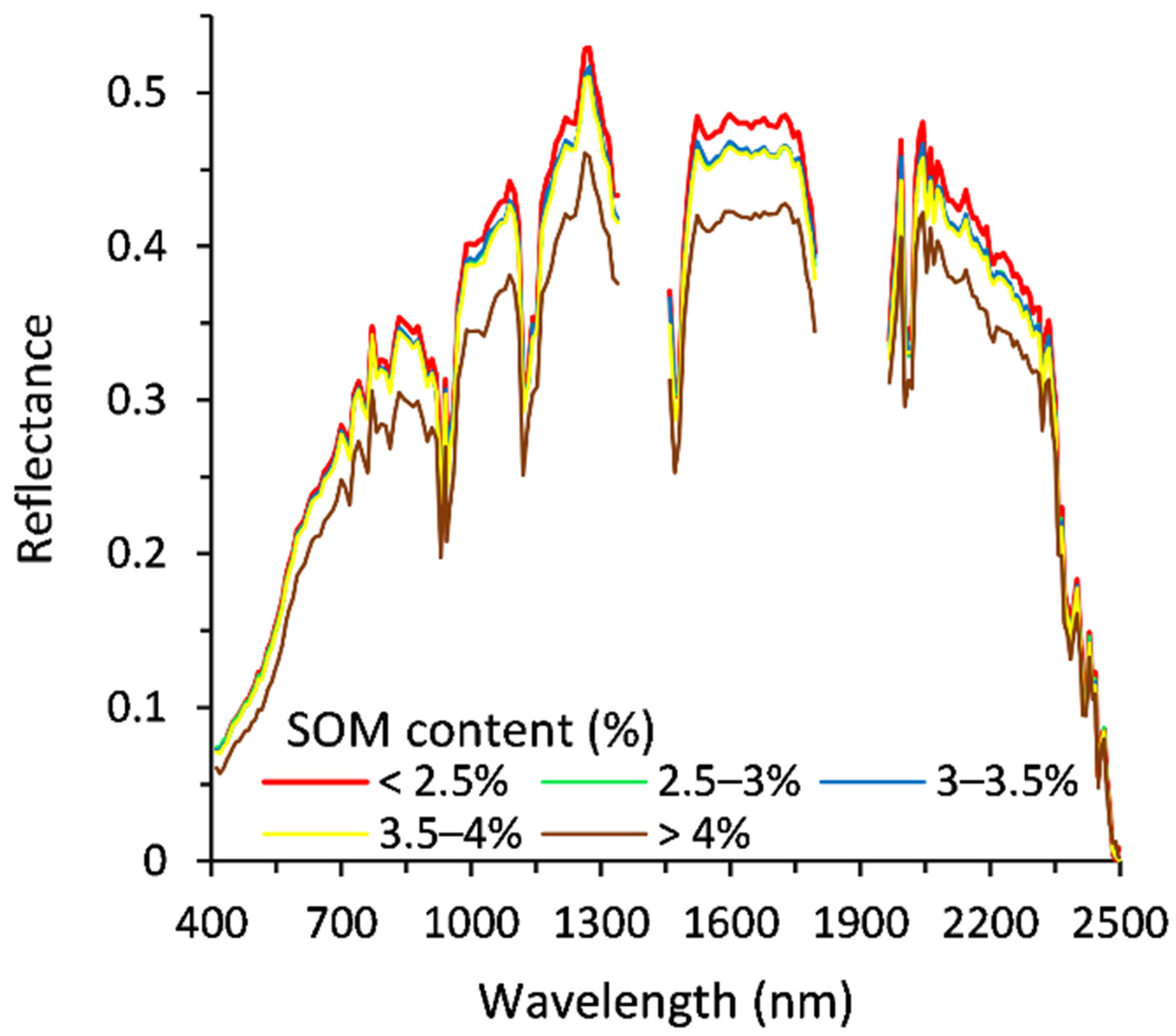
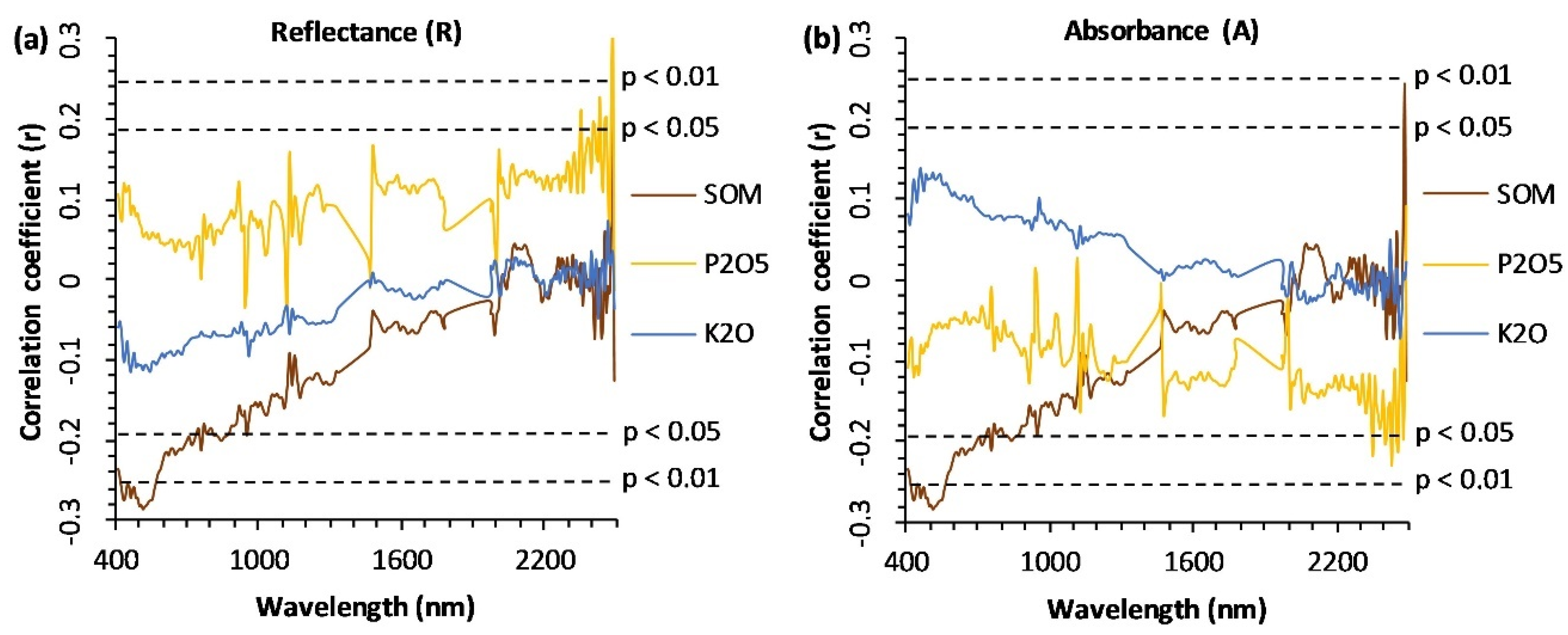
3.2. Pretreatment Process and Correlation Analysis

The PRISMA hyperspectral data of soil samples (Figure 3) showed that the shapes of reflectance were similar to those of soil samples in other studies (e.g., [28,74,75]). The spectral curves had absorption bands removed at 1400 and 1900 nm; these bands are related to the presence of hydroxide (OH) in free water (H₂O molecules) [76]. The most common sensitive bands associated with clay minerals are those at 1400–1410 nm and 2160–2200 nm due to the metal–OH band plus the O–H stretch combination and C–O [77]. SOM has broad sensitive bands from the VIS to SWIR range (400–2500 nm) due to the overtones and combination absorptions of O–H, C–H, and N–H bonds [78]. The spectral bands of soil N, P, and K are indirectly associated with the vibration modes of functional groups, such as OH⁻, SO₄²⁻, CO₃²⁻ and their combinations [16].

The mean hyperspectral reflectance curves of soil samples with five different classes of SOM content are illustrated in Figure 3; overall spectral reflectance increases as the SOM content decrease. The SOM content of less than 2.5% and more than 4% correspond to the highest and lowest reflectance, respectively. The PRISMA hyperspectral reflectance fluctuation scheme remains almost similar regardless of the SOM content (Figure 3).

3.3. Pretreatment Process and Correlation Analysis

The coefficient of correlation was calculated between each soil nutrient’s content and the PRISMA spectral formats as the reflectance (R) and absorbance (A) in the wavelength range between 400 and 2500 nm (Figure 4 and

Table 4. Correlations (r) between two PRISMA spectral formats (reflectance (R) and absorbance (A)) and soil nutrient contents.

Soil Nutrients	R			A
	/rmin/	/rmax/	n	/rmin/	/rmax/	n
SOM	−0.285 1	0.239 1	51	−0.063	0.309 1	53
P2O5	−0.037	0.317 1	8	−0.229 1	0.091	7
K2O	−0.114	0.073	0	−0.071	0.138	0

n = the number of attuned bands. rmin = minimum correlation coefficients. rmax = maximum correlation coefficients. ¹ Significant correlation (−0.191 ≥ r ≥ 0.191, p < 0.05).

). Significant correlations between R values and SOM contents occurred at 51 spectral bands (r > 0.191, p < 0.05). Significant correlations between R values and soil P₂O₅ contents were observed at 8 spectral bands. The R values and soil K₂O contents did not show any significant correlation. Similarly, substantial correlations between A and SOM occurred at 53 spectral bands. Significant correlations between A values and soil P₂O₅ contents were observed at 7 spectral bands. No significant correlation was found between A and soil K₂O contents. The highest number of bands correlated with soil nutrient content was obtained by PRISMA absorbance spectra (Figure 4 and Table 4).

3.4. Performance of Feature Selection Methods

Feature selection methods were applied to find accurate hyperspectral wavebands for predicting the soil nutrient content. The RF regression models were generated with each feature selection method to predict the SOM, available soil P₂O_5, and K₂O content. These methods were then assessed using goodness-of-fit parameters. Next, the optimal RF models based on the best feature selection method were applied to all the bare soil pixels of the PRISMA image to elaborate estimated SOM, available soil P₂O_5, and K₂O content maps.

Because of the diverse result outputs from the feature selection methods, the comparison of the advantages in terms of prediction accuracy was separated into three sections, i.e., (i) using all features, (ii) the optimal feature subset derived by each feature–subset–evaluation method, and (iii) the ranked feature list derived by the feature–importance–evaluation method.

3.4.1. Evaluation of All Features

Using all hyperspectral wavebands, the RF models provided a weak $R_{val}^2$ concordance and a high RMSEP to predict the soil nutrient content. The RF model of SOM had the highest accuracy, with an $R_{val}^2$ of 0.41, an RMSEP of 0.46%, an MAEP of 0.36%, a bias of −0.02, and an RPIQ of 1.86. For the soil K₂O content, the results showed an $R_{val}^2$ of 0.17, an RMSEP of 205.64 ppm, an MAEP of 136.62 ppm, a bias of −48.01, and an RPIQ of 1.03. However, the minimum goodness-of-fit statistics values were observed for the soil P₂O₅, with an $R_{val}^2$ of 0.09, an RMSEP of 56.19 ppm, an MAEP of 32.49 ppm, a bias of −5.70, and an RPIQ of 0.59, respectively.

3.4.2. Evaluation of Subset Selection Methods

From the 202 hyperspectral wavebands, the CFS- and RF-wrapper-based search methods selected different numbers of effective spectral bands in predicting soil nutrient content (

Table 5. Performance comparison of feature subset selection methods based on soil nutrients prediction accuracy.

Soil Nutrients	Attribute Evaluation Methods	Search Methods	Bands Selected	${\mathit{R}}_{\mathit{v}\mathit{a}\mathit{l}}^{\mathbf{2}}$	RMSEP	MAEP	Bias	RPIQ
SOM	CFS	EA	3	0.02	0.63	0.53	0.04	1.38
		GA	57	0.39	0.48	0.38	−0.01	1.82
		HS	22	0.34	0.49	0.40	−0.01	1.76
		PSO	33	0.34	0.49	0.40	−0.02	1.75
	RF-Wrapper	EA	70	0.43	0.45	0.35	−0.04	1.90
		GA	69	0.47	0.44	0.34	−0.06	1.96
		HS	38	0.37	0.48	0.36	−0.06	1.80
		PSO	63	0.43	0.46	0.35	−0.04	1.90
P2O5	CFS	EA	48	0.09	55.97	33.10	−4.86	0.59
		GA	47	0.06	57.03	33.39	−5.77	0.58
		HS	36	0.02	58.89	34.27	−7.71	0.57
		PSO	32	0.02	58.46	34.26	−5.31	0.57
	RF-Wrapper	EA	74	0.08	56.06	32.60	−6.12	0.58
		GA	88	0.10	55.90	32.02	−5.60	0.60
		HS	28	0.04	57.59	34.13	−5.27	0.58
		PSO	46	0.05	57.41	32.85	−5.50	0.58
K2O	CFS	EA	1	0.17	205.71	162.42	−40.84	1.03
		GA	58	0.18	205.03	135.40	−41.74	1.03
		HS	20	0.14	209.82	137.37	−37.45	0.99
		PSO	35	0.08	217.27	138.05	−40.62	0.97
	RF-Wrapper	EA	75	0.19	203.11	131.52	−47.66	1.04
		GA	73	0.19	203.83	131.47	−47.84	1.04
		HS	38	0.19	203.05	126.51	−49.01	1.04
		PSO	43	0.20	202.07	128.88	−48.15	1.05

Notes: CFS: correlation-based feature subset selection, EA: evolutionary algorithm, GA: genetic algorithm, HS: harmony search, and PSO: particle swarm optimization algorithms. SOM in %, available soil P₂O₅ and K₂O in ppm for the RMSEP and MAEP values, respectively.

). Generally, the features selected by the RF-based wrapper methods provided superior prediction accuracy than the features selected by the CFS methods or the use of all features. Furthermore, the GA–RF wrapper-based feature selection method picked the most sensitive features compared to other subset selection methods. It showed the highest soil nutrient prediction accuracy, with an $R_{val}^2$ mean value of 0.25 (Table 5).

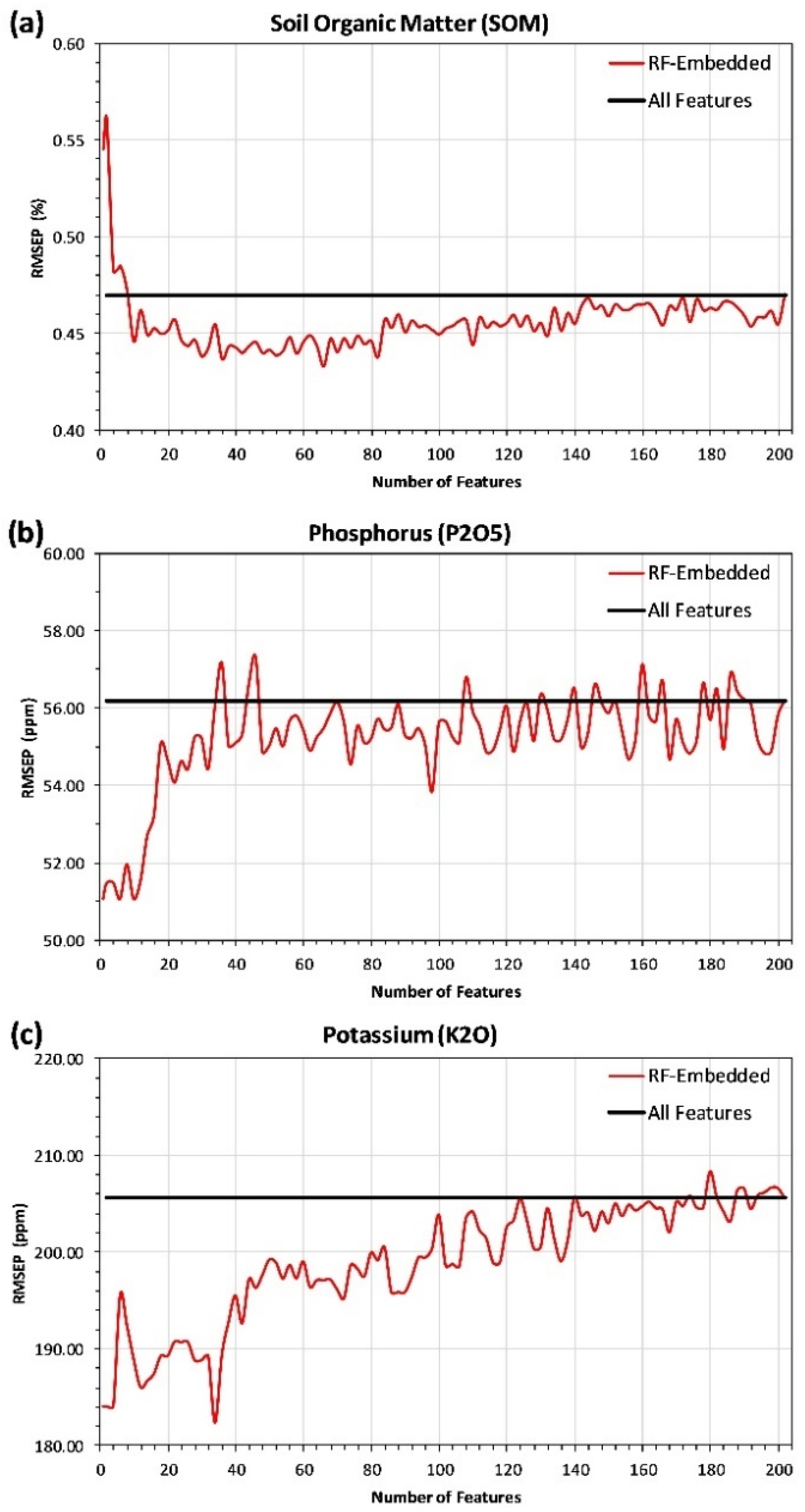
3.4.3. Evaluation of Feature Ranking Methods

The RF models accuracy varies according to the number of selected wavelength bands (spectral channels). To assess trends, the RMSEP was computed for each collection of features, beginning with the first and incrementing by one until a model containing all variables was found. Figure 5 shows the RMSEP variability based on feature rankings of the RF-embedded technique, which was used to estimate the soil nutrient content. The RF-embedded models attained smaller RMSEP values, with minimum feature subsets, compared to models including all features (Figure 5). In detail, for the SOM, available soil P₂O_5, and K₂O, the RF-embedded models exposed the lowest RMSEP values of 0.43%, 51.07 ppm, and 182.31 ppm, at 66, 9, and 34 features, respectively. As expected, the best feature selection method was the RF-embedded as it reached the maximum accuracy ($R_{val}^2$ = 0.5, 0.26, and 0.36; MAEP= 0.33%, 29.98 ppm, and 126.39 ppm; bias = −0.04, −5.32, and −53.02; RPIQ = 2.02, 0.65, and 1.16, for SOM, available soil P₂O₅ and K₂O, respectively). This result also showed the greatest accuracy achieved across all the feature selection techniques investigated in this study (Table 5 and Figure 5). Finally, significant improvements were reached by applying RF-embedded or RF-wrapper-based feature selection methods compared to the use of all features (Table 5 and Figure 5).

Figure 6 presents the wavelengths of the important bands derived from the best feature selection method (i.e., RF-embedded). As indicated in the preceding paragraph, these wavebands had the greatest influence on the predictive performance of the SOM, available soil P₂O_5, and K₂O content. The VNIR (400–1100 nm) and SWIR (1481–1756 nm and 2103–2435 nm) wavelengths were found to be important in predicting SOM (Figure 6). The selected wavelengths for the P₂O₅ were 434, 951, 988, 1038, 1185, 1765, 2276, 2313, and 2435 nm. For the K₂O, the selected wavelengths focus on band information from the VNIR (Figure 6).

3.5. Model Uncertainty Analysis

The predicted models’ uncertainty must be quantified in order to confirm their relevance for soil fertility mapping and providing agricultural fertilization recommendations. This uncertainty may be assessed by comparing the goodness-of-fit statistics from the bootstrap aggregate (

Table 6. Mean and standard deviations of goodness-of-fit statistics values calculated from the RF models of SOM, available soil P₂O_5, and K₂O content with 50 bootstrap iterations.

Soil Nutrients	Attribute Evaluation Methods	Search Method	Bands Selected	RMSEP	MAEP
SOM	All Features	-	202	0.44 (0.04)	0.36 (0.04)
	CFS	EA	3	0.51 (0.05)	0.42 (0.05)
		GA	57	0.45 (0.05)	0.36 (0.05)
		HS	22	0.46 (0.05)	0.37 (0.04)
		PSO	33	0.45 (0.04)	0.36 (0.04)
	RF-Wrapper	EA	70	0.43 (0.04)	0.34 (0.04)
		GA	69	0.43 (0.04)	0.34 (0.04)
		HS	38	0.43 (0.04)	0.34 (0.04)
		PSO	63	0.43 (0.04)	0.34 (0.04)
	RF-Embedded	ranked	66	0.43 (0.04)	0.35 (0.04)
P2O5	All Features	-	202	45.86 (11.25)	32.52 (5.83)
	CFS	EA	48	45.49 (10.79)	32.07 (5.73)
		GA	47	46.23 (11.37)	32.49 (5.98)
		HS	36	46.77 (10.86)	33.10 (5.61)
		PSO	32	45.27 (11.32)	31.96 (5.86)
	RF-Wrapper	EA	74	44.41 (11.54)	31.50 (5.97)
		GA	88	44.65 (11.34)	31.81 (5.84)
		HS	28	44.14 (11.27)	30.92 (5.91)
		PSO	46	44.22 (11.56)	31.41 (5.89)
	RF-Embedded	ranked	9	43.69 (10.36)	31.16 (5.38)
K2O	All Features	-	202	196.25 (45.67)	141.63 (26.54)
	CFS	EA	1	239.22 (45.34)	174.71 (29.41)
		GA	58	186.74 (48.20)	133.32 (25.61)
		HS	20	186.15 (49.33)	135.82 (25.45)
		PSO	35	183.86 (46.17)	132.45 (24.91)
	RF-Wrapper	EA	75	189.80 (44.48)	137.56 (25.96)
		GA	73	185.64 (47.89)	132.87 (26.72)
		HS	38	183.60 (45.10)	130.90 (26.09)
		PSO	43	181.00 (44.71)	130.43 (25.54)
	RF-Embedded	ranked	34	186.45 (41.47)	134.81 (24.89)

Notes: CFS, correlation-based feature subset selection, EA: evolutionary algorithm, GA: genetic algorithm, HS: harmony search, and PSO: particle swarm optimization algorithms. The numbers in the brackets are standard deviations of 50 iterations. SOM in %, available soil P₂O_5, and K₂O in ppm for the RMSEP and MAEP values, respectively.

) with the goodness-of-fit statistics from all models (Table 5 and Figure 5). Each model uncertainty was computed from the 50 bootstrapping iterations (Table 6). The goodness-of-fit statistics results from the bootstrap approach (Table 6) compared to the initial models (Table 5 and Figure 5) indicate that the RF models fit statistics differed minimally, implying that the models had little variability and uncertainty. For example, the best SOM model (i.e., RF-embedded) had an MAEP of 0.33%, whereas the bootstrap uncertainty results produced an MAEP of 0.35%, with a standard deviation of 0.04% (Table 6).

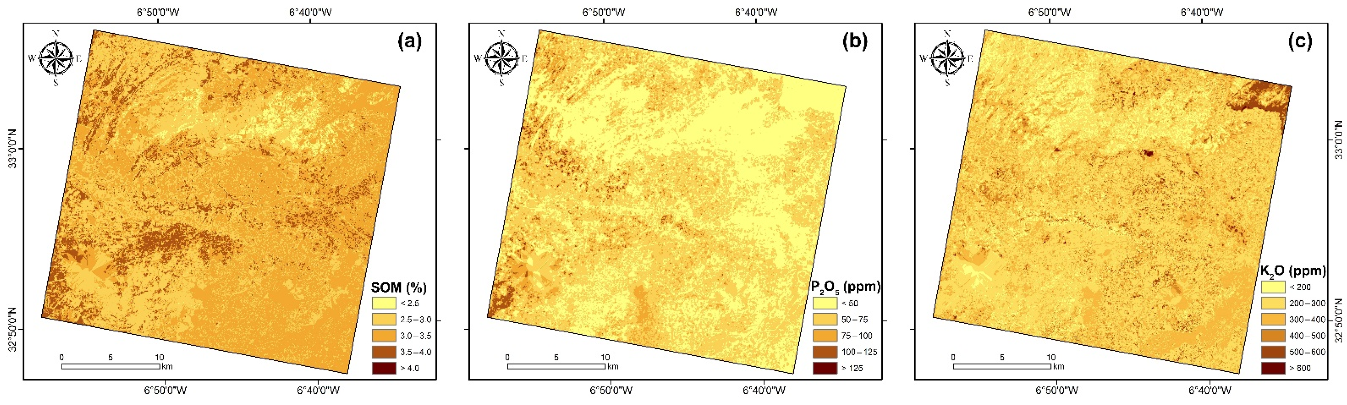
3.6. Spatial Prediction of Soil Nutrients by RF-OK Models

In the first stage, the best models based on PRISMA spectra (described in Section 3.4.3) were applied to all bare soil pixels included in the PRISMA image to produce the soil nutrient maps within the Khouribga area at 30 m of spatial resolution. In the second stage, the OK approach was used to interpolate all values retrieved from each soil nutrient map in order to estimate new values within all pixels of the PRISMA image. The exponential models were selected based on the minimal nugget effect, RMSE, and ASE values of cross-validation, after evaluating eleven function models during semi-variogram modeling using ArcGIS software.

Table 7. Semi-variogram results of soil nutrients estimated residuals by RF-OK models.

Model	Soil Nutrient	Range (m)	Nugget	Sill	Nugget Effect	RMSE	ASE
Exponential	SOM	258.24	0.00	0.06	0.00	0.11	0.12
	P2O5	360.00	126.15	293.81	42.94	11.84	13.23
	K2O	242.32	1119.11	5877.16	19.04	48.12	51.92

shows the semi-variogram parameters of the RF-OK models for the soil nutrients. The nugget effect was used to characterize the spatial variability and dependency of the soil nutrient contents. If it was less than 25%, the variable was regarded as extremely spatially dependent; if it was between 25 and 75%, the variable was considered as moderately spatially dependent; and if it was more than 75%, the variable was considered as weakly spatially dependent [79]. In this study, the nugget effect of the residuals estimated from the RF-OK models exhibited high spatial dependence for the SOM (0.00%) and soil K₂O (19.04%) and moderate spatial dependence for the soil P₂O₅ (42.94%) (Table 7). Moreover, based on the independent validation set, the RF-OK residuals demonstrated higher goodness-of-fit statistics values for the soil nutrients compared to only RF residuals, with the highest $R_{val}^2$ values for SOM (0.69), soil P₂O₅ (0.44), and K₂O (0.51), respectively (

Table 8. Goodness-of-fit statistics values of the RF-OK models at the validation set for the soil nutrients.

Soil Nutrients	${\mathit{R}}_{\mathit{v}\mathit{a}\mathit{l}}^{\mathbf{2}}$	RMSEP	MAEP	Bias	RPIQ
SOM	0.69	0.34	0.27	0.02	2.56
P2O5	0.44	44.10	27.52	−1.21	0.75
K2O	0.51	158.29	99.28	−19.54	1.34

Notes: SOM in %, available soil P₂O₅ and K₂O in ppm for the RMSEP and MAEP values, respectively.

).

For this study, the RF-OK models were selected to produce the SOM, available soil P₂O_5, and K₂O maps from the hyperspectral remote sensing data (Figure 7) since they had the best predictive performance and the highest fitting ability for the soil nutrient spatial variability (Table 8). The soil nutrient maps showed high concentrations of SOM and soil P₂O₅ in the northwest and southwest parts and high soil K₂O concentrations in the northeast part, whereas the lower concentrations were exposed in the north, northeast, and southwest for SOM, soil P₂O_5, and K₂O, respectively. Based on the soil nutrient maps, the relationship between organic matter, phosphorus, and potassium contents in the soil can be explored spatially. If the soils were high in organic matter, the amounts of phosphorus and potassium were especially low to middling. Thus, these maps followed pedological patterns and provided a spatially continuous surface mapping of the soil landscape. The southern part was characterized by the presence of very dark carbonate humus soils, clayey Rendzina soils, and stony crust in association with chernozem soils or red-brown soils developed on the weathering products of Cretaceous rocks. Furthermore, we frequently found bare and stony limestone areas crusted with eroded soil. However, the northern part was characterized by the presence of the podzolic soil, often eroded skeletally on deep ravine slopes, Chernozem soils, and dark brown soils of the plateaus formed on Permo-Triassic sedimentary rocks and red “Hamri”-type soils.

4. Discussion

4.1. Preprocessing Process

In this study, before spectral feature selection and soil nutrients modeling, the Savitzky–Golay filter was used to smooth and remove random noise from the PRISMA spectra. This filter was used in the most current studies combined or not with other methods to obtain an optimal pretreatment method proven to produce good results (e.g., [23,80]). For example, [81] employed only the Savitzky–Golay filter as an appropriate pre-processing method to improve the estimation accuracy for soil carbon.

The pre-processing based on the conversion of reflectance spectra (R) to absorbance (A) was evaluated in this study using correlation analysis between spectral wavebands and soil nutrient contents. The highest correlation was achieved using hyperspectral absorbance spectra (Figure 4 and Table 4). This finding agrees with earlier research [29,30,82]. According to the results of [82], the combination of the Savitzky–Golay filter and the conversion into absorbance (A) assist feature selection methods in selecting the informative variables and help yield good accuracy.

4.2. Effect of the Feature Selection Methods

In order to reduce the large dimensionality of the hyperspectral data and save computation time, spectral waveband selection may be more efficient than using a full spectrum for the quantitative model [83]. The results of this study revealed that feature selection techniques might help to reduce the dimension of PRISMA hyperspectral remote sensing data and could improve the prediction accuracy by up to 19%, depending on the used feature selection approach. Particularly, RF models’ performance appeared to significantly increase when only the optimum features were selected with feature selection techniques, such as the RF-wrapper or RF-embedded techniques. These results are consistent with the prior research, which concluded that selecting an adequate feature selection method can improve the ML algorithms’ performance when used for regression or classification problems [25,54,83]. Generally, the extraction of the optimum feature subsets from the RF-embedded method was the most consistent technique with the RF-regression method compared to CFS or RF-wrapper-based feature selection methods. Furthermore, the prediction accuracy may be influenced by two factors: the dataset’s sample size and the attribute evaluation methods [54].

Further research should investigate the application of additional feature selection techniques, such as Boruta algorithm [84], recursive feature elimination (RFE) [85], tabu search algorithm [86], and regularized random forests [87], as well as the feature importance estimated from boosting models, such as Xgboost [88] or AdaBoost [89]. Moreover, alternative implementations of popular predicted models, such as support vector machines (SVMs) [90], and artificial neural networks (ANNs) [91], should be examined to understand relative feature importance.

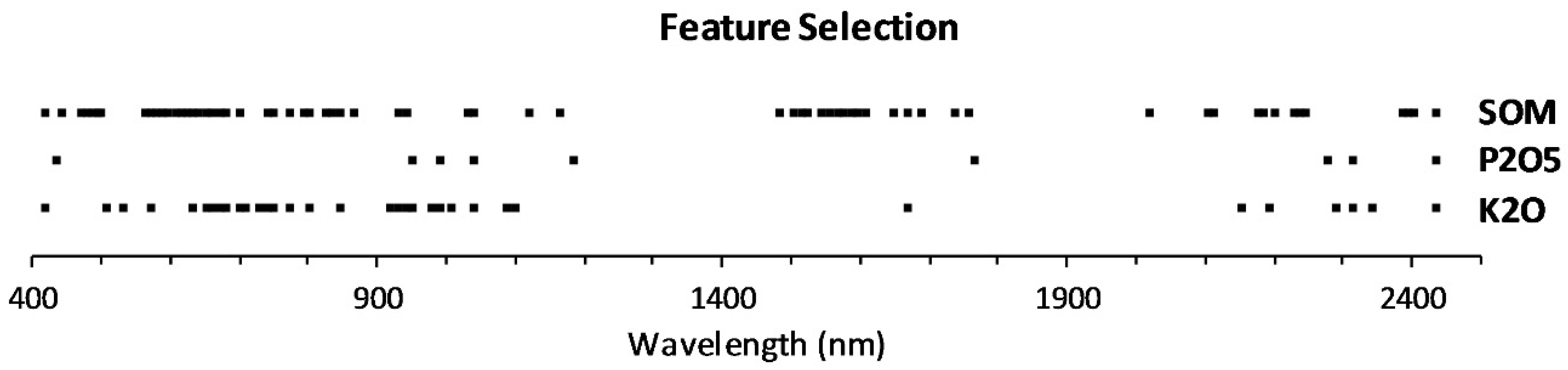
4.3. Feature Wavelengths

Several soil properties (e.g., soil clay or organic matter) can establish a direct relationship with the content at a specific spectral wavelength. For example, the SOM has broad sensitive bands from the VIS to the SWIR range (350–2500 nm) associated with the overtones and combination absorptions of O-H, C-H, and N-H bonds [78]. In this paper, the important wavelengths selected for the SOM ranged from 400–1100 nm, 1481–1756 nm, and 2103–2435 nm (Figure 6). Some of these wavelengths were consistent with those selected in existing studies, e.g., [25,92,93,94]. In [95], spectral features identified as important for SOC fell mostly within the range of 1000–1100 nm, 1200–1650 nm, 1880–1920 nm, and 2100–2320 nm.

Soil P and K need to rely on an indirect inversion of other soil component contents because they do not have any obvious spectral feature and usually exist in low concentrations in the soil [80]. The changes in the spectral profile can be due to indirect effects of the association of soil P and K with other elements that present a direct spectral response [25]. The feature wavelengths of the soil K in the VNIR region are mainly related to ferrihydrite, goethite, amine (N-H), organic matter, free water (O-H), cellulose, lignin, starch, and the first overtone of O-H stretch, Al-OH, or Mg-OH, among others. The components corresponding to the wavelength selection of soil P are similar to those of soil K, and the element types are complex and inconsistent [25]. In this work, based on RF model-fitting capabilities, the most sensitive wavelengths associated with soil P₂O₅ were 434, 951, 988, 1038, 1185, 1765, 2276, 2313, and 2435 nm. For K₂O, the key bands were included in the VNIR (400–1100 nm) wave range. Numerous studies have revealed that soil nutrients in these wavelengths have an important impact [25,30,34].

4.4. Prediction of Soil Nutrients by RF Models

The RF method based on the optimal subsets of hyperspectral features was used to predict soil nutrient content, which led to a moderately useful model for SOM ($R_{val}^2$ equal to 0.5) and low effectiveness for available soil P₂O₅ and K₂O ($R_{val}^2$ equal to 0.26 and 0.36, respectively) (described in Section 3.4.3). The RF models’ performance suggests that the relationships between SOM, available soil P₂O₅ and K₂O values, and spectral wavelengths were nonlinear in this study. Previous studies obtained similar results, e.g., [28,30,34]. The authors of [28] estimated the SOC content by Hyperion data in an Australian region and obtained an $R_{val}^2$ of 0.51 and an RPD of 1.43. HJ-1A hyperspectral imager (115 bands) was used by [30] to predict the available soil P and K content in China. The results showed R² and RMSE values for soil P of 42.91% and 40.80 ppm, respectively, and values for soil K of 48.53% and 67.46 ppm, respectively. In another study, total soil K and P content were mapped using HJ-1A HSI data with RMSE values of 20.37% and 34.71%, respectively [34]. The prediction of SOM and available P and K in soils by [24] using Landsat-8 OLI images showed quite satisfactory results, where R² values were 0.7, 0.68, and 0.55, respectively. Nevertheless, the soil nutrient prediction accuracy may differ from one study to another.

Discrepancies in these results can be attributed to various factors, including research methodology, measurements, locations, model performance, and data quality [96,97]. The remote sensing image with 30 m of spatial resolution can present mixed surfaces [98] that influence the spectral features of soil nutrients. Moreover, the amount of soil samples with a wide range of concentrations is also important, particularly in ML prediction models, which can cause a slightly diminished accuracy, especially in the validation step [99]. Thus, the bootstrap uncertainty analysis results can assist the interpretation of the models’ accuracy (Table 6).

4.5. Prediction of Soil Nutrients by RF-OK Models

In this study, the best performance was obtained using RF-OK models, giving the highest $R_{val}^2$ and RPIQ, with the lowest RMSEP and MAEP (Table 8). In comparison to a single nonlinear RF model, the RF-OK models not only adjusted the prediction accuracy from hyperspectral remote sensing bands for soil nutrients but also adjusted the prediction accuracy from spatial autocorrelation of soil nutrients. Moreover, the RF-OK models surpassed the dependence on the density and uniform distribution of samples and improved spatial mapping performance, offering an alternative way to predict soil nutrients using hyperspectral remote sensing images. Thus, the RF-OK models significantly enhanced the accuracy of soil nutrient maps. Similar results have been presented in other works, e.g., [30]. Finally, the OK approach alone was applied to produce soil nutrient maps based on the RF residue; however, future research could consider using other interpolation approaches.

4.6. Future Researches

In the future, multi-temporal PRISMA images collected over north Africa will be used to explore the spectral response and develop prediction models of soil fertility. Therefore, further studies are warranted to check for temporal variations of soil nutrients and spectral reflectance using a time series of datasets. Furthermore, other soil physicochemical properties will also be assessed in future studies by combining hyperspectral remote sensing, additional feature selection techniques, machine learning, and deep learning techniques.

5. Conclusions

In this study, PRISMA hyperspectral images were used as input data in the RF models to predict soil nutrients based on a comparative analysis of different feature selection methods included in three categories (i.e., filter, wrapper, and embedded techniques). The RF models based on the RF-embedded feature selection technique showed better precision for SOM, available soil P₂O_5, and K₂O. Moreover, the RF-OK models exhibited the highest fitting accuracy compared to all soil nutrients predictive models. The soil fertility maps obtained from the RF-OK models were closer to the measured ranges of soil nutrient contents over the cultivated area, conforming to the pedological substratum and producing a spatially continuous surface mapping of the soil landscape. Finally, future work should be conducted to confirm these first results using PRISMA data and to improve soil fertility mapping using hyperspectral satellite imagery, achieve rapid, efficient monitoring of soil nutrients, and provide timely fertilization recommendations at the regional scale in the context of precision agriculture.

References

1. Marschner, H. Marschner’s Mineral Nutrition of Higher Plants; Academic Press: London, UK, 2012. [Google Scholar]
2. Chen, Q.; Mu, X.; Chen, F.; Yuan, L.; Mi, G. Dynamic Change of Mineral Nutrient Content in Different Plant Organs during the Grain Filling Stage in Maize Grown under Contrasting Nitrogen Supply. Eur. J. Agron. 2016, 80, 137–153. [Google Scholar] [CrossRef] [Green Version]
3. Vance, C.P.; Uhde-Stone, C.; Allan, D.L. Phosphorus Acquisition and Use: Critical Adaptations by Plants for Securing a Nonrenewable Resource. New Phytol. 2003, 157, 423–447. [Google Scholar] [CrossRef] [PubMed] [Green Version]
4. Rivas-Ubach, A.; Sardans, J.; Peŕez-Trujillo, M.; Estiarte, M.; Penũelas, J. Strong Relationship between Elemental Stoichiometry and Metabolome in Plants. Proc. Natl. Acad. Sci. USA 2012, 109, 4181–4186. [Google Scholar] [CrossRef] [PubMed] [Green Version]
5. Dong, X.; Tian, J.; Zhang, R.H.; He, D.X.; Chen, Q.M. Study on the Relationship between Soil Emissivity Spectra and Content of Soil Elements. Spectrosc. Spectr. Anal. 2017, 37, 557–565. [Google Scholar]
6. Chen, J.; Lü, S.; Zhang, Z.; Zhao, X.; Li, X.; Ning, P.; Liu, M. Environmentally Friendly Fertilizers: A Review of Materials Used and Their Effects on the Environment. Sci. Total Environ. 2018, 613–614, 829–839. [Google Scholar] [CrossRef]
7. Li, H.; Jia, S.; Le, Z. Quantitative Analysis of Soil Total Nitrogen Using Hyperspectral Imaging Technology with Extreme Learning Machine. Sensors 2019, 19, 4355. [Google Scholar] [CrossRef] [Green Version]
8. Lu, Y.; Song, S.; Wang, R.; Liu, Z.; Meng, J.; Sweetman, A.J.; Jenkins, A.; Ferrier, R.C.; Li, H.; Luo, W.; et al. Impacts of Soil and Water Pollution on Food Safety and Health Risks in China. Environ. Int. 2015, 77, 5–15. [Google Scholar] [CrossRef] [Green Version]
9. Jaber, S.M.; Lant, C.L.; Al-Qinna, M.I. Estimating Spatial Variations in Soil Organic Carbon Using Satellite Hyperspectral Data and Map Algebra. Int. J. Remote Sens. 2011, 32, 5077–5103. [Google Scholar] [CrossRef]
10. Bai, Y.; Jin, J.; Yang, L.; Zhang, N.; Wang, L. Technology of Low Altitude Remote Sensing and Its Applications in Precision Agriculture. Soils Fertil. 2004, 1, 3–5. [Google Scholar]
11. Gaffey, S.J.; McFadden, L.A.; Nash, D.; Pieters, C.M. Ultraviolet, Visible, and Nearinfrared Reflectance Spectroscopy: Laboratory Spectra of Geologic Materials. In Remote Geochemical Analysis: Elemental and Mineralogical Composition; Pieters, C.M., Englert, P.A.J., Eds.; Cambridge University Press: Cambridge, UK, 1993; pp. 43–77. [Google Scholar]
12. Cohen, M.; Mylavarapu, R.S.; Bogrekci, I.; Lee, W.S.; Clark, M.W. Reflectance Spectroscopy for Routine Agronomic Soil Analyses. Soil Sci. 2007, 172, 469–485. [Google Scholar] [CrossRef]
13. Gasmi, A.; Gomez, C.; Lagacherie, P.; Zouari, H.; Laamrani, A.; Chehbouni, A. Mean Spectral Reflectance from Bare Soil Pixels along a Landsat-TM Time Series to Increase Both the Prediction Accuracy of Soil Clay Content and Mapping Coverage. Geoderma 2021, 388, 114864. [Google Scholar] [CrossRef]
14. Gasmi, A.; Gomez, C.; Chehbouni, A.; Dhiba, D.; Elfil, H. Satellite Multi-Sensor Data Fusion for Soil Clay Mapping Based on the Spectral Index and Spectral Bands Approaches. Remote Sens. 2022, 14, 1103. [Google Scholar] [CrossRef]
15. Krischenko, V.P.; Samokhvalov, S.G.; Fomina, L.G.; Novikova, G.A. Use of Infrared Spectroscopy for the Determination of Some Properties in Soil. In Making Light Work: Advances in Near Infrared Spectroscopy. Proceedings of the 4th International Conference of Near Infrared Spectroscopy, Aberdeen, Scotland, 19–23 August 1991; Murray, I., Cowe, L., Eds.; VCH: Weinheim, Germany, 1991. [Google Scholar]
16. Ben-Dor, E.; Banin, A. Near-Infrared Analysis as a Rapid Method to Simultaneously Evaluate Several Soil Properties. Soil Sci. Soc. Am. J. 1995, 59, 364–372. [Google Scholar] [CrossRef]
17. He, Y.; Huang, M.; García, A.; Hernández, A.; Song, H. Prediction of Soil Macronutrients Content Using Near-Infrared Spectroscopy. Comput. Electron. Agric. 2007, 58, 144–153. [Google Scholar] [CrossRef]
18. Viscarra Rossel, R.A.; Behrens, T. Using Data Mining to Model and Interpret Soil Diffuse Reflectance Spectra. Geoderma 2010, 158, 46–54. [Google Scholar] [CrossRef]
19. Shibusawa, S.; Imade, A.S.W.; Sato, S.; Sasao, A.; Hirako, S. Soil Mapping Using the Real-Time Soil Spectrophotometer. In Proceedings of the Third European Conference on Precision Agriculture, Montpellier, France, 18–20 June 2001; pp. 497–508. [Google Scholar]
20. Chang, C.-W.; Laird, D.A.; Mausbach, M.J.; Hurburgh, C.R. Near-Infrared Reflectance Spectroscopy-Principal Components Regression Analyses of Soil Properties. Soil Sci. Soc. Am. J. 2001, 65, 480–490. [Google Scholar] [CrossRef] [Green Version]
21. Cozzolino, D.; Morón, A. The Potential of Near-Infrared Reflectance Spectroscopy to Analyse Soil Chemical and Physical Characteristics. J. Agric. Sci. 2003, 140, 65–71. [Google Scholar] [CrossRef]
22. Daniel, K.W.; Tripathi, N.K.; Honda, K. Artificial Neural Network Analysis of Laboratory and in Situ Spectra for the Estimation of Macronutrients in Soils of Lop Buri (Thailand). Soil Res. 2003, 41, 47–59. [Google Scholar] [CrossRef]
23. Qi, H.; Paz-Kagan, T.; Karnieli, A.; Jin, X.; Li, S. Evaluating Calibration Methods for Predicting Soil Available Nutrients Using Hyperspectral VNIR Data. Soil Tillage Res. 2018, 175, 267–275. [Google Scholar] [CrossRef]
24. Mohamed, E.S.; El Baroudy, A.A.; El-beshbeshy, T.; Emam, M.; Belal, A.A.; Elfadaly, A.; Aldosari, A.A.; Ali, A.M.; Lasaponara, R. Vis-NIR Spectroscopy and Satellite Landsat-8 OLI Data to Map Soil Nutrients in Arid Conditions: A Case Study of the Northwest Coast of Egypt. Remote Sens. 2020, 12, 3716. [Google Scholar] [CrossRef]
25. Guo, P.; Li, T.; Gao, H.; Chen, X.; Cui, Y.; Huang, Y. Evaluating Calibration and Spectral Variable Selection Methods for Predicting Three Soil Nutrients Using Vis-NIR Spectroscopy. Remote Sens. 2021, 13, 4000. [Google Scholar] [CrossRef]
26. Serrano, J.; Shahidian, S.; Marques Da Silva, J.; Paixão, L.; De Carvalho, M.; Moral, F.; Nogales-Bueno, J.; Teixeira, R.F.M.; Jongen, M.; Domingos, T.; et al. Evaluation of Near Infrared Spectroscopy (NIRS) for Estimating Soil Organic Matter and Phosphorus in Mediterranean Montado Ecosystem. Sustainability 2021, 13, 2734. [Google Scholar] [CrossRef]
27. McBride, M.B.; Murray McBride, C.B. Estimating Soil Chemical Properties by Diffuse Reflectance Spectroscopy: Promise versus Reality. Eur. J. Soil Sci. 2022, 73, e13192. [Google Scholar] [CrossRef]
28. Gomez, C.; Viscarra Rossel, R.A.; McBratney, A.B. Soil Organic Carbon Prediction by Hyperspectral Remote Sensing and Field Vis-NIR Spectroscopy: An Australian Case Study. Geoderma 2008, 146, 403–411. [Google Scholar] [CrossRef]
29. Lu, P.; Wang, L.; Niu, Z.; Li, L.; Zhang, W. Prediction of Soil Properties Using Laboratory VIS–NIR Spectroscopy and Hyperion Imagery. J. Geochemical Explor. 2013, 132, 26–33. [Google Scholar] [CrossRef]
30. Song, Y.Q.; Zhao, X.; Su, H.Y.; Li, B.; Hu, Y.M.; Cui, X. Sen Predicting Spatial Variations in Soil Nutrients with Hyperspectral Remote Sensing at Regional Scale. Sensors 2018, 18, 3086. [Google Scholar] [CrossRef] [Green Version]
31. Meng, X.; Bao, Y.; Liu, J.; Liu, H.; Zhang, X.; Zhang, Y.; Wang, P.; Tang, H.; Kong, F. Regional Soil Organic Carbon Prediction Model Based on a Discrete Wavelet Analysis of Hyperspectral Satellite Data. Int. J. Appl. Earth Obs. Geoinf. 2020, 89, 102111. [Google Scholar] [CrossRef]
32. Yu, H.; Kong, B.; Wang, G.; Du, R.; Qie, G. Prediction of Soil Properties Using a Hyperspectral Remote Sensing Method. Arch. Agron. Soil Sci. 2017, 64, 546–559. [Google Scholar] [CrossRef]
33. Liu, H.; Shi, T.; Chen, Y.; Wang, J.; Fei, T.; Wu, G. Improving Spectral Estimation of Soil Organic Carbon Content through Semi-Supervised Regression. Remote Sens. 2017, 9, 29. [Google Scholar] [CrossRef] [Green Version]
34. Peng, Y.; Zhao, L.; Hu, Y.; Wang, G.; Wang, L.; Liu, Z. Prediction of Soil Nutrient Contents Using Visible and Near-Infrared Reflectance Spectroscopy. ISPRS Int. J. Geo Inf. 2019, 8, 437. [Google Scholar] [CrossRef] [Green Version]
35. Pal, M.; Foody, G.M. Feature Selection for Classification of Hyperspectral Data by SVM. IEEE Trans. Geosci. Remote Sens. 2010, 48, 2297–2307. [Google Scholar] [CrossRef] [Green Version]
36. Robin, G.; Poggi, J.-M.; Tuleau-Malot, C. VSURF: An R Package for Variable Selection Using Random Forests. R J. 2015, 7, 19–33. [Google Scholar]
37. Jia, J.; Yang, N.; Zhang, C.; Yue, A.; Yang, J.; Zhu, D. Object-Oriented Feature Selection of High Spatial Resolution Images Using an Improved Relief Algorithm. Math. Comput. Model. 2013, 58, 619–626. [Google Scholar] [CrossRef]
38. Shi, L.; Wan, Y.; Gao, X.; Wang, M. Feature Selection for Object-Based Classification of High-Resolution Remote Sensing Images Based on the Combination of a Genetic Algorithm and Tabu Search. Comput. Intell. Neurosci. 2018, 2018, 6595792. [Google Scholar] [CrossRef] [PubMed]
39. Blum, A.L.; Langley, P. Selection of Relevant Features and Examples in Machine Learning. Artif. Intell. 1997, 97, 245–271. [Google Scholar] [CrossRef] [Green Version]
40. AFES. AFES Référentiel Pédologique; Baize, D., Girard, M.C., Eds.; AFES: Paris, France, 1995; 332p. [Google Scholar]
41. Baize, D.; Jabiol, B. Guide Pour La Description Des Sols; INRA: Paris, France, 1995. [Google Scholar]
42. Trifi, M.; Dermech, M.; Abdelkrim, C.; Azouzi, R.; Hjiri, B. Extraction Procedures of Toxic and Mobile Heavy Metal Fraction from Complex Mineralogical Tailings Affected by Acid Mine Drainage. Arab. J. Geosci. 2018, 11, 328. [Google Scholar] [CrossRef]
43. Trifi, M.; Charef, A.; Dermech, M.; Azouzi, R.; Chalghoum, A.; Hjiri, B.; Ben Sassi, M. Trend Evolution of Physicochemical Parameters and Metals Mobility in Acidic and Complex Mine Tailings Long Exposed to Severe Mediterranean Climatic Conditions: Sidi Driss Tailings Case (NW-Tunisia). J. Afr. Earth Sci. 2019, 158, 103509. [Google Scholar] [CrossRef]
44. Walkley, A.; Black, I.A. An Examination of the Degtjareff Method for Determining Soil Organic Matter and a Proposed Modification of the Chromic Acid Titration Method. Soil Sci. 1934, 37, 29–38. [Google Scholar] [CrossRef]
45. de la Guardia, M.; Armenta, S. Multianalyte Determination Versus One-at-a-Time Methodologies. Compr. Anal. Chem. 2011, 57, 121–156. [Google Scholar] [CrossRef]
46. ASI Agenzia Spaziale Italiana. 2021. Available online: https://www.asi.it/en/earth-science/prisma/ (accessed on 1 September 2021).
47. Agenzia Spaziale Italiana. PRISMA User Manual Issue 1.2 Date 27/02/2020; Agenzia Spaziale Italiana: Rome, Italy, 2020.
48. Berk, A.; Conforti, P.; Kennett, R.; Perkins, T.; Hawes, F.; van den Bosch, J. Modtran® 6: A Major Upgrade of the Modtran® Radiative Transfer Code. In Proceedings of the 6th Workshop on Hyperspectral Image and Signal Processing: Evolution in Remote Sensing (WHISPERS), Lausanne, Switzerland, 24–27 June 2014; pp. 1–4. [Google Scholar]
49. Busetto, L. Prismaread: An R Package for Imporing PRISMA L1/L2 Hyperspectral Data and Convert Them to a More User Friendly Format—v0.1.0. 2020. Available online: https://github.com/lbusett/prismaread (accessed on 2 March 2020).
50. Madeira Netto, J.S.; Robbez-Masson, J.-M.; Martins, E. Chapter 17 Visible–NIR Hyperspectral Imagery for Discriminating Soil Types in the La Peyne Watershed (France). Dev. Soil Sci. 2006, 31, 219–611. [Google Scholar]
51. Lu, Y.L.; Bai, Y.L.; Yang, L.P.; Wang, H.J. Prediction and Validation of Soil Organic Matter Content Based on Hyperspectrum. Sci. Agric. Sin. 2007, 40, 1989–1995. [Google Scholar]
52. Hughes, G.F. On the Mean Accuracy of Statistical Pattern Recognizers. IEEE Trans. Inf. Theory 1968, 14, 55–63. [Google Scholar] [CrossRef] [Green Version]
53. Gopal, P.S.M.; Bhargavi, R. Performance Evaluation of Best Feature Subsets for Crop Yield Prediction Using Machine Learning Algorithms. Appl. Artif. Intell. 2019, 33, 621–642. [Google Scholar] [CrossRef]
54. Georganos, S.; Grippa, T.; Vanhuysse, S.; Lennert, M.; Shimoni, M.; Kalogirou, S.; Wolff, E. Less Is More: Optimizing Classification Performance through Feature Selection in a Very-High-Resolution Remote Sensing Object-Based Urban Application. GIScience Remote Sens. 2017, 55, 221–242. [Google Scholar] [CrossRef]
55. Suruliandi, A.; Mariammal, G.; Raja, S.P. Crop Prediction Based on Soil and Environmental Characteristics Using Feature Selection Techniques. Math. Comput. Model. Dyn. Syst. 2021, 27, 117–140. [Google Scholar] [CrossRef]
56. Hall, M.A. Correlation-Based Feature Subset Selection for Machine Learning. Ph.D. Thesis, The University of Waikato, Hamilton, New Zealand, 1998. [Google Scholar]
57. Bäck, T. Evolutionary Algorithms in Theory and Practice: Evolution Strategies, Evolutionary Programming, Genetic Algorithms; Oxford University Press: Oxford, UK, 1996. [Google Scholar]
58. Holland, J.H. Adaptation in Natural and Artificial Systems; University of Michigan Press: Ann Arbor, MI, USA, 1975. [Google Scholar]
59. Geem, Z.W. Music-Inspired Harmony Search Algorithm: Theory and Applications, 1st ed.; Springer: Berlin/Heidelberg, Germany, 2009. [Google Scholar]
60. Kennedy, J.F.; Eberhart, R.C.; Shi, Y. Swarm Intelligence; Morgan Kaufmann Publishers: Burlington, MA, USA, 2001; ISBN 9780080518268. [Google Scholar]
61. Verikas, A.; Gelzinis, A.; Bacauskiene, M. Mining Data with Random Forests: A Survey and Results of New Tests. Pattern Recogn. 2011, 44, 330–349. [Google Scholar] [CrossRef]
62. Breiman, L. Random Forests. Mach. Learn. 2001, 45, 5–32. [Google Scholar] [CrossRef] [Green Version]
63. Archer, K.J.; Kimes, R. V Empirical Characterization of Random Forest Variable Importance Measures. Comput. Stat. Data Anal. 2008, 52, 2249–2260. [Google Scholar] [CrossRef]
64. Belgiu, M.; Drăgu, L. Random Forest in Remote Sensing: A Review of Applications and Future Directions. ISPRS J. Photogramm. Remote Sens. 2016, 114, 24–31. [Google Scholar] [CrossRef]
65. Breiman, L. Bagging Predictors. Mach. Learn. 1996, 24, 123–140. [Google Scholar] [CrossRef] [Green Version]
66. Trifi, M.; Gasmi, A.; Carbone, C.; Majzlan, J.; Nasri, N.; Dermech, M.; Charef, A.; Elfil, H. Machine Learning-Based Prediction of Toxic Metals Concentration in an Acid Mine Drainage Environment, Northern Tunisia. Environ. Sci. Pollut. Res. 2022, 1–19. [Google Scholar] [CrossRef] [PubMed]
67. Pal, M. Random Forest Classifier for Remote Sensing Classification. Int. J. Remote Sens. 2007, 26, 217–222. [Google Scholar] [CrossRef]
68. Deutsch, C.; Journel, A. GSLIB: Geostatistical Software Library and User’s Guide; Oxford University Press: New York, NY, USA, 1992. [Google Scholar]
69. Oliver, M.A.; Webster, R. Kriging: A Method of Interpolation for Geographical Information Systems. Int. J. Geogr. Inf. Syst. 2007, 4, 313–332. [Google Scholar] [CrossRef]
70. Gasmi, A.; Gomez, C.; Lagacherie, P.; Zouari, H. Surface Soil Clay Content Mapping at Large Scales Using Multispectral (VNIR–SWIR) ASTER Data. Int. J. Remote Sens. 2019, 40, 1506–1533. [Google Scholar] [CrossRef]
71. Valeriano, M.; Rossetti, D. Topodata: Brazilian Full Coverage Refinement of SRTM Data. Appl. Geogr. 2012, 32, 300–309. [Google Scholar] [CrossRef]
72. ESRI. ESRI ArcGIS Version 10.8; ESRI: Redlands, CA, USA, 2020. [Google Scholar]
73. Bellon-Maurel, V.; Fernandez-Ahumada, E.; Palagos, B.; Roger, J.M.; McBratney, A. Critical Review of Chemometric Indicators Commonly Used for Assessing the Quality of the Prediction of Soil Attributes by NIR Spectroscopy. TrAC Trends Anal. Chem. 2010, 29, 1073–1081. [Google Scholar] [CrossRef]
74. Gomez, C.; Adeline, K.; Bacha, S.; Driessen, B.; Gorretta, N.; Lagacherie, P.; Roger, J.M.; Briottet, X. Sensitivity of Clay Content Prediction to Spectral Configuration of VNIR/SWIR Imaging Data, from Multispectral to Hyperspectral Scenarios. Remote Sens. Environ. 2018, 204, 18–30. [Google Scholar] [CrossRef]
75. Gasmi, A.; Gomez, C.; Zouari, H.; Masse, A.; Ducrot, D. Using Vis-NIR Hyperspectral HYPERION Data for Bare Soil Properties Mapping over Mediterranean Area: Plain of the Oued Milyan, Tunisia. Eur. Acad. Res. 2014, II, 11721–11739. [Google Scholar]
76. Viscarra Rossel, R.A.; Walvoort, D.J.J.; McBratney, A.B.; Janik, L.J.; Skjemstad, J.O. Visible, near Infrared, Mid Infrared or Combined Diffuse Reflectance Spectroscopy for Simultaneous Assessment of Various Soil Properties. Geoderma 2006, 131, 59–75. [Google Scholar] [CrossRef]
77. Hunt, G.R.; Salisbury, J.W.; Lenhoff, C.J. Visible and Near-Infrared Spectra of Minerals and Rocks: III. Oxides and Hydroxides. Mod. Geol. 1971, 2, 195–205. [Google Scholar]
78. Clark, R.N.; King, T.V.V.; Klejwa, M.; Swayze, G.A.; Vergo, N. High Spectral Resolution Reflectance Spectroscopy of Minerals. J. Geophys. Res. Solid Earth 1990, 95, 12653–12680. [Google Scholar] [CrossRef] [Green Version]
79. Cambardella, C.A.; Moorman, T.B.; Novak, J.M.; Parkin, T.B.; Karlen, D.L.; Turco, R.F.; Konopka, A.E. Field-Scale Variability of Soil Properties in Central Iowa Soils. Soil Sci. Soc. Am. J. 1994, 58, 1501–1511. [Google Scholar] [CrossRef]
80. Ji, W.; Shi, Z.; Huang, J.; Li, S. In Situ Measurement of Some Soil Properties in Paddy Soil Using Visible and Near-Infrared Spectroscopy. PLoS ONE 2014, 9, e105708. [Google Scholar] [CrossRef] [PubMed] [Green Version]
81. Vasques, G.M.; Grunwald, S.; Sickman, J.O. Comparison of Multivariate Methods for Inferential Modeling of Soil Carbon Using Visible/near-Infrared Spectra. Geoderma 2008, 146, 14–25. [Google Scholar] [CrossRef]
82. Peng, X.; Shi, T.; Song, A.; Chen, Y.; Gao, W. Remote Sensing Estimating Soil Organic Carbon Using VIS/NIR Spectroscopy with SVMR and SPA Methods. Remote Sens. 2014, 6, 2699–2717. [Google Scholar] [CrossRef] [Green Version]
83. Hong, Y.; Chen, Y.; Yu, L.; Liu, Y.; Liu, Y.; Zhang, Y.; Liu, Y.; Cheng, H. Combining Fractional Order Derivative and Spectral Variable Selection for Organic Matter Estimation of Homogeneous Soil Samples by VIS–NIR Spectroscopy. Remote Sens. 2018, 10, 479. [Google Scholar] [CrossRef] [Green Version]
84. Maya Gopal, P.S.; Bhargavi, R. Feature Selection for Yield Prediction in Boruta Algorithm. Int. J. Pure Appl. Math. 2018, 118, 139–144. [Google Scholar]
85. Bahl, A.; Hellack, B.; Balas, M.; Dinischiotu, A.; Wiemann, M.; Brinkmann, J.; Luch, A.; Renard, B.Y.; Haase, A. Recursive Feature Elimination in Random Forest Classification Supports Nanomaterial Grouping. NanoImpact 2019, 15, 100179. [Google Scholar] [CrossRef]
86. Glover, F. Tabu Search—Part I. INFORMS J. Comput. 1989, 1, 190–206. [Google Scholar] [CrossRef] [Green Version]
87. Adam, E.; Deng, H.; Odindi, J.; Abdel-Rahman, E.M.; Mutanga, O. Detecting the Early Stage of Phaeosphaeria Leaf Spot Infestations in Maize Crop Using in Situ Hyperspectral Data and Guided Regularized Random Forest Algorithm. J. Spectrosc. 2017, 2017, 6961387. [Google Scholar] [CrossRef]
88. Chen, T.; Guestrin, C. XGBoost: Reliable Large-Scale Tree Boosting System. arXiv 2016. [Google Scholar] [CrossRef] [Green Version]
89. Chan, J.C.W.; Paelinckx, D. Evaluation of Random Forest and Adaboost Tree-Based Ensemble Classification and Spectral Band Selection for Ecotope Mapping Using Airborne Hyperspectral Imagery. Remote Sens. Environ. 2008, 112, 2999–3011. [Google Scholar] [CrossRef]
90. Gasmi, A.; Zouari, H.; Masse, A.; Ducrot, D. Potential of the Support Vector Machine (SVMs) for Clay and Calcium Carbonate Content Classification from Hyperspectral Remote Sensing. Int. J. Innov. Appl. Stud. 2015, 13, 497–506. [Google Scholar]
91. Werbos, P.J. Experimental Implications of the Reinterpretation of Quantum Mechanics. Nuovo Cim. B 2008, 29, 169–177. [Google Scholar] [CrossRef]
92. Ertlen, D.; Schwartz, D.; Trautmann, M.; Webster, R.; Brunet, D. Discriminating between Organic Matter in Soil from Grass and Forest by Near-Infrared Spectroscopy. Eur. J. Soil Sci. 2010, 61, 207–216. [Google Scholar] [CrossRef]
93. Ding, J.; Yang, A.; Wang, J.; Sagan, V.; Yu, D. Machine-Learning-Based Quantitative Estimation of Soil Organic Carbon Content by VIS/NIR Spectroscopy. PeerJ 2018, 6, e5714. [Google Scholar] [CrossRef] [Green Version]
94. Yu, C.; Grunwald, S.; Xiong, X. Transferability and Scaling of VNIR Prediction Models for Soil Total Carbon in Florida. In Digital Soil Mapping Across Paradigms, Scales and Boundaries; Springer: Berlin/Heidelberg, Germany, 2016; pp. 259–273. [Google Scholar] [CrossRef]
95. Xia, Y.; Ugarte, C.M.; Guan, K.; Pentrak, M.; Wander, M.M. Developing Near- and Mid-Infrared Spectroscopy Analysis Methods for Rapid Assessment of Soil Quality in Illinois. Soil Sci. Soc. Am. J. 2018, 82, 1415–1427. [Google Scholar] [CrossRef] [Green Version]
96. Odgers, N.P.; Holmes, K.W.; Griffin, T.; Liddicoat, C. Derivation of Soil-Attribute Estimations from Legacy Soil Maps. Soil Res. 2015, 53, 881–894. [Google Scholar] [CrossRef]
97. Gasmi, A.; Masse, A.; Ducrot, D.; Zouari, H. Télédétection et Photogrammétrie Pour l’étude de La Dynamique de l’occupation Du Sol Dans Le Bassin Versant de l’oued Chiba (Cap-Bon, Tunisie). Rev. Française Photogrammétrie Télédétection 2017, 215, 43–51. [Google Scholar] [CrossRef]
98. Gasmi, A.; Gomez, C.; Zouari, H.; Masse, A.; Ducrot, D. PCA and SVM as Geo-Computational Methods for Geological Mapping in the Southern of Tunisia, Using ASTER Remote Sensing Data Set. Arab. J. Geosci. 2016, 9, 753. [Google Scholar] [CrossRef]
99. Fathololoumi, S.; Vaezi, A.R.; Alavipanah, S.K.; Ghorbani, A.; Saurette, D.; Biswas, A. Improved Digital Soil Mapping with Multitemporal Remotely Sensed Satellite Data Fusion: A Case Study in Iran. Sci. Total Environ. 2020, 721, 137703. [Google Scholar] [CrossRef] [PubMed]
Figure 1. Location of the study area (a) within Morocco, (b) Khouribga province, and (c) GPS locations of soil sampling (yellow points) over the PRISMA hyperspectral image (RGB bands B34: 641.33 nm, B23: 546.48 nm, and B11: 456.37 nm).
Remotesensing 14 04080 g001
Figure 2. Methodology flowchart.
Remotesensing 14 04080 g002
Figure 3. Mean of PRISMA hyperspectral reflectance curves for different classes of soil organic matter (SOM) content.
Remotesensing 14 04080 g003
Figure 4. Correlation coefficients (r) between two PRISMA spectral formats and the soil nutrient contents. (a) reflectance (R), and (b) absorbance (A).
Remotesensing 14 04080 g004
Figure 5. RMSEP values versus the number of features ranked by RF-embedded technique for the soil nutrient models: (a) soil organic matter (SOM), (b) available soil phosphorus (P2O5), and (c) available soil potassium (K2O). The horizontal line represents the model, including all features used in the prediction.
Remotesensing 14 04080 g005
Figure 6. Hyperspectral bands selected by the RF-embedded method for predicting the SOM, available soil P2O5, and K2O contents.
Remotesensing 14 04080 g006
Figure 7. Soil fertility maps (FertiMaps) of (a) soil organic matter (SOM), (b) available soil phosphorus (P2O5), and (c) potassium (K2O) contents predicted using RF-OK models within the Khouribga region, at 30 m spatial resolution.
Remotesensing 14 04080 g007