Article

Satellite Multi-Sensor Data Fusion for Soil Clay Mapping Based on the Spectral Index and Spectral Bands Approaches

1
Center for Remote Sensing Application (CRSA), Mohammed VI Polytechnic University (UM6P), Ben Guerir 43150, Morocco
2
Laboratoire d’Etude des Interactions entre Sol-Agrosystème-Hydrosystème (LISAH), University of Montpellier, INRAE, IRD, Montpellier SupAgro, 34060 Montpellier, France
3
International Water Research Institute (IWRI), Mohammed VI Polytechnic University (UM6P), Ben Guerir 43150, Morocco
4
Centre d’Etudes Spatiales de la Biosphère (CESBIO), Institut de Recherche pour le Développement (IRD), CNES, CNRS, INRAE, UPS, Université de Toulouse, CEDEX 9, 31401 Toulouse, France
5
Laboratory Desalination and Natural Water Valorization, Centre de Recherche et des Technologies des Eaux (CERTE), Technopole de Borj-Cédria, Route touristique de Soliman BP n°273, Soliman 8020, Tunisia
*
Author to whom correspondence should be addressed.
Submission received: 8 February 2022 / Accepted: 14 February 2022 / Published: 24 February 2022
(This article belongs to the Special Issue Advances in Remote Sensing for Environmental Monitoring)

Abstract

:
Integrating satellite data at different resolutions (i.e., spatial, spectral, and temporal) can be a helpful technique for acquiring soil information from a synoptic point of view. This study aimed to evaluate the advantage of using satellite mono- and multi-sensor image fusion based on either spectral indices or entire spectra to predict the topsoil clay content. To this end, multispectral satellite images acquired by various sensors (i.e., Landsat-5 Thematic Mapper (TM), Landsat-8 Operational Land Imager (OLI), Advanced Spaceborne Thermal Emission and Reflection Radiometer (ASTER), and Sentinel2-MultiSpectral Instrument (S2-MSI)) have been used to assess their potential in identifying bare soil pixels over an area in northeastern Tunisia, the Lebna and Chiba catchments. A spectral index image and a spectral bands image are generated for each satellite sensor (i.e., TM, OLI, ASTER, and S2-MSI). Then, two multi-sensor satellite image fusions are generated, one from the spectral index images and the other from spectral bands. The resulting spectral index and spectral band images based on mono-and multi-sensor satellites are compared through their spectral patterns and ability to predict the topsoil clay content using the Multilayer Perceptron with backpropagation learning algorithm (MLP-BP) method. The results suggest that for clay content prediction: (i) the spectral bands’ images outperformed the spectral index images regardless of the used satellite sensor; (ii) the fused images derived from the spectral index or bands provided the best performances, with a 10% increase in the prediction accuracy; and (iii) the bare soil images obtained by the fusion of many multispectral sensor satellite images can be more beneficial than using mono-sensor images. Soil maps elaborated via satellite multi-sensor data fusion might become a valuable tool for soil survey, land planning, management, and precision agriculture.

Graphical Abstract

1. Introduction

Soil property prediction and mapping are necessary to determine a soil’s production capabilities and, as a consequence, are excellent resources for many agricultural and environmental issues [1]. In this context, digital soil mapping (DSM) [1,2] is widely used as a tool for soil information mapping around the world. DSM is the process of developing and populating spatial soil information systems using numerical models that infer the geographical and temporal changes of soil types and attributes from soil measurements, knowing, and associated environmental factors [1]. The development of DSM as a valid option to meet the growing global need for geospatial soil data depends on its capacity to raise spatial resolutions, extend extents, and supply pertinent soil information [1]. Remote sensing satellite images have been influential among the available input data for the DSM since they may give a chronological view of the scene under investigation [2,3], and enable assessing soil parameters over time [4]. The extensive use of remote sensing satellite images may considerably increase the accuracy of DSM outputs. Indeed, remote sensing satellite images directly estimate some fundamental soil surface properties, such as soil texture (sand, clay, and silt content), carbon content, and soil salinity, e.g., [5,6,7,8].
In the literature, two common approaches have been widely applied to relate soil spectra extracted from remote sensing imagery to soil properties, including spectral indices, e.g., [9,10,11,12] and visible, near-infrared, and short wave infrared (VNIR/SWIR, 400–2500 nm) spectral bands (i.e., entire spectra) approach, e.g., [6,7,8,13]. For instance, spectral datasets based on multi- and hyper-spectral images have been used by researchers to quantify the minerals and/or physicochemical properties of the soil. Spectral indices are based on the physical analysis of spectral reflectances, such as the slope or absorption band depth value, and by combining spectral reflectance from two or more wavelengths that indicate the relative abundance of features of interest, which allows the quantifying of minerals or physicochemical properties of the soils [14]. For example, the absorption band depth values centered at 2206 and 2341 nm can be used to estimate the clay [15] and calcium carbonate (CaCO3) [16] contents, respectively, whereas chromophores and iron oxides cause wide, weakly expressed absorption bands at wavelengths less than 1000 nm [17].
Many indices have been developed, such as the sand moisture index (SMI) [10] dedicated to sand content identification; the ferrous minerals index [18,19] and iron oxide index [18,19] created for iron content determination; the normalized soil moisture index (NSMI) [20] dedicated to moisture identification; the soil salinity spectral index (SSI) [21] used for salinity content identification; and the hue index [22] developed for soil color content identification. In addition, several spectral indices have been developed for clay content estimation, such as the Simple Ratio Clay Index (SRCI) [19], the SWIR fine particles index (FI) [10], and more recently, the Normalized Difference Clay Index (NDCI) [23]. Reference [24] used linear regression models to establish the relationship between the NDCI derived from Landsat-TM images and clay content over the Kairouan plain in central Tunisia. In addition, [9] calculated the clay index from Hyperion bands at 2193, 2203, and 2214 nm. A SWIRFI index based on the spectral bands at 2130, 2205 and 2224 nm of the AISA-DUAL hyperspectral airborne data was employed by [14] in predicting clay content.
Remote sensing image fusion integrates spatial, spectral, and temporal data from airborne and satellite sensors with various resolutions to provide a multi-sensor image fusion that contains more extensive information than each of the original data [25]. Data from multiple remote sensing sensors can be fused to significantly improve soil property prediction and mapping. For example, [4] indicated that using indices produced from multitemporal Landsat-8 data fusion instead of static terrain indices for DSM of soil parameters can improve the soil modeling and mapping for a wide range of applications. When combining gamma-ray spectrometry data with aerial photography photos, [26] discovered that the estimates of topsoil clay content improved. The authors of [27] established an empirical surface soil moisture (SSM) model via the fusion of soil moisture networks, remote sensing data (SMAP and Sentinel-1 images), and high-resolution land surface parameters (e.g., soil texture, terrain).
A possible fusion of multispectral images from many satellites can help achieve more detailed and abundant information than each satellite can provide, which can be helpful for improving soil studies and needs to be explored. This research aims (i) to assess the potential of multi-sensor bare soil images obtained by the fusion of various multispectral satellite images (i.e., Landsat-TM, Landsat-OLI, ASTER, and Sentinel-2A MSI) to predict clay content using spectral indices vs. spectral bands approaches and (ii) to compare their performances with those obtained from single-sensor images. Our hypothesis is that fusion satellite images provide high-quality data and more continuous, detailed, and abundant soil information than single-satellite images, based on both spectral indices and spectral band approaches, which can improve the digital mapping of soil properties.

2. Materials and Methods
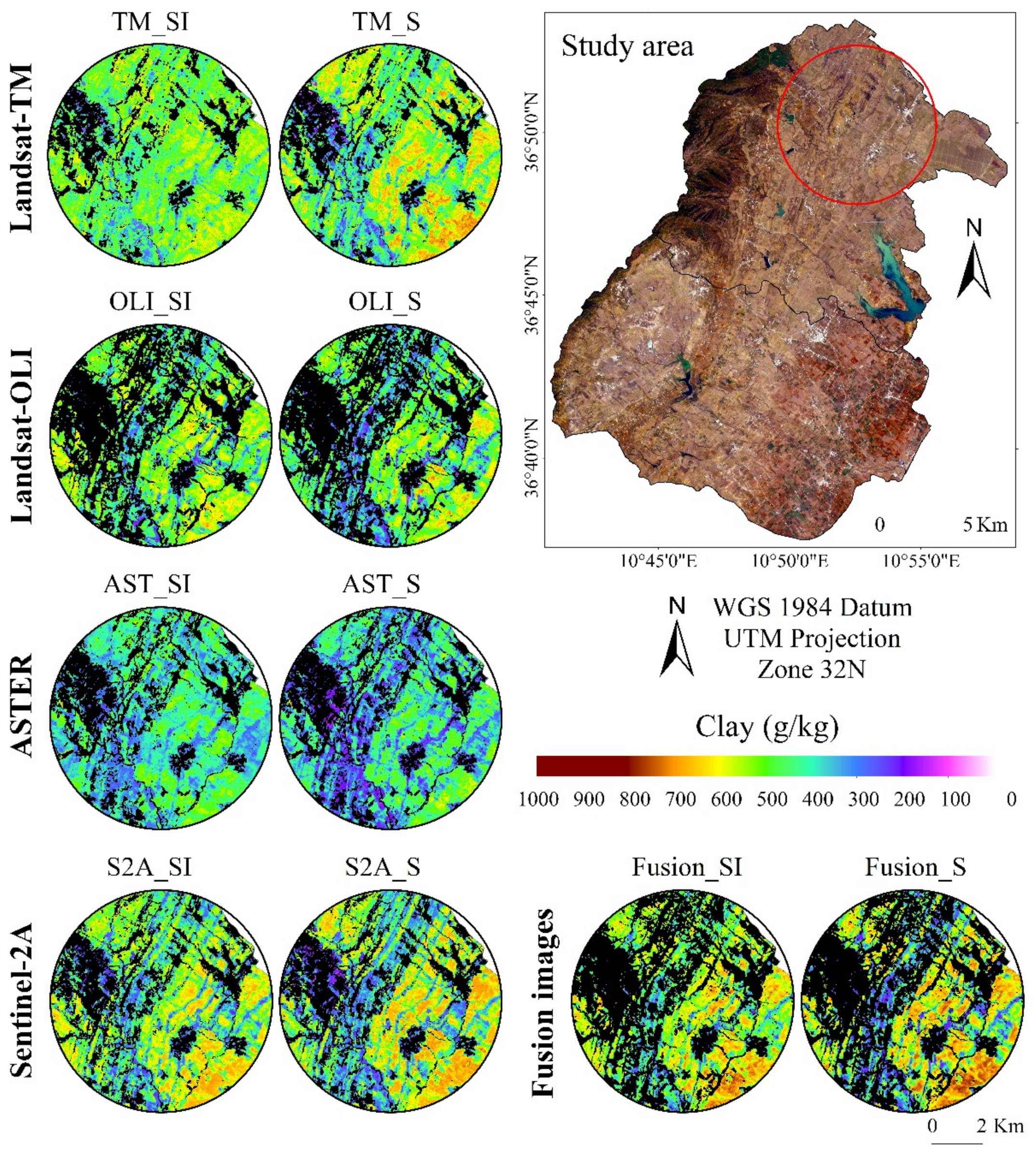
2.1. Study Area

The study was conducted over the Lebna and Chiba catchments within the Cap-Bon region in northeastern Tunisia (Figure 1a,b). The Lebna and Chiba catchments cover an area of 210 and 220 km2, respectively [28]. The catchments’ upstream components, mainly in the northwestern region, have mountainous relief, while the downstream components, corresponding to the southeastern region, have a flat area (Figure 1b). The Jebel Abderrahmane is the western limit of the upstream section of the Lebna and Chiba watersheds, covered by scrubland and forest, with a maximum altitude of 650 m. The study area is an agricultural region with intense plant production, including fruit culture, field crops (cereals, legumes), fodder crops, grazing pastures, condiments, and olive cultivation. The area is distinguished by a broad range of parent materials, notably limestone, marls, sand, sandstones, dunes, and detrital deposits developed during the Cenozoic era. This lithological complexity has resulted in the evolution of several soil types, including Regosols, Calcic Cambisols, Vertisols, Cambisols, Rendzina, Ferralitic, and Iso-humic soils [29].
Both catchments have a typical Mediterranean climate, with hot, dry summers and pleasant, chilly winters. Climate influence varies from a rainy regime at the top of the Jebel in the northwest, with more than 700 mm/year, to a semi-arid climate in the southeast, with less than 500 mm/year. The rainy season begins at the end of September and continues through February with moderate rain. The evaporative demand is roughly 1200 mm. In the summer, the highest temperature can reach 45 °C.

2.2. Soil Dataset and Sampling Collection

Soil samples were taken at a 0–5 cm depth during the soil studies conducted between October 2008 and November 2010. Five sub-samples were taken at random at every soil sample site inside a 10 × 10 m2 square plot. The central geographical position was registered using a Garmin GPS navigation system and georeferenced. The clay content (granulometric fraction inferior to 2 μm) was measured using the pipette method (method NF 31–107, particle size distribution by sedimentation) after drying, homogenizing, and sieving to 2 mm of all the samples [30].

2.3. Multispectral Satellite Data and Bare Soil Images

2.3.1. Multispectral Satellite Data

Multispectral satellite images acquired by Landsat-5 TM [31], Landsat-8 OLI [31], ASTER [32], and Sentinel-2A MSI [33] were used for the purpose of this study (Table 1). The Landsat-TM and OLI images were level-1 precision terrain (L1TP) products. The ASTER images were level-1 precision terrain, corrected and registered, at-sensor radiance (AST_L1T) products. The Sentinel-2A MSI image was a level-1C top-of-atmosphere (TOA) reflectance data product. One scene of the Landsat-TM, Landsat-OLI, and Sentinel-2A data and two scenes of the ASTER data were selected to cover the entire study area and were registered on 14 August 2008, 27 July 2013, 30 August 2015, and 03 July 2004, respectively, (Table 1). The multispectral satellite images were chosen during the summer season to avert the soil moisture caused by rain, cloud cover, and the impact of green vegetation. All images were radiometrically calibrated, atmospherically corrected, and converted to surface reflectance using the QUick Atmospheric Correction (QUAC) method [34]. The blue, green, red, and NIR1 bands of the Sentinel-2A image (i.e., bands 2, 3, 4, and 8A, respectively) were resampled to 20 m using the resample toolbox and the nearest neighbor technique [35] in ENVI software to guarantee that all Sentinel-2A spectral bands had an equal spatial resolution. The same treatment was carried out for the ASTER spectral bands with 15 and 30 m pixel sizes (band B1 to B3N and band B4 to B9), which were resampled to 30 m.

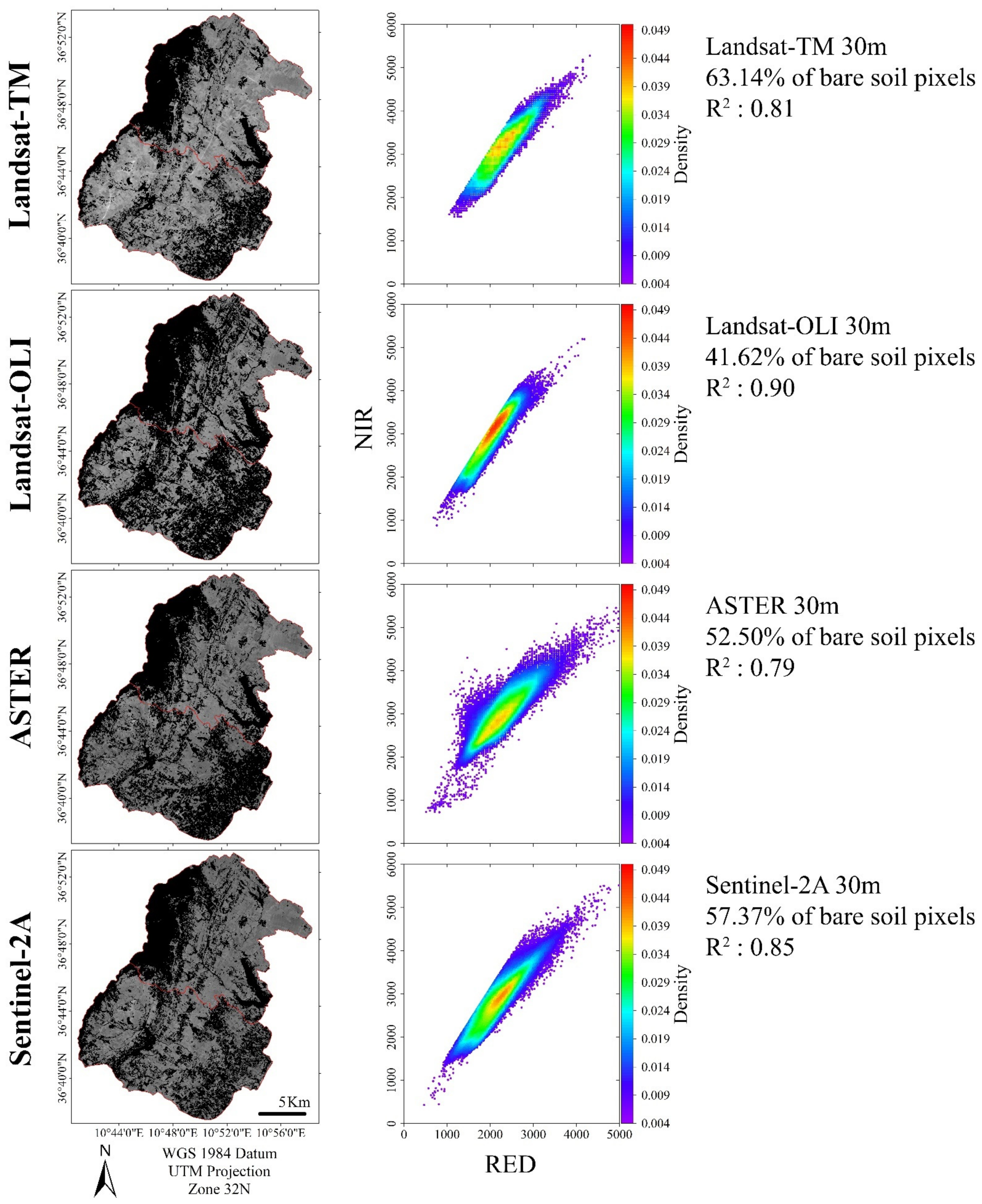
2.3.2. Bare Soil Images

The normalized difference vegetation index (NDVI) [36,37] was generated to mask the green vegetation in each image. Following a field visual inspection of different plots, a threshold value of NDVI equal to 0.22 was determined. Pixels with a reflectance value of less than 0.25 at 2100 nm, corresponding to bands 7 for the Landsat-TM and OLI, and bands 5 and 12 for the ASTER and Sentinel-2A, respectively, were designated dry vegetation coverage pixels and also masked. Pixels with a reflectance value of less than 0.28 at 1600 nm, corresponding to bands 5, 6, 4, and 11 of the Landsat-TM, OLI, ASTER, and Sentinel-2A, respectively, were considered as pixels covered by water and were also masked. The urban areas were also masked following a visual inspection. For further analysis, the green and dry vegetation, water, and urban areas were removed based on these diverse masks to maintain bare soil pixels in the satellite images, which we will refer to as the “bare soil images”.

2.4. Multi-Sensor Image Fusion

The Sentinel-2A MSI bare soil image has a spatial resolution of 20 m, and to group with the Landsat-5 TM, Landsat-8 OLI, and ASTER bare soil images, it was resampled to 30 m using the nearest neighbor method [35] in ENVI software. The Landsat-5 TM, Landsat-8 OLI, ASTER, and Sentinel-2A bare soil images at 30 m pixel sizes were named TM_S, OLI_S, AST_S, and S2A_S, respectively. A fifth image was obtained by fusing bare soil pixels onto only the common areas between these images (i.e., TM_S, OLI_S, AST_S, and S2A_S images) and was denoted as Fusion_SB. The resulting Fusion_SB image with 31 spectral bands at a 30 m spatial resolution was performed using the ENVI layer stacking tool.

2.5. Spectral Index Images

Spectral index images of the clay contents, named TM_SI, OLI_SI, and S2A_SI, were generated using the spectral index proposed by [19] from the TM_S, OLI_S, and S2A_S bare soil images, respectively, as follows:
ClayIndex CI =   SWIR 1 / SWIR 2
where SWIR1 corresponded to the spectral range from 1550 to 1750 nm, 1570 to 1650 nm, and 1565 to 1655 nm, for the TM_S, OLI_S, and S2A_S images, respectively (Table 1). SWIR2 corresponded to the spectral range from 2080 to 2350 nm, 2110 to 2290 nm, and 2100 to 2280 nm, for the TM_S, OLI_S, and S2A_S images, respectively (Table 1).
A spectral index image of the clay contents, named AST_SI, was generated from the AST_S bare soil image, using the spectral index proposed by [38] as follows:
ClayIndex CI _ AST =   SWIR 2 × SWIR 4 / SWIR 3
where SWIR2, SWIR3, and SWIR4, corresponded to the spectral ranges from 2145 to 2185 nm, 2185 to 2225 nm, and 2235 to 2285 nm, respectively, and corresponding to the AST-band B5, AST-band B6, and AST-band B7, respectively.

2.6. Multi-Sensor Satellite Data Fusion of Spectral Index Images

All satellite clay spectral index images (i.e., TM_SI, OLI_SI, AST_SI, and S2A_SI) were fused on the only common area to form a single image with 30 m of spatial resolution, which reunited the four clay spectral index images, named Fusion_SI. This data fusion integrated the clay spectral index images derived from several multispectral remote sensing datasets at different spatial, spectral, and temporal resolutions to collect more abundant information. The spectral index processing and data fusion were implemented using the ENVI software.

2.7. Statistical Analysis

2.7.1. Soil Line Analysis

The soil line analysis approach [39] was used to determine if the applied masks may successfully recover bare soil pixels from each multispectral image (i.e., TM_S, OLI_S, AST_S, and S2A_S images). The reflectance values of the NIR and Red bands corresponding to the TM-bands B4 and B3, OLI-bands B5 and B4, AST-bands B3 and B2, and S2A-bands B8 and B4 (Table 1), were plotted on an XY graph, and regression analyses were conducted between them. The better the coefficient of determination (R2) between the reflectance values of the NIR and Red bands, the nearer the scatter points were to the 1:1 line. Therefore, the applied masks were able to isolate the bare soil patches correctly.

2.7.2. Canonical Correlation Analysis

Canonical correlation analysis (CCA) [40,41] was carried out between the four multispectral images and only in the common bare soil pixels (i.e., on TM_S, OLI_S, AST_S, and S2A_S) to evaluate the spectral similarities between them. Each image’s spectral bands were reduced to discrete canonical variables using a multivariate linear transformation, equivalent to substituting a group of variables with uncorrelated components [41]. The higher the canonical correlations, the greater the spectral signatures were comparable amongst the multispectral images. This analysis was performed using SPSS software.

2.7.3. Pearson’s Correlation Analysis

Pearson’s correlation coefficient (r) was performed between the clay values and both the spectral band and spectral index values to evaluate the relevance of the derived remote sensing data for the clay content prediction. The p-value indicates whether the clay values were statistically significantly correlated with the spectral bands and spectral index in the Pearson’s correlation analysis.

2.7.4. Spatial Regression Models

The predictions of the soil clay content using TM, OLI, AST, S2A, and fusion images were performed following two approaches: (a) using the spectral index of each multispectral image (i.e., TM_SI, OLI_SI, AST_SI, S2A_SI, and Fusion_SI) and (b) the VNIR-SWIR spectral bands of each multispectral image (i.e., TM_S, OLI_S, AST_S, S2A_S, and Fusion_SB), as predictors, for a total of ten predictor images (Figure 2). The soil sample datasets for each image were split into training (75%) and validation (25%) using the Unscrambler software package [42]. The response variables (i.e., Yclay, clay content) were ordered in increasing rank. The lower clay content sample was first attributed to a validation set, followed by the next three samples in the training set. The process was then carried out by successively placing the next sample in the validation set and the subsequent three samples in the training set. This division guaranteed that the clay content in the training and validation sets was distributed similarly.
In this study, we relied on AutoML to select the best regression model and corresponding hyper-parameters on the given data. We chose to run the Auto-WEKA [43], which is an AutoML system based on the popular machine learning and data mining platform, WEKA software [44]. Auto-WEKA was the first AutoML system that considered the problem of simultaneously selecting a machine learning algorithm and optimizing its hyperparameters.
Among the popular machine learning algorithms, the Multi-Layer Perceptron (MLP) [45] network with a backpropagation (BP) algorithm has been widely used in practice for classification and regression problems. The MLP is a neural network that has a number of hidden layers of neurons. The connections between the neurons have a weight, which is obtained from a backpropagation algorithm. In the experiments, only one hidden layer was used in the MLP. The number of neurons in this layer, the learning rate, and momentum parameters were optimized through internal cross-validation in order to maximize the precision and accuracy of the results. The WEKA Multisearch package was used for this purpose.

2.7.5. Variable Selection Using MLP-BP Mean Decrease in Accuracy (MDA)

Feature selection was used to select the most pertinent and discriminative bands from the Fusion_SB image. Thus, it could identify and reduce as much irrelevant and redundant information as possible, thereby leading to the good predictive performance of the soil clay content. A mean decrease accuracy (MDA) [46] based on multilayer perceptron with the backpropagation learning algorithm (MLP-BP) evaluated the available band’s characteristics and ranked all bands based on the variable importance criterion for each band. MDA utilized the capability of the MLP-BP to evaluate the spectral bands of the Fusion_SB image during the training stage. After the MDA rankings, the spectral bands that had zero or negative contributions to the predicting clay content were removed from the Fusion_SB image. The remaining bands were then examined in descending order of MLP-BP models, with the smallest and most accurate model being kept. In more detail, if the introduction of a spectral band provided no increase in the model accuracy, then the said band was removed from the Fusion_SB image. At the final step of the procedure, we obtained a fusion image with the most discriminant features and this was denoted as Fusion_S.

2.7.6. Model Performances Assessment

The performance in the validation sets of the MLP-BP models was evaluated by the coefficient of determination of validation ( R val 2 ), the root mean square error of prediction (RMSEP), the mean absolute error of prediction (MAEP), the bias of prediction on validation sets, the ratio of the performance to the deviation on the validation set (RPD, [47]) and the ratio of performance to interquartile on the validation set (RPIQ, [48]). The predicted clay values and the produced maps were realized using the prediction tools of the WEKA software [44] and the ArcGis software package [49].

2.7.7. Spatial Structure Analysis

The spatial structure of the predicted clay contents was evaluated by examining their variogram characteristics, which quantified their spatial dependence. The semi-variance for the soil clay values to be displayed on a variogram was calculated using the formula [50]:
γ h = 1 2 N h i = 1 N h z x i z x i + h 2
where h is the lag distance, γ h is the semi-variance of the soil clay content at a lag distance h, N h is the total population of sample pairs at lag distance h, z is the value of the clay content, x is the position of point i on the landscape, and z x i + h is the clay value at the position x i + h . The variograms were calculated for the observed values dataset and maps estimated by spectral index (i.e., TM_SI, OLI_SI, AST_SI, and S2A_SI), spectral bands (i.e., TM_S, OLI_S, AST_S, and S2A_S), and image data fusion (i.e., Fusion_SI and Fusion_S) using Surfer-15 software (Golden Software, LLC).

3. Results

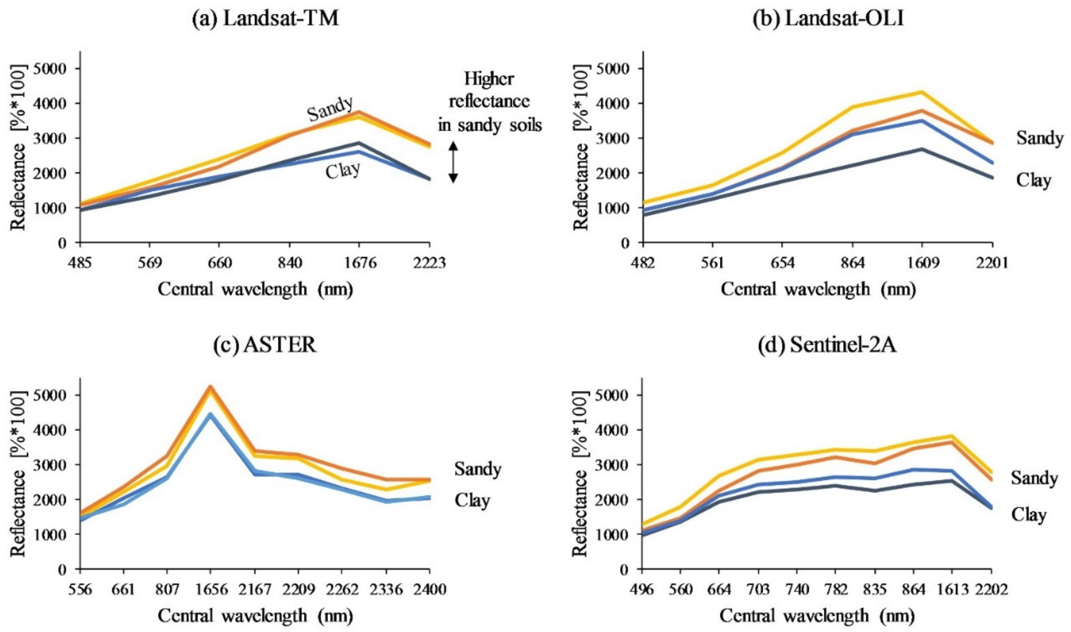
3.1. Bare Soil Images and Spectral Pattern Descriptions

The TM image had the highest bare soil pixels percentage (63.14%), followed by the S2A (57.37%), AST (52.50%), and OLI (41.62%) images (Figure 3). The bare soil’s surface variation was related to the different acquisition years of the multispectral scenes. According to the soil line analysis, the OLI image best described the bare soil patterns in the study region, with the highest coefficient of determination ( R 2 = 0.90). In contrast, the AST image had the lowest representation ( R 2 = 0.79) of all the examined images (Figure 3). The four multispectral remote sensing datasets had 34.6% of the common bare soil pixels. The canonical correlation analysis between these common bare soil pixels showed that the TM and OLI, as well as the OLI and S2A, had the highest coefficient (0.90) (Table 2). The percentage of bare soil pixels over both fusion images (i.e., Fusion_SI and Fusion_SB) was equal to 34.6%, which corresponds to the common bare soil area between all derived-multispectral images.
Based on the spectral characteristics of multispectral satellite images (i.e., TM, OLI, AST, and S2A images) (Figure 4), the reflectance values rose as the clay content dropped [8]. The TM and OLI spectra appeared very similar (Figure 4a,b). The reflectance values of the sandy soils were greater than those of the clay soils; however, the differences were noticeable in the NIR-SWIR wavebands regardless of the sensor (Figure 4).

3.2. Descriptive Statistics of Clay Soil Samples and Correlation with Bare Soil Images

The entire soil sample dataset contained 262 soil measurements. Due to the different number of bare soil pixels in each image, the dataset was reduced to 221, 174, 196, 218, and 149 soil data for the TM, OLI, AST, S2A, and fusion images, respectively (Table 3). The descriptive statistics results of the sample datasets used for each satellite image revealed a significant degree of similarity between the clay content values of the soil sample datasets. Based on the analysis of variance (ANOVA) results, no significant variations in the analyzed clay content values were observed at the 0.01 alpha level. The coefficient of variation (CV, reported in percent) was between 41 and 45% in all datasets. The TM soil samples had the highest CV, indicating that the TM soil sample set was the most varied in these datasets. In all datasets, the interquartile and standard deviation ranged from 283 to 302 g/kg and 179 to 182 g/kg, respectively. Finally, a soil sample with a clay content of 772 g/kg was reported in all datasets (Table 3).
The Pearson’s correlation coefficients between the spectral bands of the TM, OLI, AST, and S2A bare soil images and the measured clay values (Table 4) showed the significantly correlated bands of multispectral images with the measured clay values (p-value less than 0.05). All the spectral bands of the satellites’ multispectral images revealed a negative correlation with the soil clay content values. All datasets’ clay values demonstrated high correlation coefficients with the Red, RedEdge, NIR, and SWIR bands of the multispectral images (Table 4). The clay content was most correlated with the spectral bands TM-B7, OLI-B7, AST-B8, and S2A-B12, with r values equal to −0.72, −0.71, −0.67, and −0.72, respectively (Table 4). This most correlation is due to the clay minerals’ characteristic hydroxyl absorption around 2200 nm, caused by a mixture of vibrations related to the OH and OH-Al-OH bonds [15,51].
All clay value datasets were significantly correlated with the clay spectral index of each multispectral image, although the S2A_SI had the highest correlation (r = −0.71, Table 5).

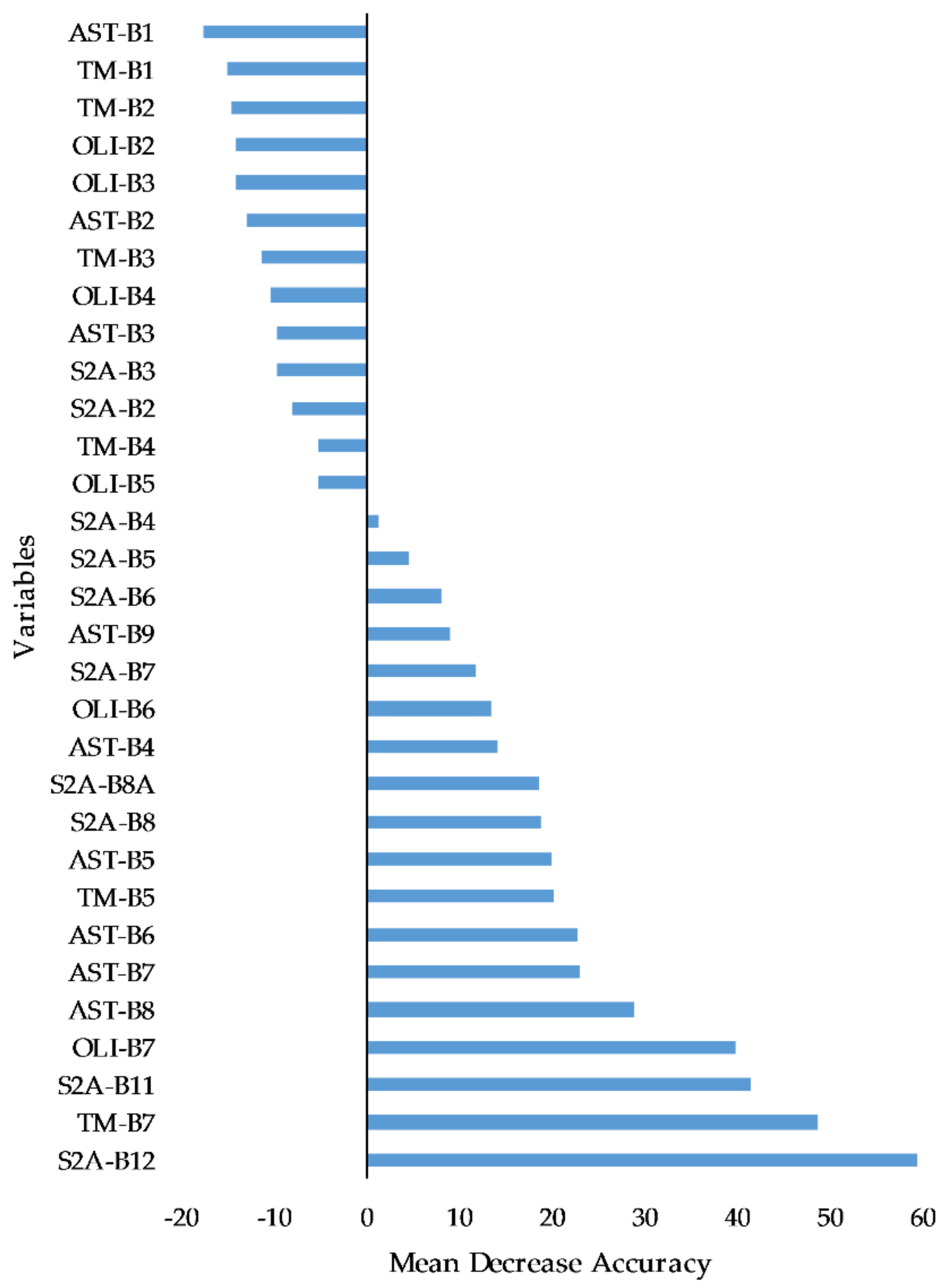
3.3. Selected Features from the Spectral Bands of the Fusion Image

The importance of each spectral band of the Fusion_SB image was derived from the MDA based on the MLP-BP algorithm and plotted on Figure 5 in order to investigate the feature rankings. The spectral bands S2A-band B12 (2100–2280 nm) and TM-band B7 (2080–2350 nm) were the most important for predicting the soil clay content. This spectral range had a central wavelength of around 2200 nm, which corresponds to an absorption characteristic caused by the combination of OH-Al bending and OH stretching modes [15]. Other variables that exerted important impacts were the S2A-band B11, followed by the OLI-band B7 and AST-band B8 (Figure 5). The AST-band B7, AST-band B6, TM-band B5, AST-band B5, S2A-band B8, S2A-band B8A, AST-band B4, and OLI-band B6 were identified as the factors group with a moderate importance to predict soil clay content. The other variables (i.e., S2A-band B7, AST-band B9, S2A-band B6, S2A-band B5, and S2A-band B4) emerged as having weak impacts. Although these variables might not be particularly predictive by themselves alone, some can increase the model accuracy through their interactions with other variables [52]. Additionally, thirteen bands had no impact on the prediction performance (Figure 5). Finally, from the Fusion_SB image, the variable selection using the MDA based on MLP-BP selected a feature subset of eight attributes for the clay prediction. This feature subset included the spectral bands S2A-band B12, TM-band B7, OLI-band B7, TM-band B5, S2A-band B8, OLI-band B6, S2A-band B7, and AST-band B9, which were selected to generate the Fusion_S image.

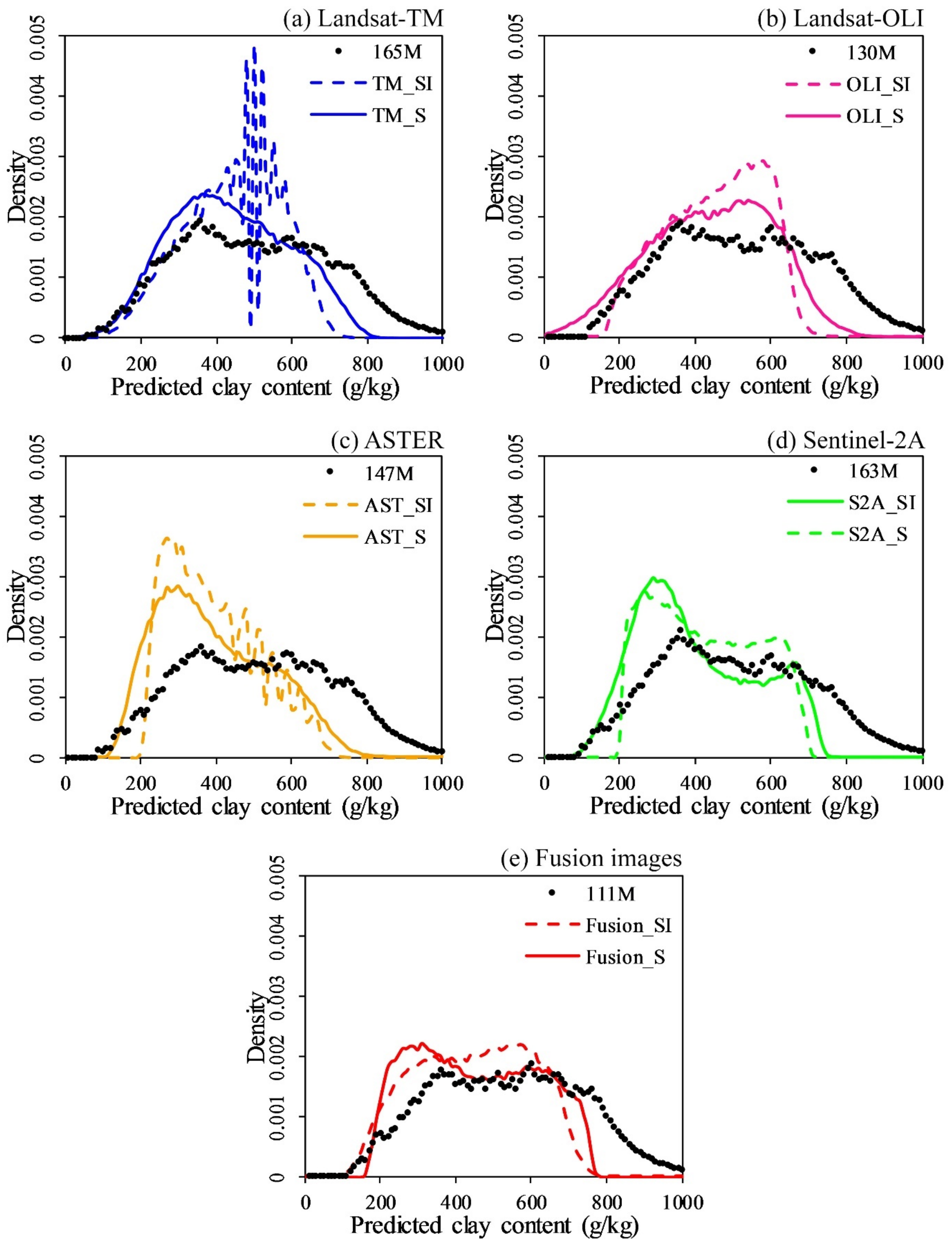
3.4. Spectral Index vs. Spectral Bands Prediction Performances

Based on the Auto-WEKA results, the MLP-BP was selected as the best regression model for the datasets. The MLP-BP models generated from spectral index images (i.e., TM_SI, OLI_SI, AST_SI, and S2_SI) performed poorly regardless of the sensor (0.43 ≤ R val 2 ≤ 0.51, and 126.42 ≤ RMSEP ≤ 140.24 g/kg, Table 6); however, the MLP-BP model built from the spectral index image fusion (Fusion_SI) provided good performance ( R val 2 = 0.61 and RMSEP = 114.18 g/kg, Table 6), outperforming the MLP-BP models built from individual spectral index images (Table 6).
The MLP-BP models created from the multispectral images (TM_S, OLI_S, AST_S, and S2A_S) showed accurate results (0.60 ≤ R val 2 ≤ 0.71, and 96.45 ≤ RMSEP ≤ 115.64 g/kg, Table 6), whereas the clay prediction model built using the S2A_S spectra provided the higher performance, taking advantage of the sentinel-2 MSI sensor’s ten spectral bands. The clay prediction model created using the AST_S spectra performed worse, although the ASTER sensor had nine spectral bands. The MLP-BP model built from the fusion image (Fusion_S) performed excellently ( R val 2 = 0.78, and RMSEP = 87.84 g/kg, Table 6), outperforming the MLP-BP models built from individual multispectral images (Table 6).

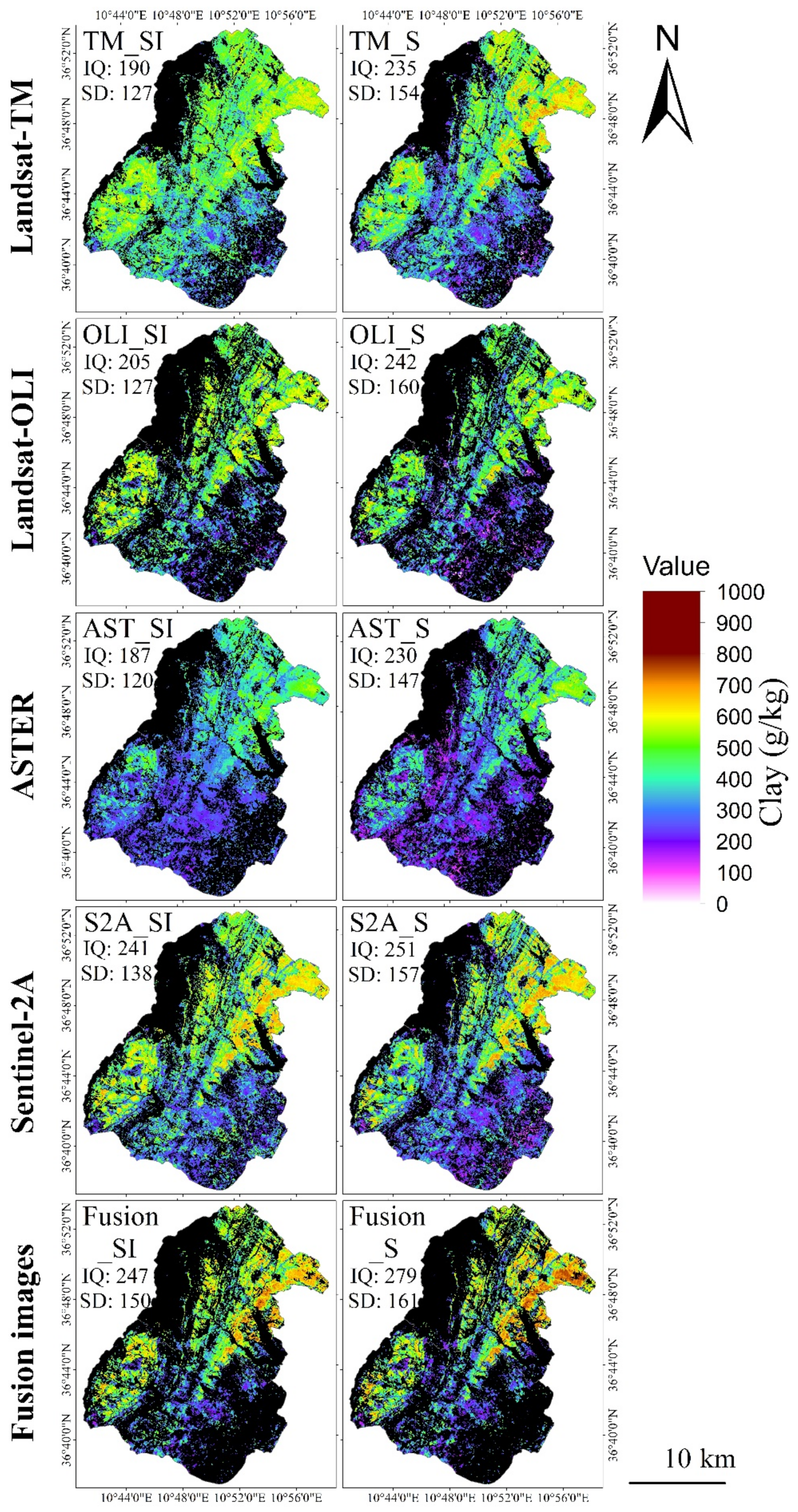
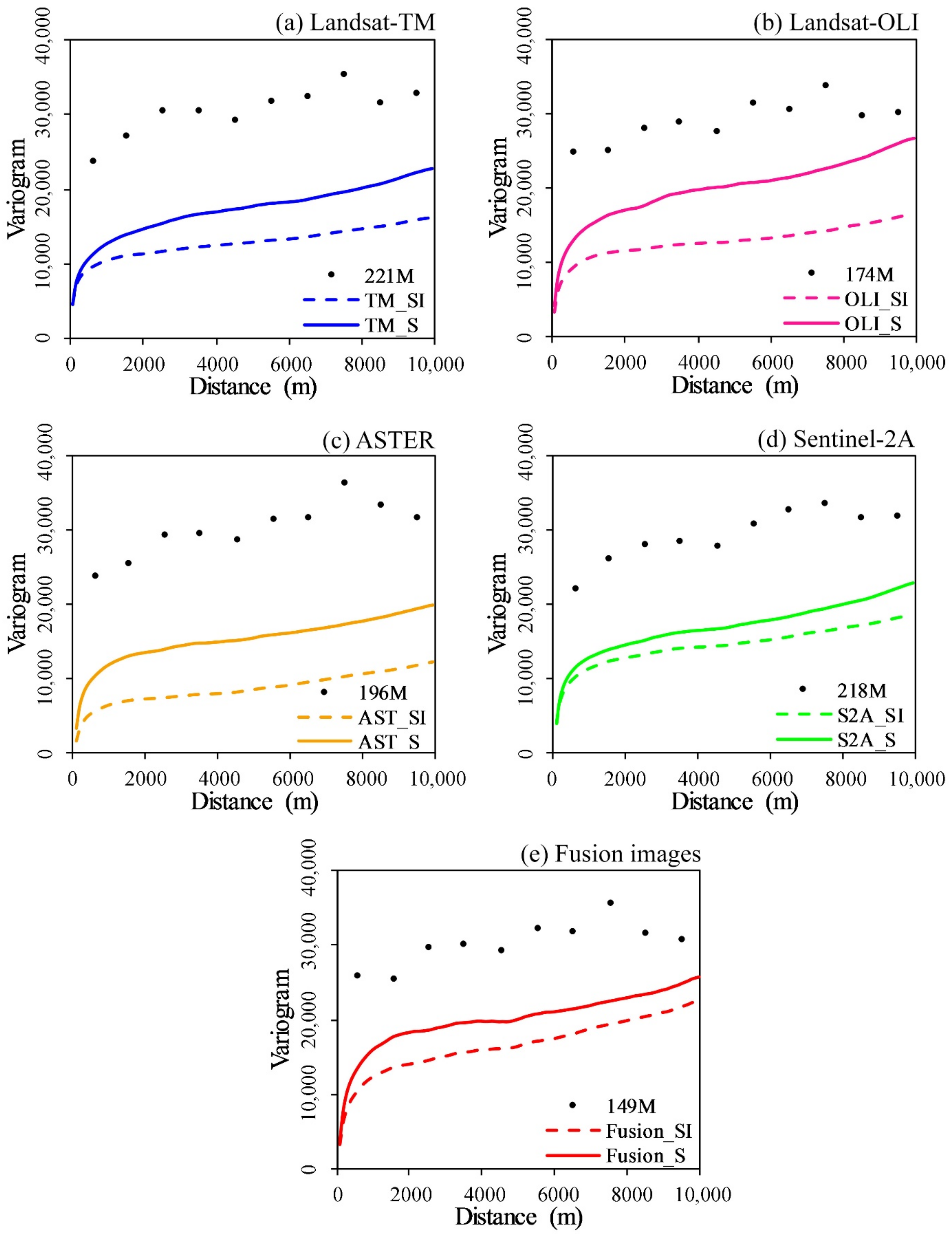
3.5. Predicted Soil Maps and Spatial Structure Analysis

The MLP-BP models were applied to their corresponding bare soil images to provide the predicted clay content maps (Figure 6). The predicted clay content maps derived from the spectral index approach showed a globally similar distribution of clay spatial patterns regardless of the percentage of bare soil areas, as was the case for the maps derived from the VNIR-SWIR spectral bands approach. On these predicted clay maps, the south-eastern part of the studied area presented low concentrations of soil clay, whereas the north-eastern part of the area presented high concentrations, regardless of the map (Figure 6). Moreover, the clay content map predicted using the Fusion_S showed clay content values slightly higher than the other maps, regardless of the maps region.
For each satellite sensor, both the spectral index and VNIR-SWIR spectral bands images were able to represent the variability of the soil clay content; however, with the spectral images, the interquartile and standard deviation values were higher than those obtained with the spectral index images. Both the Fusion_SI and Fusion_S clay content maps, which had the best performance (Table 6), showed high interquartile and standard deviation values in contrast to the other predicted maps. Depending on the images used to create the predicted clay maps, the IQ varied from 187 g/kg (obtained from the AST_SI image) to 279 g/kg (obtained from the Fusion_S image). Thus, the standard deviation varied from 120 g/kg (obtained from the AST_SI image) to 161 g/kg (obtained from the Fusion_S image) (Figure 6).
Figure 7 shows a zoom over a small area of the predicted clay maps, characterized by strong variations in the soil patterns on a small scale, with a close succession of clay-rich areas (brown color) and clay-poor areas (sky blue color) oriented northwest/southeast, corresponding to marl and sandstone outcrops, respectively. Following the VNIR-SWIR spectral bands approach, the predicted clay maps exhibited more clearly short-range variations in soil patterns, with a close succession of clay-rich areas and clay-poor areas, than the maps following the spectral index approach (Figure 7). Between the clay maps based on the fusion of the spectral index and VNIR-SWIR spectral bands images, the Fusion_S showed slightly higher clay values than the Fusion_SI values. It should be noted that the changes in the bare soil spatial coverage are small among the Landsat-5 TM, Landsat-8 OLI, ASTER, and Sentinel-2A images (Figure 7).
Histograms analysis of the predicted maps over the Lebna and Chiba catchments showed a normal distribution of clay content, with the exception of the histogram of predicted values from the TM_SI around 500 g/kg, which represents an extremely weak density (Figure 8). The histograms of predicted values from the TM, AST, and S2A images showed a histogram peak of around 300 g/kg, while the histograms of predicted values from the OLI image showed a histogram peak of around 500 g/kg (Figure 8). This may be due to the training database’s clay values, which were slightly higher than the other databases (see Table 3 and Figure 8). Moreover, the distribution of clay contents predicted using the spectral index images (TM_SI, OLI_SI, AST_SI, and S2A_SI) shifted to slightly higher values compared to those obtained from the VNIR-SWIR spectral bands images. This means that the pedological variability of the study area is more represented in the predicted clay content maps obtained using the VNIR-SWIR spectral bands images (TM_S, OLI_S, AST_S, and S2A_S) than in the spectral index images (TM_SI, OLI_SI, AST_SI, and S2A_SI). Thus, the maps predicted using the fusion images exhibited a wider distribution of clay content values than the other images (Figure 8).
Finally, the variograms of the measured clay content values (dots in Figure 9) had higher variance than the predicted values, regardless of the sample datasets used for each satellite image. Thus, the spatial structures of the estimated clay contents obtained by the VNIR-SWIR spectral bands images exhibited very high sills compared to the spectral index images (Figure 9). By contrast, the variance obtained by the spectral index image fusion exhibited a very high sill and strong variations compared to those obtained by a single sensor spectral index image. Finally, the variogram obtained by the VNIR-SWIR spectral bands image fusion was higher.

4. Discussion

4.1. Clay Predictions Depending on the Multispectral Sensor

The models based on multispectral images (i.e., TM_S, OLI_S, AST_S, and S2A_S) provided acceptable accuracies with R val 2 values between 0.60 and 0.71, RMSEP values between 96.45 and 115.64 g/kg, MAEP values between 73.29 and 91.86 g/kg, RPD values between 1.60 and 1.90, and RPIQ values between 2.59 and 3.01 (Table 6). This performance variance could be explained by differences in satellite remote sensing datasets’ acquisition dates (i.e., date ranges), as previously shown by [53]. Moreover, though the bands of each sensor cover similar spectral domains, they were not exactly the same (Table 1). Additionally, different acquisition conditions and view angles between the sensors can result in differences between the recorded datasets [54]. The model performance obtained from the S2A_S image was superior to that obtained by [6], who also used the ten bands of the Sentinel-2A (S2A) and a PLSR model. Similar results were obtained by [8] using Sentinel-2 MSI and Landsat-8 OLI images for clay content prediction, with R2 values of 0.68 and 0.62, respectively. Moreover, [29] also found similar performance using the MLR model and nine bands of the ASTER image, while [55] obtained a high prediction accuracy of soil clay content using a mean spectral reflectance from bare soil pixels along a Landsat-TM time series.

4.2. Clay Predictions Obtained from Spectral Indexes vs. Entire Spectra

Whatever the sensor, the models built using the entire VNIR-SWIR spectra outperformed the models built using spectral indexes (Table 6). The models built from the four spectral index images (i.e., TM_SI, OLI_SI, AST_SI, and S2A_SI) performed poorly (0.43 ≤ R val 2 ≤ 0.51, 126.42 ≤ RMSEP ≤ 140.24 g/kg, 99.65 ≤ MAEP ≤ 112.29 g/kg, 1.34 ≤ RPD ≤ 1.45, and 2.14 ≤ RPIQ ≤ 2.30, respectively; Table 6), and this could be explained by the lack of spectral information. These prediction accuracy results were in agreement with those obtained by [23], who used a Simple Ratio Clay Index (SRCI) and a Normalized Difference Clay Index (NDCI) based on Landsat-OLI imagery for clay content mapping in Indonesia. Accuracy assessment of the regression models based on independent validation showed that both clay indexes provided low performances, with R 2 values of 0.42 and 0.40, respectively [23]; however, [24] used Simple Linear Regression (SLR) to establish the relationships between many NDCI-Landsat TM and clay content over the Kairouan plain in Tunisia and obtained results with R 2 values that varied between 0.48 and 0.73.

4.3. Added-Value of Fusion Images

The best-performer models were obtained using multi-sensor image fusion incorporating spectral bands or spectral index images (Table 6). Effectively, the model with the best performance for the spectral bands approach was founded on the Fusion_S image, with an R val 2 of 0.78, an RMSEP of 87.84 g/kg, an MAEP of 69.99 g/kg, an RPD of 2.12, and an RPIQ of 3.25 (Table 6). Similarly, for the spectral index approach, the model based on the Fusion_SI image was superior to those found on the TM_SI, OLI_SI, AST_SI, and S2A_SI (Table 6).
On the other hand, based on the same soil sample set (i.e., 149 samples), the models using multispectral images (i.e., TM_S, OLI_S, AST_S, and S2A_S) provided acceptable results with R val 2 values between 0.48 and 0.69, RMSEP values between 99.94 and 132.31 g/kg, MAEP values between 82.89 and 109.93 g/kg, RPD values between 1.40 and 1.86, and RPIQ values between 2.16 and 2.86 (results not shown). These performances, however, always remained lower than those obtained using the Fusion_S (Table 6). The models based on the four spectral index datasets (i.e., TM_SI, OLI_SI, AST_SI, and S2A_SI) and the same soil samples (i.e., 149 samples) performed poorly in estimating the clay content with R val 2 values between 0.21 and 0.53, RMSEP values between 125.03 and 162.89 g/kg, MAEP values between 99.36 and 130.59 g/kg, RPD values between 1.14 and 1.49, and RPIQ values between 1.75 and 2.28 (results not shown), and these performances always remained lower than those obtained using Fusion_SI (Table 6).
The results of this paper suggest that the models based on satellite multi-sensor data fusion were the most precise for prediction and mapping of soil clay content. Moreover, the improved accuracy of the results obtained using fusion images might be attributed to complementary spectral, spatial, and temporal information derived from the fusion of various satellite sensor datasets. For example, [4] demonstrated the potential of using fusion indices derived from multitemporal Landsat 8 imagery to predict static soil properties such as OC, sand, and CCE. Meanwhile [26] investigated multisource data fusion for topsoil clay mappings, such as proximally measured gamma (γ) ray spectrometry, apparent electrical conductivity (ECa), four terrain attributes, and the digital numbers (DNs) of an aerial photo. The results improved when the gamma-ray spectrometry data was integrated with the digital numbers (DNs) of the aerial photos [26]. Ref. [27] established an empirical surface soil moisture (SSM) model via the fusion of soil moisture networks, remote sensing data, and high-resolution land surface parameters. The results indicated that the data fusion-based model could retrieve the SSM temporal dynamics [27].

4.4. Future Research

In this study, the best results were obtained via the fusion of four multispectral satellite images with feature selection using an MDA based on MLP-BP, which allowed the selecting of the most significant, pertinent, and discriminative spectral bands to predict clay content (i.e., eight bands), instead of just using six bands for the TM or OLI, for example. Thus, the modelling process produced an increase of about 10% in the prediction accuracy compared to that obtained from single-sensor images. Nonetheless, only the variable selection using the MDA based on the MLP-BP algorithm was used to select the key features impacting clay prediction; however, future research could consider using additional feature selection methods, including feature subset evaluation and feature ranking methods belonging to three groups: filter, wrapper, and embedded techniques. Finally, the incorporation of additional data sources to generate the fusion image, such as thermal infrared bands, synthetic aperture radar (SAR) and light detection and ranging (LiDAR) data, can improve the accuracy of the results for soil property prediction.

5. Conclusions

Spectral bands images restricted to bare soil pixels, derived from Landsat-TM, Landsat-OLI, ASTER, and the Sentinel-2A satellites, were more suitable for obtaining the soil clay map than those derived from the spectral index images of the same satellites. Moreover, the satellite’s multi-sensor data fusion, which included multispectral bands or spectral index images, was revealed to be a promising tool for mapping soil attributes. Multi-sensor images generated by the fusion of multispectral satellite data can provide a voluminous amount of bare soil information for DSM. To reinforce these conclusions and the guidelines, this study could be enlarged to (i) evaluate additional feature selection algorithms and methods, (ii) integrate additional data sources into the fusion image, (iii) assess the influence of the spatial resolution of the fusion image on soil property prediction, and (iv) include additional soil properties and additional pedological settings.

Author Contributions

Conceptualization, and methodology, A.G. and C.G.; remote sensing data pretreatments, software, and algorithms, A.G.; results analysis, all authors; field expertise, all authors; writing, all authors. The manuscript was improved by the contributions of all of the co-authors. All authors have read and agreed to the published version of the manuscript.

Funding

This research received no external funding.

Acknowledgments

The authors are grateful to Yves Blanca (IRD-UMR LISAH Montpellier), and Zakia Jenhaoui (IRD UMR LISAH Tunis) for conducting and supporting field soil sampling in 2009 and 2010 over the Lebna catchment, and to Hedi Hamrouni (DG/ACTA Sol, Tunis) and to everybody that directly or indirectly assisted in publishing this study. We want to thank the remote sensing editorial office, and three anonymous reviewers for their valuable and constructive comments.

Conflicts of Interest

The authors declare no conflict of interest.

References

  1. Lagacherie, P.; McBratney, A. Chapter 1. Spatial soil information systems and spatial soil inference systems: Perspectives for Digital Soil Mapping. In Digital Soil Mapping, an Introductory Perspective. Developments in Soil Science; Lagacherie, P., McBratney, A.B., Voltz, M., Eds.; Elsevier: Amsterdam, The Netherlands, 2007; Volume 31, pp. 3–24. [Google Scholar]
  2. Grunwald, S.; Thompson, J.A.; Boettinger, J.L. Digital Soil Mapping and Modeling at Continental Scales: Finding Solutions for Global Issues. Soil Sci. Soc. Am. J. 2011, 75, 1201–1213. [Google Scholar] [CrossRef]
  3. Mulder, V.; de Bruin, S.; Schaepman, M.; Mayr, T. The use of remote sensing in soil and terrain mapping—A review. Geoderma 2011, 162, 1–19. [Google Scholar] [CrossRef]
  4. Fathololoumi, S.; Vaezi, A.R.; Alavipanah, S.K.; Ghorbani, A.; Saurette, D.; Biswas, A. Improved digital soil mapping with multitemporal remotely sensed satellite data fusion: A case study in Iran. Sci. Total Environ. 2020, 721, 137703. [Google Scholar] [CrossRef] [PubMed]
  5. Gomez, C.; Dharumarajan, S.; Féret, J.-B.; Lagacherie, P.; Ruiz, L.; Sekhar, M. Use of Sentinel-2 Time-Series Images for Classification and Uncertainty Analysis of Inherent Biophysical Property: Case of Soil Texture Mapping. Remote Sens. 2019, 11, 565. [Google Scholar] [CrossRef] [Green Version]
  6. Vaudour, E.; Gomez, C.; Fouad, Y.; Lagacherie, P. Sentinel-2 image capacities to predict common topsoil properties of temperate and Mediterranean agroecosystems. Remote Sens. Environ. 2019, 223, 21–33. [Google Scholar] [CrossRef]
  7. Loiseau, T.; Chen, S.; Mulder, V.L.; Dobarco, M.R.; Richer-De-Forges, A.C.; Lehmann, S.; Bourennane, H.; Saby, N.P.A.; Martin, M.P.; Vaudour, E.; et al. Satellite data integration for soil clay content modelling at a national scale. Int. J. Appl. Earth Obs. Geoinf. 2019, 82, 101905. [Google Scholar] [CrossRef]
  8. Bellinaso, H.; Silvero, N.E.; Ruiz, L.F.C.; Amorim, M.T.A.; Rosin, N.A.; Mendes, W.D.S.; de Sousa, G.P.B.; Sepulveda, L.M.A.; de Queiroz, L.G.; Nanni, M.R.; et al. Clay content prediction using spectra data collected from the ground to space platforms in a smallholder tropical area. Geoderma 2021, 399, 115116. [Google Scholar] [CrossRef]
  9. Datt, B.; McVicar, T.; Van Niel, T.; Jupp, D.; Pearlman, J. Preprocessing eo-1 hyperion hyperspectral data to support the application of agricultural indexes. IEEE Trans. Geosci. Remote Sens. 2003, 41, 1246–1259. [Google Scholar] [CrossRef] [Green Version]
  10. Levin, N.; Kidron, G.J.; Ben-Dor, E. Surface properties of stabilizing coastal dunes: Combining spectral and field analyses. Sedimentology 2007, 54, 771–788. [Google Scholar] [CrossRef]
  11. Gomez, C.; Lagacherie, P.; Coulouma, G. Continuum removal versus PLSR method for clay and calcium carbonate content estimation from laboratory and airborne hyperspectral measurements. Geoderma 2008, 148, 141–148. [Google Scholar] [CrossRef]
  12. Lagacherie, P.; Baret, F.; Feret, J.-B.; Netto, J.M.; Robbez-Masson, J.M. Estimation of soil clay and calcium carbonate using laboratory, field and airborne hyperspectral measurements. Remote Sens. Environ. 2008, 112, 825–835. [Google Scholar] [CrossRef]
  13. Gomez, C.; Lagacherie, P.; Coulouma, G. Regional predictions of eight common soil properties and their spatial structures from hyperspectral Vis–NIR data. Geoderma 2012, 189–190, 176–185. [Google Scholar] [CrossRef]
  14. Gomez, C.; Gholizadeh, A.; Borůvka, L.; Lagacherie, P. Using legacy data for correction of soil surface clay content predicted from VNIR/SWIR hyperspectral airborne images. Geoderma 2016, 276, 84–92. [Google Scholar] [CrossRef]
  15. Chabrillat, S.; Goetz, A.F.; Krosley, L.; Olsen, H.W. Use of hyperspectral images in the identification and mapping of expansive clay soils and the role of spatial resolution. Remote Sens. Environ. 2002, 82, 431–445. [Google Scholar] [CrossRef]
  16. Gaffey, S.J. Spectral reflectance of-carbonate minerals in the visible and near infrared (0.35–2.55 microns): Calcite, aragonite, and dolomite. Am. Mineral. 1986, 71, 151–162. [Google Scholar]
  17. Viscarra Rossel, R.A.; Behrens, T.; Ben-Dor, E.; Brown, D.J.; Demattê, J.A.M.; Shepherd, K.D.; Shi, Z.; Stenberg, B.; Stevens, A.; Adamchuk, V.; et al. A global spectral library to characterize the world’s soil. Earth Sci. Rev. 2016, 155, 198–230. [Google Scholar] [CrossRef] [Green Version]
  18. Segal, D. Theoretical Basis for Differentiation of Ferric-Iron Bearing Minerals, Using Landsat MSS Data. In Proceedings of the 2nd Thematic Conference on Remote Sensing for Exploratory Geology, Symposium for Remote Sensing of Environment, Fort Worth, TX, USA, 6–10 December 1982; pp. 949–951. [Google Scholar]
  19. Drury, S.A. Image interpretation in geology. Geocarto Int. 1987, 2, 48. [Google Scholar] [CrossRef]
  20. Haubrock, S.-N.; Chabrillat, S.; Lemmnitz, C.; Kaufmann, H. Surface soil moisture quantification models from reflectance data under field conditions. Int. J. Remote Sens. 2008, 29, 3–29. [Google Scholar] [CrossRef]
  21. Weng, Y.-L.; Gong, P.; Zhu, Z.-L. A Spectral Index for Estimating Soil Salinity in the Yellow River Delta Region of China Using EO-1 Hyperion Data. Pedosphere 2010, 20, 378–388. [Google Scholar] [CrossRef]
  22. Mathieu, R.; Pouget, M.; Cervelle, B.; Escadafal, R. Relationships between Satellite-Based Radiometric Indices Simulated Using Laboratory Reflectance Data and Typic Soil Color of an Arid Environment. Remote Sens. Environ. 1998, 66, 17–28. [Google Scholar] [CrossRef]
  23. Danoedoro, P.; Zukhrufiyati, A. Integrating Spectral Indices and Geostatistics Based on Landsat-8 Imagery for Surface Clay Content Mapping in Gunung Kidul Area, Yogyakarta, Indonesia. In Proceedings of the 36th Asian Conference on Remote Sensing 2015 Fostering Resilient Growth, Quezon City, Metro Manila Philippines, 24–28 October 2015; Volume 1. Available online: https://www.researchgate.net/publication/302580476 (accessed on 12 January 2019).
  24. Shabou, M.; Mougenot, B.; Chabaane, Z.L.; Walter, C.; Boulet, G.; Aissa, B.N.; Zribi, M. Soil clay content mapping using a time series of landsat TM data in semi-arid lands. Remote Sens. 2015, 7, 6059–6078. [Google Scholar] [CrossRef] [Green Version]
  25. Zhang, J. Multi-source remote sensing data fusion: Status and trends. Int. J. Image Data Fusion 2010, 1, 5–24. [Google Scholar] [CrossRef] [Green Version]
  26. Piikki, K.; Söderström, M.; Stenberg, B. Sensor data fusion for topsoil clay mapping. Geoderma 2013, 199, 106–116. [Google Scholar] [CrossRef]
  27. Huang, J.; Desai, A.R.; Zhu, J.; Hartemink, A.E.; Stoy, P.C.; Loheide, S.P.I.; Bogena, H.R.; Zhang, Y.; Zhang, Z.; Arriaga, F. Retrieving Heterogeneous Surface Soil Moisture at 100 m Across the Globe via Fusion of Remote Sensing and Land Surface Parameters. Front. Water 2020, 2, 38. [Google Scholar] [CrossRef]
  28. Gasmi, A.; Masse, A.; Ducrot, D.; Zouari, H. Télédétection et photogrammétrie pour l’étude de la dynamique de l’occupation du sol dans le bassin versant de l’oued Chiba (Cap-Bon, Tunisie). Rev. Française Photogrammétrie Télédétection 2017, 215, 43–51. [Google Scholar] [CrossRef]
  29. Gasmi, A.; Gomez, C.; Lagacherie, P.; Zouari, H. Surface soil clay content mapping at large scales using multispectral (VNIR–SWIR) ASTER data. Int. J. Remote Sens. 2019, 40, 1506–1533. [Google Scholar] [CrossRef]
  30. Baize, D.; Jabiol, B. Guide Pour la Description des Sols; INRA Edition: Paris, France, 1995. [Google Scholar]
  31. NASA-Goddard Space Flight Center (GSFC). Available online: https://landsat.gsfc.nasa.gov (accessed on 29 September 2020).
  32. Gasmi, A.; Gomez, C.; Zouari, H.; Masse, A.; Ducrot, D. PCA and SVM as geo-computational methods for geological mapping in the southern of Tunisia, using ASTER remote sensing data set. Arab. J. Geosci. 2016, 9, 753. [Google Scholar] [CrossRef]
  33. ESA—European Space Agency. Available online: https://sentinel.esa.int/web/sentinel/technical-guides/sentinel-2-msi/msi-instrument (accessed on 11 December 2020).
  34. Bernstein, L.; Adler-Golden, S.; Sundberg, R.; Levine, R.; Perkins, T.; Berk, A.; Ratkowski, A.; Felde, G.; Hoke, M. A new method for atmospheric correction and aerosol optical property retrieval for VIS-SWIR multi- and hyperspectral imaging sensors: QUAC (QUick atmospheric correction). In Proceedings of the 2005 IEEE International Geoscience and Remote Sensing Symposium, 2005. IGARSS ‘05, Seoul, Korea, 29–29 July 2005. [Google Scholar]
  35. Dodgson, N.A. Image Resampling. University of Cambridge Computer Laboratory; University of Cambridge, Computer Laboratory: Cambridge, UK, 1992. [Google Scholar]
  36. Jordan, C.F. Derivation of Leaf-Area Index from Quality of Light on the Forest Floor. Ecology 1969, 50, 663–666. [Google Scholar] [CrossRef]
  37. Rouse, J.W.; Haas, R.H.; Schell, J.A.; Deering, D.W. Monitoring vegetation systems in the great plains with ERTS. In Proceedings of the Third Earth Resources Technology Satellite-1 Symposium, Washington, DC, USA, 3 September 2013; NASA SP-351. NASA: Greenbelt, MD, USA, 1974; Volume 1, pp. 309–317. [Google Scholar]
  38. Sadek, M.F.; Ali-Bik, M.W.; Hassan, S.M. Late Neoproterozoic basement rocks of Kadabora-Suwayqat area, Central Eastern Desert, Egypt: Geochemical and remote sensing characterization. Arab. J. Geosci. 2015, 8, 10459–10479. [Google Scholar] [CrossRef]
  39. Baret, F.; Jacquemoud, S.; Hanocq, J. About the soil line concept in remote sensing. Adv. Space Res. 1993, 13, 281–284. [Google Scholar] [CrossRef]
  40. Jordan, C. Essai sur la géométrie à n dimensions. Bull. Société Mathématique Fr. 1875, 3, 103–174. [Google Scholar] [CrossRef]
  41. Hotelling, H. Relations between Two Sets of Variates. Biometrika 1936, 28, 321. [Google Scholar] [CrossRef]
  42. CAMO. The Unscrambler X Software; CAMO: Oslo, Norway, 2018; Available online: www.camo.com (accessed on 28 October 2020).
  43. Kotthoff, L.; Thornton, C.; Hoos, H.H.; Hutter, F.; Leyton-Brown, K. Auto-WEKA: Automatic Model Selection and Hyperparameter Optimization in WEKA. In Automated Machine Learning; Frank, H., Ed.; Springer: Berlin/Heidelberg, Germany, 2019; pp. 81–95. [Google Scholar]
  44. Holmes, G.; Donkin, A.; Witten, I. WEKA: A machine learning workbench. In Proceedings of ANZIIS ‘94—Australian New Zealnd Intelligent Information Systems Conference, Brisbane, Australia, 29 November–2 December 1994; pp. 357–361. [Google Scholar] [CrossRef] [Green Version]
  45. Bishop, C.M. Neural Networks for Pattern Recognition; Oxford University Press: Oxford, UK, 1995. [Google Scholar]
  46. Breiman, L. Random forests. Mach. Learn. 2001, 45, 5–32. [Google Scholar] [CrossRef] [Green Version]
  47. Chang, C.-W.; Laird, D.A.; Mausbach, M.J.; Hurburgh, C.R. Near-Infrared Reflectance Spectroscopy-Principal Components Regression Analyses of Soil Properties. Soil Sci. Soc. Am. J. 2001, 65, 480–490. [Google Scholar] [CrossRef] [Green Version]
  48. Bellon-Maurel, V.; Fernandez-Ahumada, E.; Palagos, B.; Roger, J.-M.; McBratney, A. Critical review of chemometric indicators commonly used for assessing the quality of the prediction of soil attributes by NIR spectroscopy. TrAC Trends Anal. Chem. 2010, 29, 1073–1081. [Google Scholar] [CrossRef]
  49. ESRI. ArcGIS Desktop: Release 10.8. Environmental Systems Research Institute Inc., Redlands. 2018. Available online: https://www.esri.com (accessed on 2 November 2018).
  50. Webster, R.; Oliver, M.A. Statistical Methods in Soil and Land Resource Survey; Oxford University Press: Oxford, UK, 1990. [Google Scholar]
  51. Hunt, G.R.; Salisbury, J.W.; Lenhoff, C.J. Visible and Near-Infrared Spectra of Minerals and Rocks: III. Oxides and Hydroxides. Mod. Geol. 1971, 2, 195–205. [Google Scholar]
  52. Guyon, I.; Elisseeff, A. An Introduction to Variable and Feature Selection. J. Mach. Learn. Res. 2003, 3, 1157–1182. [Google Scholar]
  53. Vaudour, E.; Gomez, C.; Loiseau, T.; Baghdadi, N.; Loubet, B.; Arrouays, D.; Ali, L.; Lagacherie, P. The Impact of Acquisition Date on the Prediction Performance of Topsoil Organic Carbon from Sentinel-2 for Croplands. Remote Sens. 2019, 11, 2143. [Google Scholar] [CrossRef] [Green Version]
  54. Diek, S.; Fornallaz, F.; Schaepman, M.E.; De Jong, R. Barest Pixel Composite for Agricultural Areas Using Landsat Time Series. Remote Sens. 2017, 9, 1245. [Google Scholar] [CrossRef] [Green Version]
  55. Gasmi, A.; Gomez, C.; Lagacherie, P.; Zouari, H.; Laamrani, A.; Chehbouni, A. Mean spectral reflectance from bare soil pixels along a Landsat-TM time series to increase both the prediction accuracy of soil clay content and mapping coverage. Geoderma 2021, 388, 114864. [Google Scholar] [CrossRef]
Figure 1. Location of the study area over (a) Tunisia (red areas) and (b) Sentinel-2A MSI (Red, Green, Blue: bands 4, 3, 2, respectively) image acquired in 2015 over the Lebna (northeastern) and Chiba (southeastern) bordering watersheds (black polygons). The yellow dots represent the locations of the soil samples.
Remotesensing 14 01103 g001
Figure 2. Flowchart methodology for the study.
Remotesensing 14 01103 g002
Figure 3. Bare soil pixels of the TM image (band B1: 485 nm), OLI image (band B2: 482.6 nm), ASTER image (band B1: 556 nm) and S2A image (band B2: 496.6 nm) at 30 m spatial resolution. The percentage values correspond to areas with bare soil. Relationship between NIR and Red bands are presented to show the soil line for each image. The coefficient of determination (R2) value is as an indication of bare soil representation.
Remotesensing 14 01103 g003
Figure 4. Comparison of clay and sandy soils spectral patterns (blue-cyan and orange-yellow spectra, respectively) based on the same pixels of (a) Landsat-5 (TM), (b) Landsat-8 (OLI), (c) ASTER (AST), and (d) Sentinel-2A (S2A) images. Note that the TM and OLI images have six bands, while the AST and S2A images have nine and ten bands, respectively.
Remotesensing 14 01103 g004
Figure 5. Variable importance using mean decrease accuracy (MDA) based on Multilayer Perceptron (MLP) with the backpropagation (BP) learning algorithm.
Remotesensing 14 01103 g005
Figure 6. The clay content maps predicted by the Landsat-5 (TM), Landsat-8 (OLI), ASTER (AST), Sentinel-2A (S2A), and fusion images (Fusion) follow the spectral index (SI) and VNIR-SWIR spectral bands (S) approaches. The interquartile (IQ) and standard deviation (SD) were calculated for each clay map.
Remotesensing 14 01103 g006
Figure 7. Details of the spatial variability of soil clay contents estimated by the Landsat-5 (TM), Landsat-8 (OLI), ASTER (AST), Sentinel-2A (S2A), and Fusion images (Fusion) following the spectral index (SI) and VNIR-SWIR spectral bands (S) approaches.
Remotesensing 14 01103 g007
Figure 8. Histograms of the clay content (a) estimated by Landsat-5 (TM) and 165 measured sites of the training set (165M), (b) Landsat-8 (OLI) and 130 measured sites of the training set (130M), (c) ASTER (AST) and 147 measured sites of the training set (147M), (d) Sentinel-2A (S2A) and 163 measured sites of the training set (163M), and (e) fusion images (Fusion) and 111 measured sites of the training set (111M) and following the spectral index (SI) and VNIR-SWIR spectral bands (S) approaches.
Remotesensing 14 01103 g008
Figure 9. Variogram of soil clay content estimated from (a) Landsat-5 (TM) and 221 measured sites (221M), (b) Landsat-8 (OLI) and 174 measured sites (174M), (c) ASTER (AST), and 196 measured sites (196M), (d) Sentinel-2A (S2A) and 218 measured sites (218M), and (e) fusion images (Fusion) and 149 measured sites (149M), and following the spectral index (SI) and VNIR-SWIR spectral bands (S) approaches.
Remotesensing 14 01103 g009
Table 1. Spectral, spatial, and temporal characteristics of Landsat-5 TM, Landsat-8 OLI, ASTER, and Sentinel-2A MSI satellite sensors.
Multispectral SatellitesSpatial ResolutionBandsSpectral Ranges (nm)Acquisition Date
Landsat-5 TM30 mB1—Blue450–52014 August 2008
B2—Green520–600
B3—Red630–690
B4—NIR760–900
B5—SWIR11550–1750
B7—SWIR22080–2350
Landsat-8 OLI30 mB2—Blue450–51027 July 2013
B3—Green530–590
B4—Red640–670
B5—NIR850–880
B6—SWIR11570–1650
B7—SWIR22110–2290
ASTER15 mB1—Green520–6003 July 2004
B2—Red630–690
B3N—NIR1780–860
30 mB4—SWIR11600–1700
B5—SWIR22145–2185
B6—SWIR32185–2225
B7—SWIR42235–2285
B8—SWIR52295–2365
B9—SWIR62360–2430
Sentinel-2A MSI10 mB2—Blue457.5–522.530 August 2015
B3—Green542.5–577.5
B4—Red650–680
B8—NIR1784.5–899.5
20 mB5—RED1697.5–712.5
B6—RED2732.5–747.5
B7—RED3733–793
B8a—NIR2855–875
B11—SWIR11565–1655
B12—SWIR22100–2280
Notes: NIR: near-infrared, SWIR: shortwave infrared, TIR: thermal infrared.
Table 2. Canonical correlation analysis between the common bare soil area of multispectral images, with the first canonical function.
Bare Soil ImagesOLI_SAST_SS2A_S
TM_S0.90 10.820.89 1
OLI_S 0.790.90 1
AST_S 0.84
1 Strongest correlation. TM_S, OLI_S, AST_S, and S2A_S are the Landsat-TM, Landsat-OLI, ASTER, and Sentinel-2A bare soil images at a 30 m spatial resolution, respectively.
Table 3. Statistics of the sample datasets used for the satellite images.
ImagesNSMinQ1MeanQ3MaxSDIQCVSk
TM22125256402558772182302450.14
OLI17494278423571772179292420.11
AST19646261412564772182302440.09
S2A21850260400556772179296440.19
Fusion14994292435575772179283410.03
Notes: NS—number of samples; Q1—first quartile (g/kg); Q3—third quartile (g/kg); SD—standard deviation (g/kg); IQ—interquartile (g/kg); CV—coefficient of variation (%); Sk—skewness.
Table 4. Pearson’s correlation coefficient (r) between the spectral bands of TM, OLI, AST, and S2A bare soil images and measured clay value datasets.
ImagesBand NameBand Numberrp-Value
TM_SBlueB1−0.040.55
GreenB2−0.050.41
RedB3−0.19 10.00 **
NIRB4−0.42 10.00 **
SWIR1B5−0.58 10.00 **
SWIR2B7−0.72 10.00 **
OLI_SBlueB2−0.090.22
GreenB3−0.090.20
RedB4−0.18 10.01 *
NIRB5−0.29 10.00 **
SWIR1B6−0.51 10.00 **
SWIR2B7−0.71 10.00 **
AST_SGreenB1−0.130.52
RedB2−0.24 10.00 **
NIR1B3N−0.38 10.00 **
SWIR1B4−0.59 10.00 **
SWIR2B5−0.63 10.00 **
SWIR3B6−0.64 10.00 **
SWIR4B7−0.64 10.00 **
SWIR5B8−0.67 10.00 **
SWIR6B9−0.60 10.00 **
S2A_SBlueB2−0.120.05
GreenB3−0.130.05
RedB4−0.31 10.00 **
RED1B5−0.36 10.00 **
RED2B6−0.43 10.00 **
RED3B7−0.47 10.00 **
NIR1B8−0.50 10.00 **
NIR2B8a−0.53 10.00 **
SWIR1B11−0.62 10.00 **
SWIR2B12−0.72 10.00 **
1 Strongest correlation. *—Significant at 5% probability. **—Significant at 1% probability.
Table 5. Pearson’s correlation coefficient (r) between the spectral index of TM, OLI, AST, and S2A bare soil images and measured clay value datasets.
ImagesClay IndexBandsrp-Value
TM_SISWIR1/SWIR2B5/B7−0.66 10.00 **
OLI_SISWIR1/SWIR2B6/B7−0.68 10.00 **
AST_SISWIR2×SWIR4/SWIR3B5×B7/B6−0.61 10.00 **
S2A_SISWIR1/SWIR2B11/B12−0.71 10.00 **
1 Strongest correlation. **—Significant at 1% probability.
Table 6. Model performances of clay content (in g/kg) for validation datasets following spectral index and spectral bands approaches.
ImagesNBNSHLM R val 2 RMSEPMAEPBiasRPDRPIQ
TM_SIOne22120.010.000.43140.24112.296.641.342.14
OLI_SIOne17410.010.000.51126.4299.65−4.331.452.30
AST_SIOne19610.010.330.45135.09109.39−4.221.362.19
S2A_SIOne21810.030.000.48130.21100.7718.691.412.23
Fusion_SIFour14950.010.430.61114.1890.92−28.471.632.50
TM_SSix22130.010.670.61115.6488.3747.911.622.60
OLI_SSix17430.010.600.67102.9681.102.821.782.82
AST_SNine19610.010.470.60114.5591.86−13.571.602.59
S2A_STen21820.010.650.7196.4573.2922.351.903.01
Fusion_SEight14910.010.330.7887.8469.99−16.792.123.25
Notes: SI: spectral index. S: spectral bands. NB: number of spectral indices or bands used in predictions. NS: number of samples. H: number of neurons in the hidden layer. L: learning rate. M: momentum. The highest performances are in bold.
Publisher’s Note: MDPI stays neutral with regard to jurisdictional claims in published maps and institutional affiliations.

